polymer compatibility with and without a solvent

Polymer Compatibility With and Without a Solvent

DONALD PATTERSON

Chemistry Department, McGill University 801, Sherbrooke Street West

Montreal H 3 A 2K6, Que., Canada

A qualitative review of the thermodynamics of polymer systems will be given in terms of three contributions: positional (or combinatorial) entropy, an “interactional” term and a free volume term. From this one finds that a simple polymer- solvent system phase separates on lowering T to an Upper Critical Solution Temperature (UCST) or raising it to Lower Critical Solution Temperature (LCST). To achieve miscibility of two polymers of high molecular weight, one requires a “specific” interaction, usually a weak charge-transfer complex or a hydrogen bond. Phase separation takes place on raising the temperature to an LCST. These various UCST and LCST are predicted semi-quantitatively by the Prigogine-Flory theory. When a solvent is added to two miscible polymers, a new type of phase separation appears since there is an effect of any difference in the strengths of the two polymer-solvent interactions. Phase separation may easily occur in the ternary system where there is none in the three binary systems, and examples will be given. In the case of two highly-attractive polymers in a solvent, a quite different phase separation occurs, sometimes called complex coacervation. A simple Flory-Huggins type theory predicts these phenomena in ternary systems.

INTRODUCTION imple thermodynamics can give an intuitive under- S standing of the varied phase separation phenomena

which take place in systems containing polymers (1). The present article will discuss four types of polymer systems.

Polymer + solvent (polymer solution). Typically, phase separation takes place on lowering the temperature to an Upper Critical Solution Temperature (UCST) at the top of a two-phase region, and also on raising it to the Lower Critical Solution Temperature (LCST) at the bottom of a two-phase region (2). Usually the LCST takes place at high temperatures above the boiling-point of the solvent in a sealed system, so it was not until 1960 (3) that it was realized that the LCST is a general phenomenon in polymer-solvent systems.

Polymer + polymer, A pair of polymers, interacting with the usual dispersion forces, would if mixed together give an endothermic heat effect, i.e. AHM > 0. Such a pair can only be mixed to form a stable, molecularly dispersed solution if the molecular weights are extremely low, less than a few thousand, and phase separation takes place on lowering T to a UCST. There is nothing here which is very different from a mixture of small-molecule liquids. However, when certain “specific” interactions are present , e. g. weak hydrogen-bonds or charge transfer complexes, AHu becomes negative or exothermic and favourable to mixing. Then the two polymers can be mixed even when the

molecular weights are very high-effectively infinite-and furthermore phase separation occurs on raising the temperature to an LCST (4, 5).

Following Ref. 1 the term “miscibility” of polymers will be used for their dispersal at the molecular level rather then the more general term “compatibility” which sometimes includes dispersal of two-phase regions.

Two miscible polymers + solvent. A new type of phase separation takes place if two miscible polymers are dissolved in a common solvent. Even if there is complete miscibility in the three binary systems, phase separation can still appear when the three components are together in the ternary-provided there is a sufficiently large difference in the affinities (X parameters) of the polymers for the solvent (6,7). The temperature dependence of this difference follows from the relative rate of change of the individual x parameters, and so may decrease or increase, bringing about a UCST or an LCST.

Two highly compatible polymers + solvent. Another phase separation, essentially independent of the polymer-solvent interactions, appears when the compatibility between the two polymers becomes too high. Called complex coacervation in the older literature (8), this phenomenon is usually seen in aqueous mixtures of polyelectrolytes of opposite charge. It has been invoked to explain the organization of macromolecular material

64 POLYMER ENGINEERING AND SCIENCE, MID-FEBRUARY, 1982, V O ~ . 22, NO. 2


into primitive cells (9) and is also the basis of one of the first patents on microcapsulation (10).

Now follows the thermodynamic background to the understanding of the above phenomena.

GENERAL DISCUSSION OF THERMODYNAMIC EFFECTS

According to the Second Law of Thermodynamics, two liquids will mix if the Gibbs free energy of mixing, AGM, is negative. (See below for the exact condition of phase separation in a mixture.) Three main thermodynamic effects contribute to AGM, or more pre- cisely to the enthalpy and entropy of mixing, AHM and ASM, which then combine to give AGM through:

AGM = AHM - TASM (1)

The three contributions correspond to: the combinatorial or positional entropy of mixing; the intermolecular interaction arising from the different forces surround- ing the molecules; and the free volume effect.

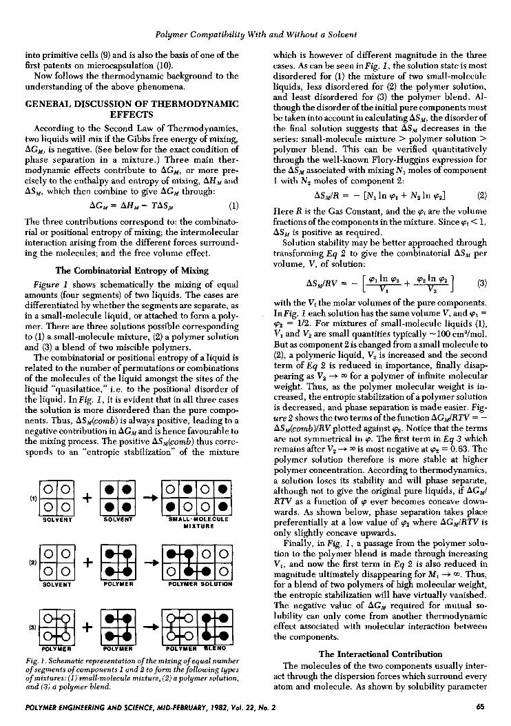
The Combinatorial Entropy of Mixing Figure 1 shows schematically the mixing of equal

amounts (four segments) of two liquids. The cases are differentiated by whether the segments are separate, as in a small-molecule liquid, or attached to form a polymer. There are three solutions possible corresponding to (1) a small-molecule mixture, (2) a polymer solution and (3) a blend of two miscible polymers.

The combinatorial or positional entropy of a liquid is related to the number of permutations or combinations of the molecules of the liquid amongst the sites of the liquid “quasilattice,” i. e. to the positional disorder of the liquid. In Fig. 1 , it is evident that in all three cases the solution is more disordered than the pure components. Thus, ASiM(cornb) is always positive, leading to a negative contribution in AGM and is hence favourable to the mixing process. The positive ASM(c0mb) thus corresponds to an “entropic stabilization” of the mixture

0 0 0 . SOLVENT SOLVENT SMALL- MOLECULE

MIXTURE

(2fq + Bl +ml 0 0 SOLVENT POLYMER POLYMER SOLUTION

(3)

POLY YER

Fig. 1 . Schematic representation of the mixing of equal number of segments of components 1 and 2 to form the following types of mixtures: (I).small-molecule mixture, (2 ) a polymer solution, and (3) a polymer blend.

which is however of different magnitude in the three cases. As can be seen inFig. 1, the solution state is most disordered for (1) the mixture of two small-molecule liquids, less disordered for (2) the polymer solution, and least disordered for (3) the polymer blend. Al- though the disorder of the initial pure components must be taken into account in calculating ASM, the disorder of the final solution suggests that AS,+, decreases in the series: small-molecule mixture > polymer solution > polymer blend. This can be verified quantitatively through the well-known Flory-Huggins expression for the ASM associated with mixing N1 moles of component 1 with N , moles of component 2:

ASM/R = - [ N , In cpl + N2 In cpz] (2) Here R is the Gas Constant, and the cpi are the volume fractions of the components in the mixture. Since qi < 1, A S M is positive as required.

Solution stability may be better approached through transforming Eq 2 to give the combinatorial AS,M per volume, V , of solution:

with the Vi the molar volumes of the pure components. In Fig. 1 each solution has the same volume V , and v1 = ‘ ~ 2 = 1/2. For mixtures of small-molecule liquids (l), Vl and Vz are small quantities typically -100 cm3/mol. But as component 2 is changed from a small molecule to (2), a polymeric liquid, Vz is increased and the second term of Eq 2 is reduced in importance, finally disappearing as Vz + CQ for a polymer of infinite molecular weight. Thus, as the polymer molecular weight is increased, the entropic stabilization of a polymer solution is decreased, and phase separation is made easier. Fig- ure 2 shows the two terms of the function AGMlRTV = - ASM(comb)/RV plotted against vz. Notice that the terms are not symmetrical in cp. The first term in Eq 3 which remains after V, --* CQ is most negative at pZ = 0.63. The polymer solution therefore is more stable at higher polymer concentration. According to thermodynamics, a solution loses its stability and will phase separate, although not to give the original pure liquids, if AGM/ RTV as a function of cp ever becomes concave down- wards. As shown below, phase separation takes place preferentially at a low value of cp2 where AG$RTV is only slightly concave upwards.

Finally, in Fig. 1 , a passage from the polymer solution to the polymer blend is made through increasing V , , and now the first term in Eq 2 is also reduced in magnitude ultimately disappearing for MI + CQ. Thus, for a blend of two polymers of high molecular weight, the entropic-stabilization will have virtually vanished. The negative value of AGM required for mutual solubility can only come from another thermodynamic effect associated with molecular interaction between the components.

The Interactional Contribution The molecules of the two components usually inter-

act through the dispersion forces which surround every atom and molecule. As shown by solubility parameter

POLYMER ENGINEERING AND SCIENCE, MID-FEBRUARY, 1982, YO/. 22, NO. 2 65

Donald Patterson

1

Fig. 2. The combinatorial entropy and the interactional contributions to the free energy of mixing, AGM, per unit volume and in units of RT against volume fraction, ipu of the second component (from E 9 3 or 6). The first and second terms of E 9 6 are calculated with V, = V2 = 100 cm3and shown as, respectively, curves a and b, with their total as cume c. When V2 + =, corresponding to a high polymer solution, only curve a remains. Curve d gives the interactional term with x12/V1 = 0.01 cm-3, above the critical value from E9 8. The sum of curves d and a gives the total curue e for the high polymer solution showing a concave-downward portion corresponding to solution instabil- ity at low v2. For a mixture of two high polymers only the interactional term remuins and no mixing takes place.

theory (ll), the dispersion force interaction or random dipole-induced dipole interaction (11) always leads to a positive contribution to AGM. It therefore cannot be the cause of polymer compatibility. However, a negative contribution to AGu arises in the much rarer case of “specific interactions.” These, as indicated below are usually associated with charge transfer or hydrogen- bonding between the components.

For either dispersion forces or specific interactions, the main effect is on the enthalpy of mixing AHu, positive and unfavourable to mixing for dispersion forces and negative and favourable in the case of specific interactions. More quantitatively, we have

AH,IRTV = (*) p1p2 = - XlZ v1 (P192 (4)

Here z is the lattice coordination number, k the Boltzmann Constant, Aw12 the energy change associated with creating a new contact of type (1-2) in the mixture between segments of types 1 and 2, and V, is the molar volume of a segment such as one of those in Fig. 1. Finally, xlZ is as defined by Flory (12), i.e. referred to a whole molecule of component 1 containing r1 segments.

Then, combining Eq 4 with Eq 3 for AS&omb), AGM

becomes

( 0 1 ~ 2 (6) XI2 +- Vl

+com bina t o r ial+ +interactional+

Note that x as defined inEq 5 is not the best measure of interaction between polymers 1 and 2 since it depends on the number of segments, r,, in component 1. Thus in a blend, where rl + m, xlZ + m. The important quantity is not x12 but ~ ~ ~ l r , or x12/Vl as in Eqs 4 and 6, and this quantity is independent of the molecular weight of polymer 1 and of the way in which a segment is defined.

The first two terms of Eq 6 have already been shown in Fig. 2. The third term with xI2 positive is concave- downward, and hence if of sufficient magnitude must cause phase separation (total AGM/RTV concave- downward) in the polymer solution at a small value of the polymer volume fraction, (p2. This is the well-known polymer solution phase separation, discussed for instance in Ref. 12. In the case of a blend of two high molecular-weight polymers, where V, and Vz + a, the combinatorial terms in Eq 6 are zero, and a positive value of xlZ leads to concave-downward behavior of AGuIRTV throughout the whole concentration range. Thus the mixture will separate into the pure polymers, and the condition given by Eq 6 for phase separation is just that xI2 and AGu be positive.

Figure 3 depicts schematically the temperature dependence of x12/VI, as suggested by the presence of T in the denominator of Eq 5. As T decreases, the positive,

8

Fig. 3. Schematic representation of contributions to xIp/VI: a, a’, the interactionul contribution for dispersion forces and specijic interactions resp.; b, the free volume contribution; c, the total xI2/VI in the case of dispersion forces, and d, the total x,2/V, for specific interactions. The critical value is shown for (I solution containing a polymer of infinite molecular weight.

66 POLYMER ENGINEERING AND SCIENCE, MID-FEBRUARY, 1982, Vol. 22, No. 2


unfavourable, dispersion force x12 becomes more posi- tiue, finally causing phase separation. On the other hand, the negative, favourable, specific interaction xlz becomes more negative, causing greater stability of, for instance, a blend.

The Free Volume Contribution The representation of the formation of a polymer

solution in Fig. 1 is not completely accurate and should be replaced by Fig. 4 , where one recognizes that the solvent liquid has large, and the polymer small, free volume. Figure 1 is also inaccurate in assuming that no volume change takes place during mixing whereas, as shown in Fig. 4 , the solution has free volume closer to the polymer than to the solvent. Thus, the effect of a difference in free volumes of the two components is to introduce a negative contribution (net contraction) in AVM. The free volume effect brings the molecules of the system closer together and hence causes negative contributions* in AHM and ASM. These contributions do not cancel in AGM but leave a positive term unfavorable to mixing. By convention, any term in AGM which is not combinatorial falls into the xI2 parameter, so that the xlz parameter contains not only the interactional term already discussed but also a positive free volume contribution as shown in Fig. 3. With increase of T, the free volume difference between polymer and solvent increases as does the corresponding contribution in xI2. For dispersion forces the sum of the two contributions gives a U-shaped curve bringing about phase separation at both low (UCST) and high (LCST) temperatures. On the other hand, the specific interactions case gives a sloping curve from negative to positive xlz allowing only the possiblity of an LCST.

The actual critical value of xlz is found through appli- cation in E q 6 of the critical conditions

If x is independent of cp,

Here again one finds the different degrees of entropic stabilization seen in Fig. 1 . If V, = V,, (x12/Vl)Crit = 2/V,, i.e. xI2 = 2, as found in the regular solution theory for small-molecule mixtures. With increase of V, to give a

* A contraction is usual but the free volume effect may give AV, > 0 if one has the unusual combination of a slightly expanded liquid of low cohesive energy density mixed with a highly expanded liquid which has at the same time a high cohesive energy density. An example would be a polymer such as polyisobutylene in benzene. In spite of the expansion of the system arising from the free volume effect, it is still predicted that free volume should have a negative effect on AHr and ASr. Intuition does not lead to the correct answer here.

SOLVENT POLYMER POLYMER SOLUTION

Fig. 4 . The formation of a polymer solution from solljent and polymer liquids of different free volume.

polymer solution, (xlz/ Vl)crit decreases, ultimately reaching 1/2Vl as Vz + 00. Then, as V, increases (x12/VJcrit tends to zero, corresponding to the complete elimination of the entropic stabilization of the solution.

CALCULATIONS USING THE

SOLUTIONS AND BLENDS The schematic curves of Fig. 3 may be made quantita-

tive through some related theoretical developments which we may call the Prigogine-Flory theory (13). The original Flory-Huggins theory (12) was essentially concerned with the combinatorial entropy but x was expected to decrease with increasing T by reason of E q 4 . The Prigogine-Flory theory concentrates on the x parameter introducing interactional and free volume effects giving a different temperature dependence. McMaster (4) and Olabisi (14) have applied an extended form of Flory’s theory to polymer mixtures. However, for many purposes a simplified approximate form (5) can be used which gives the following expression for x:

PRIGOGINE-FLORY THEORY FOR POLYMER

interaction free volume - 4

3 1 < V!’3 < -

The interaction and free volume terms appear in E 9 9 characterized by molecular parameters X,,/PT and 7’. X,,/Pf is positive or negative depending on whether the interaction is dominantly dispersion or specific. The starred parameters are calculated from the equation of state properties of the component liquids. Thus 7’ re- flects the difference in free volumes or degrees of ther- mal expansion of the components. It is large for a polymer-solvent system, but even in the case of two polymers a difference of free volume will occur if the polymer chains are of different flexibility. The V*, sometimes called a “hard-core volume,” corresponds to the liquid volume at 0 K. In E q 8 Vf and_V2 replace the molar volumes. The reduced volume, V1, is a measure of free volume so that as the temperature increases fr2m 0 K (accessible only in theory) to the critical point, V:‘’ increases from 1 to 4/3. As this occurs, the interaction term decreases and the free volume increases in the appropriate manner.

Figure 5 shows a prediction made (5) using E q 9 for a typical pol ymer-solvent system corresponding approx- imately to polystyrene-cyclohexane. Both the UCST and LCST for infinite polymer molecular weight are found at accessible temperatures. Calculations (5) are then shown in Fig. 6 for an immiscible pair of polymers, one of which is polystyrene and again with X12 = 10 J/cm3. Various values Of T2 correspond to various differences in flexibilities of the chains and hence differences in free volume. The figure shows critical values of

POLYMER ENGINEERING AND SCIENCE, MID-FEBRUARY, 1982, Vol. 22, No. 2 67

Donald Patterson

-lo

1c

I I -

I I I I I

> 'E x n 52 -

I 1.05 1.10 1.15 1.20 1.25 C,l/n I I I I I I I

-273 -67 69 156 209 239 t"c Fig. 5. Polymer-solvent system. The Xlzparameter expressed per unit volume of interacting molecules, i.e. xI2 divided by Vf = M,of for a polymer(2)-solvent (1) system against V:I3and t. The following parameters have been used in E 9 9: T f = 5000 K , P f = 400 J cm-9 and T f = 8191 (polystyrene); XI, = 10 Jlcm3, a typical value for dispersion forces. The dashed curves give the interactional and free volume contributions, and the horizontal line corresponds to the critical value of x lJVf from E 9 8, put- ting Vf = 70 cm3 mol-'and letting M2 + op (after Ref. 5).

pLF?!I ___- I ---- ---- I ---- I - - -

9" 100 W 110 L15 l.20 l.25

I I I I I I -273 64 283 429 517 566

TEMPERATURE ("c) Fig. 6. Polymer-polymer system with xI2 > 0. The xlz/Mlv:' parameter for a mixture of polymers intgracting with dispersion forces with XI, = 10 J against V:I3 and t, with difierent values of T. Polystyrene is the reference polymer, T: = 8191 K , P f = 500 J and the horizontal lines are critical ualues of XI2/M,of from E9 8 with MI = M2 and uf = of = 1 g em-! (after Ref. 5).

xlJVp calculated from E q 8 for different values of the molecular weights which are assumed equal for the two

polymers and with the specific volume u* = V*/M = 1 cm3/g. Miscibility of the polymers occurs only when their molecular weights are very small, about one or two thousand. Although an LCST can be predicted, it lies at too high a temperature to be observed. With increase of molecular weight, the UCST rapidly increases so that for M greater than a thousand the system is phase sepa- rated at normal temperatures. This behavior is in fact observed experimentally in such systems (15).

Figure 7 shows the calculation (5) for the case of a miscible pair withx12 given a small negative value, - 1.3 J/cm3, which corresponds roughly to the polystyrene- poly(viny1 methyl ether) system. If the molecular weights are very high, ( ~ ~ ~ / V f ) ~ ~ i ~ =r 0 and an LCST is predicted at -160°C. As the molecular weights are lowered (x12/V1*)crit is increased, indicating increasing entropic stabilization, and the LCST rises, as can be seen in the experimental results of Nishi and Kwei (16) in Fig. 8.

McMaster (4) was the first to emphasize that the normal phase separation occurring in a blend is the LCST, and he has applied the Prigogine-Flory ideas in the Flory model (13b) to blends in a very complete manner (also see pp. 81-104 of Ref. 1). The approximate treat- ment of Ref 5 is also adequate to predict various fea- tures of polymer-polymer miscibility including the pressure dependence of the LCST. Nevertheless, polymer miscibility as such is not predicted by these theories, or by any other so far as the author is aware. To predict miscibility would require a theory of the specific interactions, leading to a prediction of negative x12 and

68 POLYMER ENGINEERING A N D SCIENCE, MID-FEBRUARY, 1982, Vol. 22, NO. 2

Polymer Compatibility With and Without a Soloent

250 I

I I I I 1 4 Qz a4 46 QB P

06 Fig. 8. Cloud point curves for PVEE and monodisperse PS mixture where molecular weight (M,,.) of PS is changed: 0, 10000; 0,20400; A, 51 000; 0,200000; 4 is the weight fraction of P S . {after Re$ 16).

negative A H M for the polymer pair of interest. All that can be done is to suggest the kind of specific interaction between the polymers in a pair known to be miscible, and even here the answer may not be clear. Thus poly(viny1 chloride) is miscible with many other polymers or plasticizers which contain an ester or ether oxygen. This has usually been attributed (1, 17) to a weak hydrogen-bond between the oxygen and an a-hydrogen on the chlorine-bearing carbon of the PVC. This is by analogy with the much-studied H-bond between the oxygen in small-molecule esters, ethers and ketones and the hydrogen in chloroform which results in negative values of AHlw when these components are mixed (18). Again AHM is very strongly negative (19) when the oxygen-containing molecule interacts with a chlorinated hydrocarbon where the hydrogen is attached to a carbon bearing two chlorines. However, the situation is different for PVC and here Pouch19 and Biro3 (20) have given evidence that the polymer miscibility involves the oxygen and the chlorine atoms of the PVC. Thus, a number of chlorinated hydrocarbon small-molecules give (20) similar negative A H M values when mixed with the ether tetrahydrofuran, and this is independent of whether there is a hydrogen in the a-position or not. Furthermore, CC14 + THF also gives (20) a large negative AHIM.Indeed it is well known that CC14 mixes with many ethers and esters with large negative A H M (18), the sign apparently being due to a weak charge-transfer (CT) interaction where the oxygen is the electron donor and the C1 the acceptor.

It seems probable that charge transfer plays a consid- erable, and not always appreciated, role in polymer miscibility. For instance, Cruzet al. (21) have discussed polyester-polycarbonate miscibility in those terms, using the negative sign of A H M of small-molecule models of the polymers as a test for miscibility. In the

same way, the best-known miscible pair, polystyrene- poly(pheny1ene oxide) or Noryl, presumably also owes its miscibility to an electron donor-acceptor interaction.

I t is tempting to suggest that any pair of groups which interact in a small-molecule mixture to give a negative AHM should bring about miscibility when it occurs in a pair of polymers. However, the very specific interaction which gives the negative AHw also requires a special geometry of the contact, i.e. an ordering of the molecules in space, and hence gives a negative contribution in ASM which is unfavorable to mixing. The net effect in the final AGM will certainly be less negative then expected, and perhaps not be sufficient to achieve miscibility of the polymers.

CALCULATIONS INVOLVING TWO POLYMERS + SOLVENT

Completely new compatibility phenomena arise (6) for a ternary system containing a solvent (component 1) and two polymers (components 2 and 3). Using the Flory-Huggins theory, phase diagrams can be calculated (6) in terms of the x parameters for the interaction between the three pairs of components. Thus, here we are not concerned with predicting the temperature dependence of the x parameter, but rather finding the effect on the phase diagram of assumed or experimentally determined values of X. Figure 9 shows spinodals from Ref. 6. A spinodal separates an unstable region from the rest of the phase diagram. Although the binodal, separating the metastable from the stable regions is preferable, the spinodal is often used to obtain approximate information about the phase diagram. Binodals have been used inRef. 7 with results similar to those given here from spinodals. In Fig. 9 the numbers of segments are rl = 1, r, = r, = 1000, so that the polymer molecular weights are high, -lo5. First, one

1

Fig. 9. Calculated spinodals for a ternary system; soloent ( l ) , polymer(2), and polymer(3). Values o f r l = 1 and r, = r, = I000 are taken for all curues. For spinodals a, b, and c . xZ3 = 0.0025, and the pairs of interaction parameters x l e x,3are as follows: (a) 0.40,0.40; (b)0.40,0.50;(b')0.40,0.30. Forspinodalscandc', xZ3 = 0.0 and xle x I 3 are the same as for (b) and (b'). Solution compositions are in volume fractions.

POLYMER ENGINEERING AND SCIENCE, MID-FEBRUARY, 1982, Vol. 22, NO. 2 69

considers the polymers to be slightly incompatible, ~ 2 3

per segment being 0.0025. To compare with Figs. 5-7 taking the molar volume of a segment to be -lo2 cm3/ mol, we have x23/V, = 2.5 x cm-3 which is about fifty times less than x12/Vf values shown in Fig. 6. Due to this small degree of incompatibility, a moderately large region of phase separation occurs in the 2-3 binary along the bottom edge of the triangle in Fig. 9. Next, a solvent is added for which the polymers have equal affinity, x 1 2 = ~ 1 3 = 0.40 per segment, or expressed per volume, x12/Vf = 4 x which is similar to the values in Fig. 5 . With increase of solvent concentration the two-phase region becomes narrower and finally at about 20 percent solvent by volume the three components are completely miscible. It is of interest for what follows that the region of phase separation is independent of the value of x12 and ~ 2 3 provided that they are equal (and are less than the critical value of phase separation along the 1-2 and 1-3 binaries). Shown next in Fig. 9 is the spinodal calculated with the same value of ~ 2 3 and of x12, but increasing the ~ 1 3 , to 0.5, i.e. making the 1-3 interaction worse (full curve b). The region of incompatibility has now increased dramatically. But, if x i 3 is decreased from 0.4 to 0.3 making the 1-3 interaction better, one has almost the same phase diagram as before (curve b’). Thus the growth in the region of incompatibility is independent of whether the 1-3 interaction has been made worse or better. What counts is the magnitude of the difference between the two polymer- solvent x parameters, i.e. [AX[. Next, the ~ 2 3 interaction may be decreased to zero so that the two polymers be- come compatible. In this case, if [Ax[ = 0, there is no phase separation at all, but keeping xI2 = 0.4 and using x13 = 0.5 or 0.3 leads to the closed regions c and c‘ where phase separation still occurs inside the triangle. This type of phase separation produces two coexisting solutions having the same concentration of total polymer, but one is rich in polymer 2 and the other in polymer 3. The closed loops due to the [Ax[ effect have been found now in many systems including polystyrene-poly(viny1 methyl ether) (22) in chloroform, trichloroethylene and dichloromethane, and several compatible polymer pairs containing poly(viny1 chloride) mixed with chlorinated hydrocarbon solvents (23).

The polystyrene-poly(viny1 methyl ether)/ trichloroethylene case has been studied in detail (22b). The x parameters for the two polymer-solvent interactions were obtained using the gas-liquid chromatography method (inverse chromatography), and they are shown as functions of temperature in Fig. 10. The x parameter for the PS-trichloroethylene interaction has usual dispersion force values and, with change of temperature, it roughly follows the theoretical U-shape. However, the PVME-trichloroethylene interaction is much more attractive due to a specific interaction, involving the ether oxygen in either a hydrogen bond or a charge transfer interaction with the chlorine (or perhaps both). The x parameter is negative at low T, but becomes less negative with increase of T. Thus, /AX[ for this system de‘creases rapidly with T, passes through a

TEMPERATURE (”c) 0

Donuld Patterson

70 POLYMER ENGINEERING AND SCIENCE, MID-FEBRUARY. 1982, Vol. 22, No. 2

-02V -03

-0AL Fig. 10. The temperature dependence of xfor the interaction of trichloroethene w i t h polystyrene (x,a and w i th poly(uiny1 methyl ether)(x,J as determined by the GLC method. (afterRef. 22b).

minimum and then, according to Fig. 10, it increases again at high T. The region of phase separation should therefore occur at low T (a UCST) then, with increase of T, it should contract and disappear, only to reappear and expand at higher T (an LCST). A view of the predicted and observed behavior is seen in Fig. 11 for PVME of 10,000 molecular weight and a range of molecular weights for polystyrene. With a molecular weight of 2100 for PS, phase separation is found only at a UCST at low T, and presumably occurs again at an LCST which is too high to be observed. With larger molecular weights for PS, entropic stabilization is reduced so that the UCST increases and the LCST decreases. Finally, the UCST and LCST coalesce to form an “hour-glass’’ phase diagram in which there is no temperature with complete miscibility of the components. The phase diagrams calculated from the Flory- Huggins theory agree very satisfactorily with the experimental data.

TWO HIGHLY COMPATIBLE POLYMERS + SOLVENT

Phase separation can still occur in a ternary mixture containing two compatible polymers and a solvent even if xlz = x13. Figure 12 illustrates this phenomenon which arises when the attraction between the polymers becomes extremely large (24). The number of segments in the solvent molecule is 1, and each polymer is small here, r = 9, and xI2 = xI3 = 0.6, i.e. less than the critical value for phase separation in a binary. The parameter varied is ~ 2 3 which passes from a positive to a large negative value. As ~ 2 3 per segment falls from 1.0 to 0.5, the spinodals decrease in size as expected, and when x12 = 0, no phase separation occurs at all. This situation continues until ~ 2 3 reaches a value of -2.0 when a closed solubility loop appears having roughly the same

Polymer Compatibility With and Without u Solvent

Q5 1.0 0 a5 10

TOTAL POCYMER WEIGHT FRACTION TOTAL POCYMER WEIGHT FRACTION

(a) (b) Fig. 11 a. Cloud point temperatures formixturesof equal weights of PVME and PS of indicated molecular weights with trichloroethene, as a function of the weight fraction of total polymer in the mixture. Molecular weight of PVME = lo4. (b) Simulation of Fig. l i (a ) using theoretical spinoduls calculated with xlz and xI3 values f m m Fig. 10 and fis from experiment is essentially zero. The number of segments are as follows: 7 3 = rPV.HE = 148; r2 ,ps (2100) = 221; r2,ps(37000) = 382; r 2 . p s ( 5 0 ~ o ) = 51 7; ~ Z , P S ~ ~ ~ O W O ) = 1137. (after Ref. 22b).

shape as the loops previously encountered in Fig. 9. The loop expands as ~ 2 3 becomes more negative, e.g. to -3.0. Although the loop is similar in shape to that found in the [Ax1 effect, the phase separation phenomenon is different in character. Vertical “tie-lines’’ are found indicating that the two coexisting phases are, respectively, dilute and concentrated in polymer just as they are in a polymer solution. The 2-3 composition of the total polymer in each phase will be the same. Thus here the two polymers are not separating away from each other as in the [Ax1 effect, but rather there is a separation of the polymers together away from the solvent. The two polymers have such a high affinity for one another that they do not mix well with the solvent.

A changeover from positive to negative ~ 2 3 behavior is found in the gelatidgum arabiclwater system as shown in Fig. 1 3 taken from Ref 8. At a pH below the isoelectric point of gelatin the two polymers are similarly charged. Thus there is a repulsive interaction, i.e. ~ 2 3 is positive. The phase diagram shown in Fig. 13a has the shape predicted for positive ~ 2 3 and the tie-lines are horizontal. At a pH higher than the isoelectric point of gelatin, the two polymers are oppositely charged, and corresponding to the net attraction there is a negative value of ~ 2 3 . Hence the phase diagram in Fig. 13b has the shape predicted in Fig. 12 for negative x23 and the

POLYMER ENGINEERING AND SCIENCE, MID-FEBRUARY, 1982, Vol. 22, NO. 2

tie-lines are vertical. In the older terminology (8) the two types of phase separation are called simple and complex coacervation. The gelatidgum arabidwater system and complex coacervation are the basis of a micro-encapsulation technique (10) to form “carbon-

Fig. 12 Spinodals fora ternary system containing two polymers (components 2 and 3) and a solvent (component I) for different x 2 3 ualues. For all curves x , ~ = x13 = 0.6; rI = 1; r2 = r, = 9. The values of xZ3 are as indicated. When xZ3 = 0, miscibility is observed for the whole concentration range. Circles show the position of the calculated critical points. They indicate the tie-lines are horizontal for xZ3 > 0, and vertical for ~ 2 3 < 0.

71

Donald Patterson

/ \ \ \ \ \

G50’ 20 40 60 80 A

Fig. 13. Cloud-point curves for the gelatin(G)lgum arabic (A)l water(W) system. (a) Cloud-point curve obtained at a p H below the isoelectric point of gelatin. Tie-lines connect liquids which are rich in G and relatively poor in A (on the left-hand branch) with liquids which are rich in A and relatively poor in G (on the right-hand branch). (b) Cloud-point curve obtained at a p H above the isoelectric point of gelatin. The coacervates which are rich both in G and in A are to be found on the arched branch of the curve in plane of the triangle. The equilibrium liquids which are poor both in G and in A lie on a branch of the curve close to the water-corner of the triangle. (after Re$ 8).

less” paper. Bringing the system into the two-phase region in Fig. 13b separates the solution into almost pure water and a concentrated gelatin-gum arabic mixture which precipitates on the surface of dispersed ink globules encapsulating them.

Although most systems showing complex coacervation have been aqueous, Morawetz et al. (25) have demonstrated that this behavior can be found with un- charged polymers in a non-aqueous solvent. The work starts with polystyrene and poly(methy1 methacrylate) which are incompatible and give simple coacervation in several solvents. The phase diagrams are similar to that already seen in Fig. 13a. However, methacrylic acid segments may be built into the PMMA chain and basic 4-vinylpyridine segments into the polystyrene chain so that the overall repulsion between the polymers is re-

duced. Thus compatibility is brought about and the ternary phase diagram shows no phase separation. With increase in the number of co-monomers net attraction increases, and finally, presumably at a large negative value of x23, the phase separation again appears in the ternary diagram, this time corresponding to Fig. 13b.

It has been stressed in the above that polymer systems present a rich variety of phase separation phenomena which are only now beginning to be explored. Fur- thermore, they are amenable, at least in a semi- quantitative way to simple treatments based on the Flory-Huggins theory. Where the temperature dependence of the x parameters is required, an approximate form of the Prigogine-Flory theory is successful.

ACKNOWLEDGMENT I wish to thank the Natural Sciences and Engineering

Research Council of Canada and the Ministkre de 1’Education du Quhbec for their support of much of the research forming the basis of this review.

Appreciation is expressed to the Editors of Mac- romolecules for permission to use Figs. 5-7 and 9-12, and to the Editors ofPolymer for Fig. 8 and Elsevier for Fig. 13.

DISCUSSION R. E. PRUD’HOMME Is it correct to state that the Flory-Prigogine theory does not lead to the prediction of an Upper Critical Solution Temperature for compatible polymer-polymer mixtures? Recent results presented by Wendoff on PVF2- PMMA blends Q. Polym. Sci., Polym. Lett. Ed., 18,439 (1980)) and by Stein (unpublished yet) indicate that the thermodynamic interaction parameter x varies greatly with composition in polymer-polymer blends. Is it expected behavior and could it be considered as a general situation? I would like to point out that in general the so-called compatible polymer-polymer blends present a T,- composition curve which is concave. Very strong interactions between the two polymers are necessary to pro- duce a straight line or a convex T,-composition curve. This latter behavior was recently obtained by Kwei et al. Q. Polym. Sci., Polym. Lett. Ed., 18, 201 (1980)). In one instance, for a PVN02-PVA, blend, a maximum was even reported (Akiyama S., Bull. Chem. SOC. Ja- pan, 45, 1381 (1972)).

D. D. PATTERSON Given a negative value of the XI2 parameter, which would be required for the compatibility of two high molecular weight polymers, then indeed only an LCST would be predicted. The occurrence of a UCST could be taken account of in the formalism by introducing the Q12 parameter with a positive value, but this could not be predicted in a natural way. In general, if there is a difference in surface/volume ratio of the two components the theory predicts that x should vary with the concentration. However, this dif-

72 POLYMER ENGINEERING AND SCIENCE, MID-FEBRUARY, 1982, V O ~ . 22, NO. 2


ference has to be verv laree in order to obtain the sort of 10. B. K. Green and L. Schleicher, U.S. Patent 2800457 as- 2 -

variations of x which can be found experimentally. It is perhaps more likely that in polymer blends the varia- . tion of x arises from the molecules having different interaction sites on their surfaces, e . g. sites capable of entering into specific interactions and others which interact through ordinary dispersion forces. Such situa- tions can certainly give rise to a strong variation of the x parameter with the concentration. For their description something more complex than the simple Flory- Huggins theory would be required, e. g. quasi-chemical approach.

REFERENCES 1. For a detailed and authoritative discussion see 0. Olabisi,

L. M. Robeson and M. T. Shaw, “Polymer-Polymer Misci- bility,” Academic Press, New York (1979).

2. D. Patterson, Macromolecules, 2,674 (1969). 3. P. J. Freeman and J. S. Rowlinson, Polymer, 1, 20 (1960). 4. L. P. McMaster, Macromolecules, 6, 760 (1973). 5. D. Patterson and A. Robard, Macromolecules, 11, 690

6. L. Zeman and D. Patterson, Macromolecules, 5,513 (1972). 7. C. C. Hsu and J. M. Prausnitz, Macromolecules, 7, 320

8. H. G. Bungenberg de Jong in “Colloid Science,” H. R.

9. A. I. Oparin, “Life, its Nature, Origin and Development,”

(1978).

(1974).

Kruyt, Ed., pp. 355-364, Elsevier, New York (1952).

pp. 39-80, Academic Press, New York (1961).

signed to National Cash Register Co., July 23, 1957. 11. R. L. Scott and. J. L. Hildebrand, “The Solubility of Non-

Electrolytes,” Reinhold, New York (1951). 12. P. J. Flory, “The Principles of Polymer Chemistry,” Ch. 12,

Cornell University Press (1953). 13. (a) I. Prigogine (with the collaboration of V. Mathot and A.

Bellemans), “The Molecular Theory of Solutions,” Chs. 16 and 17, North-Holland, Amsterdam (1967).(b) P. J. Flory, Disc. Faraday SOC., 49, 7 (1970).

14. 0. Olabisi, Macromolecules, 8, 316 (1975). 15. R. Koninsgveld, L. A. Kleintjens, and H. M. Scheffeleers,

Pure Appl. Chem., 39, 1 (1974); R. Koningsveld and L. A. Kleintjens, Brit. Polym. J . , 9, 212 (1977).

16. T. Nishi and T. K. Kwei, Polymer, 16, 285 (1975). 17. R. L. Adelman and I. M. Klein,]. Polym. Sci., 31,77 (1958). 18. See for instance, L. A. Beath and A. G. Williamson,J. Chem.

Thermodynamics, 1,51 (1969). 19. C. S. Marvel, M. J. Copley, and E. Ginsberg, J . Am. Chem.

SOC., 62, 3109 (1940). 20. J . Pouchlf and J. Biro3,J. Polym. Sci., Pt. B , 7,463 (1969); J.

Pouchlf, A , “ Zivnf and J. Biro3, J . Chim. Phys., 72, 385 (1975).

21. C. A. Cruz, J. W. Barlow, and D. R. Paul, Macromolecules, 12, 726 (1979).

22. (a) A . Robard, D. Patterson, and G. Delmas, Mac- romolecules, 10, 706 (1977). (1)) A. Robard and D. Patterson, ibid., 10, 1020 (1977).

23. W. P. Kwang, M.Sc. thesis, McGill University, 1980. 24. A. Robard, Ph.D. thesis, McGill University, 1978, Ch. 3. 25. H. Morawetz, R. N . Goldberg, and S. Djadoun, Mac-

romolecules, 10, 1015 (1977).

POLYMER ENGINEERING AND SCIENCE, MID-FEBRUARY, 1982, Vol. 22, NO. 2 73

polymer compatibility with and without a solvent

Documents