polymorphic type inference for languages with overloading

POLYMORPHIC TYPE INFERENCE

FOR LANGUAGES WITH OVERLOADING AND

SUBTYPING

A Dissertation

Presented to the Faculty of the Graduate School

of Cornell University

in Partial Fulfillment of the Requirements for the Degree of

Doctor of Philosophy

by

Geoffrey Seward Smith

August 1991

POLYMORPHIC TYPE INFERENCE

FOR LANGUAGES WITH OVERLOADING AND SUBTYPING

Geoffrey Seward Smith, Ph.D.

Cornell University 1991

Many computer programs have the property that they work correctly on a variety

of types of input; such programs are called polymorphic. Polymorphic type systems

support polymorphism by allowing programs to be given multiple types. In this

way, programs are permitted greater flexibility of use, while still receiving the

benefits of strong typing.

One especially successful polymorphic type system is the system of Hindley,

Milner, and Damas, which is used in the programming language ML. This type

system allows programs to be given universally quantified types as a means of

expressing polymorphism. It has two especially nice properties. First, every well-

typed program has a “best” type, called the principal type, that captures all the

possible types of the program. Second, principal types can be inferred, allowing

programs to be written without type declarations. However, two useful kinds of

polymorphism cannot be expressed in this type system: overloading and subtyping.

Overloading is the kind of polymorphism exhibited by a function like addition,

whose types cannot be captured by a single universally quantified type formula.

Subtyping is the property that one type is contained in another, as, for example,

int ⊆ real .

This dissertation extends the Hindley/Milner/Damas type system to incorpo-

rate overloading and subtyping. The key device needed is constrained universal

quantification, in which quantified variables are allowed only those instantiations

that satisfy a set of constraints. We present an inference algorithm and prove that

it is sound and complete; hence it infers principal types.

An issue that arises with constrained quantification is the satisfiability of con-

straint sets. We prove that it is undecidable whether a given constraint set is

satisfiable; this difficulty leads us to impose restrictions on overloading.

An interesting feature of type inference with subtyping is the necessity of sim-

plifying the inferred types—the unsimplified types are unintelligible. The sim-

plification process involves shape unification, graph algorithms such a strongly

connected components and transistive reduction, and simplifications based on the

monotonicities of type formulas.

Biographical Sketch

Geoffrey Seward Smith was born on December 30, 1960 in Carmel, California. His

childhood was spent in Bethesda, Maryland. In 1982, he graduated, summa cum

laude, fram Brandeis University with the degree of Bachelor of Arts in Mathe-

matics and Computer Science. In 1986, he received a Master of Science degree

in Computer Science from Cornell University. He was married to Maria Elena

Gonzalez in 1982, and in 1988 he and his wife were blessed with a son, Daniel.

iii

To Elena and Daniel

iv

Acknowledgements

My advisor, David Gries, has been a patient, encouraging teacher. His high stan-

dards and devotion to the field have been an inspiration to me. His warmth and

humanity have made it a pleasure to work with him.

Thanks also to my other committee members, Dexter Kozen and Stephen

Chase. I have always marveled at Dexter’s depth and breadth of knowledge; he

has taught me a great deal throughout my years at Cornell.

Cornell has been a wonderful place to learn and grow; I am indebted to many

people here who have taught and inspired me. Dennis Volpano discussed much

of the material in this dissertation with me, and his comments and suggestions

helped to shape this work. Bard Bloom gave me valuable insight into the shape

unification problem. Discussions with Hal Perkins, Earlin Lutz, Steve Jackson,

Naixao Zhang, and the other members of the Polya project have added greatly to

my understanding of programming languages and type systems.

I have had a very nice group of officemates during my time at Cornell. For

friendship, advice, and encouragement, I thank Amy Briggs, Jim Kadin, Daniela

Rus, and Judith Underwood.

Finally, I thank Elena and Daniel for their love and support across the years.

v

Table of Contents

1 Introduction 11.1 Types . . . . . . . . . . . . . . . . . . . . . . . . . . . . . . . . . . 11.2 Reductionist Type Correctness . . . . . . . . . . . . . . . . . . . . . 21.3 Polymorphism . . . . . . . . . . . . . . . . . . . . . . . . . . . . . . 41.4 Axiomatic Type Correctness . . . . . . . . . . . . . . . . . . . . . . 81.5 The Hindley/Milner/Damas Type System . . . . . . . . . . . . . . 121.6 Extensions to Hindley/Milner/Damas Polymorphism . . . . . . . . 15

2 Overloading 192.1 The Type System . . . . . . . . . . . . . . . . . . . . . . . . . . . . 20

2.1.1 Types and Type Schemes . . . . . . . . . . . . . . . . . . . 202.1.2 Substitution and α -equivalence . . . . . . . . . . . . . . . . 212.1.3 The Typing Rules . . . . . . . . . . . . . . . . . . . . . . . . 252.1.4 The Instance Relation and Principal Types . . . . . . . . . . 31

2.2 Properties of the Type System . . . . . . . . . . . . . . . . . . . . . 342.3 Algorithm Wo . . . . . . . . . . . . . . . . . . . . . . . . . . . . . 432.4 Properties of Wo . . . . . . . . . . . . . . . . . . . . . . . . . . . . 49

2.4.1 Soundness of Wo . . . . . . . . . . . . . . . . . . . . . . . . 492.4.2 Completeness of Wo . . . . . . . . . . . . . . . . . . . . . . 53

2.5 Limitative Results . . . . . . . . . . . . . . . . . . . . . . . . . . . 742.5.1 A Logical Digression . . . . . . . . . . . . . . . . . . . . . . 80

2.6 Restricted Forms of Overloading . . . . . . . . . . . . . . . . . . . . 812.7 Conclusion . . . . . . . . . . . . . . . . . . . . . . . . . . . . . . . . 84

3 Subtyping 853.1 The Type System . . . . . . . . . . . . . . . . . . . . . . . . . . . . 85

3.1.1 Types and Type Schemes . . . . . . . . . . . . . . . . . . . 863.1.2 Substitution and α -equivalence . . . . . . . . . . . . . . . . 863.1.3 The Typing Rules . . . . . . . . . . . . . . . . . . . . . . . . 873.1.4 The Instance Relation . . . . . . . . . . . . . . . . . . . . . 89

3.2 Properties of the Type System . . . . . . . . . . . . . . . . . . . . . 893.3 Algorithm Wos . . . . . . . . . . . . . . . . . . . . . . . . . . . . . 963.4 Properties of Wos . . . . . . . . . . . . . . . . . . . . . . . . . . . . 97

vi

3.4.1 Soundness of Wos . . . . . . . . . . . . . . . . . . . . . . . 973.4.2 Completeness of Wos . . . . . . . . . . . . . . . . . . . . . . 98

3.5 An Example Assumption Set . . . . . . . . . . . . . . . . . . . . . . 1173.6 Type Simplification . . . . . . . . . . . . . . . . . . . . . . . . . . . 120

3.6.1 An Overview of Type Simplification . . . . . . . . . . . . . . 1203.6.2 Transformation to Atomic Inclusions . . . . . . . . . . . . . 1263.6.3 Collapsing Strongly Connected Components . . . . . . . . . 1313.6.4 Monotonicity-based Instantiations . . . . . . . . . . . . . . . 1333.6.5 Function close . . . . . . . . . . . . . . . . . . . . . . . . . . 140

3.7 Satisfiability Checking . . . . . . . . . . . . . . . . . . . . . . . . . 1403.8 Conclusion . . . . . . . . . . . . . . . . . . . . . . . . . . . . . . . . 146

4 Conclusion 1484.1 A Practical Look at Type Inference . . . . . . . . . . . . . . . . . . 1484.2 Related Work . . . . . . . . . . . . . . . . . . . . . . . . . . . . . . 1524.3 Future Directions . . . . . . . . . . . . . . . . . . . . . . . . . . . . 154

4.3.1 Satisfiability of Constraint Sets . . . . . . . . . . . . . . . . 1544.3.2 Records . . . . . . . . . . . . . . . . . . . . . . . . . . . . . 1544.3.3 Semantic Issues . . . . . . . . . . . . . . . . . . . . . . . . . 1544.3.4 Imperative Languages . . . . . . . . . . . . . . . . . . . . . 155

A Omitted Proofs 156

Bibliography 157

vii

List of Figures

2.1 Typing Rules with Overloading . . . . . . . . . . . . . . . . . . . . 262.2 Algorithm Wo . . . . . . . . . . . . . . . . . . . . . . . . . . . . . 442.3 Function close . . . . . . . . . . . . . . . . . . . . . . . . . . . . . 462.4 Example lexicographic . . . . . . . . . . . . . . . . . . . . . . . . . 48

3.1 Additional Rules for Subtyping . . . . . . . . . . . . . . . . . . . . 873.2 Algorithm Wos . . . . . . . . . . . . . . . . . . . . . . . . . . . . . 963.3 Assumption Set A0 . . . . . . . . . . . . . . . . . . . . . . . . . . 1183.4 Atomic Inclusions for lexicographic . . . . . . . . . . . . . . . . . . 1233.5 Collapsed Components of lexicographic . . . . . . . . . . . . . . . . 1243.6 Result of Shrinking ι , υ , λ , ζ , φ , µ , and θ . . . . . . . . . . . 1253.7 Function shape-unifier . . . . . . . . . . . . . . . . . . . . . . . . . 1283.8 Function atomic-inclusions . . . . . . . . . . . . . . . . . . . . . . 1293.9 Function component-collapser . . . . . . . . . . . . . . . . . . . . . 1323.10 Function close . . . . . . . . . . . . . . . . . . . . . . . . . . . . . 141

4.1 Example fast-expon . . . . . . . . . . . . . . . . . . . . . . . . . . 1494.2 Example mergesort . . . . . . . . . . . . . . . . . . . . . . . . . . . 1514.3 Example reduce-right . . . . . . . . . . . . . . . . . . . . . . . . . . 1524.4 Example another-reduce-right . . . . . . . . . . . . . . . . . . . . . 152

viii

Chapter 1

Introduction

Over the years, the notion of types in programming languages has grown steadily in

importance and depth. In recent years, the study of types has been enriched by the

introduction of ideas from mathematical logic. Yet, many basic questions about

types remain unresolved—there is still no consensus about what exactly types are,

or about what it means for a computer program to be type correct. What follows

in this chapter, then, is an attempt to outline what is most important about types

and type systems.

1.1 Types

It seems fundamental to human intelligence to classify the objects of the world

based on their observed similarities and differences. This process of classification

is a basic way of dealing with the complexity of the world: by grouping together

similar objects, we may abstract away from particular objects and study properties

of the group as a whole.

In the realm of mathematics, the process of grouping together similar objects

1

has led to the identification of a rich diversity of mathematical structures, for

example Euclidean spaces, topological spaces, and categories. The study of a

mathematical structure leads to the development of a theory of the structure;

the theory describes the common properties of the members of the structure and

facilitates reasoning about the structure. Reasoning about a structure is further

facilitated by the establishment of specialized notation tailored to the structure.

Many mathematical structures are also useful computational structures; for

example graphs, sets, and sequences are especially useful in programming. In

computer science, we call such structures types.

A type, then, is a set of elements and operations having an associated theory

that allows reasoning about manipulations of elements of the type.

The programming process is much easier in a language with a rich collection of

types; this is perhaps the most important feature of high-level languages. Hence

a major consideration in the design of any such language is how types will be

supported. Type support may be divided into two relatively independent aspects:

first, to ensure that high-level types are correctly implemented in terms of the

low-level data structures available on an actual machine, and second, to ensure

that programs use types only in ways that are sensible. The first of these we call

reductionist type correctness, the second we call axiomatic type correctness. We

explore these in more detail in the next three sections.

1.2 Reductionist Type Correctness

Since actual machines have but a few types (for example, integers of various sizes,

floating-point numbers, arrays, and pointers), a major task of a compiler is to

implement the types of a high-level language in terms of low-level data structures.

The implementation of types is complicated by the fact that many types (for ex-

2

ample, sets) have no best implementation that is appropriate for all situations.

Instead, different implementations should be used depending on the kind and fre-

quency of the operations to be performed.

As a rule, programming languages have not attempted to use multiple imple-

mentations for built-in types1; instead, the usual approach is to provide a language

facility that allows the programmer to define a new type and to give its represen-

tation in terms of other types. The key issue is how to protect the representation

from misuse.

Suppose that we wish to implement a type dictionary with operations insert

and member? . We might choose to represent the dictionary as a bit-vector. But

this should not mean that type dictionary is the same as type bit-vector ! For,

outside the procedures insert and member? , there should be no access to the

underlying representation. Furthermore, just because a value has type bit-vector

we cannot conclude that the value represents a dictionary. The two concerns are

called “secrecy” and “authentication” by Morris [Mor73], and they lead him to

declare that “types are not sets”. This appears to contradict our definition of type

above, but this is really not the case. Morris is discussing what is needed for one

type to represent another; he is not discussing the nature of types.

In general, it can be argued that a failure to distinguish between reductionist

and axiomatic type correctness has led to a great deal of confusion about the nature

of types.

Cardelli and Wegner follow in the reductionist style when they state,

A type may be viewed as a set of clothes (or a suit of armor) that

protects an underlying untyped representation from arbitrary or unin-

tended use. [CW85, p. 474]

1SETL is an exception.

3

Similarly, in the language Russell [DD85], the notion of strong typing is defined so

that the meaning of a well-typed program is independent of the representations of

the types it uses. In a similar way, Mitchell and Plotkin [MP88] suggest that an

abstract type that is represented by another type should be given an existentially

quantified type as a way of hiding the representation.

Aho, Hopcroft, and Ullman [AHU83] assert that two types should be regarded

as different if the set of operations they support is different, because the set of

operations to be supported is crucial in determining the best implementation of a

type. From the point of view of the programmer, however, this view of types seems

inappropriate: it is a case of reductionist concerns contaminating the axiomatic

view of types. A better way of understanding the situation is in terms of partial

implementations of the same type [GP85, Pri87, GV89].

In the rest of this dissertation, we will not consider reductionist type correctness

further. Instead we will think of types as existing axiomatically, and we will not

worry about how they are represented. Henceforth, then, we will focus on axiomatic

type correctness. Before we do so, we consider the notion of polymorphism.

1.3 Polymorphism

In mathematics, the study of a proof of a theorem may reveal that the theorem can

be generalized. For example, in analyzing a proof of a theorem about the natural

numbers, we might realize that the only property of the natural numbers needed

is that they form a well-ordered set. This realization would enable us to generalize

our theorem to any well-ordered set. Lakatos gives a fascinating account of the

role of proof analysis in mathematical discovery in [Lak76].

To exploit this useful principle of generalization, we rewrite our theorems so

that they refer to abstract mathematical structures (e.g. well-ordered sets, topolog-

4

ical spaces) that have certain properties but whose identity is not fixed. Poincare

describes the process thus:

. . .mathematics is the art of giving the same name to different things

. . .When the language is well-chosen, we are astonished to learn that

all the proofs made for a certain object apply immediately to many

new objects; there is nothing to change, not even the words, since the

names have become the same. [Poi13, p. 375]

Indeed, a great trend in twentieth-century mathematics has been the rise of

abstract mathematical structures; rather than studying the properties of particular

mathematical structures (for example Euclidean space), mathematicians today are

more likely to study properties of abstract mathematical structures (for example

metric spaces). Abstract mathematical structures are essentially proof generated;

that is, they are defined by abstracting out those properties needed for certain

proofs to be carried through.

In computer science, similarly, the study of a correctness proof of an algo-

rithm may reveal that the algorithm works for many types of objects. Suppose for

example that exponentiation is defined by

x0 = 1 and xn+1 = (xn) ∗ x.

Consider the following algorithm, which uses only O(logn) multiplications:

expon(x, n) =

if n = 0 then 1

else if even?(n) then expon(x ∗ x, n÷ 2)

else expon(x, n− 1) ∗ x

In proving the correctness of expon , we require that n be a nonnegative integer,

but we do not need to fix the type of x . All that is needed is for the type of x

5

to have an associative operation ∗ with multiplicative identity 1 . Hence, expon

should be applicable to many types of inputs.

The principle of generalization goes by the name of polymorphism in computer

science, except that it is common to encumber the concept of polymorphism with

irrelevant implementation considerations: in particular, it is normally demanded

that a polymorphic function execute the same machine code, regardless of the

types of its inputs.2

Following Poincare, we can say that the basis for polymorphism is the use of

the same name for different objects, which allows programs that use these names

to apply to many types of inputs. For example, we allow the identifiers cons and

∗ to refer to many different functions, depending on the argument types. More

precisely, we say that cons and ∗ have many types and that they have a meaning

corresponding to each of their types:

cons : ∀α.α→ seq(α)→ seq(α)

describes the types of cons,3 and

∗ : int → int → int

∗ : real → real → real

∗ : complex → complex → complex

gives some of the types of ∗ .

Notice that the types of cons are all described by a single universally quantified

type formula; we therefore say that cons is parametrically polymorphic. The types

of ∗ , in contrast, cannot be uniformly described: they require many type formulas.

For this reason, ∗ is said to be overloaded.2The discussion of Cardelli and Wegner [CW85] is typical; Prins [Pri87], in contrast, argues

against the necessity of uniform implementations for polymorphic functions.3Throughout this dissertation, we use currying to avoid the messiness of functions with mul-

tiple arguments.

6

With respect to the generalization principle, which seems to be the true foun-

dation of polymorphism, there is no essential difference between parametric poly-

morphism and overloading. Traditionally, however, overloading has been regarded

as less genuine and significant than parametric polymorphism; indeed overloading

is often belittled as ad-hoc polymorphism.4 This disdain for overloading seems to

stem mostly from the desire for uniform implementations—it is easy to give an

implementation of cons that works for all kinds of sequences, but ∗ requires dif-

ferent machine code for integers than for floating-point numbers. In fact the usual

way of treating the overloaded operators in a program is to demand that the local

context determine a particular overloading to be used at each point; see, for exam-

ple, [ASU86]. This is even the case in the polymorphic language ML [WB89]. But

this treatment of overloading destroys the polymorphism of expon above: choosing

a particular overloading of ∗ to be used by expon arbitrarily restricts expon to a

single argument type.

Another common assertion is that overloaded identifiers have only finitely many

types, in contrast to parametrically overloaded identifiers, which have infinitely

many types. This need not be so, however. Consider the operation ≤ . Two of

its types are real → real → bool and char → char → bool . In addition, ≤

may be used to compare sequences lexicographically (that is, by dictionary order).

What sequences can be compared in this way? Precisely those sequences whose

elements can be compared with ≤ ! Hence ≤ has the infinite collection of types

seq(char) → seq(char) → bool , seq(seq(char)) → seq(seq(char)) → bool , and so

forth. Such types can be characterized with the formula

∀α with ≤ : α→ α→ bool . seq(α)→ seq(α)→ bool ,

which represents all types of the form seq(τ) → seq(τ) → bool that satisfy the

4Again, [CW85] is typical.

7

constraint ≤ : τ → τ → bool .

Another kind of polymorphism is due to subtyping, the property that one type is

contained in another. For example, int ⊆ real . Subtyping leads to polymorphism

in that a value in a type is also in any supertype of that type. So if ≤ works on

type real , ≤ also works on type int .

From our axiomatic point of view, subtyping is a matter of set inclusion. Thus

we say that int is a subtype of real because the set of integers is a subset of the

set of reals. Another viewpoint is that subtyping is based on coercion, and that

int is a subtype of real because an integer value can be coerced to a real value.

This latter view is suggested by reductionist considerations (integers and reals will

probably be represented differently), but it seems better to separate such concerns

from issues of axiomatic type correctness.

A striking example of a polymorphic function is Algorithm 5.5 in [AHU74].

The algorithm is defined in terms of an abstract type called a closed semiring.

Depending on the choice of closed semiring, the algorithm computes the reflexive,

transitive closure of a graph, the shortest paths between all pairs of vertices in

a weighted graph, or a regular expression equivalent to a nondeterministic finite

automaton.

Now that we have some understanding of polymorphism, we turn to the ques-

tion of axiomatic type correctness.

1.4 Axiomatic Type Correctness

If multiplication is defined only on integers and reals, then it is meaningless to

multiply a character by a boolean. A valuable service that a language can provide

is to ensure that this sort of mistake cannot happen; this is what axiomatic type

correctness enforces.

8

The basic approach is to associate a type with each phrase of a program and to

give a system of rules specifying which combinations of phrases are sensible. These

rules are called the type system of the language. As a simple example, we might

have the following rule for + : “if e and e′ are phrases of type integer expression,

then e+ e′ is a phrase of type integer expression.”

Type systems are simpler in functional languages, because they have only one

kind of phrase, namely expressions. Imperative languages, in contrast, have several

kinds of phrases: expressions, commands, variables, and acceptors. We will limit

ourselves to functional languages in this dissertation; Reynolds explores the typing

of imperative languages in [Rey80, Rey81, Rey88] and polymorphism in imperative

languages is investigated in [Tof88] and [LW91].

Because in a functional language every phrase is an expression, we will drop the

use of expression from the types of phrases, saying that e+ e′ has type int and

writing e + e′ : int . We should keep in mind, however, that there is a difference

between saying that a program has type int and saying that a value has type int .

A program has type int if it yields an integer result, but a value has type int if

it is an element of the set of integers.

Built-in operations will appear as free identifiers within programs; for this

reason the type of a program needs to be stated with respect to a type assumption

set that gives the types of the built-in operations. Hence, the form of a typing

judgement is

A ⊢ e : τ,

which may be read “from type assumption set A it follows that program e has

type τ ”. The rules for proving such judgements make up the type system of the

language.

For example, the type τ → τ ′ is the type of functions that accept an input

9

of type τ and produce an output of type τ ′ . The rule for typing a function

application e′ e′′ (i.e. the application of function e′ to argument e′′ ) is

A ⊢ e′ : τ → τ ′ A ⊢ e′′ : τ

A ⊢ e′ e′′ : τ ′

This rule is strikingly like the logical rule modus ponens :

τ → τ ′ τ

τ ′

This is a manifestation of the remarkable propositions as types principle [GLT89],

according to which types may be viewed as logical propositions and a program of

a certain type may be viewed as an intuitionistic proof of the proposition corre-

sponding to the type. As a consequence of this principle, it turns out that a type

system is a system of natural deduction [vD83, Pra65].

Given a set of typing rules, a program is said to be well typed if from the

rules it can be shown that the program has some type. If the compiler can verify

that each program is well typed, the language is said to be syntactically typed.

Traditionally, syntactically typed languages require programs to be written with

type declarations; such declarations make it easy to check whether a program is

well typed. In this case the problem is referred to as one of type checking. Other

languages, such as ML, allow programs to be written without any type information;

in this case checking type correctness requires more ingenuity and is referred to as

type inference.

There are two reasons to prefer type inference to type checking. The obvious

reason is that type inference saves the programmer keystrokes. The savings is

especially great in the polymorphic type systems considered in this thesis—our

type systems involve complex type formulas with constrained quantification, which

makes the job of annotating programs with type information quite cumbersome.

10

A more subtle advantage of type inference is that forcing programmers to write

type declarations may force them to overspecialize their programs. Consider, for

example, the procedure swap in Pascal:

procedure swap(var x, y:integer);

var z:integer ;

begin z:=x; x:=y; y:=z end

There is nothing about swap that depends on integer ; indeed, changing the two

declarations of integer to character produces a correct Pascal program. But there

is no declaration a programmer can make that allows swap to be used on both

integer and character. So the deeper advantage to type inference is that programs

without type declarations implicitly have all types that can be derived for them.

We will return to this point in the next section when we discuss principal types.

We have so far discussed type correctness solely with respect to a given set of

typing rules, and we have said little about what it means for a program to be type

correct. This is a tricky area; the absence of non-syntactic errors (for example,

division by 0 or nontermination) cannot in general be established at compile time,

so saying that a program has type integer does not guarantee that the program

will succeed and yield an integer output. In practice, there are tradeoffs between

the difficulty of type checking and the amount guaranteed by type correctness. A

more extreme position is taken in the language Nuprl [C + 86], where the language

is restricted to less than universal computing power for the sake of stronger type

guarantees.5

The type systems that we consider will be more modest. We will be satisfied,

for example, to give ÷ type int → int → int , ignoring the fact that ÷ is a partial

5In particular, because Nuprl is strongly normalizing, a Nuprl function of type int → int isguaranteed to be a total function from int to int .

11

function. Furthermore, when considering polymorphism, we will allow a function

to accept inputs of all types that ‘look’ correct, in the sense that the operations

needed are defined on the input types. So in the example of expon, our type system

will not require that ∗ be associative or that 1 be a multiplicative identity. Also,

we will not demand that n be nonnegative.

1.5 The Hindley/Milner/Damas Type System

We now outline the polymorphic type system due to Hindley, Milner, and Damas

[Hin69, Mil78, DM82, Car87]. This type system is successfully in use in the lan-

guage ML.

The Hindley/Milner/Damas type system expresses parametric polymorphism

by means of universally quantified types. For example, the primitive LISP opera-

tion cons may be given type

∀α.α→ seq(α)→ seq(α)

to indicate that for every choice of α , cons has type

α→ seq(α)→ seq(α).

A fundamental restriction on this type system is that all quantification must be

outermost ; that is, types must be in prenex form.6

Milner [Mil78] developed a type inference algorithm, called algorithm W , for

this type system that allows programs to be written with no type information at

all. In Chapter 2, we will study in detail an extension of algorithm W ; for now

we will be content to show, informally, how W infers a type for the expression

λf.λx.f(f x) .7

6In the literature, this is sometimes called the shallow types restriction.7The λ -calculus expression λx.e denotes a function with one parameter, x , and with body

e . Hence λx.x denotes the identity function.

12

The expression is of the form λf.e and we don’t know what the type of f

should be. So we choose a new type variable α , make the assumption f : α , and

attempt to find a type for λx.f(f x) . Now the expression is of the form λx.e′ ,

so we choose a new type variable β , make the assumption x : β , and attempt to

find a type for f(f x) . This is an application, so we first find types for f and

(f x) . The type of f is easy; it is just α , by assumption. To find the type of

(f x) , we begin by finding types for f and x ; by assumption we have f : α and

x : β . Now we must type the application using the rule for function application,

A ⊢ e′ : τ → τ ′ A ⊢ e′′ : τ

A ⊢ e′ e′′ : τ ′

Hence we discover that α must actually be of the form β → γ for some new

type variable γ ; that is, we refine our assumption about f to f : β → γ . (This

inference is made using unification.) This gives (f x) : γ . Now we must use the

rule for function application again to find a type for f(f x) ; we discover that

β must be the same as γ , so we refine our assumptions to f : γ → γ and

x : γ , yielding f(f x) : γ . Now we can “discharge”8 the assumption x : γ to

get λx.f(f x) : γ → γ . Next we discharge the assumption f : γ → γ to get

λf.λx.f(f x) : (γ → γ) → (γ → γ) . Finally, since γ is not free in any active

assumptions, we can quantify it, thereby obtaining the typing

{ } ⊢ λf.λx.f(f x) : ∀γ.(γ → γ)→ (γ → γ)

This turns out to be the best possible typing for this expression; formally, we say

that the typing is principal. This means that any type whatsoever of λf.λx.f(f x)

can be derived from the type ∀γ.(γ → γ)→ (γ → γ) by instantiating γ suitably;

technically, we say that all the types of λf.λx.f(f x) are instances of the principal

type.

8This terminology comes from natural-deduction theorem proving.

13

On the expression let x = e in e′ , type inference proceeds by first finding a

principal type σ for e , making the assumption x : σ , and then finding a type for

e′ .

Observe that, semantically, let x = e in e′ is the same as (λx.e′)e . They

have, however, different typing behavior: in typing let x = e in e′ , we may give

x a quantified type when we type e′ ; in contrast, in typing (λx.e′)e , we must

give x an unquantified type when we type e′ . This discrepancy, known as the

let anomaly, is forced by the restriction to outermost quantification: if we find the

typing e′ : τ under the assumption x : σ , where σ is quantified, then when we

discharge the assumption x : σ we will obtain the typing λx.e′ : σ → τ , but the

type σ → τ will not be outermost quantified.

In [DM82], it is shown that the Hindley/Milner/Damas type system has two

especially nice properties: first, every well-typed program has a principal type,

and second, principal types may be inferred using algorithm W . More precisely,

given any program e , algorithm W finds a principal type for e if e is well typed

and fails otherwise. Another way of stating this is to say that W is sound and

complete with respect to the typing rules.

One might claim that Pascal, too, has principal types—after all, every Pascal

program has a unique type. But, as can be seen from the discussion of swap

above, this is true for a trivial reason: the type declarations required by Pascal

force programs to be overspecialized. If, however, we erase all type declarations

from swap, then the typing rules of Pascal allow swap to be given many types,

none of which is principal.

For this reason, principal typing results must always be formulated with respect

to the implicitly typed version of a language; that is, with respect to the version

of the language in which all type declarations are erased. With respect to an

14

implicitly typed language, the existence of principal types says, intuitively, that

the set of type formulas in the language is expressive enough to capture all the

polymorphism implied by the typing rules. It follows that increasing the power of

the typing rules of the language demands a corresponding increase in the richness

of the set of type formulas; this theme will recur throughout this dissertation.

1.6 Extensions to Hindley/Milner/Damas Polymorphism

One line of research aims at extending Hindley/Milner/Damas polymorphism by

removing the restriction to outermost quantified types. This leads to the polymor-

phic λ -calculus of Girard and Reynolds [Gir72, Rey74]. It is at present unknown

whether type inference is decidable for this language; for this reason the poly-

morphic λ -calculus is normally defined with explicit type declarations.9 Research

into the type inference problem for this (and related) languages is described in

[Lei83, McC84, KT90]; we will not consider this extension further in this disserta-

tion.

Instead, we will study two kinds of polymorphism that cannot be expressed

within the Hindley/Milner/Damas type system: overloading and subtyping. In

the Hindley/Milner/Damas type system, an assumption set may contain at most

one typing assumption for an identifier; this makes it impossible to express the

overloadings of ≤ . For ≤ has types char → char → bool and real → real →

bool , but it does not have type

∀α.α→ α→ bool .

So any single typing ≤ : σ is either too narrow or too broad. Also, in the Hind-

ley/Milner/Damas type system, there is no way to express subtype inclusions such

9In fact, the instantiation of quantified type variables is usually viewed as a kind of application,suggesting that types are somehow values.

15

as int ⊆ real .

The goal of this dissertation, then, is to extend the Hindley/Milner/Damas type

system to incorporate overloading and subtyping while preserving the existence of

principal types and the ability to do type inference. As suggested in the discussion

of principal types above, this requires a richer set of type formulas. The key device

needed is constrained (universal) quantification, in which quantified variables are

allowed only those instantiations that satisfy a set of constraints.

To deal with overloading, we require typing constraints of the form x : τ , where

x is an overloaded identifier. This allows us to give function expon (described in

Section 1.3) the principal type

∀α with ∗ : α→ α→ α, 1 : α . α→ int → α

which may be understood as saying that for all choices of α such that ∗ is defined

on α and 1 has type α , expon has type α → int → α . It is easy to see why

such constraints are necessary: since there may be many type assumptions for ∗

and 1 , there is probably no single type formula that explicitly gives the types of

expon; it is therefore necessary to use an implicit representation.

The typing

expon : ∀α with ∗ : α→ α→ α, 1 : α . α→ int → α

may also be understood as a universal Horn clause [Llo87]:

expon : α→ int → α if ∗ : α→ α→ α, 1 : α.

The reader may find this viewpoint useful.

Another example is a function sort that takes as input a sequence and returns

the sequence in sorted order, using ≤ to compare the sequence elements. Assuming

that ≤ is overloaded, sort has principal type

∀α with ≤ : α→ α→ bool . seq(α)→ seq(α) .

16

To deal with subtyping, we require inclusion constraints of the form τ ⊆ τ ′ .

Consider, for example, the function λf.λx.f(f x) discussed earlier. Let us give

this function the name twice. In the Hindley/Milner/Damas type system, twice

has principal type ∀α.(α→ α)→ (α→ α) . But in the presence of subtyping, this

type is no longer principal—if int ⊆ real , then twice has type (real → int) →

(real → int) , but this type is not deducible from ∀α.(α → α) → (α → α) . It

turns out that the principal type of twice is

∀α, β with β ⊆ α . (α→ β)→ (α→ β) .

Another example requiring inclusion constraints is

if true 21

where if : ∀α.bool → α→ α→ α ; this has principal type

∀α with int ⊆ α . α→ α .

An issue that arises with the use of constrained quantification is the satisfiability

of constraint sets. A type with an unsatisfiable constraint set is vacuous ; it has no

instances. We must take care, therefore, not to call a program well typed unless

we can give it a type with a satisfiable constraint set. Unfortunately, we will see

that it is undecidable whether a given constraint set is satisfiable; this difficulty

will force us to impose restrictions on overloading.

We now briefly outline the remainder of the dissertation. In Chapter 2 we

consider overloading. We present the typing rules, give a type inference algorithm,

Wo , and prove that it is sound and complete with respect to the typing rules;

hence Wo computes principal types. Next we show that checking the satisfiability

of constraint sets is undecidable. To deal with this we propose restrictions on

overloading that make the satisfiability problem decidable, and yet allow most of

the kinds of overloading that occur in practice.

17

In Chapter 3 we extend the type system of Chapter 2 by adding subtyping. We

give another inference algorithm, Wos , and prove that it is sound and complete.

An interesting feature of type inference with subtyping is the necessity of sim-

plifying the inferred types—the unsimplified types are so complex that they are

unintelligible. The simplification process involves a variant of unification called

shape unification, graph algorithms such as strongly connected components and

transitive reduction, and simplifications based on the monotonicities of type for-

mulas.

In Chapter 4 we give a number of examples of type inference, survey related

work, and indicate some future research directions.10

10The reader impatient for more examples may wish to look ahead to Chapter 4 now.

18

Chapter 2

Overloading

In this chapter, we develop the theory of polymorphism in the presence of over-

loading. We begin in Section 2.1 by presenting a type system that extends the

Hindley/Milner/Damas type system by allowing overloading in type assumption

sets and by allowing polymorphic types to have constraint sets as a way of express-

ing a kind of bounded polymorphism. In Section 2.2 we study properties of the

type system and prove a normal-form theorem for derivations in our system. In

Section 2.3 we address the type inference problem for our system, presenting algo-

rithm Wo , which generalizes Milner’s algorithm W [Mil78, DM82]. In Section 2.4

we establish the soundness and completeness of Wo , showing that our type system

has the principal typing property. In Section 2.5 we address a problem deferred

from consideration in Sections 2.3 and 2.4, namely the problem of checking the

satisfiability of a constraint set. We show that the problem is undecidable in gen-

eral and, indeed, that the typability problem for our type system is undecidable

in general. Section 2.6 attempts to cope with these limitations by proposing re-

stricted forms of overloading for which the satisfiability and typability problems

are decidable.

19

2.1 The Type System

In order to study polymorphism in the presence of overloading in as clean a setting

as possible, we take as our language the core-ML of Damas and Milner [DM82].

Given a set of identifiers (x , y , a , ≤ , 1 , . . . ), the set of expressions is given by

e ::= x | λx.e | e e′ | let x = e in e′ .

As usual, we assume that application e e′ is left associative and that application

binds more tightly than λ or let.

The expression let x = e in e′ is evaluated by evaluating e in the current

environment, binding the value of e to x , and then evaluating e′ . Notice therefore

that let does not permit recursive definitions. When we wish to make recursive

definitions, we will use an explicit fixed-point operator, fix.

The basic assertions of any type system are typings of the form e : σ . The

typing e : σ asserts that expression e has type σ . In the next three subsections,

we present our type system, first defining the set of types and type schemes, and

then presenting the rules for proving typings.

2.1.1 Types and Type Schemes

Given a set of type variables (α, β, γ, δ, . . . ) and a set of type constructors (int ,

bool , char , set , seq , . . . ) of various arities, we define the set of (unquantified) types

by

τ ::= α | τ → τ ′ | χ(τ1, . . . , τn)

where χ is an n -ary type constructor. If χ is 0-ary, then the parentheses are

omitted. As usual, → is taken to be right associative. Types will be denoted by

τ , π , ρ , φ , or ψ .

20

Next we define the set of quantified types, or type schemes, by

σ ::= ∀α1, . . . , αn with x1 : τ1, . . . , xm : τm . τ

We call {α1, . . . , αn} the set of quantified variables of σ , {x1 : τ1, . . . , xm : τm}

the set of constraints of σ , and τ the body of σ . The order of the quantified

variables and of the constraints is irrelevant, and we assume that they are written

without duplicates. If there are no quantified variables, “∀ ” is omitted. If there

are no constraints, the with is omitted. Type schemes will always be denoted by

σ .

We will use overbars to denote sequences. Thus α is an abbreviation for

α1, . . . , αn . The length of the sequence will be determined by context.

If σ = ∀α with C . τ , then a variable β occurring in C or τ is said to occur

bound in σ if β is some αi and to occur free in σ otherwise. We use the notation

fv(σ) to denote the set of type variables that occur free in σ .

2.1.2 Substitution and α -equivalence

A substitution is a set of simultaneous replacements for type variables:

[α1, . . . , αn := τ1, . . . , τn]

where the αi ’s are distinct. The substitution [α1, . . . , αn := τ1, . . . , τn] is ap-

plied to a type τ by simultaneously replacing all occurrences of each αi by the

corresponding τi . Substitutions are applied on the right, so the application of

substitution S to type τ is denoted by τS . A substitution S may be applied to

a typing x : τ to yield the typing x : (τS) , and a substitution may be applied to

a set of typings by applying it to each typing in the set.

A type variable β is said to occur (free) in the substitution

[α1, . . . , αn := τ1, . . . , τn]

21

if β is one of the αi ’s or if β occurs in some τi .

Defining the application of a substitution to a type scheme is rather compli-

cated, since we must deal with the usual worries about bound variables and capture

[HS86]. In the interest of simplicity, we adopt a definition that does more renaming

of bound variables than is strictly necessary. Suppose that we are given a type

scheme

σ = ∀α1, . . . , αn with C . τ

and a substitution S , where we assume that the αi ’s are distinct. Let β1, . . . , βn

be the alphabetically first distinct type variables of the universe of type variables

that occur free in neither S nor σ . (We demand the alphabetically first such

variables simply so that σS will be uniquely determined.1) Now we can define

( ∀α with C . τ )S = ∀β with C[α := β]S . τ [α := β]S .

The composition of substitutions S and T is denoted by S T . It has the

property that for all σ , (σS)T = σ(S T ) .

We sometimes need to modify substitutions. The substitution S ⊕ [α := τ ] is

defined by

β(S ⊕ [α := τ ]) =

τi, if β is some αi,

βS, otherwise.

The names of bound variables in type schemes are unimportant; the notion of

α -equivalence [HS86] formalizes this idea. We say that

(∀α1, . . . , αn with C . τ ) ≡α ( ∀β1, . . . , βn with C[α := β] . τ [α := β] )

(assuming that the αi ’s are distinct and the βi ’s are distinct) if no βi is free in

∀α with C . τ . If σ ≡α σ′ , we say that σ′ is an α -variant of σ .

1Tofte [Tof88] avoids such an arbitrary choice by defining substitution to be a relation on typeschemes, rather than a function, but this decision leads to a great deal of syntactic awkwardness.

22

Lemma 2.1 ≡α is an equivalence relation.

Proof:

• Letting β be α , we see that ≡α is reflexive.

• Suppose ∀α with C . τ ≡α σ . Then σ = ∀β with C[α := β] . τ [α := β] ,

for some β not free in ∀α with C . τ . Now, α are not free in σ , since

each αi has been replaced by bound variable βi . Hence

σ ≡α ∀α with C[α := β][β := α] . τ [α := β][β := α] .

Since [α := β][β := α] = [ ] , it follows that σ ≡α ∀α with C . τ . So ≡α is

symmetric.

• Suppose (∀α with C . τ ) ≡α σ and σ ≡α σ′ . Then for some β not free in

∀α with C . τ ,

σ = ∀β with C[α := β] . τ [α := β]

and for some γ not free in σ ,

σ′ = ∀γ with C[α := β][β := γ] . τ [α := β][β := γ] .

Because the αi ’s are distinct, the βi ’s are distinct, and the γi ’s are distinct,

[α := β][β := γ] = [α := γ].

Also, γ are not free in (∀α with C . τ ) . So ∀α with C . τ ≡α σ′ . Hence

≡α is transitive.

QED

Lemma 2.2 α -equivalence is preserved under substitution. That is, if σ ≡α σ′ ,

then σS ≡α σ′S .

23

Proof: Let σ = ∀α with C . τ and σ′ = ∀β with C[α := β] . τ [α := β] . In

fact we will show that σS = σ′S , which of course implies that σS ≡α σ′S . Let

γ be the alphabetically first distinct type variables not occurring free in S or σ .

Because σ and σ′ have the same free variables, γ are also the first distinct type

variables not occurring free in S or σ′ . Hence

σS

= ≪ definition of σ ≫

(∀α with C . τ)S

= ≪ definition of substitution≫

∀γ with C[α := γ]S . τ [α := γ]S

= ≪ since [α := γ] = [α := β][β := γ]≫

∀γ with C[α := β][β := γ]S . τ [α := β][β := γ]S


(∀β with C[α := β] . τ [α := β])S

= ≪ definition of σ′ ≫

σ′S

QED

Lemma 2.3 If γ are distinct type variables that do not occur free in S or in

∀α with C . τ , then

(∀α with C . τ )S ≡α ∀γ with C[α := γ]S . τ [α := γ]S .

Proof: Let β be the alphabetically first distinct type variables not occurring

free in S or ∀α with C . τ . Note that the γ are not free in

∀β with C[α := β]S . τ [α := β]S .

24

(If γi occurs in C[α := β]S or τ [α := β]S , then since γi does not

occur in S , γi occurs in C[α := β] or τ [α := β] . Since γi is not free

in ∀α with C . τ , this means that γi is some βj , which is bound in

∀β with C[α := β]S . τ [α := β]S .)

Also,

S[β := γ] = [β := γ]S,

since neither β nor γ occur in S . Hence

(∀α with C . τ)S


∀β with C[α := β]S . τ [α := β]S

≡α ≪ definition of ≡α, γ not free in above≫

∀γ with C[α := β]S[β := γ] . τ [α := β]S[β := γ]

= ≪ since S[β := γ] = [β := γ]S ≫

∀γ with C[α := β][β := γ]S . τ [α := β][β := γ]S

= ≪ since [α := β][β := γ] = [α := γ]≫

∀γ with C[α := γ]S . τ [α := γ]S.

QED

2.1.3 The Typing Rules

The purpose of a type system is to prove typings e : σ . In general, however, the

typing e : σ depends on typings for the identifiers occurring free in e , so typing

judgements are valid only with respect to a type assumption set.

A type assumption set A is a finite set of assumptions of the form x : σ . A

type assumption set A may contain more than one typing for an identifier x ;

in this case we say that x is overloaded in A . We next define some terminology

25

(hypoth) A ⊢ x : σ , if x : σ ǫ A

(→ -intro) A ∪ {x : τ} ⊢ e : τ ′

A ⊢ λx.e : τ → τ ′(x does not occur in A )

(→ -elim) A ⊢ e : τ → τ ′

A ⊢ e′ : τA ⊢ e e′ : τ ′

(let) A ⊢ e : σA ∪ {x : σ} ⊢ e′ : τA ⊢ let x = e in e′ : τ

(x does not occur in A )

(∀ -intro) A ∪ C ⊢ e : τA ⊢ C[α := π]A ⊢ e : ∀α with C . τ

( α not free in A )

(∀ -elim) A ⊢ e : ∀α with C . τA ⊢ C[α := π]A ⊢ e : τ [α := π]

(≡α ) A ⊢ e : σσ ≡α σ

′

A ⊢ e : σ′

Figure 2.1: Typing Rules with Overloading

regarding assumption sets. A typing of the form x : τ is called a τ -assumption. If

there is an assumption about x in A , or if some assumption in A has a constraint

x : τ , then we say that x occurs in A . We use the notation id(A) to denote the

set of identifiers occurring in A . Finally, we use the notation fv(A) to denote the

set of type variables occurring free in A .

The type inference rules given in Figure 2.1 allow us to prove typing judgements

of the form

A ⊢ e : σ,

which asserts that from A it follows that expression e has type σ . If C is a set

26

of assumptions x : σ , then we use the notation

A ⊢ C

to represent

A ⊢ x : σ, for all x : σ in C .

This notation is used in rules (∀ -intro) and ( ∀ -elim). If A ⊢ e : σ for some σ ,

then we say that e is well typed with respect to A .

Here is an example of a derivation. Suppose that

A =

≤ : char → char → bool ,

≤ : ∀α with ≤ : α→ α→ bool . seq(α)→ seq(α)→ bool ,

c : seq(char)

We will derive the typing

A ⊢ let f = λx.(x ≤ x) in f(c) : bool .

We have

A ∪ {≤ : β → β → bool , x : β} ⊢≤ : β → β → bool (2.1)

by (hypoth),

A ∪ {≤ : β → β → bool , x : β} ⊢ x : β (2.2)

by (hypoth),

A ∪ {≤ : β → β → bool , x : β} ⊢≤ (x) : β → bool (2.3)

by (→ -elim) on (2.1) and (2.2),

A ∪ {≤ : β → β → bool , x : β} ⊢ x ≤ x : bool (2.4)

by (→ -elim) on (2.3) and (2.2),

A ∪ {≤ : β → β → bool} ⊢ λx.(x ≤ x) : β → bool (2.5)

27

by (→ -intro) on (2.4),

A ⊢≤ : (β → β → bool)[β := char ] (2.6)

by (hypoth), and

A ⊢ λx.(x ≤ x) : ∀β with ≤ : β → β → bool . β → bool (2.7)

by ( ∀ -intro) on (2.5) and (2.6). Now let

B = A ∪ {f : ∀β with ≤ : β → β → bool . β → bool }.

Then

B ⊢ f : ∀β with ≤ : β → β → bool . β → bool (2.8)

by (hypoth),

B ⊢≤ : ∀α with ≤ : α→ α→ bool . seq(α)→ seq(α)→ bool (2.9)

by (hypoth),

B ⊢≤ : char → char → bool (2.10)

by (hypoth),

B ⊢≤ : seq(char)→ seq(char)→ bool (2.11)

by ( ∀ -elim) on (2.9) and (2.10) with α := char ,

B ⊢ f : seq(char)→ bool (2.12)

by ( ∀ -elim) on (2.8) and (2.11) with β := seq(char) ,

B ⊢ c : seq(char) (2.13)

by (hypoth),

B ⊢ f(c) : bool (2.14)

28

by (→ -elim) on (2.12) and (2.13), and

A ⊢ let f = λx.(x ≤ x) in f(c) : bool (2.15)

by (let) on (2.7) and (2.14).

Rules (hypoth), (→ -intro), (→ -elim), and (let) are the same as in [DM82],

except for the restrictions on (→ -intro) and (let), which we discuss at the end

of this section. Rules ( ∀ -intro) and ( ∀ -elim) are different, since they must deal

with constraint sets. Notice in particular that rule (let) cannot be used to create

an overloading for an identifier. Hence, the only overloadings in the language are

those given by the initial assumption set.

Rule (≡α ) is not included in [DM82], but it should be, for it is needed to

correct a defect of natural deduction. The problem is that without (≡α ), the

names chosen for bound variables can make a difference, contrary to what we

would expect. For example, without rule (≡α ), if

A = {f : ∀β.α→ β, x : α},

then

A ⊢ f(x) : ∀β.β

but

A 6⊢ f(x) : ∀α.α ,

because α is free in A . More seriously, with rule (≡α ) we can prove that if

A ⊢ e : σ , then AS ⊢ e : σS , but without (≡α ) this fails. For if

A = {f : ∀β.α→ β → γ, x : α}, S = [γ := β],

then

A ⊢ f(x) : ∀β.β → γ

29

but AS = {f : ∀δ.α→ δ → β, x : α} , (∀β.β → γ)S = ∀α.α→ β , and

AS 6⊢ f(x) : ∀α.α→ β.

The second hypothesis of the ( ∀ -intro) rule says that a constraint set can

be moved into a type scheme only if the constraint set is satisfiable—the typing

A ⊢ e : ∀α with C . τ cannot be derived unless we know that there is some way of

instantiating the α so that C is satisfied. This restriction is crucial in preventing

many nonsensical expressions from being well typed. For example, if

A = {+ : int → int → int , + : real → real → real , true : bool},

then without the satisfiability condition we would have

A ⊢ (true + true) : with + : bool → bool → bool . bool

even though + doesn’t work on bool !

Overloading has also been investigated by Kaes [Kae88] and by Wadler and

Blott [WB89]. Their systems do not require the satisfiability of constraint sets in

type schemes, with the result that certain nonsensical expressions, such as true +

true , are well typed in their systems.2

The restrictions on (→ -intro) and (let) forbid the rebinding of an identifier

using λ or let. Hence to get the usual block structure in expressions, we would

need to define the notion of ≡α on expressions to allow the renaming of bound

identifiers. For simplicity only, we will not bother to do this.

The usual rules [DM82] for (→ -intro) and (let) are

Ax ∪ {x : τ} ⊢ e : τ ′

A ⊢ λx.e : τ → τ ′

2In Kaes’ system, true + true isn’t well typed, but examples like it are.

30

and

A ⊢ e : σ

Ax ∪ {x : σ} ⊢ e′ : τ

A ⊢ let x = e in e′ : τ

where Ax denotes A with any assumptions about x deleted. It turns out that

under these rules, a number of obviously desirable properties fail. For example,

one would imagine that if A ∪ B ⊢ e : σ and A ⊢ B , then A ⊢ e : σ . But if

A = {y : ∀α with x : α . α , x : int},

B = {y : int},

then with respect to the usual (→ -intro) rule, A ∪ B ⊢ λx.y : bool → int and

A ⊢ B , but A 6⊢ λx.y : bool → int .

2.1.4 The Instance Relation and Principal Types

Given a typing A ⊢ e : σ , other types for e may be obtained by extending the

derivation with the (∀ -elim) rule. The set of types thus derivable is captured by

the instance relation, ≥A .

Definition 2.1 (∀α with C . τ ) ≥A τ ′ if there is a substitution [α := π] such

that

• A ⊢ C[α := π] and

• τ [α := π] = τ ′ .

Furthermore we say that σ ≥A σ′ if for all τ , σ′ ≥A τ implies σ ≥A τ . In this

case we say that σ′ is an instance of σ with respect to A .

This definition has the property that if σ ≥A τ , then for any e , A ⊢ e : σ implies

A ⊢ e : τ , because the derivation of A ⊢ e : σ can be extended using (∀ -elim).

31

Like the ≥A relation of Wadler and Blott [WB89], our ≥A relation generalizes

the > relation of Damas and Milner [DM82]. Unlike Wadler and Blott, however,

we follow the approach of Mitchell and Harper [MH88] in defining σ ≥A σ′ .3 It is

easy to see that ≥A is reflexive and transitive and that σ ≥A τ is well defined.

In a polymorphic type system, an expression e may have many typings, and

it is therefore desirable to have some “best” typing, which in some way subsumes

all other typings. The notion of a principal typing makes this precise.

Definition 2.2 The typing A ⊢ e : σ is said to be principal if for all typings

A ⊢ e : σ′ , σ ≥A σ′ . In this case σ is said to be a principal type for e with

respect to A .

Principal types in our system cannot be understood by themselves; they depend

upon the assumption set A . If we say that the principal type with respect to A

of the exponentiation function expon is

∀α with ∗ : α→ α→ α, 1 : α . α→ int → α ,

we must look at A to discover what overloadings of ∗ and 1 are available. Only

then do we know how expon can be used.

Because one must look to the assumption set A to determine what overloadings

are available, overloaded symbols do not have very satisfying principal types. For

example, suppose that A contains the following assumptions:


≤ : real → real → bool ,

≤ : ∀α with ≤ : α→ α→ bool . seq(α)→ seq(α)→ bool .

3The Damas/Milner approach to defining σ > σ′ is syntactic; roughly speaking, it says thatσ > σ′ if a derivation of A ⊢ e : σ can be extended to a derivation of A ⊢ e : σ′ using ( ∀ -elim)followed by ( ∀ -intro). The Mitchell/Harper approach, in contrast, is semantic. On > the twoapproaches are equivalent, but on ≥A the syntactic approach (adopted by Wadler and Blott) isweaker.

32

Then one principal type for ≤ with respect to A is

∀α with ≤ : α . α ,

which obviously doesn’t convey anything! A somewhat better principal type is

∀α with ≤ : α→ α→ bool . α→ α→ bool ,

but this isn’t very informative either.4 In practice, of course, one is seldom in-

terested in the principal types of overloaded symbols; it is the principal types

of compound programs, like expon, that are of interest, and such programs have

principal types that seem reasonable.

In Damas and Milner’s system principal types are unique up to ≡α ; in our sys-

tem, because of the constraint sets in type schemes, there can be more interesting

non-unique principal types. Above, we gave two different principal types for ≤ .

Similarly, if

A = {f : int , f : bool , g : bool , g : char},

then if ∀α with f : α, g : α . α is a principal type for some expression e with

respect to A , then so is bool , because the only way to satisfy the constraint set

{f : α, g : α} is to let α be bool .

The reader may be uneasy about the existence of multiple principal types,

especially since, under our definition of ≥A , they are not all interderivable. In

the inference algorithm, however, it is only necessary to generate τ types from a

4These two principal types for ≤ help to explain why we use the semantic approach to defining≥A . Under the syntactic definition,

∀α with ≤ : α→ α→ bool . α→ α→ bool 6≥A ∀α with ≤ : α . α ,

so it would appear that

∀α with ≤ : α→ α→ bool . α→ α→ bool

is not principal. But Wadler and Blott want this to be a principal type of ≤ , so they havearranged their type system so that ≤ does not have type ∀α with ≤ : α . α . Besides beingunreasonable, this clutters the type system.

33

principal type, not σ types. Further, any principal type of an expression can be

used to derive all the τ types of the expression. So multiple principal types are

not a problem.

2.2 Properties of the Type System

In this section we establish a number of useful properties of the type system. We

begin by showing that, roughly speaking, typing derivations are preserved under

substitution. This property will be used many times in what follows.

Lemma 2.4 If A ⊢ e : σ then AS ⊢ e : σS . Furthermore, given any derivation

of A ⊢ e : σ , a derivation of AS ⊢ e : σS can be constructed that uses the same

sequence of steps except that it inserts a (≡α ) step after each (∀ -intro) step.

Proof: By induction on the length of the derivation of A ⊢ e : σ . Consider the

last step of the derivation:

(hypoth) The derivation is simply A ⊢ x : σ where x : σ ǫ A . So x : σS ǫ AS ,

and AS ⊢ x : σS .

(→ -intro) The derivation ends with

A ∪ {x : τ} ⊢ e′ : τ ′

A ⊢ λx.e′ : τ → τ ′

where x does not occur in A . By induction, (A ∪ {x : τ})S ⊢ e′ : τ ′S .

Since (A∪ {x : τ})S = AS ∪ {x : τS} , and since x does not occur in AS ,

(→ -intro) can be used to give

AS ⊢ λx.e′ : τS → τ ′S

and τS → τ ′S = (τ → τ ′)S .

34

(→ -elim) The derivation ends with

A ⊢ e′ : τ → τ ′

A ⊢ e′′ : τ

A ⊢ e′ e′′ : τ ′

By induction, AS ⊢ e′ : (τ → τ ′)S and AS ⊢ e′′ : τS . Since (τ → τ ′)S =

τS → τ ′S , (→ -elim) can be used to give AS ⊢ e′e′′ : τ ′S .

(let) The derivation ends with

A ⊢ e′ : σ′

A ∪ {x : σ′} ⊢ e′′ : τ

A ⊢ let x = e′ in e′′ : τ

where x does not occur in A . By induction, AS ⊢ e′ : σ′S and (A ∪ {x :

σ′})S ⊢ e′′ : τS . Since (A ∪ {x : σ′})S = AS ∪ {x : σ′S} and since x does

not occur in AS , it follows from (let) that AS ⊢ let x = e′ in e′′ : τS .

(∀ -intro) The derivation ends with

A ∪ C ⊢ e : τ

A ⊢ C[α := π]

A ⊢ e : ∀α with C . τ

where α are not free in A . Let γ be distinct type variables occurring free

in neither S , nor ∀α with C . τ , nor A . By induction,

(A ∪ C)[α := γ]S ⊢ e : τ [α := γ]S

and

AS ⊢ C[α := π]S.

Now (A ∪ C)[α := γ]S = AS ∪ C[α := γ]S , since the α are not free in A .

Also, [α := π]S and [α := γ]S[γ := πS] agree on C .

35

(Both substitutions take αi 7→ πiS . On any other variable δ in

C , both substitutions take δ 7→ δS , as no γj can occur in δS .)

Hence

AS ∪ C[α := γ]S ⊢ e : τ [α := γ]S

and

AS ⊢ C[α := γ]S[γ := πS].

So, since γ are not free in AS , by ( ∀ -intro)

AS ⊢ e : ∀γ with C[α := γ]S . τ [α := γ]S .

By Lemma 2.3,

∀γ with C[α := γ]S . τ [α := γ]S ≡α ( ∀α with C . τ )S,

so by inserting an extra (≡α ) step we obtain

AS ⊢ e : (∀α with C . τ )S.

(∀ -elim) The derivation ends with


A ⊢ C[α := π]

A ⊢ e : τ [α := π]

By induction,

AS ⊢ e : ( ∀α with C . τ )S

and

AS ⊢ C[α := π]S.

Let β be the alphabetically first distinct type variables occurring free in

neither S nor ∀α with C . τ . Then

( ∀α with C . τ )S = ∀β with C[α := β]S . τ [α := β]S .

36

By the same argument used in the ( ∀ -intro) case above,

C[α := π]S = C[α := β]S[β := πS].

So by (∀ -elim),

AS ⊢ e : τ [α := β]S[β := πS],

and as above,

τ [α := β]S[β := πS] = τ [α := π]S.

(≡α ) The derivation ends with

A ⊢ e : σ′

σ′ ≡α σ

A ⊢ e : σ

By induction, AS ⊢ e : σ′S , and by Lemma 2.2, σ′S ≡α σS . So by (≡α ),

AS ⊢ e : σS .

QED

We now begin the development of the main result of this section, a normal-

form theorem for derivations in our type system. Let ( ∀ -elim ′ ) be the following

weakened ( ∀ -elim) rule:

( ∀ -elim ′ ) (x : ∀α with C . τ) ǫ A

A ⊢ C[α := π]

A ⊢ x : τ [α := π].

Write A ⊢′ e : σ if A ⊢ e : σ is derivable in the system obtained by deleting

the ( ∀ -elim) rule and replacing it with the ( ∀ -elim ′ ) rule. Obviously, A ⊢′ e : σ

implies A ⊢ e : σ . We will see that the converse holds as well, so ⊢′ derivations

may be viewed as a normal form for ⊢ derivations. A similar normal-form result

for Damas and Milner’s type system appears in [CDDK86] and is discussed in

[Tof88].

37

The usefulness of the restricted rules is that if A ⊢′ e : τ , then the form of e

uniquely determines the last rule used in the derivation: if e is x the derivation

ends with ( ∀ -elim ′ ), if e is λx.e′ the derivation ends with (→ -intro), if e is e′ e′′

the derivation ends with (→ -elim), and if e is let x = e′ in e′′ the derivation

ends with (let). In contrast, a derivation of A ⊢ e : τ is much less predictable: at

any point in the derivation there may be a use of (∀ -intro) followed by a use of

( ∀ -elim).

Observe that since a ( ∀ -elim ′ ) step is equivalent to a (hypoth) step followed

by a ( ∀ -elim) step, it follows immediately from Lemma 2.4 that ⊢′ derivations

are also preserved under substitution:

Corollary 2.5 If A ⊢′ e : σ then AS ⊢′ e : σS . Furthermore, given any deriva-

tion of A ⊢′ e : σ , a derivation of AS ⊢′ e : σS can be constructed that uses the

same sequence of steps except that it inserts a (≡α ) step after each ( ∀ -intro) step.

Before proving the normal-form theorem, we show a number of auxiliary lem-

mas. These auxiliary lemmas, like Lemma 2.4, are proved by induction on the

length of the derivation. Because the proofs are tedious, we relegate them to

Appendix A.

Lemma 2.6 If x does not occur in A , x 6= y , and A ∪ {x : σ} ⊢′ y : τ , then

A ⊢′ y : τ .

Proof: See Appendix A. QED

Lemma 2.7 If A ⊢′ e : σ then A ∪ B ⊢′ e : σ , provided that no identifier

occurring in B is λ -bound or let-bound in e .


38

Lemma 2.8 Let B be a set of τ -assumptions. If A ∪ B ⊢′ e : σ and A ⊢′ B ,

then A ⊢′ e : σ .


With the above lemmas in hand, we can prove the normal-form theorem for

derivations:

Theorem 2.9 A ⊢ e : σ if and only if A ⊢′ e : σ .

Proof: It is immediate that A ⊢′ e : σ implies A ⊢ e : σ , since a (∀ -elim ′ )

step can be replaced by a (hypoth) step followed by a (∀ -elim) step. We prove

that A ⊢ e : σ implies A ⊢′ e : σ by induction on the length of the derivation of

A ⊢ e : σ . All cases follow immediately from the induction hypothesis except for

( ∀ -elim).

(∀ -elim) The derivation ends with


A ⊢ C[α := π]

A ⊢ e : τ [α := π]

By induction we have

A ⊢′ C[α := π].

Now, the derivation of A ⊢ e : ∀α with C . τ ends with (hypoth), ( ∀ -

intro), or (≡α ).

(hypoth) We can simply use (∀ -elim ′ ) to get A ⊢′ e : τ [α := π] .

(∀ -intro) The derivation ends with

A ∪ C ⊢ e : τ

A ⊢ C[α := ρ]


39

where α are not free in A . By induction, A ∪ C ⊢′ e : τ . By Corol-

lary 2.5,

(A ∪ C)[α := π] ⊢′ e : τ [α := π].

Since α are not free in A ,

(A ∪ C)[α := π] = A ∪ C[α := π].

Since A ⊢′ C[α := π] , by Lemma 2.8 we have

A ⊢′ e : τ [α := π].

(≡α ) The derivation ends with

A ⊢ e : σ′

σ′ ≡α ∀α with C . τ


where for some β not free in ∀α with C . τ ,

σ′ = ∀β with C[α := β] . τ [α := β] .

Note that

C[α := β][β := π] = C[α := π]

and

τ [α := β][β := π] = τ [α := π],

so the (≡α ) step can be dropped and we can instead use the derivation

A ⊢ e : ∀β with C[α := β] . τ [α := β]

A ⊢ C[α := β][β := π]

A ⊢ e : τ [α := β][β := π]

This is a shorter derivation, so by induction,

A ⊢′ e : τ [α := π].

40

QED

Theorem 2.9 leads to a number of immediate corollaries:

Corollary 2.10 If x does not occur in A , x 6= y , and A∪ {x : σ} ⊢ y : τ , then

A ⊢ y : τ .

Corollary 2.11 If A ⊢ e : σ then A ∪ B ⊢ e : σ , provided that no identifier


Corollary 2.12 Let B be a set of τ -assumptions. If A∪B ⊢ e : σ and A ⊢ B ,

then A ⊢ e : σ .

Henceforth we will be fairly casual about the distinction between ⊢ and ⊢′ .

Lemma 2.13 If A ⊢ e : σ then no identifier occurring in A is λ -bound or

let-bound in e .


This lemma gives us the following variant of Corollary 2.11. The variant will

be used in proving algorithm Wo sound.

Corollary 2.14 If A ⊢ e : σ then A ∪ B ⊢ e : σ , provided that all identifiers

occurring in B also occur in A .

We conclude this section by introducing a property that is needed to ensure

that a type assumption set is, in a certain sense, well-behaved. The property is

motivated by the following observation: the satisfiability condition of the (∀ -intro)

rule prevents the derivation of ‘vacuous’ typings A ⊢ e : ∀α with C . τ where C

is unsatisfiable, but such vacuous typings could be present in A itself.

41

Definition 2.3 A has satisfiable constraints if whenever (x : ∀α with C . τ )ǫA ,

there exists a substitution [α := π] such that A ⊢ C[α := π] .

Note that it is no real restriction to limit ourselves to assumption sets with

satisfiable constraints, since any assumption with an unsatisfiable constraint set

is basically useless. The essential property of assumption sets with satisfiable

constraints is that any well-typed program has unquantified types; no well-typed

program has only quantified types.

Lemma 2.15 If A has satisfiable constraints and A ⊢ e : σ , then there exists a

type τ such that A ⊢ e : τ .

Proof: If σ is a τ -type, there is nothing to show. Otherwise, we can strip off

any final (≡α ) steps in the derivation A ⊢ e : σ to obtain a derivation A ⊢ e : σ′

ending with either (hypoth) or ( ∀ -intro).

In the (hypoth) case, the derivation is simply A ⊢ x : σ′ where x : σ′ ǫ A . Say

σ′ is of the form ∀α with C . τ ; since A has satisfiable constraints it follows that

there is a substitution [α := π] such that A ⊢ C[α := π] . Hence the derivation

may be extended using ( ∀ -elim), giving A ⊢ x : τ [α := π] .

In the ( ∀ -intro) case, the derivation must end with

A ∪ C ⊢ e : τ

A ⊢ C[α := π]


where α are not free in A . Again the derivation may be extended using ( ∀ -elim),

giving A ⊢ e : τ [α := π] . QED

Lemma 2.16 If A has satisfiable constraints and there exists a substitution [α :=

π] such that A ⊢ C[α := π] , then A ∪ {x : ∀α with C . τ } has satisfiable

constraints.

42

Proof: By Corollary 2.11, we have A ∪ {x : ∀α with C . τ } ⊢ C[α := π] . And

if y : ∀β with C ′ . τ ′ ǫ A , then since A has satisfiable constraints there exists

[β := ρ] such that A ⊢ C ′[β := ρ] . Using Corollary 2.11 again, we get that

A ∪ {x : ∀α with C . τ } ⊢ C ′[β := ρ] . QED

In proving the completeness of algorithm Wo below, we must restrict our at-

tention to assumption sets with satisfiable constraints.

2.3 Algorithm Wo

A fairly straightforward generalization of Milner’s algorithm W [Mil78, DM82]

can be used to infer principal types for expressions in our language. Algorithm

Wo is given in Figure 2.2.

Wo(A, e) returns a triple (S,B, τ) , such that

AS ∪ B ⊢ e : τ .

Informally, τ is the type of e , B is a set of τ -assumptions that describe all

the uses of overloaded identifiers in e , and S is a substitution that contains

refinements to the typing assumptions in A .5

Case 1 of algorithm Wo makes use of the least common generalization (lcg) of

an overloaded identifier.6 The lcg of an overloaded identifier x captures any com-

5We informally discussed the refinement of A by Milner’s algorithm W in Chapter 1.6In fact the soundness and completeness of Wo do not rely on the use of the least common

generalizations of the overloaded identifiers; any common generalization will do. In particular,the type ∀α.α can always be used, but this leads to less informative principal types.

43

Wo(A, e) is defined by cases:

1. e is x

if x is overloaded in A with lcg ∀α.τ ,return ([ ], {x : τ [α := β]}, τ [α := β]) where β are new

else if (x : ∀α with C . τ ) ǫ A ,return ([ ], C[α := β], τ [α := β]) where β are new

else fail.

2. e is λx.e′

if x occurs in A , fail.let (S1, B1, τ1) = Wo(A ∪ {x : α}, e′) where α is new;return (S1, B1, αS1 → τ1) .

3. e is e′e′′

let (S1, B1, τ1) = Wo(A, e′) ;

let (S2, B2, τ2) = Wo(AS1, e′′) ;

let S3 = unify(τ1S2, τ2 → α) where α is new;return (S1S2S3, B1S2S3 ∪ B2S3, αS3) .

4. e is let x = e′ in e′′

if x occurs in A , fail.let (S1, B1, τ1) = Wo(A, e

′) ;let (B′

1, σ1) = close(AS1, B1, τ1) ;let (S2, B2, τ2) = Wo(AS1 ∪ {x : σ1}, e′′) ;return (S1S2, B

′1S2 ∪ B2, τ2) .

Figure 2.2: Algorithm Wo

44

mon structure among the overloadings of x . For example, given the overloadings




≤ : ∀α, β with ≤ : α→ α→ bool , ≤ : β → β → bool .

(α× β)→ (α× β)→ bool ,

the lcg of ≤ is ∀α.α → α → bool , which tells us that in all of its instances ≤

takes two arguments of the same type and returns a bool .

Formally, we say that τ is a common generalization of ρ1, . . . , ρn if there exist

substitutions S1, . . . , Sn such that τSi = ρi for all i , and we say that τ is a least

common generalization of ρ1, . . . , ρn if

1. τ is a common generalization of ρ1, . . . , ρn , and

2. if τ ′ is any common generalization of ρ1, . . . , ρn , there exists a substitution

S such that τ ′S = τ .

Finally, we say that ∀α.τ is an lcg of an identifier x that is overloaded in A if

τ is a least common generalization of the bodies of those type schemes σ with

x : σ ǫ A , and α are the variables of τ . Least common generalizations are

discussed in [Rey70], which gives an algorithm for computing them, and in [McC84]

under the name least general predecessors.

The “new” type variables called for in algorithm Wo are produced by a new

type variable generator, which produces an unbounded sequence of distinct type

variables. Before Wo(A, e) is called, the new type variable generator is initialized

so that it does not generate any type variables occurring free in A .

Function unify, used in case 3 of Wo , returns the most general unifier [Rob65,

Kni89] of its arguments. That is, unify(τ, τ ′) returns a substitution U such that

45

close(A,B, τ) :

let α be the type variables free in B or τ but not in A ;let B′′ be the set of constraints in B in which some αi occurs;if A has no free type variables,

then if satisfiable(B,A)then B′ = {}else fail

else B′ = B ;return (B′, ∀α with B′′ . τ ) .

Figure 2.3: Function close

τU = τ ′U , failing if no such substitution exists; furthermore U has the property

that for any V such that τV = τ ′V , V can be factored into UV ′ for some V ′ .

Function close, used in case 4 of Wo , is defined in Figure 2.3. The idea behind

close is to take a derivation

A ∪ B ⊢ e : τ

where B is a set of assumptions about overloaded identifiers and, roughly speaking,

to apply ( ∀ -intro) as much as possible, yielding an assumption set B′ and a type

scheme σ such that

A ∪B′ ⊢ e : σ.

If A has no free type variables, B′ will be empty.

Function satisfiable(B,A) used in close checks whether B is satisfiable with

respect to A , that is, whether there exists a substitution S such that A ⊢ BS .

We defer discussion of how satisfiable might be computed until Section 2.5.

Actually, there is a considerable amount of freedom in specifying the exact

behavior of close. It is possible to give fancier versions of close that try to do

more simplification of the generated type σ . We have, therefore, extracted the

properties of close needed to prove the soundness and completeness of Wo into

two lemmas, Lemma 2.17 and Lemma 2.19; this allows us to replace the simple

46

close of Figure 2.3 by any other close that satisfies the lemmas.7

If A has no free type variables, a principal typing for e can be obtained as

follows: Wo(A, e) yields (S,B, τ) such that AS ∪ B ⊢ e : τ . Since A has no

free type variables, this means that A ∪ B ⊢ e : τ . If (B′, σ) = close(A,B, τ)

succeeds, then we will have A ∪ B′ ⊢ e : σ and B′ = {} , so A ⊢ e : σ , and this

typing will be principal.

Here is an example of a type inference using Wo . Suppose that

A =

fix : ∀α.(α→ α)→ α,

if : ∀α.bool → α→ α→ α,

= : ∀α.α→ α→ bool ,

true : bool ,

false : bool ,

car : ∀α.seq(α)→ α,

cdr : ∀α.seq(α)→ seq(α),

null? : ∀α.seq(α)→ bool ,


≤ : ∀α with ≤ : α→ α→ bool . seq(α)→ seq(α)→ bool

Identifier fix denotes a least fixed-point operator, which allows us to express re-

cursion without the use of an explicit letrec construct.8 Let lexicographic be the

expression given in Figure 2.4. Function lexicographic takes two sequences x and

y and tests whether x lexicographically precedes y , using ≤ to compare the

elements of the sequences.

7In particular, under the reasonable assumption that there are no free variables in the initialassumption set, we may weaken the condition “ A has no free type variables” on the third line ofclose, replacing it with the condition “no type variable in B is free in A ”. The weaker conditionhas the advantage of allowing certain type errors to be detected sooner.

8More precisely, “letrec x = e in e′ ” is equivalent to “let x = fix λx.e in e′ ”. See [Rey85]for further discussion of fix.

47

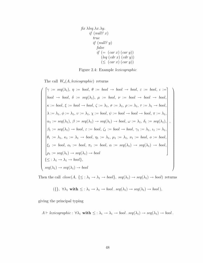
fix λleq .λx.λy.if (null? x)

trueif (null? y)

falseif (= (car x) (car y))

(leq (cdr x) (cdr y))(≤ (car x) (car y))

Figure 2.4: Example lexicographic

The call Wo(A, lexicographic) returns

γ := seq(λ1), η := bool , θ := bool → bool → bool , ε := bool , ι :=

bool → bool , δ := seq(λ1), µ := bool , ν := bool → bool → bool ,

κ := bool , ξ := bool → bool , ζ := λ1, σ := λ1, ρ := λ1, τ := λ1 → bool ,

λ := λ1, φ := λ1, υ := λ1, χ := bool , ψ := bool → bool → bool , π := λ1,

α1 := seq(λ1), β := seq(λ1) → seq(λ1) → bool , ω := λ1, δ1 := seq(λ1),

β1 := seq(λ1) → bool , ε := bool , ζ1 := bool → bool , γ1 := λ1, ι1 := λ1,

θ1 := λ1, κ1 := λ1 → bool , η1 := λ1, µ1 := λ1, ν1 := bool , o := bool ,

ξ1 := bool , o1 := bool , π1 := bool , α := seq(λ1) → seq(λ1) → bool ,

ρ1 := seq(λ1)→ seq(λ1)→ bool

,

{≤ : λ1 → λ1 → bool},

seq(λ1)→ seq(λ1)→ bool

Then the call close(A, {≤ : λ1 → λ1 → bool}, seq(λ1)→ seq(λ1)→ bool) returns

({}, ∀λ1 with ≤ : λ1 → λ1 → bool . seq(λ1)→ seq(λ1)→ bool ),

giving the principal typing

A ⊢ lexicographic : ∀λ1 with ≤ : λ1 → λ1 → bool . seq(λ1)→ seq(λ1)→ bool .

48

2.4 Properties of Wo

2.4.1 Soundness of Wo

First we have a lemma giving the properties needed of close in proving that Wo

is sound.

Lemma 2.17 If (B′, σ) = close(A,B, τ) succeeds, then for any e , if A∪B ⊢ e : τ

then A ∪ B′ ⊢ e : σ . Also, every identifier occurring in B′ or in the constraints

of σ occurs in B .

Proof: Suppose that (B′, σ) = close(A,B, τ) succeeds and that A ∪ B ⊢ e : τ .

There are two cases to consider:

1. A has no free type variables.

In this case satisfiable(B,A) is true, so there exists a substitution S such

that A ⊢ BS . The only variables occurring in B are the α , so we may

write S = [α := π] without loss of generality. Since B′′ ⊆ B , we have

A ⊢ B′′[α := π] and A ⊢ (B − B′′)[α := π] . Now by the definition of B′′ ,

the α do not occur in B − B′′ , so in fact we have A ⊢ B − B′′ . Then, by

Corollary 2.11, we have A∪B′′ ⊢ B−B′′ . Since A∪B′′ ∪ (B−B′′) ⊢ e : τ ,

we may apply Corollary 2.12 to yield A∪B′′ ⊢ e : τ . The α are by definition

not free in A , so (∀ -intro) may be applied:

A ∪B′′ ⊢ e : τ

A ⊢ B′′[α := π]

A ⊢ e : ∀α with B′′ . τ

showing that A ∪B′ ⊢ e : σ .

2. A has free type variables.

49

Let β be new type variables not occurring in A , B , or τ . By Lemma 2.4, we

have (A∪B)[α := β] ⊢ e : τ [α := β] . Then by Corollary 2.14, (A∪B)[α :=

β] ∪B ⊢ e : τ [α := β] . Now (A ∪B)[α := β] ∪B = A ∪B ∪B′′[α := β] , by

the definitions of α and B′′ . Hence ( ∀ -intro) may be applied:

A ∪ B ∪ B′′[α := β] ⊢ e : τ [α := β]

A ∪ B ⊢ B′′[α := β][β := α]

A ∪ B ⊢ e : ∀β with B′′[α := β] . τ [α := β]

since the β are not free in A ∪B . Finally, since

∀β with B′′[α := β] . τ [α := β] ≡α ∀α with B′′ . τ ,

we may use (≡α ) to get A ∪B ⊢ e : ∀α with B′′ . τ .

As for the second part of the lemma, it follows immediately from the fact that

B′ and B′′ are subsets of B . QED

Theorem 2.18 If (S,B, τ) = Wo(A, e) succeeds, then AS ∪ B ⊢ e : τ . Fur-

thermore, every identifier occurring in B is overloaded in A or occurs in some

constraint of some assumption in A .

Proof: By induction on the structure of e .

1. e is x

Then Wo(A, e) is defined as:

if x is overloaded in A with lcg ∀α.τ ,

return ([ ], {x : τ [α := β]}, τ [α := β]) where β are new

else if (x : ∀α with C . τ ) ǫ A ,

return ([ ], C[α := β], τ [α := β]) where β are new

else fail.

50

If x is overloaded in A , then (S,B, τ) = ([ ], {x : τ [α := β]}, τ [α := β]) , so

AS ∪ B = A ∪ {x : τ [α := β]} . So by (hypoth), AS ∪ B ⊢ x : τ [α := β] .

Also, every identifier occurring in B is overloaded in A .

If x is not overloaded in A , then (S,B, τ) = ([ ], C[α := β], τ [α := β]) ,

so AS ∪ B = A ∪ C[α := β] . By (hypoth), AS ∪ B ⊢ x : ∀α with C . τ

and AS ∪ B ⊢ C[α := β] . So by a (possibly trivial) use of ( ∀ -elim),

AS ∪ B ⊢ x : τ [α := β] . Also, every identifier occurring in B occurs in a

constraint of an assumption in A .

2. e is λx.e′


if x occurs in A , fail.

let (S1, B1, τ1) = Wo(A ∪ {x : α}, e′) where α is new;

return (S1, B1, αS1 → τ1) .

By induction, (A ∪ {x : α})S1 ∪ B1 ⊢ e′ : τ1 . Also, every identifier in B1 is

overloaded in A ∪ {x : α} or occurs in some constraint of some assumption

in A ∪ {x : α} . Since x does not occur in A , and since the type α has

no constraints, this means that every identifier in B1 is overloaded in A or

occurs in some constraint of some assumption in A . In particular, x does

not occur in B1 and, therefore, x does not occur in AS1 ∪ B1 . So, since

(A ∪ {x : α})S1 ∪ B1 = AS1 ∪ B1 ∪ {x : αS1} , we can use (→ -intro) to get

AS1 ∪B1 ⊢ λx.e′ : αS1 → τ1 .

3. e is e′e′′


51

let (S1, B1, τ1) = Wo(A, e′) ;

let (S2, B2, τ2) = Wo(AS1, e′′) ;

let S3 = unify(τ1S2, τ2 → α) where α is new;

return (S1S2S3, B1S2S3 ∪B2S3, αS3) .

By induction, AS1 ∪ B1 ⊢ e′ : τ1 and AS1S2 ∪ B2 ⊢ e′′ : τ2 , and every

identifier occurring in B1 or in B2 is overloaded in A or occurs in some

constraint of some assumption in A . Hence every identifier occurring in

B1S2S3 ∪ B2S3 is overloaded in A or occurs in some constraint of some

assumption in A . By Lemma 2.4, AS1S2S3 ∪ B1S2S3 ⊢ e′ : τ1S2S3 and

AS1S2S3 ∪ B2S3 ⊢ e′′ : τ2S3 . So by Corollary 2.14,

AS1S2S3 ∪ B1S2S3 ∪B2S3 ⊢ e′ : τ1S2S3

and

AS1S2S3 ∪ B1S2S3 ∪ B2S3 ⊢ e′′ : τ2S3.

By the definition of unify, τ1S2S3 = τ2S3 → αS3 . Hence by (→ -elim), we

have

AS1S2S3 ∪ B1S2S3 ∪ B2S3 ⊢ e′e′′ : αS3.




let (S1, B1, τ1) = Wo(A, e′) ;

let (B′

1, σ1) = close(AS1, B1, τ1) ;

let (S2, B2, τ2) = Wo(AS1 ∪ {x : σ1}, e′′) ;

return (S1S2, B′

1S2 ∪B2, τ2) .

By induction, AS1 ∪ B1 ⊢ e′ : τ1 , and every identifier occurring in B1 is

overloaded in A or occurs in some constraint of some assumption in A .

52

So by Lemma 2.17, AS1 ∪ B′1 ⊢ e′ : σ1 and every identifier occurring in

B′1 is overloaded in A or occurs in some constraint of some assumption in

A . In particular, since x does not occur in A , x does not occur in B′1 .

Also by induction, (AS1 ∪ {x : σ1})S2 ∪ B2 ⊢ e′′ : τ2 , which is the same as

AS1S2 ∪ B2 ∪ {x : σ1S2} ⊢ e′′ : τ2 , and every identifier occurring in B2 is

overloaded in AS1∪{x : σ1} or occurs in some constraint of some assumption

in AS1 ∪ {x : σ1} . Now x does not occur in A , and by Lemma 2.17 every

identifier occurring in the constraints of σ1 occurs in B1 . Hence every

identifier occurring in B2 is overloaded in A or occurs in some constraint of

some assumption in A . In particular, then, x does not occur in B2 . Now

Lemma 2.4 and Corollary 2.14 may be applied to give

AS1S2 ∪ B′1S2 ∪ B2 ⊢ e

′ : σ1S2

and

AS1S2 ∪ B′1S2 ∪B2 ∪ {x : σ1S2} ⊢ e

′′ : τ2.

So, since x does not occur in AS1S2 ∪ B′1S2 ∪B2 , (let) may be used to get

AS1S2 ∪ B′1S2 ∪B2 ⊢ let x = e′ in e′′ : τ2.

QED

2.4.2 Completeness of Wo

Ultimately, we will prove the following principal typing result.

Theorem Let A be an assumption set with satisfiable constraints and no free type

variables. If e is well typed with respect to A , then (S,B, τ) = Wo(A, e) succeeds,

(B′, σ) = close(A,B, τ) succeeds, and the typing A ⊢ e : σ is principal.

53

Reaching this result will take some time, however.

We start with a lemma that gives the properties of close needed to establish

the completeness of Wo .

Lemma 2.19 If AS ⊢ BS , then (B′, σ) = close(A,B, τ) succeeds and σ is of

the form ∀α with B′′ . τ . In addition,

• if A has no free type variables then B′ = {} ,

• fv(σ) ⊆ fv(A) , and

• B′ ∪ B′′ ⊆ B .

Proof: If A has free type variables, then close(A,B, τ) succeeds. If A has

no free type variables, then the assumption AS ⊢ BS becomes A ⊢ BS . Hence

satisfiable(B,A) is true, and close(A,B, τ) succeeds.

The remaining parts of the lemma are immediate from the definition of close(A,B, τ) .

QED

Lemma 2.20 If (S,B, τ) = Wo(A, e) succeeds, then every type variable occurring

in S , B , or τ occurs free in A or else is generated by the new type variable

generator.

Proof: A straightforward induction on the structure of e , using properties of

unify and Lemma 2.19. QED

Definition 2.4 Let A and A′ be assumption sets. We say that A is stronger

than A′ , written A � A′ , if

1. A′ ⊢ x : τ implies A ⊢ x : τ , and

2. id(A) ⊆ id(A′) .

54

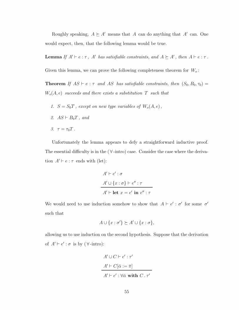
Roughly speaking, A � A′ means that A can do anything that A′ can. One

would expect, then, that the following lemma would be true.

Lemma If A′ ⊢ e : τ , A′ has satisfiable constraints, and A � A′ , then A ⊢ e : τ .

Given this lemma, we can prove the following completeness theorem for Wo :

Theorem If AS ⊢ e : τ and AS has satisfiable constraints, then (S0, B0, τ0) =

Wo(A, e) succeeds and there exists a substitution T such that

1. S = S0T , except on new type variables of Wo(A, e) ,

2. AS ⊢ B0T , and

3. τ = τ0T .

Unfortunately the lemma appears to defy a straightforward inductive proof.

The essential difficulty is in the (∀ -intro) case. Consider the case where the deriva-

tion A′ ⊢ e : τ ends with (let):

A′ ⊢ e′ : σ

A′ ∪ {x : σ} ⊢ e′′ : τ

A′ ⊢ let x = e′ in e′′ : τ

We would need to use induction somehow to show that A ⊢ e′ : σ′ for some σ′

such that

A ∪ {x : σ′} � A′ ∪ {x : σ},

allowing us to use induction on the second hypothesis. Suppose that the derivation

of A′ ⊢ e′ : σ is by ( ∀ -intro):

A′ ∪ C ⊢ e′ : τ ′

A′ ⊢ C[α := π]

A′ ⊢ e′ : ∀α with C . τ ′

55

Now we would like to use induction to show that A ∪ C ⊢ e′ : τ ′ . But we have a

serious problem: it need not be the case that A∪C � A′∪C ! And in fact, it need

not be the case that A ∪ C ⊢ e′ : τ ′ . For example, let A = {x : int , y : int} and

A′ = {x : ∀α with y : α . α , y : int} . Then A � A′ . But A ∪ {y : β} 6� A′ ∪ {y :

β} , and also A ∪ {y : β} 6⊢ x : β although A′ ∪ {y : β} ⊢ x : β .

The point is that the derivation of A ⊢ e : τ may have to have a very different

structure from the derivation of A′ ⊢ e : τ , so it does not seem possible to ‘locally’

modify the derivation of A′ ⊢ e : τ to arrive at a derivation of A ⊢ e : τ . How,

then, can we find a derivation of A ⊢ e : τ ? The answer is to use Wo to find it.

But we haven’t yet shown the completeness of Wo , and indeed the whole reason

for introducing the lemma above was to prove the completeness theorem! So it

appears necessary to combine the lemma and theorem above into a single theorem

that yields both as corollaries and that allows both to be proved simultaneously.

We shall now do this.

Theorem 2.21 Suppose A′ ⊢ e : τ , A′ has satisfiable constraints, and AS � A′ .

Then (S0, B0, τ0) = Wo(A, e) succeeds and there exists a substitution T such that


2. AS ⊢ B0T , and

3. τ = τ0T .

Proof: By induction on the structure of e . By Theorem 2.9, A′ ⊢′ e : τ .

• e is x

By the definition of AS � A′ , we have AS ⊢′ x : τ . The last (non-trivial)

step of this derivation is either (hypoth) or ( ∀ -elim ′ ); we may write the

derivation so that the last step is a (possibly trivial) use of ( ∀ -elim ′ ). If

56

(x : ∀α with C . ρ ) ǫ A , then (x : ∀β with C[α := β]S . ρ[α := β]S ) ǫ AS ,

where β are the first distinct type variables not free in ∀α with C . ρ or

in S . Hence the derivation AS ⊢′ x : τ ends with

(x : ∀β with C[α := β]S . ρ[α := β]S) ǫ AS

AS ⊢′ C[α := β]S[β := π]

AS ⊢′ x : ρ[α := β]S[β := π]

where ρ[α := β]S[β := π] = τ .

We need to show that (S0, B0, τ0) = Wo(A, x) succeeds and that there exists

T such that

1. S = S0T , except on new type variables of Wo(A, x) ,

2. AS ⊢ B0T , and

3. τ = τ0T .

Now, Wo(A, x) is defined by





else fail.

If x is overloaded in A with lcg ∀γ.ρ0 , then (S0, B0, τ0) = Wo(A, x) suc-

ceeds with S0 = [ ] , B0 = {x : ρ0[γ := δ]} , and τ0 = ρ0[γ := δ] , where δ are

new. Since ∀γ.ρ0 is the lcg of x , γ are the only variables in ρ0 and there

exist φ such that ρ0[γ := φ] = ρ . Let T be S ⊕ [δ := φ[α := β]S[β := π]] .

57

Then

τ0T

= ≪ definition≫

ρ0[γ := δ](S ⊕ [δ := φ[α := β]S[β := π]]

= ≪ only δ occur in ρ0[γ := δ]≫

ρ0[γ := δ][δ := φ[α := β]S[β := π]]

= ≪ only γ occur in ρ0 ≫

ρ0[γ := φ[α := β]S[β := π]]


ρ0[γ := φ][α := β]S[β := π]

= ≪ by above≫

ρ[α := β]S[β := π]

= ≪ by above≫

τ.

So

1. S0T = S ⊕ [δ := φ[α := β]S[β := π]] = S , except on δ . That is,

S0T = S , except on the new type variables of Wo(A, x) .

2. Since B0T = {x : τ0T} = {x : τ} , it follows that AS ⊢ B0T .

3. τ0T = τ .

If x is not overloaded in A , then (S0, B0, τ0) = Wo(A, x) succeeds with

S0 = [ ] , B0 = C[α := δ] , and τ0 = ρ[α := δ] , where δ are new. Observe

that [α := δ](S ⊕ [δ := π]) and [α := β]S[β := π] agree on C and on ρ .

(The only variables in C or ρ are the α and variables ε not

among β or δ . Both substitutions map αi 7→ πi and ε 7→ εS .)

Let T be S ⊕ [δ := π] . Then

58

1. S0T = S ⊕ [δ := π] = S , except on δ . That is, S0T = S , except on

the new type variables of Wo(A, x) .

2. Also,

B0T

= ≪ definition≫

C[α := δ](S ⊕ [δ := π])

= ≪ by above observation≫

C[α := β]S[β := π].

Hence AS ⊢ B0T .

3. Finally,

τ0T

= ≪ definition≫

ρ[α := δ](S ⊕ [δ := π])


ρ[α := β]S[β := π]

=

τ.

• e is λx.e′

The last (non-trivial) step of the derivation of A′ ⊢′ e : τ must be (→ -intro):

A′ ∪ {x : τ ′} ⊢′ e′ : τ ′′

A′ ⊢′ λx.e′ : τ ′ → τ ′′

where x does not occur in A′ .

We must show that (S0, B0, τ0) = Wo(A, λx.e′) succeeds and that there exists

T such that

1. S = S0T , except on new type variables of Wo(A, λx.e′) ,

59

2. AS ⊢ B0T , and

3. τ ′ → τ ′′ = τ0T .

Now, Wo(A, λx.e′) is defined by


let (S1, B1, τ1) = Wo(A ∪ {x : α}, e′) where α is new;


Since x does not occur in A′ and (by AS � A′ ) id(AS) ⊆ id(A′) , it follows

that x does not occur in AS . This implies that x does not occur in A , so

the first line does not fail.

Now we wish to use induction to show that the recursive call succeeds. The

new type variable α is not free in A , so

AS ∪ {x : τ ′} = (A ∪ {x : α})(S ⊕ [α := τ ′]).

By Lemma 2.16, A′∪{x : τ ′} has satisfiable constraints. Next we argue that

AS ∪ {x : τ ′} � A′ ∪ {x : τ ′} . Clearly, id(AS ∪ {x : τ ′}) ⊆ id(A′ ∪ {x : τ ′}) .

Now suppose that A′ ∪ {x : τ ′} ⊢ y : ρ . If y 6= x , then by Corollary 2.10,

A′ ⊢ y : ρ . Since AS � A′ , we have AS ⊢ y : ρ and then by Corollary 2.11,

AS ∪ {x : τ ′} ⊢ y : ρ . On the other hand, if y = x , then the derivation

A′ ∪ {x : τ ′} ⊢′ y : ρ must be by (hypoth)—hence ρ = τ ′ . So by (hypoth),

AS ∪ {x : τ ′} ⊢ y : ρ . We have shown that

– A′ ∪ {x : τ ′} ⊢ e′ : τ ′′ ,

– A′ ∪ {x : τ ′} has satisfiable constraints, and

– (A ∪ {x : α})(S ⊕ [α := τ ′]) � A′ ∪ {x : τ ′} .

So by induction, (S1, B1, τ1) = Wo(A∪ {x : α}, e′) succeeds and there exists

T1 such that

60

1. S ⊕ [α := τ ′] = S1T1 , except on new variables of Wo(A ∪ {x : α}, e′) ,

2. (A ∪ {x : α})(S ⊕ [α := τ ′]) ⊢ B1T1 , and

3. τ ′′ = τ1T1 .

So (S0, B0, τ0) = Wo(A, λx.e′) succeeds with S0 = S1 , B0 = B1 , and

τ0 = αS1 → τ1 .

Let T be T1 . Then

1. Observe that

S0T

= ≪ definition≫

S1T1

= ≪ by part 1 of inductive hypothesis above≫

S ⊕ [α := τ ′], except on new variables of Wo(A ∪ {x : α}, e′)

= ≪ definition of ⊕ ≫

S, except on α.

Hence S0T = S , except on the new type variables of Wo(A∪{x : α}, e′)

and on α . That is, S0T = S , except on the new type variables of

Wo(A, λx.e′) .

2. B0T = B1T1 and we have AS ∪ {x : τ ′} ⊢ B1T1 . By Theorem 2.18,

every identifier occurring in B1 is overloaded in A ∪ {x : α} or occurs

in some constraint of some assumption in A ∪ {x : α} . Since x does

not occur in A and α has no constraints, this means that x does not

occur in B1 . Hence Corollary 2.10 may be applied to each member of

B1T1 , yielding

AS ⊢ B1T1.

61

3. Finally,

τ0T

= ≪ definition≫

(αS1 → τ1)T1

= ≪ by part 3 of the use of induction above≫

αS1T1 → τ ′′

= ≪ α is not a new variable of Wo(A ∪ {x : α}, e′)≫

α(S ⊕ [α := τ ′])→ τ ′′


τ ′ → τ ′′.

• e is e′e′′

The last (non-trivial) step of the derivation of A′ ⊢′ e : τ must be (→ -elim):

A′ ⊢′ e′ : τ ′ → τ

A′ ⊢′ e′′ : τ ′

A′ ⊢′ e′ e′′ : τ

We need to show that (S0, B0, τ0) = Wo(A, e′e′′) succeeds and that there

exists T such that

1. S = S0T , except on new type variables of Wo(A, e′e′′) ,

2. AS ⊢ B0T , and

3. τ = τ0T .

Now, Wo(A, e′e′′) is defined by

let (S1, B1, τ1) = Wo(A, e′) ;

let (S2, B2, τ2) = Wo(AS1, e′′) ;

let S3 = unify(τ1S2, τ2 → α) where α is new;

return (S1S2S3, B1S2S3 ∪B2S3, αS3) .

62

By induction, (S1, B1, τ1) = Wo(A, e′) succeeds and there exists T1 such

that

1. S = S1T1 , except on new type variables of Wo(A, e′) ,

2. AS ⊢ B1T1 , and

3. τ ′ → τ = τ1T1 .

Now AS = A(S1T1) = (AS1)T1 , as the new type variables of Wo(A, e′) do

not occur free in A . So by induction, (S2, B2, τ2) = Wo(AS1, e′′) succeeds

and there exists T2 such that

1. T1 = S2T2 , except on new type variables of Wo(AS1, e′′) ,

2. (AS1)T1 ⊢ B2T2 , and

3. τ ′ = τ2T2 .

By Lemma 2.20, the new variable α does not occur in A , S1 , B1 , τ1 , S2 ,

B2 , or τ2 . So consider T2 ⊕ [α := τ ] :

(τ1S2)(T2 ⊕ [α := τ ])

= ≪ α does not occur in τ1S2 ≫

τ1S2T2

= ≪ no new type variable of Wo(AS1, e′′) occurs in τ1 ≫

τ1T1

= ≪ by part 3 of first use of induction above≫

τ ′ → τ

63

In addition,

(τ2 → α)(T2 ⊕ [α := τ ])

= ≪ α does not occur in τ2 ≫

τ2T2 → τ

= ≪ by part 3 of second use of induction above≫

τ ′ → τ

Hence by Robinson’s unification theorem [Rob65], S3 = unify(τ1S2, τ2 → α)

succeeds and there exists T3 such that

T2 ⊕ [α := τ ] = S3T3.

So (S0, B0, τ0) = Wo(A, e′e′′) succeeds with S0 = S1S2S3 , B0 = B1S2S3 ∪

B2S3 , and τ0 = αS3 .

Let T be T3 . Then

1. Observe that

S0T

= ≪ definition≫

S1S2S3T3

= ≪ by above property of unifier S3 ≫

S1S2(T2 ⊕ [α := τ ])

= ≪ α does not occur in S1S2 ≫

S1S2T2, except on α

= ≪ by part 1 of second use of induction and since the≫

≪ new variables of Wo(AS1, e′′) don’t occur in S1 ≫

S1T1, except on the new type variables of Wo(AS1, e′′)

= ≪ by part 1 of the first use of induction above≫

S, except on the new type variables of Wo(A, e′).

64

Hence we see that S0T = S except on α , on the new type variables

of Wo(AS1, e′′) , and on the new type variables of Wo(A, e

′) . That is,

S0T = S except on the new type variables of Wo(A, e′e′′) .

2. Next,

B0T

= ≪ definition≫

B1S2S3T3 ∪ B2S3T3


B1S2(T2 ⊕ [α := τ ]) ∪B2(T2 ⊕ [α := τ ])

= ≪ α does not occur in B1S2 or in B2 ≫

B1S2T2 ∪B2T2


≪ new variables of Wo(AS1, e′′) don’t occur in B1 ≫

B1T1 ∪ B2T2

By part 2 of the first and second uses of induction above, AS ⊢ B1T1 ∪

B2T2 , and so AS ⊢ B0T .

3. Finally,

τ0T

= ≪ definition≫

αS3T3


α(T2 ⊕ [α := τ ])


τ

• e is let x = e′ in e′′

65

The last (non-trivial) step of the derivation of A′ ⊢′ e : τ must be (let):

A′ ⊢′ e′ : σ

A′ ∪ {x : σ} ⊢′ e′′ : τ

A′ ⊢′ let x = e′ in e′′ : τ


We need to show that (S0, B0, τ0) = Wo(A, let x = e′ in e′′ ) succeeds and

that there exists T such that

1. S = S0T , except on new type variables of Wo(A, let x = e′ in e′′ ) ,

2. AS ⊢ B0T , and

3. τ = τ0T .

Now, Wo(A, let x = e′ in e′′ ) is defined by


let (S1, B1, τ1) = Wo(A, e′) ;

let (B′

1, σ1) = close(AS1, B1, τ1) ;

let (S2, B2, τ2) = Wo(AS1 ∪ {x : σ1}, e′′) ;

return (S1S2, B′

1S2 ∪B2, τ2) .

Since AS � A′ , x does not occur in AS or in A . So the first line does not

fail.

Since A′ has satisfiable constraints, by Lemma 2.15 there exists τ ′ such that

A′ ⊢ e′ : τ ′ . Hence by induction, (S1, B1, τ1) = Wo(A, e′) succeeds and there

exists T1 such that


2. AS ⊢ B1T1 , and

3. τ ′ = τ1T1 .

66

By 1 and 2 above, we have (AS1)T1 ⊢ B1T1 , so by Lemma 2.19 it fol-

lows that (B′1, σ1) = close(AS1, B1, τ1) succeeds and σ1 is of the form

∀α with B′′1 . τ1 . Also fv(σ1) ⊆ fv(AS1) and B′

1 ∪B′′1 ⊆ B1 .

Now, in order to apply the induction hypothesis to the second recursive call

we need to show that

AS ∪ {x : σ1T1} � A′ ∪ {x : σ}.

There are two parts to this:

1. A′ ∪ {x : σ} ⊢ y : ρ implies AS ∪ {x : σ1T1} ⊢ y : ρ , and

2. id(AS ∪ {x : σ1T1}) ⊆ id(A′ ∪ {x : σ}) .

The second part is quite simple; we show it first. By Lemma 2.17 and

Theorem 2.18, id(σ1) ⊆ id(B1) ⊆ id(A) . Hence

id(AS ∪ {x : σ1T1})

= ≪ by above≫

id(AS) ∪ {x}

⊆ ≪ AS � A′ ≫

id(A′) ∪ {x}

⊆

id(A′ ∪ {x : σ}),

showing 2.

Now we show 1. Suppose that A′ ∪ {x : σ} ⊢ y : ρ . If y 6= x , then by

Corollary 2.10, A′ ⊢ y : ρ . Since AS � A′ , we have AS ⊢ y : ρ and then

by Corollary 2.11, AS ∪ {x : σ1T1} ⊢ y : ρ .

If, on the other hand, y = x , then our argument will begin by establishing

that A′ ⊢ e′ : ρ . By Theorem 2.9 we have A′ ∪ {x : σ} ⊢′ x : ρ and

67

the derivation ends with (hypoth) or ( ∀ -elim ′ ). If the derivation ends with

(hypoth), then σ = ρ and so A′ ⊢ e′ : ρ . If the derivation ends with ( ∀ -

elim ′ ), then σ is of the form ∀β with C . ρ′ and the derivation is of the

form

x :∀β with C . ρ′ ǫ A′ ∪ {x : σ}

A′ ∪ {x : σ} ⊢′ C[β := π]

A′ ∪ {x : σ} ⊢′ x : ρ′[β := π]

where ρ = ρ′[β := π] . It is evident that x does not occur in C (if x occurs

in C , then the derivation of A′ ∪ {x : σ} ⊢′ C[β := π] will be infinitely

high), so by Corollary 2.10 applied to each member of C[β := π] , it follows

that A′ ⊢ C[β := π] . Now the derivation A′ ⊢ e′ : ∀β with C . ρ′ may be

extended using (∀ -elim):

A′ ⊢ e′ : ∀β with C . ρ′

A′ ⊢ C[β := π]

A′ ⊢ e′ : ρ′[β := π],

giving that A′ ⊢ e′ : ρ .

So by induction there exists a substitution T2 such that


2. AS ⊢ B1T2 , and

3. ρ = τ1T2 .

The new type variables of Wo(A, e′) are not free in A , so AS1T1 = AS =

AS1T2 . Hence T1 and T2 are equal when restricted to the free variables of

AS1 . Since, by Lemma 2.19, fv(σ1) ⊆ fv(AS1) , it follows that σ1T1 = σ1T2 .

Now, σ1 is of the form ∀α with B′′1 . τ1 , so σ1T1 (= σ1T2) is of the form

∀γ with B′′1 [α := γ]T2 . τ1[α := γ]T2 ,

68

where γ are the first distinct type variables not free in T2 or σ1 .

Consider the substitution [γ := αT2] . We have

B′′1 [α := γ]T2[γ := αT2] = B′′

1T2

and

τ1[α := γ]T2[γ := αT2] = τ1T2.

By 2 above, we have AS ⊢ B1T2 . Since by Lemma 2.19 we have B′′1 ⊆ B1 ,

it follows that AS ⊢ B′′1T2 . By Corollary 2.11, then, we have AS ∪ {x :

σ1T1} ⊢ B′′1T2 . Hence we have the following derivation:

AS ∪ {x : σ1T1} ⊢ x : ∀γ with B′′1 [α := γ]T2 . τ1[α := γ]T2

by (hypoth) since σ1T1 = ∀γ with B′′1 [α := γ]T2 . τ1[α := γ]T2 ,

AS ∪ {x : σ1T1} ⊢ B′′1 [α := γ]T2[γ := αT2]

by above since B′′1 [α := γ]T2[γ := αT2] = B′′

1T2 , and hence

AS ∪ {x : σ1T1} ⊢ x : τ1T2,

by (∀ -elim) since τ1[α := γ]T2[γ := αT2] = τ1T2 . Since by 3 above, τ1T2 =

ρ , we have at last that

AS ∪ {x : σ1T1} ⊢ x : ρ.

This completes that proof that AS ∪ {x : σ1T1} � A′ ∪ {x : σ} , which is the

same as

(AS1 ∪ {x : σ1})T1 � A′ ∪ {x : σ}.

Because A′ ⊢ e′ : σ and A′ has satisfiable constraints, it is easy to see that

the constraints of σ are satisfiable with respect to A′ . Hence by Lemma 2.16,

A′ ∪ {x : σ} has satisfiable constraints.

69

This allows us to apply the induction hypothesis again, which shows that

(S2, B2, τ2) = Wo(AS1 ∪ {x : σ1}, e′′) succeeds and that there exists T3 such

that

1. T1 = S2T3 , except on the new type variables of Wo(AS1∪{x : σ1}, e′′) ,

2. AS ∪ {x : σ1T1} ⊢ B2T3 , and

3. τ = τ2T3 .

So (S0, B0, τ0) = Wo(A, let x = e′ in e′′ ) succeeds with S0 = S1S2 , B0 =

B′1S2 ∪ B2 , and τ0 = τ2 .

Let T be T3 . Then

1. Observe that

S0T

= ≪ definition≫

S1S2T3

= ≪ part 1 of third use of induction; the new variables≫

≪ of Wo(AS1 ∪ {x : σ1}, e′′) don’t occur in S1 ≫

S1T1, except on new type variables of Wo(AS1 ∪ {x : σ1}, e′′)

= ≪ by part 1 of first use of induction above≫

S, except on new type variables of Wo(A, e′).

So S0T = S , except on new variables of Wo(A, let x = e′ in e′′ ) .

70

2. Next,

B0T

= ≪ definition≫

B′1S2T3 ∪ B2T3

⊆ ≪ Lemma 2.19≫

B1S2T3 ∪ B2T3


≪ of Wo(AS1 ∪ {x : σ1}, e′′) don’t occur in B1 ≫

B1T1 ∪B2T3

Now by part 2 of the first use of induction above, AS ⊢ B1T1 . And by

part 2 of the third use of induction above, AS ∪ {x : σ1T1} ⊢ B2T3 .

By Theorem 2.18, every identifier occurring in B1 is overloaded in A

or occurs in some constraint of some assumption in A . Since x does

not occur in A , it follows that x does not occur in B1 either. Now by

Lemma 2.19, the constraints of σ1 are a subset of B1 . Hence x does

not occur in the constraints of σ1 . By Theorem 2.18, every identifier

occurring in B2 is overloaded in AS1 ∪ {x : σ1} or occurs in some

constraint of some assumption in AS1 ∪ {x : σ1} . Since x does not

occur in AS1 or in the constraints of σ1 , it follows that x does not

occur in B2 . Hence Corollary 2.10 may be applied to each member of

B2T3 , yielding AS ⊢ B2T3 . So AS ⊢ B0T .

71

3. Finally,

τ0T

= ≪ definition≫

τ2T3

= ≪ by part 3 of the third use of induction above≫

τ.

QED

At long last, we get the completeness of Wo as a simple corollary:

Corollary 2.22 If AS ⊢ e : τ and AS has satisfiable constraints, then

(S0, B0, τ0) = Wo(A, e) succeeds and there exists a substitution T such that


2. AS ⊢ B0T , and

3. τ = τ0T .

Proof: Follows immediately from Theorem 2.21 by letting A′ be AS , and noting

that � is reflexive. QED

Also, we can now prove the stubborn � -lemma:

Corollary 2.23 If A′ ⊢ e : τ , A′ has satisfiable constraints, and A � A′ , then

A ⊢ e : τ .

Proof: Letting S be [ ] , we see from Theorem 2.21 that (S0, B0, τ0) = Wo(A, e)

succeeds and there exists a substitution T such that

1. [ ] = S0T , except on new type variables of Wo(A, e) ,

2. A ⊢ B0T , and

72

3. τ = τ0T .

Now by Theorem 2.18, AS0∪B0 ⊢ e : τ0 , so by Lemma 2.4, AS0T ∪B0T ⊢ e : τ0T .

Using 1 and 3 above, this gives us A ∪ B0T ⊢ e : τ . Since by 2 above A ⊢ B0T ,

we may use Corollary 2.12 to show that A ⊢ e : τ . QED

Finally, we obtain as a corollary the following principal typing result:

Corollary 2.24 Let A be an assumption set with satisfiable constraints and no

free type variables. If e is well typed with respect to A , then (S,B, τ) = Wo(A, e)

succeeds, (B′, σ) = close(A,B, τ) succeeds, and the typing A ⊢ e : σ is principal.

Proof: Since e is well typed with respect to A and since A has satisfiable

constraints, by Lemma 2.15 there exists π such that A ⊢ e : π . Hence we see

from Corollary 2.22 that (S,B, τ) = Wo(A, e) succeeds and there exists T such

that

1. [ ] = ST , except on the new type variables of Wo(A, e) ,

2. A ⊢ BT , and

3. π = τT .

Since AT ⊢ BT , by Lemma 2.19 (B′, σ) = close(A,B, τ) succeeds, σ is of the

form ∀α with B′′ . τ , and

• B′ = {} ,

• σ has no free type variables, and

• B′′ ⊆ B .

By Theorem 2.18 and Lemma 2.17, we have A ⊢ e : σ .

Now let σ′ be an arbitrary type scheme such that A ⊢ e : σ′ . We need to show

that σ ≥A σ′ . Suppose that σ′ ≥A ρ . Then by the definition of ≥A it follows

73

that (∀ -elim) may be used to derive A ⊢ e : ρ . So by Corollary 2.22 again, there

exists T ′ such that

1. [ ] = ST ′ , except on the new type variables of Wo(A, e) ,

2. A ⊢ BT ′ , and

3. ρ = τT ′ .

Since B′′ ⊆ B , we have A ⊢ B′′T ′ . Notice also that all of the variables occurring

in B′′ or in τ are among the α , so by restricting T ′ to the α we obtain a

substitution [α := φ] such that A ⊢ B′′[α := φ] and ρ = τ [α := φ] . This

shows that ∀α with B′′ . τ ≥A ρ , and hence that ∀α with B′′ . τ ≥A σ′ . So

A ⊢ e : ∀α with B′′ . τ is principal. QED

2.5 Limitative Results

Recall that in our definition of close(A,B, τ) in Section 2.3, we made use of

a function satisfiable(B,A) without indicating how it might be computed. We

address that omission in this section.

Given a set B of τ -assumptions and an assumption set A , satisfiable(B,A)

returns true if B is satisfiable with respect to A (that is, if there exists a sub-

stitution S such that A ⊢ BS ) and returns false otherwise. Unfortunately, the

satisfiability problem turns out to be undecidable.

Theorem 2.25 Given an assumption set A and a set B of τ -assumptions, it is

undecidable whether B is satisfiable with respect to A .

Proof: It is easy to reduce the Post Correspondence Problem (PCP) [HU79]

to the satisfiability problem. We present the reduction by means of an example.

74

Suppose we are given the PCP instance

x1 = 10 y1 = 101

x2 = 011 y2 = 11

x3 = 110 y3 = ε,

where ε denotes the empty string. We will use type constants 0, 1, and $ and a

right-associative binary type constructor → . Define

Apcp =

p : (1→ 0)→ (1→ 0→ 1),

p : (0→ 1→ 1)→ (1→ 1),

p : (1→ 1→ 0→ $)→ $,

p : ∀α, β with p : α→ β . (1→ 0→ α)→ (1→ 0→ 1→ β),

p : ∀α, β with p : α→ β . (0→ 1→ 1→ α)→ (1→ 1→ β),

p : ∀α, β with p : α→ β . (1→ 1→ 0→ α)→ β

Now consider whether {p : α→ α} is satisfiable with respect to Apcp .

This will be true if and only if there is some τ such that Apcp ⊢ p : τ → τ .

But Apcp gives p precisely all types of the form π → π′ , where π is obtained by

concatenating various xi ’s and π′ is obtained by concatenating the corresponding

yi ’s.9 Hence {p : α → α} is satisfiable with respect to Apcp precisely when the

given PCP instance has a solution. QED

It is conceivable that there is some way to do type inference without using

function satisfiable(B,A) , but such hopes are quickly dashed by the following

corollary.

Corollary 2.26 Given an assumption set A and an expression e , it is undecid-

able whether e is well typed with respect to A .

Proof: Again we use a reduction from PCP. Define Apcp as above, and consider

whether the expression (λf.λx.f(f x)) p is well typed with respect to Apcp .9Possibly π and π′ have a $ tacked on the end.

75

Now, λf.λx.f(f x) has principal type ∀α.(α → α) → (α → α) . Hence

(λf.λx.f(f x))p is well typed with respect to Apcp if and only if p has some type

of the form τ → τ , which in turn holds if and only if the given PCP instance has

a solution.10 QED

Another easy corollary is that the instance relation ≥A is undecidable.

Corollary 2.27 Given A , σ , and τ , it is undecidable whether σ ≥A τ .

Proof: Define Apcp as above; then

∀α with p : α→ α . bool ≥Apcp bool

if and only if the given PCP instance has a solution. QED

It might appear that the key to all of these undecidability results is the necessity

of ‘guessing’: for example, to determine whether {p : α → α} is satisfiable we

must guess how α should be instantiated. This suggests that if we arrange to

eliminate such guessing, perhaps undecidability will be avoided.

To this end, we can define the class of coupled type schemes: a type scheme

∀α with C . τ is said to be coupled if every type variable occurring in C occurs

also in τ . For example, the type ∀α with p : α→ α . bool used in the proof of

Corollary 2.27 is uncoupled. We furthermore say that an assumption set A is

coupled if it contains only coupled assumptions.

We also require the notion of a nonoverlapping assumption set. We say that

type schemes σ and σ′ overlap if (after renaming to eliminate any common bound

type variables) their bodies are unifiable. Then we say that an assumption set A

is nonoverlapping if A contains no two assumptions x : σ and x : σ′ with σ and

σ′ overlapping.10We remark in passing that the expression (λf.λx.f(f x))p cannot be replaced by the simpler

expression λx.p(p x) in this proof. The problem with the simpler expression is that the twooccurrences of p are not forced to have the same type.

76

Finally we say that a type τ is ground if it contains no occurrences of type

variables, and an assumption x : τ is ground if τ is ground.

If A is coupled and nonoverlapping and B contains only ground assumptions,

then no guessing is involved in verifying the satisfiability of B with respect to A—

since B contains only ground assumptions, B is satisfiable if and only if A ⊢ B ,

and we can verify A ⊢ B by “working backwards” in a completely deterministic

manner. For example, if

A = {c : char , c : ∀α with c : α . seq(α) }

then we can reason

A ⊢ {c : seq(seq(char))}

m

A ⊢ {c : seq(char)}

m

A ⊢ {c : char}.

More formally, we can verify that A ⊢ B as follows:

while B 6= {} do

choose x : τ in B ;

find an assumption x : ∀α with C . ρ in A

such that for some S , ρS = τ ;

if none, then answer ‘no’;

B := (B − {x : τ}) ∪ CS ;

od;

answer ‘yes’.

Because of the restriction to nonoverlapping and coupled assumptions, there is

always a unique assumption to apply next, and B always contains only ground

assumptions. Notice, however, that if A = {c : ∀α with c : seq(α) . α } , then an

77

infinite branch will be generated when we attempt to verify that A ⊢ {c : char} ,

so our procedure is not guaranteed to terminate. One might imagine that such

infinite branches can somehow be detected and avoided, but, surprisingly, this is

not so.

Theorem 2.28 Given a coupled, nonoverlapping assumption set A and a ground

assumption x : τ , it is undecidable whether A ⊢ x : τ .

Proof: We reduce the problem of determining whether a deterministic Turing

Machine halts on empty input [HU79] to this problem. Suppose we are given a

Turing Machine M = (Q, {0, 1}, {0, 1, B}, δ, q0, B, {qH}) , where

• Q is the set of states,

• {0, 1} is the input alphabet,

• {0, 1, B} is the tape alphabet,

• δ : Q× {0, 1, B} → Q× {0, 1, B} × {L,R} ,

• q0 is the start state,

• B is the blank symbol,

• qH is the unique halting state.

The idea is to encode instantaneous descriptions (IDs) of M as types and to define

a set of type assumptions Ahalt so that Ahalt ⊢ h : ρ if and only if ρ encodes an

ID from which M eventually halts. We need just one identifier h , a binary type

constructor → , and a set of type constants Q ∪ {0, 1, B, ε} .

We encode IDs as follows: 01Bq10 is encoded as

(B → 1→ 0→ ε)→ q → (1→ 0→ ε),

78

and in general, for α1 and α2 in {0, 1, B}∗ , α1qα2 is encoded as

αreverse1 → q → α2,

where if α = X1X2 . . .Xn , n ≥ 0 , then α = X1 → X2 → · · · → Xn → ε .

Next, we observe that M eventually halts from ID if and only if either

• ID is a halting ID, or

• M eventually halts from the successor of ID .

We include assumptions in Ahalt to deal with these two possibilities. First, to

deal with halting IDs, we include

h : ∀α, β.α→ qH → β.

Next we want to express “ h : ID if h : successor( ID )”. Suppose that δ(q,X) =

(q′, Y, R) . We model this by including

h : α→ q → (X → β) if h : (Y → α)→ q′ → β,

which in our official syntax is

h : ∀α, β with h : (Y → α)→ q′ → β . α→ q → (X → β) .

In addition, if X = B then we also include

h : α→ q → ε if h : (Y → α)→ q′ → ε.

Similarly, if δ(q,X) = (q′, Y, L) , then for each Z in the tape alphabet we include

h : (Z → α)→ q → (X → β) if h : α→ q′ → (Z → Y → β)

and, if X = B ,

h : (Z → α)→ q → ε if h : α→ q′ → (Z → Y → ε).

79

It follows, then, that Ahalt ⊢ h : ε → q0 → ε if and only if M halts on ε .

Furthermore, Ahalt is coupled and nonoverlapping. QED

In Section 2.6 we present a set of restrictions that do make the satisfiability

problem decidable. First, however, we digress to mention an application of Theo-

rem 2.28 to logic and logic programming.

2.5.1 A Logical Digression

As we remarked earlier, our type assumptions can be rephrased as Horn clauses

[Llo87]. For each identifier x , we introduce a unary predicate symbol Tx with the

intention that Tx(τ) means x : τ . Then the type assumption

x : ∀α with x : α, y : α→ α . set(α)

is represented by the Horn clause

Tx(set(α))← Tx(α) ∧ Ty(α→ α).

The essential property of the translation is this: if A∗ denotes the translation of

A , then

A ⊢ x : τ

if and only if

A∗ ∪ {false← Tx(τ)} is unsatisfiable.

Furthermore, our definitions of coupled and nonoverlapping can be applied in the

obvious way to Horn clauses. So we have the following corollary to Theorem 2.28.

Corollary 2.29 It is undecidable whether a set of coupled, nonoverlapping Horn

clauses is satisfiable.

80

This corollary has consequences for logic programming as well: the set of all

logic programs that never require backtracking in their execution includes the

class of all sets of coupled, nonoverlapping Horn clauses. Hence the possibility of

nontermination cannot be avoided in logic programming, even in situations where

no backtracking can arise.

2.6 Restricted Forms of Overloading

In this section, we impose restrictions on the forms of overloading allowed; our

goal is to make the satisfiability problem decidable, which in turn will make the

typability problem decidable.

We saw in Section 2.5 that our assumption sets are expressive enough to encode

the Post Correspondence Problem and the Halting Problem. But the examples of

overloading that we care about in practice do not require nearly so much power.

Consider the assumptions for ≤ , our typical interesting example of overloading:




≤ : ∀α, β with ≤ : α→ α→ bool , ≤ : β → β → bool .

(α× β)→ (α× β)→ bool

The effect of these assumptions may be stated thus: the types of ≤ are of the

form τ → τ → bool ; by the first rule τ may be char , by the second rule τ may

be real , by the third rule τ may be seq(τ ′) if τ may be τ ′ , and by the fourth

rule τ may be τ ′×τ ′′ if τ may be τ ′ and τ ′′ . That is, ≤ has exactly those types

of the form τ → τ → bool where τ is any type built from the constructors real ,

char , seq , and × . In this situation, we can do better than our usual implicit

81

representation of the types for ≤ ; in fact we could use the explicit representation

∀α{char ,real ,seq ,×}

.α→ α→ bool ,

associating the constructor set {char , real , seq ,×} with α to express the fact that

α may only be instantiated with types built from those constructors. Furthermore,

we will see that this explicit representation of the types of ≤ is very useful in

solving the satisfiability problem. We now make these ideas precise.

Definition 2.5 We say that x is overloaded by constructors in A if the lcg of x

in A is of the form ∀α.τ and if for every assumption x : ∀β with C . ρ in A ,

• ρ = τ [α := χ(β)] , for some type constructor χ , and

• C = {x : τ [α := βi] | βiǫβ} .

Furthermore, we say that the type constructor set of x in A is

{χ | A contains an assumption x : ∀β with C . τ [α := χ(β)] }

For example, under the assumptions given above, ≤ is overloaded by constructors

and has type constructor set {char , real , seq ,×} .

Lemma 2.30 If x is overloaded by constructors in A with lcg ∀α.τ and type

constructor set X , then A ⊢ x : ρ if and only if ρ is of the form τ [α := π] and

π is a type built from the constructors in X .

Proof: The ‘if’ direction is a straightforward induction on the structure of π .

The ‘only if’ direction is a straightforward induction on the length of the deriva-

tion of A ⊢′ x : ρ . QED

Definition 2.6 We say that A is an overloading by constructors if

82

• every identifier overloaded in A is overloaded by constructors and

• for every constraint x : ρ in an assumption in A , x is overloaded in A and

ρ is an instance of the lcg of x .

We now argue that if A is an overloading by constructors, then the satis-

fiability problem can be solved efficiently. For simplicity, however, we restrict

satisfiable(B,A) to constraint sets B generated by Wo ; this is justified by the

fact that close calls satisfiable only on constraint sets generated by Wo . Now, if

A is an overloading by constructors, then a simple inductive argument shows that

if (S,B, τ) = Wo(A, e) , then B contains only constraints of the form x : ρ where

x is overloaded in A and ρ is an instance of the lcg of x . Hence we restrict our

attention to constraint sets of this form.

Let B be a constraint set containing only constraints of the form x : ρ where

x is overloaded in A and ρ is an instance of the lcg of x . Let x : ρ be a con-

straint in B . By assumption, ρ = τx[α := π] where ∀α.τx is the lcg of x in A ,

so by Lemma 2.30, A ⊢ x : ρS if and only if πS is a type constructed from Xx ,

the type constructor set of x . Examine π ; if it contains any type constructor

not in Xx , then B is unsatisfiable. Otherwise, S satisfies x : ρ if and only if S

instantiates all variables in π to types constructed from the constructors in Xx .

In this way, the constraint x : ρ in B associates the constructor set Xx with

each variable occurring in ρ . Now, for each variable β in B , take the intersection

of all the constructor sets thus associated with β ; this gives explicitly the set of

possible instantiations of β that satisfy B—in particular, there is some satisfying

instantiation of β if and only if the intersection contains a 0-ary type construc-

tor. Hence, B is satisfiable if and only if every variable in B has an associated

constructor set containing a 0-ary type constructor. Clearly, this procedure can be

done in polynomial time.

83

There is a natural example of overloading for which the restriction to overload-

ing by constructors is too severe. The example, due to Dennis Volpano, is matrix

multiplication: for matrices to be multiplied it is necessary that the elements of

the matrices can be multiplied and also added, for we need to form inner products.

Hence we would like to use the assumption

∗ : ∀α with + : α→ α→ α, ∗ : α→ α→ α .

matrix (α)→ matrix (α)→ matrix(α),

but this is not an overloading by constructors.

We conjecture, however, that the satisfiability problem remains decidable when

the second part of the definition of ‘overloaded by constructors’ is relaxed to

C ⊇ {x : τ [α := βi] | βiǫβ},

which permits the above matrix multiplication assumption. Further research into

the satisfiability problem is described in [VS91].

2.7 Conclusion

We have shown that overloading may be combined with Hindley/Milner/Damas

polymorphism in a natural way that preserves the principal typing property and

type inference. However, certain restrictions on overloading need to be imposed to

avoid undecidability.

84

Chapter 3

Subtyping

In this chapter we develop the theory of polymorphism in the presence of both

overloading and subtyping. Our new type system is an extension of the type

system of Chapter 2, so this chapter will parallel the development of Chapter 2,

preserving as many of the results as possible.

3.1 The Type System

One approach to subtyping is to use explicit type conversions, thereby eliminating

the need to change the type system at all. For example, we can indicate that int

is a subtype of real simply by defining a conversion function c : int → real . The

trouble with this approach is that it limits polymorphism. Consider, for example,

the function twice, defined as λf.λx.f(f x) . Intuitively, the application of twice to

a function g : real → int should be well typed. But if subtyping is achieved solely

through explicit type conversion, this is not so; indeed, for the application twice g

to be well typed, we must change the definition of twice to λf.λx.f(c(f x)) . But

now twice cannot be applied to a function of type char → char . In general, the

85

use of explicit type conversions forces programs to be overspecialized.

Instead, our approach to subtyping is to augment the type system with a new

kind of assertion. In addition to typings e : σ , we have inclusions τ ⊆ τ ′ . The

inclusion τ ⊆ τ ′ asserts that τ is a subtype of τ ′ . Inclusions are incorporated

into the type system in four ways:

1. Inclusions may occur in constraint sets of type schemes.

2. Inclusions may occur in assumption sets.

3. There are new rules for proving judgements of the form A ⊢ τ ⊆ τ ′ .

4. Finally, the new typing rule

(⊆ ) A ⊢ e : τ

A ⊢ τ ⊆ τ ′

A ⊢ e : τ ′

links the inclusion sublogic with the typing sublogic.

3.1.1 Types and Type Schemes

Types are just as in Chapter 2; type schemes are now defined by

σ ::= ∀α1, . . . , αn with C1, . . . , Cm . τ ,

where each constraint Ci is either a typing x : ρ or an inclusion ρ ⊆ ρ′ .

We say that a type is atomic if it is a type constant (that is, a 0-ary type

constructor) or a type variable.

3.1.2 Substitution and α -equivalence

A substitution S may be applied to an inclusion τ ⊆ τ ′ , yielding the inclusion

(τS) ⊆ (τ ′S) .

86

(hypoth) A ⊢ τ ⊆ τ ′ , if (τ ⊆ τ ′) ǫ A

(reflex) A ⊢ τ ⊆ τ

(trans) A ⊢ τ ⊆ τ ′

A ⊢ τ ′ ⊆ τ ′′

A ⊢ τ ⊆ τ ′′

( (−)→ (+) ) A ⊢ τ ′ ⊆ τA ⊢ ρ ⊆ ρ′

A ⊢ (τ → ρ) ⊆ (τ ′ → ρ′)

( seq(+) ) A ⊢ τ ⊆ τ ′

A ⊢ seq(τ) ⊆ seq(τ ′)

(⊆ ) A ⊢ e : τA ⊢ τ ⊆ τ ′

A ⊢ e : τ ′

Figure 3.1: Additional Rules for Subtyping

All the lemmas about α -equivalence given in Section 2.1.2 carry over to our

richer set of type schemes, without modification.

3.1.3 The Typing Rules

A type assumption set A may now contain inclusions τ ⊆ τ ′ as well as typings

x : σ . The notion of τ -assumption is extended to include inclusions τ ⊆ τ ′ as

well as typings of the form x : τ .

All the typing rules given in Figure 2.1 are retained in the new system. In

addition, there are new rules given in Figure 3.1. The first five rules allow inclusion

judgements to be proved. Rule (hypoth) allows inclusion assumptions to be used;

rules (reflex) and (trans) assert that ⊆ is reflexive and transitive. Next, there are

rules expressing the well-known monotonicities of the various type constructors

87

[Rey80, Car84, Rey85]. For example, → is antimonotonic in its first argument and

monotonic in its second argument. The name ( (−)→ (+) ) compactly represents

this information. Additional rules, such as ( set(+) ), will be introduced as needed.

The last rule, (⊆ ), says that an expression of type τ has any supertype of τ as

well.

As an example, we derive the principal typing

{} ⊢ λf.λx.f(f x) : ∀α, β with β ⊆ α . (α→ β)→ (α→ β) .

We have

{β ⊆ α, f : α→ β, x : α} ⊢ f : α→ β (3.1)

by (hypoth),

{β ⊆ α, f : α→ β, x : α} ⊢ x : α (3.2)

by (hypoth),

{β ⊆ α, f : α→ β, x : α} ⊢ (f x) : β (3.3)

by (→ -elim) on (3.1) and (3.2),

{β ⊆ α, f : α→ β, x : α} ⊢ β ⊆ α (3.4)

by (hypoth),

{β ⊆ α, f : α→ β, x : α} ⊢ (f x) : α (3.5)

by (⊆ ) on (3.3) and (3.4),

{β ⊆ α, f : α→ β, x : α} ⊢ f(f x) : β (3.6)

by (→ -elim) on (3.1) and (3.5),

{β ⊆ α, f : α→ β} ⊢ λx.f(f x) : α→ β (3.7)

by (→ -intro) on (3.6),

{β ⊆ α} ⊢ λf.λx.f(f x) : (α→ β)→ (α→ β) (3.8)

88

by (→ -intro) on (3.7),

{} ⊢ (β ⊆ α)[β := α] (3.9)

by (reflex), and finally

{} ⊢ λf.λx.f(f x) : ∀α, β with β ⊆ α . (α→ β)→ (α→ β) (3.10)

by ( ∀ -intro) on (3.8) and (3.9).

Recall that, without subtyping, the principal type of λf.λx.f(f x) is simply

∀α.(α → α)→ (α→ α) . This illustrates that adding subtyping to a type system

has more pervasive effects than does adding overloading—the principal type of

a program that uses no overloaded identifiers is unaffected by the presence of

overloading, but the principal type of every program is potentially changed by the

presence of subtyping.

3.1.4 The Instance Relation

The instance relation ≥A needs to be refined to account for subtyping. What we

want, essentially, is that σ ≥A τ if and only if A ∪ {x : σ} ⊢ x : τ , where x is

any identifier not occurring in A .

Definition 3.1 (∀α with C . τ ) ≥A τ ′ if there is a substitution [α := π] such

that

• A ⊢ C[α := π] and

• A ⊢ τ [α := π] ⊆ τ ′ .

3.2 Properties of the Type System

In this section we show that the properties of the type system of Chapter 2 are

not disturbed by the addition of subtyping.

89

We begin by showing a number of useful properties of the inclusion sublogic;

fortunately, inclusions have simpler behavior than do typings, so the proofs are

easier.

Lemma 3.1 If A ⊢ τ ⊆ τ ′ , then AS ⊢ τS ⊆ τ ′S . Furthermore, the derivation of

AS ⊢ τS ⊆ τ ′S uses the same sequence of steps as the derivation of A ⊢ τ ⊆ τ ′ .

Proof: By induction on the length of the derivation of A ⊢ τ ⊆ τ ′ . Consider

the last step of the derivation:

(hypoth) The derivation is simply A ⊢ τ ⊆ τ ′ where (τ ⊆ τ ′) ǫ A . So (τS ⊆

τ ′S) ǫ AS , and AS ⊢ τS ⊆ τ ′S by (hypoth).

(reflex) By (reflex), AS ⊢ τS ⊆ τS .

(trans) The derivation ends with

A ⊢ τ ⊆ τ ′

A ⊢ τ ′ ⊆ τ ′′

A ⊢ τ ⊆ τ ′′

By induction, AS ⊢ τS ⊆ τ ′S and AS ⊢ τ ′S ⊆ τ ′′S , so by (trans), AS ⊢

τS ⊆ τ ′′S .

( (−)→ (+) ) The derivation ends with

A ⊢ τ ′ ⊆ τ

A ⊢ ρ ⊆ ρ′

A ⊢ (τ → ρ) ⊆ (τ ′ → ρ′)

By induction, AS ⊢ τ ′S ⊆ τS and AS ⊢ ρS ⊆ ρ′S , so by ( (−) → (+) ),

AS ⊢ (τS → ρS) ⊆ (τ ′S → ρ′S) .

Other type constructors are handled in the same way. QED

90

Lemma 3.2 If A ∪ {x : σ} ⊢ τ ⊆ τ ′ , then A ⊢ τ ⊆ τ ′ .

Proof: By a straightforward induction on the length of the derivation of A∪{x :

σ} ⊢ τ ⊆ τ ′ . QED

Lemma 3.3 If A ⊢ τ ⊆ τ ′ , then A ∪ B ⊢ τ ⊆ τ ′ .

Proof: By induction on the length of the derivation of A ⊢ τ ⊆ τ ′ . QED

Lemma 3.4 If A ∪ B ⊢ τ ⊆ τ ′ and A ⊢ B , then A ⊢ τ ⊆ τ ′ .

Proof: Yet another straightforward induction, this time on the length of the

derivation of A ∪B ⊢ τ ⊆ τ ′ . QED

Now we show that the properties proved in Section 2.2 still hold in our new

system with subtyping.

Here is the counterpart to Lemma 2.4:

Lemma 3.5 If A ⊢ e : σ then AS ⊢ e : σS . Furthermore, given any derivation

of A ⊢ e : σ , a derivation of AS ⊢ e : σS can be constructed that uses the same

sequence of steps except that it inserts a (≡α ) step after each (∀ -intro) step.

Proof: The proof of Lemma 2.4 suffices, except that we must consider the case

when the derivation of A ⊢ e : σ ends with (⊆ ).

(⊆ ) The derivation ends with

A ⊢ e : τ

A ⊢ τ ⊆ τ ′

A ⊢ e : τ ′

By induction, AS ⊢ e : τS , and by Lemma 3.1, AS ⊢ τS ⊆ τ ′S . So by

(⊆ ), AS ⊢ e : τ ′S .

91

QED

Again, our major goal is to prove a normal-form theorem for derivations. Define

rule ( ∀ -elim ′ ) as in Chapter 2 (see page 37), and say A ⊢′ e : σ and A ⊢′ τ ⊆ τ ′

if these can be derived in the system obtained by deleting ( ∀ -elim) and replacing

it with ( ∀ -elim ′ ). Because ⊢′ does not restrict the inclusion sublogic in any way,

the following lemma is immediate.

Lemma 3.6 A ⊢ τ ⊆ τ ′ if and only if A ⊢′ τ ⊆ τ ′ .

Here is the counterpart to Corollary 2.5:

Corollary 3.7 If A ⊢′ e : σ then AS ⊢′ e : σS . Furthermore, given any deriva-

tion of A ⊢′ e : σ , a derivation of AS ⊢′ e : σS can be constructed that uses the

same sequence of steps except that it inserts a (≡α ) step after each ( ∀ -intro) step.

The counterparts to Lemmas 2.6, 2.7, and 2.8 are given next; their straightfor-

ward proofs are given in Appendix A.

Lemma 3.8 If x does not occur in A , x 6= y , and A ∪ {x : σ} ⊢′ y : τ , then

A ⊢′ y : τ .

Lemma 3.9 If A ⊢′ e : σ then A ∪ B ⊢′ e : σ , provided that no identifier


Lemma 3.10 Let B be a set of τ -assumptions. If A ∪ B ⊢′ e : σ and A ⊢′ B ,

then A ⊢′ e : σ .

With these lemmas, we can now show the counterpart to Theorem 2.9.

Theorem 3.11 A ⊢ e : σ if and only if A ⊢′ e : σ .

92

Proof: The proof of Theorem 2.9 suffices, except that when the derivation of

A ⊢ e : σ ends with (⊆ ), we use the fact that A ⊢ τ ⊆ τ ′ if and only if

A ⊢′ τ ⊆ τ ′ . QED

As in Chapter 2, we get the following corollaries:

Corollary 3.12 If x does not occur in A , x 6= y , and A∪ {x : σ} ⊢ y : τ , then

A ⊢ y : τ .

Corollary 3.13 If A ⊢ e : σ then A ∪ B ⊢ e : σ , provided that no identifier


Corollary 3.14 Let B be a set of τ -assumptions. If A∪B ⊢ e : σ and A ⊢ B ,

then A ⊢ e : σ .

Lemma 3.15 If A ⊢ e : σ then no identifier occurring in A is λ -bound or

let-bound in e .

Corollary 3.16 If A ⊢ e : σ then A ∪ B ⊢ e : σ , provided that all identifiers

occurring in B also occur in A .

As in Chapter 2, we define the notion of an assumption set with satisfiable

constraints; both of the lemmas about assumption sets with satisfiable constraints

carry over without change.

Lemma 3.17 If A has satisfiable constraints and A ⊢ e : σ , then there exists a

type τ such that A ⊢ e : τ .

Lemma 3.18 If A has satisfiable constraints and there exists a substitution [α :=

π] such that A ⊢ C[α := π] , then A ∪ {x : ∀α with C . τ } has satisfiable

constraints.

93

Algorithm Wos and the new close given below make certain demands about the

inclusions in the assumption sets that they are given. In particular, they disallow

assumptions like int ⊆ (int → int) in which the two sides of the inclusion do

not have the same ‘shape’. Furthermore, they disallow ‘cyclic’ sets of inclusions

such as bool ⊆ int together with int ⊆ bool . The precise restrictions are given in

the following definitions. A constant inclusion is an inclusion of the form c ⊆ d ,

where c and d are type constants (i.e. 0-ary type constructors).

Definition 3.2 An assumption set A is said to have acceptable inclusions if

• A contains only constant inclusions and

• the transitive closure of the inclusions in A is antisymmetric.

We now establish a few properties of assumption sets with acceptable inclusions.

Recall that atomic types are type constants or type variables.

Definition 3.3 Types τ and τ ′ have the same shape if either

• τ and τ ′ are atomic or

• τ = χ(τ1, . . . , τn) , τ ′ = χ(τ ′1, . . . , τ′n) , where χ is an n -ary type constructor,

n ≥ 1 , and for all i , τi and τ ′i have the same shape.

This definition appears in [Mit84] under the name ‘matching’, and also in [Sta88]

and [FM90]. Note that the ‘same shape’ relation is an equivalence relation.

Define an atomic inclusion to be an inclusion of the form τ ⊆ τ ′ , where τ

and τ ′ are atomic. Any constant inclusion is an atomic inclusion, so the following

lemmas apply to any assumption set with acceptable inclusions.

Lemma 3.19 If A contains only atomic inclusions and A ⊢ τ ⊆ τ ′ , then τ and

τ ′ have the same shape.

94

Proof: By induction on the length of the derivation of A ⊢ τ ⊆ τ ′ . QED

Lemma 3.20 If A contains only atomic inclusions and A ⊢ τ → ρ ⊆ τ ′ → ρ′ ,

then A ⊢ τ ′ ⊆ τ and A ⊢ ρ ⊆ ρ′ .

Proof: By induction on the length of the derivation of A ⊢ τ → ρ ⊆ τ ′ → ρ′ .

Consider the last step of the derivation. Since A contains only atomic inclusions,

the last step cannot be (hypoth). Hence the last step is (reflex), (trans), or ( (−)→

(+) ). In the (reflex) and ( (−) → (+) ) cases, the result follows immediately.

Suppose the derivation ends with (trans):

A ⊢ (τ → ρ) ⊆ π

A ⊢ π ⊆ (τ ′ → ρ′)

A ⊢ (τ → ρ) ⊆ (τ ′ → ρ′)

By Lemma 3.19, τ → ρ and π have the same shape, so π is of the form π′ → π′′ .

By induction, we have A ⊢ π′ ⊆ τ , A ⊢ ρ ⊆ π′′ , A ⊢ τ ′ ⊆ π′ , and A ⊢ π′′ ⊆ ρ′ .

Hence by (trans) we have A ⊢ τ ′ ⊆ τ and A ⊢ ρ ⊆ ρ′ . QED

In the same way, one can prove similar lemmas for the other type constructors.

Lemma 3.21 If A has acceptable inclusions, A ⊢ τ ⊆ τ ′ , and A ⊢ τ ′ ⊆ τ , then

τ = τ ′ .

Proof: Since A contains only atomic inclusions, τ and τ ′ have the same shape.

Hence we may use induction on the structure of τ and τ ′ . If τ and τ ′ are

atomic, then both τ ⊆ τ ′ and τ ′ ⊆ τ are in the reflexive transitive closure of the

inclusions in A . Since by assumption the transitive closure of the inclusions in A

is antisymmetric, it follows that τ = τ ′ .

Now suppose that τ = τ1 → τ2 and τ ′ = τ ′1 → τ ′2 . By Lemma 3.20, we have

A ⊢ τ ′1 ⊆ τ1 , A ⊢ τ2 ⊆ τ ′2 , A ⊢ τ1 ⊆ τ ′1 , and A ⊢ τ ′2 ⊆ τ2 . So by induction,

τ1 = τ ′1 and τ2 = τ ′2 .

95

Wos(A, e) is defined by cases:

1. e is x

if x is overloaded in A with lcg ∀α.τ ,return ([ ], {x : τ [α := β]}, τ [α := β]) where β are new

else if (x : ∀α with C . τ ) ǫ A ,return ([ ], C[α := β], τ [α := β]) where β are new

else fail.

2. e is λx.e′

if x occurs in A , fail.let (S1, B1, τ1) = Wos(A ∪ {x : α}, e′) where α is new;return (S1, B1, αS1 → τ1) .

3. e is e′e′′

let (S1, B1, τ1) = Wos(A, e′) ;

let (S2, B2, τ2) = Wos(AS1, e′′) ;

let S3 = unify(τ1S2, α→ β) where α and β are new;return (S1S2S3, B1S2S3 ∪ B2S3 ∪ {τ2S3 ⊆ αS3}, βS3) .


if x occurs in A , fail.let (S1, B1, τ1) = Wos(A, e

′) ;let (S2, B

′1, σ1) = close(AS1, B1, τ1) ;

let (S3, B2, τ2) = Wos(AS1S2 ∪ {x : σ1}, e′′) ;return (S1S2S3, B

′1S3 ∪B2, τ2) .

Figure 3.2: Algorithm Wos

Other type constructors are handled similarly. QED

3.3 Algorithm Wos

Algorithm Wos is given in Figure 3.2. The algorithm differs from Wo in two

ways. First, there is a small change to the let case; close(A,B, τ) now returns

a substitution S as well as a constraint set B′ and a type scheme σ . The

96

idea is that close may discover that some of the type variables in B can be

instantiated in only one way if B is to be satisfied; any such instantiations are

returned in the substitution S .1 The major departure from Wo is in the case

of an application e′e′′ . Intuitively, Wos returns the smallest possible type for an

expression. Normally, such a type can be used in a derivation in place of a larger

type. The one exception is in the (→ -elim) case, where the type of the argument

e′′ is required to be the same as the domain of the function e′ ; in this case, it

may be necessary to pass from the type found by Wos for the argument e′′ to a

supertype.

We now discuss close. For now, we trivially modify the close of Figure 2.3 so

that it always returns the identity substitution. In Section 3.6 we will give a fancy

close and prove that it satisfies the two lemmas needed to establish the soundness

and completeness of Wos .

3.4 Properties of Wos

3.4.1 Soundness of Wos

The soundness of close is given by the following lemma.

Lemma 3.22 If (S,B′, σ) = close(A,B, τ) succeeds, then for any e , if A ∪B ⊢

e : τ then AS ∪ B′ ⊢ e : σ . Also, every identifier occurring in B′ or in the

constraints of σ occurs in B .

Next we give the soundness of Wos ; the proof is very similar to the proof of

Theorem 2.18.

1 Wo could also be modified to use a version of close that returns a substitution, but withoutsubtyping it doesn’t seem important to do so.

97

Theorem 3.23 If (S,B, τ) = Wos(A, e) succeeds, then AS ∪ B ⊢ e : τ . Fur-

thermore, every identifier occurring in B is overloaded in A or occurs in some

constraint of some assumption in A .

3.4.2 Completeness of Wos

The properties of close needed to prove the completeness of Wos are extracted more

carefully here than they were in Chapter 2, thereby giving close more freedom to

do type simplification. This freedom will be exploited in Section 3.6.

Lemma 3.24 Suppose that A has acceptable inclusions and AR ⊢ BR . Then

(S,B′, σ) = close(A,B, τ) succeeds and

• if A has no free type variables then B′ = {} ,

• fv(σ) ⊆ fv(AS) , and

• there exists T such that

1. R = ST ,

2. AR ⊢ B′T , and

3. σT ≥AR τR .

The next two lemmas have straightforward inductive proofs.

Lemma 3.25 If (S,B′, σ) = close(A,B, τ) succeeds, then every type variable oc-

curring free in S , B′ , or σ occurs free in A , B , or τ or else is generated by

the new type variable generator.

Lemma 3.26 If (S,B, τ) = Wos(A, e) succeeds, then every type variable occurring

in S , B , or τ occurs free in A or else is generated by the new type variable

generator.

98

The definition of A � A′ needs to be revised to account for inclusions; we

simply demand that A and A′ contain the same inclusions.

Definition 3.4 Let A and A′ be assumption sets. We say that A is stronger

than A′ , written A � A′ , if

1. A′ ⊢ x : τ implies A ⊢ x : τ ,

2. id(A) ⊆ id(A′) , and

3. A and A′ contain the same inclusions.

We now show the completeness of Wos .

Theorem 3.27 Suppose that A′ ⊢ e : τ , A′ has satisfiable constraints, AS � A′ ,

and A has acceptable inclusions. Then (S0, B0, τ0) = Wos(A, e) succeeds and there

exists a substitution T such that

1. S = S0T , except on new type variables of Wos(A, e) ,

2. AS ⊢ B0T , and

3. AS ⊢ τ0T ⊆ τ .

Proof: By induction on the structure of e . By Theorem 3.11, A′ ⊢′ e : τ .

• e is x

By the definition of AS � A′ , we have AS ⊢′ x : τ . Without loss of

generality, we may assume that the derivation of AS ⊢′ x : τ ends with a

(possibly trivial) use of (∀ -elim ′ ) followed by a (possibly trivial) use of (⊆ ).

If (x : ∀α with C . ρ )ǫA , then (x : ∀β with C[α := β]S . ρ[α := β]S )ǫAS ,

where β are the first distinct type variables not free in ∀α with C . ρ or

99

in S . Hence the derivation AS ⊢′ x : τ ends with

(x : ∀β with C[α := β]S . ρ[α := β]S) ǫ AS

AS ⊢′ C[α := β]S[β := π]

AS ⊢′ x : ρ[α := β]S[β := π]

AS ⊢′ ρ[α := β]S[β := π] ⊆ τ

AS ⊢′ x : τ

We need to show that (S0, B0, τ0) = Wos(A, x) succeeds and that there exists

T such that

1. S = S0T , except on new type variables of Wos(A, x) ,

2. AS ⊢ B0T , and

3. AS ⊢ τ0T ⊆ τ .

Now, Wos(A, x) is defined by





else fail.

If x is overloaded in A with lcg ∀γ.ρ0 , then (S0, B0, τ0) = Wos(A, x) suc-

ceeds with S0 = [ ] , B0 = {x : ρ0[γ := δ]} , and τ0 = ρ0[γ := δ] , where δ

are new. Since ∀γ.ρ0 is the lcg of x , γ are the only variables in ρ0 and

there exist φ such that ρ0[γ := φ] = ρ . Let

T = S ⊕ [δ := φ[α := β]S[β := π]].

100

Then

τ0T

= ≪ definition≫

ρ0[γ := δ](S ⊕ [δ := φ[α := β]S[β := π]]

= ≪ only δ occur in ρ0[γ := δ]≫

ρ0[γ := δ][δ := φ[α := β]S[β := π]]


ρ0[γ := φ[α := β]S[β := π]]


ρ0[γ := φ][α := β]S[β := π]

= ≪ by above≫

ρ[α := β]S[β := π].

So

1. S0T = S ⊕ [δ := φ[α := β]S[β := π]] = S , except on δ . That is,

S0T = S , except on the new type variables of Wos(A, x) .

2. Since B0T = {x : τ0T} = {x : ρ[α := β]S[β := π]} , it follows that

AS ⊢ B0T .

3. We have τ0T = ρ[α := β]S[β := π] and AS ⊢ ρ[α := β]S[β := π] ⊆ τ ,

so AS ⊢ τ0T ⊆ τ .

If x is not overloaded in A , then (S0, B0, τ0) = Wos(A, x) succeeds with

S0 = [ ] , B0 = C[α := δ] , and τ0 = ρ[α := δ] , where δ are new. Observe

that [α := δ](S ⊕ [δ := π]) and [α := β]S[β := π] agree on C and on ρ .

(The only variables in C or ρ are the α and variables ε not

among β or δ . Both substitutions map αi 7→ πi and ε 7→ εS .)

Let T be S ⊕ [δ := π] . Then

101

1. S0T = S ⊕ [δ := π] = S , except on δ . That is, S0T = S , except on

the new type variables of Wos(A, x) .

2. Also,

B0T

= ≪ definition≫

C[α := δ](S ⊕ [δ := π])


C[α := β]S[β := π].

Hence AS ⊢ B0T .

3. Finally,

τ0T

= ≪ definition≫

ρ[α := δ](S ⊕ [δ := π])


ρ[α := β]S[β := π].

Since AS ⊢ ρ[α := β]S[β := π] ⊆ τ , we have AS ⊢ τ0T ⊆ τ .

• e is λx.e′

Without loss of generality, we may assume that the derivation of A′ ⊢′ e : τ

ends with a use of (→ -intro) followed by a (possibly trivial) use of (⊆ ):

A′ ∪ {x : τ ′} ⊢′ e′ : τ ′′

A′ ⊢′ λx.e′ : τ ′ → τ ′′

A′ ⊢′ (τ ′ → τ ′′) ⊆ τ

A′ ⊢′ λx.e′ : τ


We must show that (S0, B0, τ0) = Wos(A, λx.e′) succeeds and that there

exists T such that

102

1. S = S0T , except on new type variables of Wos(A, λx.e′) ,

2. AS ⊢ B0T , and

3. AS ⊢ τ0T ⊆ τ .

Now, Wos(A, λx.e′) is defined by


let (S1, B1, τ1) = Wos(A ∪ {x : α}, e′) where α is new;


Since x does not occur in A′ and (by AS � A′ ) id(AS) ⊆ id(A′) , it follows

that x does not occur in AS . This implies that x does not occur in A , so

the first line does not fail.

Now we wish to use induction to show that the recursive call succeeds. The

new type variable α is not free in A , so

AS ∪ {x : τ ′} = (A ∪ {x : α})(S ⊕ [α := τ ′]).

By Lemma 3.18, A′∪{x : τ ′} has satisfiable constraints. Next we argue that

AS ∪ {x : τ ′} � A′ ∪ {x : τ ′} . Clearly, id(AS ∪ {x : τ ′}) ⊆ id(A′ ∪ {x : τ ′}) ,

and AS ∪ {x : τ ′} and A′ ∪ {x : τ ′} contain the same inclusions. Now

suppose that A′ ∪ {x : τ ′} ⊢ y : ρ . If y 6= x , then by Corollary 3.12,

A′ ⊢ y : ρ . Since AS � A′ , we have AS ⊢ y : ρ and then by Corollary 3.13,

AS ∪ {x : τ ′} ⊢ y : ρ . On the other hand, if y = x , then the derivation

A′∪{x : τ ′} ⊢′ y : ρ must be by (hypoth) followed by a (possibly trivial) use

of (⊆ ):

A′ ∪ {x : τ ′} ⊢′ x : τ ′

A′ ∪ {x : τ ′} ⊢′ τ ′ ⊆ ρ

A′ ∪ {x : τ ′} ⊢′ x : ρ

103

Since AS � A′ , AS and A′ contain the same inclusions. Therefore, AS ∪

{x : τ ′} ⊢′ τ ′ ⊆ ρ , so by (hypoth) followed by (⊆ ), AS ∪ {x : τ ′} ⊢′ x : ρ .

Finally, A ∪ {x : α} has acceptable inclusions. So we have

– A′ ∪ {x : τ ′} ⊢ e′ : τ ′′ ,

– A′ ∪ {x : τ ′} has satisfiable constraints,

– (A ∪ {x : α})(S ⊕ [α := τ ′]) � A′ ∪ {x : τ ′} , and

– A ∪ {x : α} has acceptable inclusions.

So by induction, (S1, B1, τ1) = Wos(A∪{x : α}, e′) succeeds and there exists

T1 such that

1. S ⊕ [α := τ ′] = S1T1 , except on new variables of Wos(A ∪ {x : α}, e′) ,

2. (A ∪ {x : α})(S ⊕ [α := τ ′]) ⊢ B1T1 , and

3. (A ∪ {x : α})(S ⊕ [α := τ ′]) ⊢ τ1T1 ⊆ τ ′′ .

So (S0, B0, τ0) = Wos(A, λx.e′) succeeds with S0 = S1 , B0 = B1 , and

τ0 = αS1 → τ1 .

Let T be T1 . Then

1. Observe that

S0T

= ≪ definition≫

S1T1

= ≪ by part 1 of the use of induction above≫

S ⊕ [α := τ ′], except on new variables of Wos(A ∪ {x : α}, e′)


S, except on α.

104

Hence S0T = S , except on the new type variables of Wos(A∪{x : α}, e′)

and on α . That is, S0T = S , except on the new type variables of

Wos(A, λx.e′) .

2. B0T = B1T1 and, by part 2 of the use of induction above, we have

AS ∪ {x : τ ′} ⊢ B1T1 . By Theorem 3.23, every identifier occurring

in B1 is overloaded in A ∪ {x : α} or occurs in some constraint of

some assumption in A ∪ {x : α} . Since x does not occur in A and

α has no constraints, this means that x does not occur in B1 . Hence

Corollary 3.12 and Lemma 3.2 may be applied to each member of B1T1 ,

yielding AS ⊢ B1T1 .

3. Finally,

τ0T

= ≪ definition≫

αS1T1 → τ1T1

= ≪ α is not a new type variable of Wos(A ∪ {x : α}, e′)≫

α(S ⊕ [α := τ ′])→ τ1T1


τ ′ → τ1T1.

Now by part 3 of the use of induction above, AS∪{x : τ ′} ⊢ τ1T1 ⊆ τ ′′ ,

so by Lemma 3.2, AS ⊢ τ1T1 ⊆ τ ′′ . Since by (reflex), AS ⊢ τ ′ ⊆ τ ′ ,

it follows from ( (−) → (+) ) that AS ⊢ (τ ′ → τ1T1) ⊆ (τ ′ → τ ′′) . In

other words, AS ⊢ τ0T ⊆ (τ ′ → τ ′′) . Next, because A′ ⊢ (τ ′ → τ ′′) ⊆ τ

and AS � A′ , we have AS ⊢ (τ ′ → τ ′′) ⊆ τ . So by (trans) we have

AS ⊢ τ0T ⊆ τ .

• e is e′e′′

105

Without loss of generality, we may assume that the derivation of A′ ⊢′ e : τ

ends with a use of (→ -elim) followed by a use of (⊆ ):

A′ ⊢′ e′ : τ ′ → τ ′′

A′ ⊢′ e′′ : τ ′

A′ ⊢′ e′ e′′ : τ ′′

A′ ⊢′ τ ′′ ⊆ τ

A′ ⊢′ e′ e′′ : τ

We need to show that (S0, B0, τ0) = Wos(A, e′e′′) succeeds and that there

exists T such that

1. S = S0T , except on new type variables of Wos(A, e′e′′) ,

2. AS ⊢ B0T , and

3. AS ⊢ τ0T ⊆ τ .

Now, Wos(A, e′e′′) is defined by

let (S1, B1, τ1) = Wos(A, e′) ;

let (S2, B2, τ2) = Wos(AS1, e′′) ;

let S3 = unify(τ1S2, α→ β) where α and β are new;

return (S1S2S3, B1S2S3 ∪B2S3 ∪ {τ2S3 ⊆ αS3}, βS3) .

By induction, (S1, B1, τ1) = Wos(A, e′) succeeds and there exists T1 such

that

1. S = S1T1 , except on new type variables of Wos(A, e′) ,

2. AS ⊢ B1T1 , and

3. AS ⊢ τ1T1 ⊆ (τ ′ → τ ′′) .

Since A has acceptable inclusions, AS contains only atomic inclusions.

Hence by Lemma 3.19, τ1T1 is of the form ρ→ ρ′ , and by Lemma 3.20, we

have AS ⊢ τ ′ ⊆ ρ and AS ⊢ ρ′ ⊆ τ ′′ .

106

Now AS = A(S1T1) = (AS1)T1 , as the new type variables of Wos(A, e′) do

not occur free in A . So by induction, (S2, B2, τ2) = Wos(AS1, e′′) succeeds


1. T1 = S2T2 , except on new type variables of Wos(AS1, e′′) ,

2. (AS1)T1 ⊢ B2T2 , and

3. (AS1)T1 ⊢ τ2T2 ⊆ τ ′ .

By Lemma 3.26, the new type variables α and β do not occur in A , S1 ,

B1 , τ1 , S2 , B2 , or τ2 . So consider T2 ⊕ [α, β := ρ, ρ′] :

(τ1S2)(T2 ⊕ [α, β := ρ, ρ′])

= ≪ α and β do not occur in τ1S2 ≫

τ1S2T2

= ≪ no new type variable of Wos(AS1, e′′) occurs in τ1 ≫

τ1T1

= ≪ by above≫

ρ→ ρ′

In addition,

(α→ β)(T2 ⊕ [α, β := ρ, ρ′])


ρ→ ρ′

Hence S3 = unify(τ1S2, α→ β) succeeds and there exists T3 such that

T2 ⊕ [α, β := ρ, ρ′] = S3T3.

So (S0, B0, τ0) = Wos(A, e′e′′) succeeds with S0 = S1S2S3 , B0 = B1S2S3 ∪

B2S3 ∪ {τ2S3 ⊆ αS3} , and τ0 = βS3 .

Let T be T3 . Then

107

1. Observe that

S0T

= ≪ definition≫

S1S2S3T3


S1S2(T2 ⊕ [α, β := ρ, ρ′])

= ≪ α and β do not occur in S1S2 ≫

S1S2T2, except on α and β


≪ new variables of Wos(AS1, e′′) don’t occur in S1 ≫

S1T1, except on the new type variables of Wos(AS1, e′′)


S, except on the new type variables of Wos(A, e′).

Hence we see that S0T = S except on α , on β , on the new type

variables of Wos(AS1, e′′) , and on the new type variables of Wos(A, e

′) .

That is, S0T = S except on the new type variables of Wos(A, e′e′′) .

108

2. Next,

B0T

= ≪ definition≫

B1S2S3T3 ∪ B2S3T3 ∪ {τ2S3T3 ⊆ αS3T3}


B1S2(T2 ⊕ [α, β := ρ, ρ′]) ∪ B2(T2 ⊕ [α, β := ρ, ρ′])

∪{τ2(T2 ⊕ [α, β := ρ, ρ′]) ⊆ α(T2 ⊕ [α, β := ρ, ρ′])}

= ≪ α and β do not occur in B1S2, B2, or τ2 ≫

B1S2T2 ∪B2T2 ∪ {τ2T2 ⊆ ρ}


≪ new variables of Wos(AS1, e′′) don’t occur in B1 ≫

B1T1 ∪ B2T2 ∪ {τ2T2 ⊆ ρ}

By part 2 of the first and second uses of induction above, AS ⊢ B1T1

and AS ⊢ B2T2 . By part 3 of the second use of induction above,

AS ⊢ τ2T2 ⊆ τ ′ . Also, we found above that AS ⊢ τ ′ ⊆ ρ . So by

(trans), AS ⊢ τ2T2 ⊆ ρ . Therefore, AS ⊢ B0T .

3. Finally,

τ0T

= ≪ definition≫

βS3T3


β(T2 ⊕ [α, β := ρ, ρ′])


ρ′

Now, AS ⊢ ρ′ ⊆ τ ′′ and, since A′ ⊢ τ ′′ ⊆ τ and AS � A′ , also

AS ⊢ τ ′′ ⊆ τ . So it follows from (trans) that AS ⊢ τ0T ⊆ τ .

109

• e is let x = e′ in e′′

Without loss of generality we may assume that the derivation of A′ ⊢′ e : τ

ends with a use of (let) followed by a (possibly trivial) use of (⊆ ):

A′ ⊢′ e′ : σ

A′ ∪ {x : σ} ⊢′ e′′ : τ ′

A′ ⊢′ let x = e′ in e′′ : τ ′

A′ ⊢′ τ ′ ⊆ τ

A′ ⊢′ let x = e′ in e′′ : τ


We need to show that (S0, B0, τ0) = Wos(A, let x = e′ in e′′ ) succeeds and

that there exists T such that

1. S = S0T , except on new type variables of Wos(A, let x = e′ in e′′ ) ,

2. AS ⊢ B0T , and

3. AS ⊢ τ0T ⊆ τ .

Now, Wos(A, let x = e′ in e′′ ) is defined by


let (S1, B1, τ1) = Wos(A, e′) ;

let (S2, B′

1, σ1) = close(AS1, B1, τ1) ;

let (S3, B2, τ2) = Wos(AS1S2 ∪ {x : σ1}, e′′) ;

return (S1S2S3, B′

1S3 ∪B2, τ2) .

Since AS � A′ , x does not occur in AS or in A . So the first line does not

fail.

Since A′ has satisfiable constraints, by Lemma 3.17 there exists τ ′′ such

that A′ ⊢ e′ : τ ′′ . Hence by induction, (S1, B1, τ1) = Wos(A, e′) succeeds


110


2. AS ⊢ B1T1 , and

3. AS ⊢ τ1T1 ⊆ τ ′′ .

By 1 and 2 above, we have (AS1)T1 ⊢ B1T1 . Since AS1 has acceptable

inclusions, by Lemma 3.24 it follows that (S2, B′1, σ1) = close(AS1, B1, τ1)

succeeds, fv(σ1) ⊆ fv(AS1S2) , and there exists a substitution T2 such that

T1 = S2T2 and (AS1)T1 ⊢ B′1T2 .

Now, in order to apply the induction hypothesis to the second recursive call

we need to show that

AS ∪ {x : σ1T2} � A′ ∪ {x : σ}.

There are three parts to this:

1. A′ ∪ {x : σ} ⊢ y : ρ implies AS ∪ {x : σ1T2} ⊢ y : ρ ,

2. id(AS ∪ {x : σ1T2}) ⊆ id(A′ ∪ {x : σ}) ,

3. AS ∪ {x : σ1T2} and A′ ∪ {x : σ} contain the same inclusions.

The second and third parts are quite simple; we show them first. By Lemma 3.22

and Theorem 3.23, id(σ1) ⊆ id(B1) ⊆ id(A) . Hence

id(AS ∪ {x : σ1T2})

= ≪ by above≫

id(AS) ∪ {x}

⊆ ≪ AS � A′ ≫

id(A′) ∪ {x}

⊆

id(A′ ∪ {x : σ}),

111

showing 2.

Since AS � A′ , it follows that AS ∪ {x : σ1T2} and A′ ∪ {x : σ} contain

the same inclusions, showing 3.

Now we show 1. Suppose that A′ ∪ {x : σ} ⊢ y : ρ . If y 6= x , then by

Corollary 3.12, A′ ⊢ y : ρ . Since AS � A′ , we have AS ⊢ y : ρ and then

by Corollary 3.13, AS ∪ {x : σ1T2} ⊢ y : ρ .

If, on the other hand, y = x , then our argument will begin by establishing

that A′ ⊢ e′ : ρ . By Theorem 3.11 we have A′ ∪{x : σ} ⊢′ x : ρ and we may

assume that the derivation ends with a use of (∀ -elim ′ ) followed by a use

of (⊆ ): if σ is of the form ∀β with C . ρ′ then we have

x :∀β with C . ρ′ ǫ A′ ∪ {x : σ}

A′ ∪ {x : σ} ⊢′ C[β := π]

A′ ∪ {x : σ} ⊢′ x : ρ′[β := π]

A′ ∪ {x : σ} ⊢′ ρ′[β := π] ⊆ ρ

A′ ∪ {x : σ} ⊢′ x : ρ

It is evident that x does not occur in C (if x occurs in C , then the

derivation of A′ ∪ {x : σ} ⊢′ C[β := π] will be infinitely high), so by

Corollary 3.12 applied to each member of C[β := π] , it follows that A′ ⊢

C[β := π] . Also, by Lemma 3.2, A′ ⊢ ρ′[β := π] ⊆ ρ . Therefore the

derivation A′ ⊢ e′ : ∀β with C . ρ′ may be extended using ( ∀ -elim) and

(⊆ ):

A′ ⊢ e′ : ∀β with C . ρ′

A′ ⊢ C[β := π]

A′ ⊢ e′ : ρ′[β := π]

A′ ⊢ ρ′[β := π] ⊆ ρ

A′ ⊢ e′ : ρ

112

So by induction there exists a substitution T3 such that


2. AS ⊢ B1T3 , and

3. AS ⊢ τ1T3 ⊆ ρ .

By 1 and 2 above, we have (AS1)T3 ⊢ B1T3 , so by Lemma 3.24 it follows

that there exists a substitution T4 such that

1. T3 = S2T4 ,

2. AS1T3 ⊢ B′1T4 , and

3. σ1T4 ≥AS1T3τ1T3 .

Now,

AS1S2T2

= ≪ by first use of Lemma 3.24 above≫

AS1T1


AS

= ≪ by part 1 of the second use of induction above≫

AS1T3

= ≪ by second use of Lemma 3.24 above≫

AS1S2T4

Hence T2 and T4 are equal when restricted to the free variables of AS1S2 .

Since, by Lemma 3.24, fv(σ1) ⊆ fv(AS1S2) , it follows that σ1T2 = σ1T4 .

So, by part 3 of the second use of Lemma 3.24 above,

σ1T2 ≥AS τ1T3.

113

Write σ1T2 in the form ∀α with D . φ . Then there exists a substitution

[α := ψ] such that

AS ⊢ D[α := ψ]

and

AS ⊢ φ[α := ψ] ⊆ τ1T3.

Using Corollary 3.13 and Lemma 3.3, then, we have the following derivation:

AS ∪ {x : σ1T2} ⊢ x : ∀α with D . φ

by (hypoth),

AS ∪ {x : σ1T2} ⊢ D[α := ψ]

by above,

AS ∪ {x : σ1T2} ⊢ x : φ[α := ψ]

by ( ∀ -elim),

AS ∪ {x : σ1T2} ⊢ φ[α := ψ] ⊆ τ1T3

by above,

AS ∪ {x : σ1T2} ⊢ x : τ1T3

by (⊆ ),

AS ∪ {x : σ1T2} ⊢ τ1T3 ⊆ ρ

by part 3 of the second use of induction above, and finally

AS ∪ {x : σ1T2} ⊢ x : ρ

by (⊆ ). This completes that proof that AS ∪ {x : σ1T2} � A′ ∪ {x : σ} ,

which is the same as

(AS1S2 ∪ {x : σ1})T2 � A′ ∪ {x : σ}.

114

Because A′ ⊢ e′ : σ and A′ has satisfiable constraints, it is easy to see that

the constraints of σ are satisfiable with respect to A′ . Hence by Lemma 3.18,

A′ ∪ {x : σ} has satisfiable constraints.

Finally, AS1S2 ∪ {x : σ1} has acceptable inclusions.

This allows us to apply the induction hypothesis a third time, showing that

(S3, B2, τ2) = Wos(AS1S2 ∪ {x : σ1}, e′′) succeeds and that there exists T5

such that

1. T2 = S3T5 , except on new variables of Wos(AS1S2 ∪ {x : σ1}, e′′) ,

2. AS ∪ {x : σ1T2} ⊢ B2T5 , and

3. AS ∪ {x : σ1T2} ⊢ τ2T5 ⊆ τ ′ .

So (S0, B0, τ0) = Wos(A, let x = e′ in e′′ ) succeeds with S0 = S1S2S3 ,

B0 = B′1S3 ∪B2 , and τ0 = τ2 .

Let T be T5 . Then

1. Observe that

S0T

= ≪ definition≫

S1S2S3T5


≪ of Wos(AS1S2 ∪ {x : σ1}, e′′) don’t occur in S1S2 ≫

S1S2T2, except on new variables of Wos(AS1S2 ∪ {x : σ1}, e′′)

= ≪ by the first use of Lemma 3.24 above≫

S1T1

= ≪ by part 1 of first use of induction≫

S, except on new variables of Wos(A, e′).

So S0T = S , except on new variables of Wos(A, let x = e′ in e′′ ) .

115

2. Next,

B0T

= ≪ definition≫

B′1S3T5 ∪B2T5

= ≪ by part 1 of third use of induction and Lemma 3.25≫

B′1T2 ∪ B2T5

By the first use of Lemma 3.24 above, AS ⊢ B′1T2 . By part 2 of the

third use of induction above, AS∪{x : σ1T2} ⊢ B2T5 . By Theorem 3.23,

every identifier occurring in B1 occurs in A . So, since x does not

occur in A , x does not occur in B1 . By Lemma 3.22, every identifier

occurring in the constraints of σ1 occurs in B1 . Hence x does not occur

in the constraints of σ1 . By Theorem 3.23, every identifier occurring

in B2 is overloaded in AS1S2 ∪ {x : σ1} or occurs in some constraint

of some assumption in AS1S2 ∪ {x : σ1} . Since x does not occur in

AS1S2 or in the constraints of σ1 , it follows that x does not occur

in B2 . Hence Corollary 3.12 and Lemma 3.2 may be applied to each

member of B2T5 , yielding AS ⊢ B2T5 . So AS ⊢ B0T .

3. Now, τ0T = τ2T5 and by part 3 of the third use of induction above

and by Lemma 3.2, we have AS ⊢ τ0T ⊆ τ ′ . Also since A′ ⊢ τ ′ ⊆ τ

and since AS � A′ , it follows that AS ⊢ τ ′ ⊆ τ . So by (trans),

AS ⊢ τ0T ⊆ τ .

QED

Theorem 3.27 gives as an immediate corollary the completeness of Wos :

Corollary 3.28 If AS ⊢ e : τ , AS has satisfiable constraints, and A has ac-

ceptable inclusions, then (S0, B0, τ0) = Wos(A, e) succeeds and there exists a sub-

116

stitution T such that

1. S = S0T , except on new type variables of Wos(A, e) ,

2. AS ⊢ B0T , and

3. AS ⊢ τ0T ⊆ τ .

Finally, we get the following principal typing result:

Corollary 3.29 Let A be an assumption set with satisfiable constraints, accept-

able inclusions, and no free type variables. If e is well typed with respect to A ,

then (S,B, τ) = Wos(A, e) succeeds, (S ′, B′, σ) = close(A,B, τ) succeeds, and the

typing A ⊢ e : σ is principal.

3.5 An Example Assumption Set

In this section we define an example assumption set, A0 , which will be used in a

number of examples in the remainder of the thesis. A0 is given in Figure 3.3.

We make a few remarks about A0 .

• A0 has satisfiable constraints, acceptable inclusions, and no free type vari-

ables, so Wos can be used to infer principal types with respect to A0 .

• Type matrix is intended to denote the set of all real 2 × 2 matrices. The

operators + , − and ∗ denote matrix addition, subtraction, and multipli-

cation respectively. 0 denotes the zero matrix and 1 denotes the identity

matrix.

• Because of the undecidability of equality of functions, it is common to give

= a weaker type then we have given. Using overloading, one can give =

117

A0 =

int ⊆ real ,fix : ∀α.(α→ α)→ α,if : ∀α.bool → α→ α→ α,= : ∀α.α→ α→ bool ,0 : int , 0 : matrix ,1 : int , 1 : matrix ,2 : int ,π : real ,+ : int → int → int , + : real → real → real ,+ : matrix → matrix → matrix ,− : int → int → int , − : real → real → real ,− : matrix → matrix → matrix ,∗ : int → int → int , ∗ : real → real → real ,∗ : matrix → matrix → matrix ,÷ : int → int → int ,/ : real → real → real ,even? : int → bool ,true : bool , false : bool ,cons : ∀α.α→ seq(α)→ seq(α),car : ∀α.seq(α)→ α,cdr : ∀α.seq(α)→ seq(α),nil : ∀α.seq(α),null? : ∀α.seq(α)→ bool ,≤ : real → real → bool , ≤ : char → char → bool ,≤ : ∀α with ≤ : α→ α→ bool . seq(α)→ seq(α)→ bool

Figure 3.3: Assumption Set A0

118

precisely those types for which equality is decidable.2 Whether applying =

to functions should be viewed as a type error or not is debatable.

• The presence of int ⊆ real makes fewer overloadings necessary. In particular,

it is not necessary to include the overloadings 0 : real and 1 : real , since

these typings follow from 0 : int and 1 : int . Note however that both

+ : int → int → int and + : real → real → real are still needed. (From

int ⊆ real and + : real → real → real , it follows that + : int → int →

real , but it does not follow that + : int → int → int .)

• We use two different symbols for division: ÷ denotes truncating integer

division; / denotes real division. One might propose instead that / be

overloaded to denote both truncating integer division and real division, but

it would be a design mistake to do so. For consider the expression 3/2 as

a real value. Since 3 and 2 are integers, we could use truncating integer

division, yielding the integer 1, which gives the real value 1. But we could

also take 3 and 2 as reals and use real division, yielding the real value 1.5, so

the expression would be ambiguous. Reynolds discusses these design issues

in [Rey80].

2For example, equality is decidable on sequences provided that it is decidable on the type ofthe elements of the sequences. This fact is reflected by the typing

= : ∀α with = : α→ α→ bool . seq(α)→ seq(α)→ bool .

119

3.6 Type Simplification

Let lexicographic be the program of Figure 2.4 for comparing sequences lexico-

graphically. As shown in Corollary 3.29, the computation

(S,B, τ) = Wos(A0, lexicographic);

(S ′, B′, σ) = close(A0, B, τ).

produces a principal type σ for lexicographic. But if we use the simple close of

Figure 2.3 we discover, to our horror, that we obtain the principal type

∀α, γ, ζ, ε, δ, θ, η, λ, κ, µ, ν, ξ, π, ρ, σ, ι, τ, υ, φ with

γ ⊆ seq(ζ), bool ⊆ ε, δ ⊆ seq(θ), bool ⊆ η, γ ⊆ seq(λ), λ ⊆

κ, δ ⊆ seq(µ), µ ⊆ κ, γ ⊆ seq(ν), seq(ν) ⊆ ξ, δ ⊆ seq(π),

seq(π) ⊆ ρ, σ ⊆ ι, ≤ : τ → τ → bool , γ ⊆ seq(υ), υ ⊆ τ ,

δ ⊆ seq(φ), φ ⊆ τ , bool ⊆ ι, ι ⊆ η, η ⊆ ε, (ξ → ρ → σ) →

(γ → δ → ε) ⊆ (α→ α)

. α

Such a type is clearly useless to a programmer, so, as a practical matter, it is

essential for close to simplify the types that it produces.

3.6.1 An Overview of Type Simplification

We begin with an informal overview of the simplification process, showing how

type simplification works on lexicographic.

The call Wos(A0, lexicographic) returns ([β, o := ξ → ρ → σ, ρ → σ], B, α) ,

where

B =

γ ⊆ seq(ζ) , bool ⊆ bool , bool ⊆ ε , δ ⊆ seq(θ) , bool ⊆ η , γ ⊆ seq(λ) ,

λ ⊆ κ , δ ⊆ seq(µ) , µ ⊆ κ , γ ⊆ seq(ν) , seq(ν) ⊆ ξ , δ ⊆ seq(π) ,

seq(π) ⊆ ρ , σ ⊆ ι , ≤ : τ → τ → bool , γ ⊆ seq(υ) , υ ⊆ τ , δ ⊆ seq(φ) ,

φ ⊆ τ , bool ⊆ ι , ι ⊆ η , η ⊆ ε , (ξ → ρ→ σ)→ (γ → δ → ε) ⊆ (α→ α)

120

This means that for any instantiation S of the variables in B such that A0 ⊢ BS ,

lexicographic has type αS . The problem is that B is so complicated that it is

not at all clear what the possible satisfying instantiations are. But perhaps we can

make (generally partial) instantiations for some of the variables in B that are in

a certain sense optimal, in that they yield a simpler, yet equivalent, type. This is

the basic idea behind type simplification.

There are two ways for an instantiation to be optimal. First, an instantiation

of some of the variables in B is clearly optimal if it is ‘forced’, in the sense that

those variables can be instantiated in only one way if B is to be satisfied. The

second way for an instantiation to be optimal is more subtle. Suppose that there

is an instantiation T that makes B no harder to satisfy and that makes the body

(in this example, α ) no larger. More precisely, suppose that A0 ∪ B ⊢ BT and

A0 ∪ B ⊢ αT ⊆ α . Then by using rule (⊆ ), BT and αT can produce the same

types as can B and α , so the instantiation T is optimal. We now look at how

these two kinds of optimal instantiation apply in the case of lexicographic.

We begin by discovering a number of forced instantiations. Now, A0 has

acceptable inclusions, so by Lemma 3.19, A0 can prove only inclusions of the form

τ ⊆ τ ′ , where τ and τ ′ have the same shape. So the constraint γ ⊆ seq(ζ) in

B can be satisfied only if γ is instantiated to some type of the form seq(χ) ; the

partial instantiation [γ := seq(χ)] is forced. There is a procedure, shape-unifier,

that finds the most general substitution U such that all the inclusions in BU are

121

between types of the same shape. In this case, U is

γ := seq(χ),

δ := seq(ψ),

ξ := seq(ω),

ρ := seq(α1),

α := seq(δ1)→ seq(γ1)→ β1

The instantiations in U are all forced by shape considerations; making these forced

instantiations produces the constraint set

seq(χ) ⊆ seq(ζ) , bool ⊆ bool , bool ⊆ ε , seq(ψ) ⊆ seq(θ) ,

bool ⊆ η , seq(χ) ⊆ seq(λ) , λ ⊆ κ , seq(ψ) ⊆ seq(µ) ,

µ ⊆ κ , seq(χ) ⊆ seq(ν) , seq(ν) ⊆ seq(ω) , seq(ψ) ⊆ seq(π) ,

seq(π) ⊆ seq(α1) , σ ⊆ ι , ≤ : τ → τ → bool , seq(χ) ⊆ seq(υ) ,

υ ⊆ τ , seq(ψ) ⊆ seq(φ) , φ ⊆ τ , bool ⊆ ι , ι ⊆ η , η ⊆ ε ,

(seq(ω) → seq(α1) → σ) → (seq(χ) → seq(ψ) → ε) ⊆

(seq(δ1)→ seq(γ1)→ β1)→ (seq(δ1)→ seq(γ1)→ β1)

and the body

seq(δ1)→ seq(γ1)→ β1.

We have made progress; we can now see that lexicographic is a function that takes

two sequences as input and returns some output.

The new constraint set contains the complicated inclusion

(seq(ω)→ seq(α1)→ σ)→ (seq(χ)→ seq(ψ)→ ε) ⊆

(seq(δ1)→ seq(γ1)→ β1)→ (seq(δ1)→ seq(γ1)→ β1).

However, by Lemma 3.20 and rule ( (−)→ (+) ), we have

A0 ⊢ τ → ρ ⊆ τ ′ → ρ′

122

body: seq(δ1)→ seq(γ1)→ β1

≤ : τ → τ → bool

α1

π

ψ

γ1

θ

µ

φ

τ

κ

υ

λ

ζ

δ1

χ

ν

ω

bool

σ

β1

ε

η

ι

Figure 3.4: Atomic Inclusions for lexicographic

if and only if

A0 ⊢ τ′ ⊆ τ and A0 ⊢ ρ ⊆ ρ′.

Hence our complicated inclusion is equivalent to the simpler inclusions

(seq(δ1)→ seq(γ1)→ β1) ⊆ (seq(ω)→ seq(α1)→ σ)

and

(seq(χ)→ seq(ψ)→ ε) ⊆ (seq(δ1)→ seq(γ1)→ β1).

These simpler inclusions, too, can be broken down into still simpler inclusions.

The result of this process is to convert the constraint set into an equivalent set

containing only atomic inclusions. The result of this transformation is shown

graphically in Figure 3.4, where an inclusion τ1 ⊆ τ2 is denoted by drawing an

arrow from τ1 to τ2 . Below the representation of the constraint set we give the

body.

Now notice that the constraint set in Figure 3.4 contains cycles; for example

ω and ν lie on a common cycle. This means that if S is any instantiation that

123

boolζ

λ

υ

κ

τ

φ

µ

θ

≤ : τ → τ → bool

γ1δ1

ι

body: seq(δ1)→ seq(γ1)→ ι

Figure 3.5: Collapsed Components of lexicographic

satisfies the constraints, we will have both A0 ⊢ ωS ⊆ νS and A0 ⊢ νS ⊆ ωS .

Hence, by Lemma 3.21, it follows that ωS = νS . In general, any two types within

the same strongly connected component must be instantiated in the same way.

If a component contains more than one type constant, then, it is unsatisfiable; if

it contains exactly one type constant, then all the variables must be instantiated

to that type constant; and if it contains only variables, then we may instantiate

all the variables in the component to any chosen variable. We have surrounded

the strongly connected components of the constraint set with dotted rectangles

in Figure 3.4; Figure 3.5 shows the result of collapsing those components and

removing any trivial inclusions of the form ρ ⊆ ρ thereby created.

At this point, we are finished making forced instantiations; we turn next to

instantiations that are optimal in the second sense described above. These are the

monotonicity-based instantiations.

Consider the type bool → α . By rule ( (−) → (+) ), this type is monotonic

in α : as α grows, a larger type is produced. In contrast, the type α → bool is

antimonotonic in α : as α grows, a smaller type is produced. Furthermore, the

type β → β is both monotonic and antimonotonic in α : changing α has no effect

124

body: seq(δ1)→ seq(γ1)→ bool

γ1

≤ : τ → τ → bool

δ1

τ

κ

Figure 3.6: Result of Shrinking ι , υ , λ , ζ , φ , µ , and θ

on it. Finally, the type α → α is neither monotonic nor antimonotonic in α : as

α grows, incomparable types are produced.

Refer again to Figure 3.5. The body seq(δ1)→ (seq(γ1)→ ι) is antimonotonic

in δ1 and γ1 and monotonic in ι . This means that to make the body smaller, we

must boost δ1 and γ1 and shrink ι . Notice that ι has just one type smaller than

it, namely bool . This means that if we instantiate ι to bool , all the inclusions

involving ι will be satisfied, and ι will be made smaller. Hence the instantiation

[ι := bool ] is optimal. The cases of δ1 and γ1 are trickier—they both have more

than one successor, so it does not appear that they can be boosted. If we boost

δ1 to υ , for example, then the inclusions δ1 ⊆ λ and δ1 ⊆ ζ may be violated.

The variables υ , λ , ζ , φ , µ and θ , however, do have unique predecessors.

Since the body is monotonic (as well as antimonotonic) in all of these variables,

we may safely shrink them all to their unique predecessors. The result of these

instantiations is shown in Figure 3.6.

Now we are left with a constraint graph in which no node has a unique prede-

cessor or successor. We are still not done, however. Because the body seq(δ1) →

seq(γ1) → bool is both monotonic and antimonotonic in κ , we can instantiate

κ arbitrarily, even to an incomparable type, without making the body grow. It

happens that the instantiation [κ := τ ] satisfies the two inclusions δ1 ⊆ κ and

γ1 ⊆ κ . Hence we may safely instantiate κ to τ .

125

Observe that we could have tried instead to instantiate τ to κ , but this would

have violated the overloading constraint ≤ : τ → τ → bool . This brings up a

point not yet mentioned: before performing a monotonicity-based instantiation of

a variable, we must check that all overloading constraints involving that variable

are satisfied.

At this point, δ1 and γ1 have a unique successor, τ , so they may now be

boosted. This leaves us with the constraint set

{≤ : τ → τ → bool}

and the body

seq(τ)→ seq(τ)→ bool .

At last the simplification process is finished; we can now use the simple close of

Figure 2.3 to produce the principal type

∀τ with ≤ : τ → τ → bool . seq(τ)→ seq(τ)→ bool ,

which happens to be the same as the type obtained in Chapter 2 without subtyping.

In the next three subsections, we present in more detail the transformation

to atomic inclusions, the collapsing of strongly connected components, and the

monotonicity-based instantiations. We then present the complete function close

and prove that it satisfies Lemmas 3.22 and 3.24.

3.6.2 Transformation to Atomic Inclusions

In this subsection we describe the part of close(A,B, τ) that transforms the in-

clusions in B to atomic inclusions. We begin by developing the theory of shape

unification.

First we recall certain definitions about ordinary unification. Given a set P of

pairs (τ, τ ′) , we say that substitution U unifies P if for every pair (τ, τ ′) in P ,

126

τU = τ ′U ; if there exists such a U we say that P is unifiable. We say that U is

a most general unifier for P if

• U unifies P and

• any V that unifies P can be factored into UV ′ , for some V ′ .

There are efficient algorithms for computing most general unifiers [Kni89].

Now, given a set P of pairs (τ, τ ′) , we say that substitution U shape unifies

P if for every pair (τ, τ ′) in P , τU and τ ′U have the same shape; in this case

we say that P is shape unifiable. We say that U is a most general shape unifier

for P if

• U shape unifies P and

• any V that shape unifies P can be factored into UV ′ , for some V ′ .

For example,

{((α→ β)→ α, γ → seq(δ))}

has most general shape unifier

[γ := seq(ε)→ ζ, α := seq(η)]

and

{(seq(α)→ β, β → α)}

has no shape unifier.

Computing most general shape unifiers turns out to be more subtle than com-

puting most general unifiers.3 Fuh and Mishra [FM90] give a rather complicated

algorithm. We can, however, give a simpler algorithm with the help of the following

lemma, which is due to Bard Bloom.

3The difficulty is that, unlike equality, the ‘same shape’ relation is not preserved under sub-stitution; hence building up a shape unifier from partial solutions is more awkward.

127

shape-unifier(P) :

if Pc is not unifiable, fail;Q := P ;S := [ ] ;while Q does not contain only atomic pairs do

choose pǫQ nonatomic;case p :

(α, τ) or (τ, α) :

let R = [α := fresh-leaves(τ)] ;Q := QR ;S := SR ;

(χ(τ1, . . . , τn), χ(τ ′1, . . . , τ′n)) :

Q := (Q− {p}) ∪ {(τ1, τ ′1), . . . , (τn, τ′n)} ;

return S , restricted to the variables of P .

Figure 3.7: Function shape-unifier

Lemma 3.30 Let Pc denote the result of replacing all occurrences of type con-

stants in P by the type constant c . Then P is shape unifiable if and only if Pc

is unifiable.

Proof: (⇐ ) If τcU = τ ′cU , then τU and τ ′U have the same shape.

(⇒ ) If τ and τ ′ are shape unifiable, then they have a shape unifier [α := π]

where, without loss of generality, π has no occurrences of type constants. Hence

τc[α := π]S = τ ′c[α := π]S , where S is a substitution that maps all type variables

to c . QED

Lemma 3.30 gives us a way to use ordinary unification to test whether a set

P of pairs is shape unifiable, allowing us to use an algorithm for constructing

most general shape unifiers that works only when P is in fact shape unifiable.

Algorithm shape-unifier is given in Figure 3.7. The call fresh-leaves(τ) in shape-

unifier returns τ with all occurrences of type variables and type constants replaced

by new type variables; for example, fresh-leaves(seq(α)→ int → α) is seq(β)→

γ → δ , where β , γ , and δ are new type variables. The important properties of

128

atomic-inclusions(B) = B , if B contains only atomic inclusions;atomic-inclusions(B ∪ {τ → ρ ⊆ τ ′ → ρ′}) =

atomic-inclusions(B ∪ {τ ′ ⊆ τ, ρ ⊆ ρ′}) ;atomic-inclusions(B ∪ {seq(τ) ⊆ seq(τ ′)}) =

atomic-inclusions(B ∪ {τ ⊆ τ ′}) ;

Figure 3.8: Function atomic-inclusions

shape-unifier are given in the following lemma.

Lemma 3.31 If P is shape unifiable, then shape-unifier(P) succeeds and returns

a most general shape unifier for P ; otherwise, shape-unifier(P) fails.

Proof: The loop invariant is

1. If U shape unifies P , then U = SU ′ for some U ′ and U ′ shape unifies Q .

2. If V shape unifies Q , then SV shape unifies P .

¿From 1, if P has a shape unifier U , then U = SU ′ ; it follows that S cannot

grow without bound and hence the loop terminates. QED

One might wonder whether the test of the unifiability of Pc at the start of

shape-unifier could be made unnecessary by adding an “occurs” check to the (α, τ)

case that fails if α occurs in τ , and by adding an “else” case that fails when p is

of the form (χ(. . .), χ′(. . .)) and χ 6= χ′ . Unfortunately, this is not good enough:

if P is {(seq(α) → β, β → α)} , then even with the proposed tests the while

loop will not terminate.

Now we turn to the problem of converting a set of inclusions between types

of the same shape into an equivalent set of atomic inclusions. This is accom-

plished by function atomic-inclusions, given in Figure 3.8. Each clause in the

definition of atomic-inclusions takes care of one type constructor and is based on

the monotonicities of that constructor in each argument position. The soundness

and completeness of atomic-inclusions are shown in the following lemmas.

129

Lemma 3.32 If C = atomic-inclusions(B) succeeds, then C contains only

atomic inclusions and C ⊢ B .

Proof: This follows easily from the rules ((−)→ (+)) and (seq(+)) . QED

Lemma 3.33 If B contains only inclusions between types with the same shape,

then atomic-inclusions(B) succeeds. Furthermore, if A contains only atomic in-

clusions, then for any S , A ⊢ BS implies A ⊢ (atomic-inclusions(B))S .

Proof: Follows from Lemma 3.20. QED

Given shape-unifier and atomic-inclusions , we can now state precisely the

transformation to atomic inclusions, which is the first part of close(A,B, τ) :

let Aci be the constant inclusions in A ,

Bi be the inclusions in B ,

Bt be the typings in B ;

let U = shape-unifier({(φ, φ′) | (φ ⊆ φ′)ǫBi}) ;

let Ci = atomic-inclusions(BiU) ∪ Aci ,

Ct = BtU ;

(The reason for including Aci in Ci will be given later, in the discussion of

monotonicity-based instantiations.) The soundness and completeness of the trans-

formation are shown in the following two lemmas.

Lemma 3.34 If the transformation to atomic inclusions succeeds, then Ci con-

tains only atomic inclusions. Also, if A∪B ⊢ e : τ , then AU ∪ (Ci ∪Ct) ⊢ e : τU

and id(Ct) = id(Bt) .

Proof: By Lemma 3.32 and the fact that Aci contains only constant inclusions,

Ci contains only atomic inclusions.

130

By Lemma 3.5, AU ∪ BiU ∪ BtU ⊢ e : τU . By Lemma 3.32, Ci ⊢ BiU , and

so by Lemmas 3.3, 3.13, and 3.14, AU ∪ Ci ∪BtU ⊢ e : τU . Since Ct = BtU , we

have AU ∪ (Ci ∪ Ct) ⊢ e : τU and also id(Ct) = id(Bt) . QED

Lemma 3.35 If A has acceptable inclusions and AR ⊢ BR , then the transfor-

mation to atomic inclusions succeeds and there exists a substitution R′ such that

R = UR′ and AUR′ ⊢ (Ci ∪ Ct)R′ .

Proof: By Lemma 3.2 and the fact that A contains only constant inclusions we

have Aci ⊢ BiR . So by Lemma 3.19, R shape unifies {(φ, φ′) | (φ ⊆ φ′)ǫBi} .

Hence by Lemma 3.31, U = shape-unifier({(φ, φ′) | (φ ⊆ φ′)ǫBi}) succeeds and

U is a most general shape unifier for {(φ, φ′) | (φ ⊆ φ′)ǫBi} , so there exists R′

such that R = UR′ .

Now BiU contains only inclusions between types of the same shape, so by

Lemma 3.33, atomic-inclusions(BiU) succeeds. Furthermore, since Aci ⊢ (BiU)R′ ,

by Lemma 3.33 we have Aci ⊢ (atomic-inclusions(BiU))R′ , and hence AUR′ ⊢

(Ci ∪ Ct)R′ . QED

3.6.3 Collapsing Strongly Connected Components

As discussed in the overview of type simplification, types belonging to the same

strongly connected component of Ci must be instantiated in the same way, so

each strongly connected component can be collapsed to a single type. To this end,

component-collapser(Ci) returns the most general substitution that collapses the

strongly connected components of Ci . Function component-collapser is given in

Figure 3.9. The strongly connected components of G may be found in linear time

using depth-first search [AHU74].

131

component-collapser(C) :

1. Build a directed graph G with a vertex for each type in C andwith an edge τ −→ τ ′ whenever (τ ⊆ τ ′)ǫC .

2. Find the strongly connected components of G .

3. V := [ ];for each strongly connected component C of G do

if C contains more then one type thenif C contains more than one type constant, fail;let α1, . . . , αn be the type variables in C ;if C contains a type constant c then

V := V [α1, α2, . . . , αn := c, c, . . . , c]else

V := V [α2, α3, . . . , αn := α1, α1, . . . , α1] ;

4. Return V .

Figure 3.9: Function component-collapser

Let nontrivial-inclusions(B) be the set of inclusions in B not of the form

π ⊆ π . Now if V = component-collapser(Ci) , then the only cycles in CiV are

trivial inclusions; hence nontrivial-inclusions(CiV ) is acyclic. An acyclic graph

can be further simplified by taking its transitive reduction [AGU72]. The transitive

reduction of an acyclic graph G is the unique minimal graph having the same

transitive closure as G ; it may be found by deleting redundant edges from G

using an algorithm that is essentially the inverse of Warshall’s transitive closure

algorithm [GMvdSU89].

It will be seen in the discussion of monotonicity-based instantiation that the

use of the transitive reduction has significance beyond mere simplification.

We can now state precisely the next part of close(A,B, τ) , which is the col-

lapsing of strongly connected components:

132

let V = component-collapser(Ci) ;

let S = UV ,

Di = transitive-reduction(nontrivial-inclusions(CiV )) ,

Dt = CtV ;

The soundness and completeness of these statements are shown in the following

two lemmas, whose proofs are straightforward.

Lemma 3.36 If the collapsing of strongly connected components succeeds then Di

is acyclic and reduced; that is, transitive-reduction(Di) = Di . Also, if AU ∪ (Ci∪

Ct) ⊢ e : τU , then AS ∪ (Di ∪Dt) ⊢ e : τS and id(Dt) = id(Ct) .

Lemma 3.37 If A has acceptable inclusions and AUR′ ⊢ (Ci ∪ Ct)R′ , then the

collapsing of strongly connected components succeeds and there exists a substitution

R′′ such that R′ = V R′′ and ASR′′ ⊢ (Di ∪Dt)R′′ .

3.6.4 Monotonicity-based Instantiations

The final simplifications performed in close(A,B, τ) are the monotonicity-based

instantiations. Monotonicity-based simplification was earlier explored by Curtis

[Cur90] and by Fuh and Mishra [FM89].

Monotonicity-based instantiations, in contrast to the instantiations made dur-

ing shape unification and the collapsing of strongly connected components, are not

in general forced. Because of this, there is a restriction on monotonicity-based

instantiations: they may be applied only to variables that are not free in AS .

This is because the instantiations of type variables free in AS may be forced in

subsequent type inference, so to preserve the completeness of Wos such variables

must not be instantiated unnecessarily.

133

At this point in the simplification process, we have transformed the original

typing A∪B ⊢ e : τ to the typing AS ∪ (Di∪Dt) ⊢ e : τS . Now, given a variable

α not free in AS , we may (by Lemma 3.5) transform the typing AS ∪ (Di∪Dt) ⊢

e : τS to the typing AS ∪ (Di ∪ Dt)[α := π] ⊢ e : τS[α := π] , but we may lose

information by doing so. We will not lose information, however, if the instantiation

[α := π] makes (Di ∪Dt) no harder to satisfy and makes τS no bigger; precisely

we require that

AS ∪ (Di ∪Dt) ⊢ (Di ∪Dt)[α := π]

and

AS ∪ (Di ∪Dt) ⊢ τS[α := π] ⊆ τS.

To see why no information is lost by the transformation in this case, suppose that T

is an instantiation of variables not free in AS such that AS ⊢ (Di∪Dt)T , allowing

the original typing to produce AS ⊢ e : τST . Then AS ⊢ (Di∪Dt)[α := π]T and

AS ⊢ τS[α := π]T ⊆ τST , so the new typing can produce first AS ⊢ e : τS[α :=

π]T and then AS ⊢ e : τST by (⊆ ).

We now give the precise formulation of the monotonicity-based instantiations :

Ei := Di; Et := Dt; ρ := τS ;

α := variables free in Di or Dt or τS but not AS ;

while there exist α in α and π different from α such that

AS ∪ (Ei ∪ Et) ⊢ (Ei ∪ Et)[α := π] ∪ {ρ[α := π] ⊆ ρ}

do

Ei := transitive-reduction(nontrivial-inclusions(Ei[α := π])) ;

Et := Et[α := π] ;

ρ := ρ[α := π] ;

α := α− α ;

od

134

It is straightforward to show that the while loop has the following invariant:

1. If AS∪(Di∪Dt) ⊢ e : τS , then AS∪(Ei∪Et) ⊢ e : ρ and id(Et) = id(Dt) .

2. AS ∪ (Di ∪Dt) ⊢ Ei ∪ Et ∪ {ρ ⊆ τS} .

3. Ei is acyclic and reduced; that is, transitive-reduction(Ei) = Ei .

4. If A has acceptable inclusions, then AS ∪ (Ei ∪ Et) ⊢ φ ⊆ φ′ if and only if

Ei ⊢ φ ⊆ φ′ .

It was to achieve part 4 of the invariant that we included Aci in Ci in the trans-

formation to atomic inclusions.

Notice that the monotonicity-based instantiations always succeed.

The soundness and completeness of the monotonicity-based instantiations are

given in the next two lemmas, both of which follow immediately from the loop

invariant.

Lemma 3.38 If AS ∪ (Di ∪ Dt) ⊢ e : τS , then AS ∪ (Ei ∪ Et) ⊢ e : ρ and

id(Et) = id(Dt) .

Lemma 3.39 If ASR′′ ⊢ (Di ∪ Dt)R′′ then ASR′′ ⊢ (Ei ∪ Et)R

′′ and ASR′′ ⊢

ρR′′ ⊆ τSR′′ .

At this point the only question is how to implement efficiently the guard of the

while loop: given a variable α in α , we want to determine whether there is a π

not equal to α such that

AS ∪ (Ei ∪Et) ⊢ (Ei ∪Et)[α := π] ∪ {ρ[α := π] ⊆ ρ}.

We begin by determining under what circumstances

AS ∪ (Ei ∪ Et) ⊢ ρ[α := π] ⊆ ρ;

the monotonicity of ρ in α turns out to be the key.

135

Definition 3.5 We say that ρ is monotonic in α if

• ρ is atomic,

• ρ = ρ1 → ρ2 , ρ1 is antimonotonic in α , and ρ2 is monotonic in α , or

• ρ = seq(ρ1) and ρ1 is monotonic in α .

Similarly, ρ is antimonotonic in α if

• ρ is atomic and ρ 6= α ,

• ρ = ρ1 → ρ2 , ρ1 is monotonic in α , and ρ2 is antimonotonic in α , or

• ρ = seq(ρ1) and ρ1 is antimonotonic in α .

Notice that if ρ is both monotonic and antimonotonic in α , then α does not occur

in ρ . The importance of monotonicity and antimonotonicity is demonstrated by

the following lemma.

Lemma 3.40 Let A have acceptable inclusions and let α and π be distinct.

Then A ⊢ ρ[α := π] ⊆ ρ if and only if one of the following hold:

• ρ is monotonic but not antimonotonic in α and A ⊢ π ⊆ α ,

• ρ is antimonotonic but not monotonic in α and A ⊢ α ⊆ π , or

• ρ is both monotonic and antimonotonic in α .

Aided by Lemma 3.40, we now return to the implementation of the guard of

the while loop. Given α in α , the first step is to check the monotonicity and

antimonotonicity of ρ in α ; we discuss in turn what to do for each of the four

possible outcomes.

If ρ is neither monotonic nor antimonotonic in α , then by Lemma 3.40 there

is no π distinct from α such that AS ∪ (Ei ∪ Et) ⊢ ρ[α := π] ⊆ ρ . Hence α

cannot be instantiated.

136

If ρ is monotonic but not antimonotonic in α , then α must be shrunk—by

Lemma 3.40 we have

AS ∪ (Ei ∪ Et) ⊢ ρ[α := π] ⊆ ρ

if and only if

AS ∪ (Ei ∪ Et) ⊢ π ⊆ α.

Now, if A has acceptable inclusions, then by part 4 of the invariant of the while

loop, this will hold if and only if Ei ⊢ π ⊆ α . Since Ei contains only atomic

inclusions, by Lemma 3.19 π must be atomic; hence Ei ⊢ π ⊆ α if and only if

there is a path of length at least 1 from π to α in Ei . This implies that α must

have a predecessor in Ei ; that is, there must be a type φ such that (φ ⊆ α)ǫEi ,

for otherwise, there are no nontrivial paths to α in Ei .

Suppose now that

AS ∪ (Ei ∪ Et) ⊢ Ei[α := π].

Then AS ∪ (Ei ∪ Et) ⊢ φ ⊆ π , so by part 4 of the invariant of the while loop,

Ei ⊢ φ ⊆ π ; hence there is a path from φ to π in Ei . So we have the following

picture:

∗

+

π

α

φ

One possibility is that π = φ ; in fact this is the only possibility! For suppose

that π 6= φ . Then since Ei is acyclic, neither the path φ∗−→ π nor the path

π+−→ α contains the edge φ −→ α . Therefore, the edge φ −→ α is redundant,

contradicting the fact that Ei is reduced, which is part 3 of the invariant of the

137

while loop. It follows, then, that if α has more than one predecessor in Ei then

there is no π such that

AS ∪ (Ei ∪ Et) ⊢ Ei[α := π] ∪ {ρ[α := π] ⊆ ρ}.

If, on the other hand, π is the unique predecessor of α in Ei , then one sees

readily that

AS ∪ (Ei ∪ Et) ⊢ Ei[α := π] ∪ {ρ[α := π] ⊆ ρ}.

This gives us an efficient implementation of the guard of the while loop in the

case when ρ is monotonic but not antimonotonic in α . First check whether α

has a unique predecessor in Ei ; if not, α cannot be instantiated.4 If α has a

unique predecessor π , then it suffices to check that AS ∪ (Ei ∪Et) ⊢ Et[α := π] .

(We will discuss the implementation of this check in Section 3.7.)

Next we turn to the case where ρ is antimonotonic but not monotonic in α ;

in this case α must be boosted. By an analysis just like that of the previous

case, one can show that α can be instantiated if and only if it has a unique

successor π in Ei (that is, there is a unique type π such that (α ⊆ π)ǫEi ) and

AS ∪ (Ei ∪ Et) ⊢ Et[α := π] .

Finally, we must consider the case where ρ is both monotonic and antimono-

tonic in α , which implies that α does not occur in ρ . In this case AS∪(Ei∪Et) ⊢

ρ[α := π] ⊆ ρ holds for every π , so we must do some searching. (Of course, the

fact that π can be chosen so freely has benefits as well as costs—it is what makes

possible the instantiation of κ in the example of lexicographic discussed in the

overview.)

If α occurs in Ei , then we can limit the search for π to types occurring in

4Of course, later in the simplification process, after other variables have been instantiated, itmay become possible to instantiate α .

138

Ei . For suppose that (α ⊆ φ)ǫEi . Then if

AS ∪ (Ei ∪Et) ⊢ (Ei ∪Et)[α := π],

then (by part 4 of the while loop invariant) we have Ei ⊢ π ⊆ φ , so there is a

path in Ei from π to φ ; that is, π must occur in Ei .

If, however, α does not occur in Ei , then it is not clear that the search for

π can be bounded at all. Indeed, this case amounts to a search for a satisfying

assignment for a set of overloading constraints, which is of course undecidable in

general. Two solutions may be considered. First, by limiting overloading we may

be able to bound the search. Second, we may limit the search for π arbitrarily,

perhaps to types occurring in Ei ; if we do this we will still produce principal types,

we just may not produce the simplest possible types. This approach seems to work

well in practice.

We conclude the discussion of monotonicity-based instantiation with two ex-

amples that show the necessity of taking transitive reductions.

The call

Wos(A0, if true 2 π )

returns

([ ], {bool ⊆ bool , int ⊆ α, real ⊆ α}, α),

so if Aci were not included in Ci or if Ei were not reduced, then the analysis

requiring that α have a unique predecessor would be wrong and we would arrive

at the principal type

∀α with int ⊆ α, real ⊆ α . α

rather than real .

The example

if true ((λx.x)2) π

139

shows the need for taking transitive reductions repeatedly. In this example, the

initial value of ρ is α and the initial value of (Ei ∪ Et) is

β real

int

α

which is reduced. If the monotonicity-based instantiations begin by boosting β to

α , then we will be stuck unless we take another transitive reduction, because α

will be left with two predecessors, int and real .

3.6.5 Function close

At last, we can put all the pieces together and give the new function close. Function

close performs the transformation to atomic inclusions, the collapsing of strongly

connected components, the monotonicity-based instantiations, and finally the sim-

ple close of Figure 2.3. The complete function close is given in Figure 3.10.

Finally, we can combine the soundness and completeness lemmas of the previous

three subsections to prove Lemmas 3.22 and 3.24.

3.7 Satisfiability Checking

In this section, we give some thoughts on the problem of checking the satisfiability

of constraint sets, which may now contain inclusions as well as typings. In addition,

we consider the related problem of checking whether an overloaded identifier has

a particular type.

140

close(A,B, τ) :

let Aci be the constant inclusions in A ,Bi be the inclusions in B ,Bt be the typings in B ;

let U = shape-unifier({(φ, φ′) | (φ ⊆ φ′)ǫBi}) ;let Ci = atomic-inclusions(BiU) ∪ Aci ,

Ct = BtU ;let V = component-collapser(Ci) ;let S = UV ,

Di = transitive-reduction(nontrivial-inclusions(CiV )) ,Dt = CtV ;

Ei := Di; Et := Dt; ρ := τS ;α := variables free in Di or Dt or τS but not AS ;while there exist α in α and π different from α such that

AS ∪ (Ei ∪ Et) ⊢ (Ei ∪Et)[α := π] ∪ {ρ[α := π] ⊆ ρ}do Ei := transitive-reduction(nontrivial-inclusions(Ei[α := π])) ;

Et := Et[α := π] ;ρ := ρ[α := π] ;α := α− α

odlet E = (Ei ∪ Et)− {C | AS ⊢ C} ;let E ′′ be the set of constraints in E in which some α in α occurs;if AS has no free type variables,

then if satisfiable(E,AS) then E ′ := {} else failelse E ′ := E ;

return (S,E ′, ∀α with E ′′ . ρ ) .

Figure 3.10: Function close

141

In Section 2.5, however, we saw that these problems are undecidable, even in

the absence of subtyping. We therefore restrict ourselves again to the case where

the assumption set A is an overloading by constructors, as defined in Section 2.6.

An important consequence of the restriction to overloading by constructors is

that, roughly speaking, ( ∀ -elim) and (⊆ ) steps can be exchanged within deriva-

tions. For example, the derivation

A0 ⊢≤ : real → real → bool (hypoth)

A0 ⊢≤ : seq(real)→ seq(real)→ bool (∀-elim)

A0 ⊢≤ : seq(int)→ seq(int)→ bool (⊆)

can be replaced by the derivation

A0 ⊢≤ : real → real → bool (hypoth)

A0 ⊢≤ : int → int → bool (⊆)

A0 ⊢≤ : seq(int)→ seq(int)→ bool (∀-elim).

In general, the derivation of a typing x : τ , where x is overloaded and τ is an

instance of the lcg of x may be written so that all uses of (⊆ ) precede all uses of

( ∀ -elim).

As a result of this property, we can simplify typing assumptions in a con-

straint set by “unwinding” them. For example, the constraint ≤ : seq(seq(β)) →

seq(seq(β))→ bool can be replaced by the constraint ≤ : β → β → bool . In gen-

eral, we can work backwards from the original constraint, eventually either failing

or arriving at a set of atomic instantiations of the lcg. We can incorporate this

simplification into close by changing the initialization of Et from “Et := Dt ” to

“Et := unwind(Dt) ”.

Now we can give a way of checking that

AS ∪ (Ei ∪ Et) ⊢ Et[α := π],

142

which is required on page 138. For each x : τ in Et[α := π] , it suffices to check

that there is some typing x : φ in AS ∪ (Ei ∪ Et) such that

AS ∪ (Ei ∪Et) ⊢ φ ⊆ τ .

Next we consider the satisfiability problem. We are given a set E of atomic

inclusions and overloading constraints; for example, we might have

E = {α ⊆ β, int ⊆ α, ≤ : β → β → bool} .

We model E as a graph with a node for each type variable or constant in E and

with edges corresponding to the inclusions in E . In addition, we associate a set

of possible type constructors with each node, indicating that the node may only

be instantiated to a type built from those type constructors. We use U to denote

the set of all type constructors. For example, the first two constraints in the above

E are modeled by

β U

Uα

int int

Next we must model typing constraints. We are again aided by the exchangeability

of ( ∀ -intro) and (⊆ ) steps in derivations, which allows us to assume that all uses

of ( ∀ -elim) precede all uses of (⊆ ). This allows us to characterize the set of all

types of ≤ . Indeed, ≤ has all supertypes of types of the form γ → γ → bool ,

where γ is a type built from the type constructor set for ≤ , {real , char , seq} .

Since γ → γ → bool is antimonotonic in γ , this means that ≤ : β → β → bool

143

if and only if β is a subtype of some type γ built from {real , char , seq} . Hence

we can model the constraint ≤ : β → β → bool as

γ

β U

seqcharreal

where γ is a new type variable.

In general, if an overloaded identifier x has lcg ∀α.τx , we must consider the

monotonicity of τx in α in order to determine how to model a constraint x :

τx[α := β] . If τx is monotonic in α , then β must be a supertype of some

type γ built from the type constructor set of x . If τx is neither monotonic nor

antimonotonic in α , then β must itself be built from the type constructor set of

x .

Given the graph representation of E , we now try to characterize the possible

satisfying instantiations of E . Observe that if any node has an associated type

constructor set that is empty, then E is unsatisfiable. Hence, we can make progress

by making deductions that allow us to shrink the type constructor sets.

First, we can restrict the type constructor sets to type constants. This is a

consequence of the rules of subtyping. For example, if the constraint α ⊆ β is

satisfied by [α, β := seq(τ), seq(τ ′)] , then it is also satisfied by [α, β := τ, τ ′] .5

Next, we can work “locally”, eliminating type constants that can be seen not

to work. We have the following picture:

5If there are any purely antimonotonic type constructors, a bit more work needs to be done.

144

α χ

χ must be a subtype ofsome type constructor here

some type constructor hereχ must be a supertype of

β

γ

If χ is not a subtype of any of the possible type constructors of β or if χ is not a

supertype of any of the possible type constructors of γ , then α certainly cannot be

instantiated to χ . We can repeatedly eliminate useless type constructors, stopping

when no further constructors can be eliminated, or when some type constructor

set becomes empty.

Fuh and Mishra [FM88], in their investigation of a type system with subtyping

but no overloading, propose the above local algorithm. They conjecture that, for

any unsatisfiable constraint set, the local algorithm eventually produces an empty

type constructor set. Unfortunately, this is not so, as may be seen by the following

counterexample. Suppose that we are given the constraint set

{β ⊆ α, γ ⊆ α, δ ⊆ β, δ ⊆ γ}

and that each type variable has a choice of two type constructors whose inclusions

are as indicated in the following picture.

145

α

β γ

δ

Then no type constructors may be eliminated locally, yet the constraint set is

unsatisfiable.

In fact, Wand and O’Keefe [WO89] show that the satisfiability problem with

subtyping but no overloading is NP-complete. They also show that if the subtype

relation has the property that any set of types with an upper bound has a least

upper bound, then the satisfiability problem can be solved in polynomial time.

In the case of a type system with both overloading and subtyping, more research

needs to be done. At worst, we can first apply the local algorithm to shrink the set

of possible type constructors; if an empty type constructor set is produced, then

the constraint set is unsatisfiable. If not, then we can do a brute-force search for

a satisfying instantiation.

An alternative approach is to restrict the subtype relation somehow; perhaps

one can show that if the subtype relation has some reasonable property, then the

local algorithm works.

3.8 Conclusion

The introduction of constrained quantification has allowed subtyping to be added

smoothly to the Hindley/Milner/Damas type system with overloading. The sub-

146

type relation needs to be restricted somewhat; roughly speaking, we allow only

those type inclusions implied by inclusions among type constants. Also, restric-

tions on overloading are required for the satisfiability and typability problems to

be decidable.

147

Chapter 4

Conclusion

4.1 A Practical Look at Type Inference

In the last two chapters, we have given a formal account of polymorphic type

inference in the presence of overloading and subtyping. The main result is that

the inference algorithms Wo and Wos are sound and complete and can therefore

be used to infer principal types. Formal results, however, do not give much feel for

how type inference works in practice; it would be nice to know that type inference

tends to produce types that are understandable.

An implementation of algorithm Wos and the close of Figure 3.10 has been

written in Scheme. The implementation is not especially efficient, but it is adequate

for our purposes.

Define function type as the type of expression e under the initial assumptions

A , as determined using our algorithms Wos and close:

148

fix λ exp.λx.λn. if (= n 0)

1if ( even? n )

( exp (∗ x x ) (÷ n 2))(∗ x ( exp x (− n 1)))

Figure 4.1: Example fast-expon

type(A, e) :

let (S,B, τ) = Wos(A, e) ;

let (S ′, B′, σ) = close(A,B, τ) ;

return σ .

As shown in Corollary 3.29, type(A, e) computes a principal type for e with

respect to A provided that A has satisfiable constraints, acceptable inclusions,

and no free type variables. Let A0 be the assumption set given in Figure 3.3. We

now show the result of type(A0, e) on various expressions e .

• fast-expon

Function fast-expon is given in Figure 4.1; type(A0, fast-expon) is

∀σ with 1 : σ, ∗ : σ → σ → σ . σ → int → σ .

This is the same as the type arrived at without subtyping.

Function fast-expon can be used to raise 2-by-2 matrices to powers. It can be

used, for example, to calculate the n th convergent to a periodic continued

fraction in logarithmic time.

• max

Function max is λx.λy. if (≤ y x ) x y . The result of type(A0,max) is

∀α, β, γ, δ with α ⊆ γ, α ⊆ δ, β ⊆ γ, β ⊆ δ, ≤ : δ → δ → bool .

α→ β → γ .

149

This surprisingly complicated type cannot, it turns out, be further simplified.

A simpler type can be found under stronger assumptions about the subtype

relation: if we assume that any two types with an upper bound have a least

upper bound, then the type of max can be simplified to

∀γ with ≤ : γ → γ → bool . γ → γ → γ .

• mergesort

Function mergesort is given in Figure 4.2; type(A0,mergesort) is

∀σ4 with ≤ : σ4 → σ4 → bool . seq(σ4)→ seq(σ4) .

The type computed for split is

∀δ2.seq(δ2)→ seq(seq(δ2))

and the type computed for merge is

∀ι1, θ1, η1, κ with θ1 ⊆ κ, θ1 ⊆ η1, ι1 ⊆ κ, ι1 ⊆ η1, ≤ : κ→ κ→ bool .

seq(ι1)→ seq(θ1)→ seq(η1),

which is very much like the type of max above.

Interestingly, when I first wrote mergesort I neglected to test for the case

when lst has length 1; that is, I wrote

fix λmergesort.

λ lst. if ( null? lst )

nil

let lst1lst2= split lst in

merge (mergesort ( car lst1lst2 ))

(mergesort ( car ( cdr lst1lst2 )))

150

let split=fix λ split.

λ lst. if ( null? lst )( cons nil ( cons nil nil ))if (null? ( cdr lst ))

( cons lst ( cons nil nil ))let pair= split ( cdr ( cdr lst )) in

( cons ( cons ( car lst ) ( car pair ))( cons ( cons ( car ( cdr lst )) ( car ( cdr pair )))

nil )) inlet merge=

fix λmerge.λ lst1. λ lst2.

if ( null? lst1 )lst2if ( null? lst2 )

lst1if (≤ ( car lst1 ) ( car lst2 ))

( cons ( car lst1 ) (merge ( cdr lst1 ) lst2 ))( cons ( car lst2 ) (merge lst1 ( cdr lst2 ))) in

fix λmergesort.λ lst. if (null? lst )

nilif ( null? ( cdr lst ))

lstlet lst1lst2= split lst in

merge (mergesort ( car lst1lst2 ))(mergesort ( car ( cdr lst1lst2 )))

Figure 4.2: Example mergesort

151

fix λ reduce.λf.λa.λl. if ( null? l )

a( f ( car l ) ( reduce f a ( cdr l )))

Figure 4.3: Example reduce-right

fix λ reduce.λf.λa.λl. if (null? l )

aif (null? ( cdr l ))

( car l )( f ( car l ) ( reduce f a ( cdr l )))

Figure 4.4: Example another-reduce-right

The type constructed for this version of mergesort was

∀τ3, σ3 with ≤ : τ3 → τ3 → bool . seq(σ3)→ seq(τ3) ,

which showed me that something is wrong!

• reduce-right

Function reduce-right is given in Figure 4.3; type(A0, reduce-right) is

∀β1, ζ. (β1 → ζ → ζ)→ ζ → seq(β1)→ ζ.

• another-reduce-right

Function another-reduce-right is given in Figure 4.4; it has type

∀β1, ζ with β1 ⊆ ζ . (β1 → ζ → ζ)→ ζ → seq(β1)→ ζ .

4.2 Related Work

Overloading had long been a neglected topic, but recently it has been addressed

in papers by Kaes [Kae88] and, as part of the Haskell project, by Wadler and

152

Blott [WB89]. Kaes’ work restricts overloading quite severely; for example he does

not permit constants to be overloaded. Both Kaes’ and Wadler/Blott’s systems

ignore the question of whether a constraint set is satisfiable, with the consequence

that certain nonsensical expressions are regarded as well typed. For example, if

+ is overloaded with types int → int → int and real → real → real , then in

Wadler/Blott’s system the expression true + false is well typed, even though +

does not work on booleans. Kaes’ system has similar difficulties.

There is a much larger body of literature on subtyping, spurred recently by

excitement about object-oriented programming. None of the work of which I am

aware considers the problem of type inference in the presence of both overloading

and subtyping, but a number of papers do address the problem of type inference

with subtyping. Most notable are the papers of Stansifer [Sta88], Curtis [Cur90],

and Fuh and Mishra [FM89, FM90].

Stansifer gives a type inference algorithm and proves its completeness, but

unfortunately his language does not include a let expression, which we saw to be

a major source of difficulty. He also does not address type simplification or the

problem of determining the satisfiability of constraint sets.

Curtis studies a very rich type system that is not restricted to shallow types,

i.e. to types where all quantification is outermost. Largely because of the richness

of his system, he is unable to characterize formally much of what he does. He

gives an algorithm for the satisfiability problem but leaves its correctness as a

conjecture. He gives an inference algorithm but does not address completeness at

all. He performs elaborate type simplification, including some monotonicity-based

instantiation, but does not completely prove the correctness of his algorithm.

Fuh and Mishra give a type inference algorithm and prove its completeness,

but, like Stansifer’s, their language does not include let. They also perform some

153

type simplification.

4.3 Future Directions

We conclude by mentioning a few areas for future research.

4.3.1 Satisfiability of Constraint Sets

The problem of checking the satisfiability of a constraint set needs more study,

especially in the case where both overloading and subtyping are present. In par-

ticular, it would be valuable to identify a restriction on the subtype relation that,

combined with the restriction to overloading by constructors, allows the satisfia-

bility problem to be solved efficiently. Also, the possibility of relaxing somewhat

the restriction to overloading by constructors should be explored.

4.3.2 Records

A record is a labeled collection of fields. The subtype relation is more complicated

on record types than on the types we have considered so far; for example, adding

extra fields to a record type produces a subtype. What changes are needed to

incorporate record types into our type system?

4.3.3 Semantic Issues

Our type system has the property that a typing A ⊢ e : τ can have more than one

derivation. For example, using the assumption set A0 of Figure 3.3, the typing

154

A0 ⊢ 1 + 1 : real can be derived in two ways:

A0 ⊢ 1 : int (hypoth)

A0 ⊢ + : int → int → int (hypoth)

A0 ⊢ 1 + 1 : int (→-elim)

A0 ⊢ int ⊆ real (hypoth)

A0 ⊢ 1 + 1 : real (⊆)

as well as

A0 ⊢ 1 : int (hypoth)

A0 ⊢ int ⊆ real (hypoth)

A0 ⊢ 1 : real (⊆)

A0 ⊢ + : real → real → real (hypoth)

A0 ⊢ 1 + 1 : real (→-elim).

For the language to be unambiguous, it is crucial that these two derivations lead

to the same meaning.

In general, the semantics of an expression e of type τ should be independent

of the choice of derivation of e : τ . This property has been explored by Reynolds

[Rey80], and, more recently, by Breazu-Tannen et al. [BTCGS89], who call the

property coherence.

4.3.4 Imperative Languages

Finally, we would like to extend our results to an imperative language. Unfortu-

nately, extending polymorphic type inference to imperative languages has proved

difficult, because the obvious typing rules turn out to be unsound in the pres-

ence of assignment. Promising approaches to this problem have been proposed by

Tofte [Tof88] and by Leroy and Weis [LW91]; it should be possible to adapt their

approaches to our type system.

155

Appendix A

Omitted Proofs

Originally, this appendix gave the inductive proofs omitted from Sections 2.2 (Lem-

mas 2.6, 2.7, 2.8, and 2.13) and 3.2 (Lemmas 3.7, 3.8, and 3.9). Unfortunately the

LATEX source for these proofs has been lost.

156

Bibliography

[AGU72] Alfred V. Aho, Michael R. Garey, and Jeffrey D. Ullman. The tran-sitive reduction of a directed graph. SIAM Journal on Computing,1(2):131–137, June 1972.

[AHU74] Alfred V. Aho, John E. Hopcroft, and Jeffrey D. Ullman. The Designand Analysis of Computer Algorithms. Addison-Wesley PublishingCompany, 1974.

[AHU83] Alfred V. Aho, John E. Hopcroft, and Jeffrey D. Ullman. DataStructures and Algorithms. Addison-Wesley Publishing Company,1983.

[ASU86] Alfred V. Aho, Ravi Sethi, and Jeffrey D. Ullman. Compilers: Prin-ciples, Techniques, and Tools. Addison-Wesley Publishing Company,1986.

[BTCGS89] V. Breazu-Tannen, T. Coquand, C. A. Gunter, and A. Scedrov. In-heritance and explicit coercion (preliminary report). In IEEE FourthAnnual Symposium on Logic in Computer Science, pages 112–129,1989.

[C + 86] Robert L. Constable et al. Implementing Mathematics with the NuprlProof Development System. Prentice-Hall, Inc., 1986.

[Car84] Luca Cardelli. A semantics of multiple inheritance. In G. Kahn,D. B. MacQueen, and G. Plotkin, editors, Semantics of Data Types,volume 173 of Lecture Notes in Computer Science, pages 51–67.Springer-Verlag, 1984.

[Car87] Luca Cardelli. Basic polymorphic typechecking. Science of Com-puter Programming, 8:147–172, 1987.

157

[CDDK86] Dominique Clement, Joelle Despeyroux, Thierry Despeyroux, andGilles Kahn. A simple applicative language: Mini-ML. In ACM Con-ference on LISP and Functional Programming, pages 13–27, 1986.

[Cur90] Pavel Curtis. Constrained Quantification in Polymorphic Type Anal-ysis. PhD thesis, Cornell University, January 1990.

[CW85] Luca Cardelli and Peter Wegner. On understanding types, data ab-straction, and polymorphism. ACM Computing Surveys, 17(4):471–522, December 1985.

[DD85] James Donahue and Alan Demers. Data types are values. ACMTransactions on Programming Languages and Systems, 7(3):426–445, July 1985.

[DM82] Luis Damas and Robin Milner. Principal type-schemes for functionalprograms. In 9th ACM Symposium on Principles of ProgrammingLanguages, pages 207–212, 1982.

[FM88] You-Chin Fuh and Prateek Mishra. Type inference with subtypes.In H. Ganzinger, editor, ESOP ’88, volume 300 of Lecture Notes inComputer Science, pages 94–114. Springer-Verlag, 1988.

[FM89] You-Chin Fuh and Prateek Mishra. Polymorphic subtype inference:Closing the theory-practice gap. In J. Dıaz and F. Orejas, editors,TAPSOFT ’89, volume 352 of Lecture Notes in Computer Science,pages 167–183. Springer-Verlag, 1989.

[FM90] You-Chin Fuh and Prateek Mishra. Type inference with subtypes.Theoretical Computer Science, 73:155–175, 1990.

[Gir72] Jean-Yves Girard. Interpretation fonctionnelle et elimination descoupures dans l’arithmetique d’ordre superieur. These de doctoratd’etat, Universite Paris VII, 1972.

[GLT89] Jean-Yves Girard, Yves Lafont, and Paul Taylor. Proofs and Types.Cambridge University Press, 1989.

[GMvdSU89] David Gries, Alain J. Martin, Jan L. A. van de Snepscheut, andJan Tijmen Udding. An algorithm for transitive reduction of anacyclic graph. Science of Computer Programming, 12:151–155, 1989.

158

[GP85] David Gries and Jan Prins. A new notion of encapsulation. In Pro-ceedings ACM SIGPLAN Symposium on Language Issues in Pro-gramming Environments, pages 131–139, 1985.

[GV89] David Gries and Dennis Volpano. The transform—a new languageconstruct. Technical Report TR 89–1045, Department of ComputerScience, Cornell University, October 1989.

[Hin69] J. Roger Hindley. The principal type-scheme of an object in com-binatory logic. Transactions of the American Mathematical Society,146:29–60, December 1969.

[HS86] J. Roger Hindley and Jonathan P. Seldin. Introduction to Combina-tors and λ -Calculus. Cambridge University Press, 1986.

[HU79] John E. Hopcroft and Jeffrey D. Ullman. Introduction to AutomataTheory, Languages, and Computation. Addison-Wesley, 1979.

[Kae88] Stefan Kaes. Parametric overloading in polymorphic programminglanguages. In H. Ganzinger, editor, ESOP ’88, volume 300 of LectureNotes in Computer Science, pages 131–144. Springer-Verlag, 1988.

[Kni89] K. Knight. Unification: A multidisciplinary survey. ACM ComputingSurveys, 21(1):93–124, March 1989.

[KT90] A. J. Kfoury and Jerzy Tiuryn. Type reconstruction in finite-rankfragments of the polymorphic λ -calculus. In Fifth IEEE Symposiumon Logic in Computer Science, pages 2–11, 1990.

[Lak76] Imre Lakatos. Proofs and Refutations: The Logic of Mathemati-cal Discovery. Cambridge University Press, 1976. Edited by JohnWorrall and Elie Zahar.

[Lei83] Daniel Leivant. Polymorphic type inference. In 10th ACM Sympo-sium on Principles of Programming Languages, pages 88–98, Austin,Texas, 1983.

[Llo87] John Wylie Lloyd. Foundations of Logic Programming, Second Edi-tion. Springer-Verlag, Berlin/New York, 1987.

[LW91] Xavier Leroy and Pierre Weis. Polymorphic type inference and as-

159

signment. In 18th ACM Symposium on Principles of ProgrammingLanguages, pages 291–302, 1991.

[McC84] Nancy McCracken. The typechecking of programs with implicit typestructure. In G. Kahn, D. B. MacQueen, and G. Plotkin, editors,Semantics of Data Types, volume 173 of Lecture Notes in ComputerScience, pages 301–315. Springer-Verlag, 1984.

[MH88] John C. Mitchell and Robert Harper. The essence of ML. In 15thACM Symposium on Principles of Programming Languages, pages28–46, 1988.

[Mil78] Robin Milner. A theory of type polymorphism in programming.Journal of Computer and System Sciences, 17:348–375, 1978.

[Mit84] John C. Mitchell. Coercion and type inference (summary). InEleventh ACM Symposium on Principles of Programming Lan-guages, pages 175–185, 1984.

[Mor73] James H. Morris, Jr. Types are not sets. In ACM Symposium onPrinciples of Programming Languages, pages 120–124, Boston, Mas-sachusetts, 1973.

[MP88] John C. Mitchell and Gordon D. Plotkin. Abstract types have ex-istential type. ACM Transactions on Programming Languages andSystems, 10(3):470–502, July 1988.

[Poi13] Henri Poincare. The Foundations of Science. The Science Press,Lancaster, Pennsylvania, 1913. Authorized English translation byG. B. Halsted.

[Pra65] Dag Prawitz. Natural Deduction. Almqvist and Wiksell, Stockholm,1965.

[Pri87] Jan F. Prins. Partial Implementations in Program Derivation. PhDthesis, Cornell University, August 1987.

[Rey70] John C. Reynolds. Transformational systems and the algebraic struc-ture of atomic formulas. Machine Intelligence, 5:135–151, 1970.

[Rey74] John C. Reynolds. Towards a theory of type structure. In Program-

160

ming Symposium, volume 19 of Lecture Notes in Computer Science,pages 408–425. Springer-Verlag, 1974.

[Rey80] John C. Reynolds. Using category theory to design implicit conver-sions and generic operators. In Semantics-Directed Compiler Gener-ation, volume 94 of Lecture Notes in Computer Science, pages 211–258. Springer-Verlag, 1980.

[Rey81] John C. Reynolds. The essence of ALGOL. In de Bakker and vanVliet, editors, Algorithmic Languages, pages 345–372. IFIP, North-Holland Publishing Company, 1981.

[Rey85] John C. Reynolds. Three approaches to type structure. In Mathe-matical Foundations of Software Development, volume 185 of LectureNotes in Computer Science, pages 97–138. Springer-Verlag, 1985.

[Rey88] John C. Reynolds. Preliminary design of the programming languageForsythe. Technical Report CMU-CS-88-159, Department of Com-puter Science, Carnegie Mellon University, June 1988.

[Rob65] J. A. Robinson. A machine-oriented logic based on the resolutionprinciple. Journal of the ACM, 12(1):23–41, January 1965.

[Sta88] Ryan Stansifer. Type inference with subtypes. In Fifteenth ACMSymposium on Principles of Programming Languages, pages 88–97,1988.

[Tof88] Mads Tofte. Operational Semantics and Polymorphic Type Inference.PhD thesis, University of Edinburgh, 1988.

[vD83] Dirk van Dalen. Logic and Structure. Springer-Verlag, 1983.

[VS91] Dennis M. Volpano and Geoffrey S. Smith. On the complexity of MLtypability with overloading. In Conference on Functional Program-ming Languages and Computer Architecture, volume 523 of LectureNotes in Computer Science, pages 15–28. Springer-Verlag, August1991.

[WB89] Philip Wadler and Stephen Blott. How to make ad-hoc polymor-phism less ad hoc. In 16th ACM Symposium on Principles of Pro-gramming Languages, pages 60–76, 1989.

161

[WO89] Mitchell Wand and Patrick O’Keefe. On the complexity of typeinference with coercion. In Conference on Functional ProgrammingLanguages and Computer Architecture, 1989.

162

polymorphic type inference for languages with overloading

Documents