polynomial approximations of thermodynamic properties … · polynomial approximations of...
TRANSCRIPT

!Jb L,
NASA TECHNICAL NOTE '
POLYNOMIAL APPROXIMATIONS OF THERMODYNAMIC PROPERTIES OF ARBITRARY GAS MIXTURES OVER WIDE PRESSURE A N D DENSITY RANGES
by Dennis 0. Allison
Lungley Research Center Humpton, Va. 23365
!! a, N A T I O N A L AERONAUTICS AND SPACE ADMINISTRATION WASHINGTON, D. C. AUGUST 1972
!I
!
https://ntrs.nasa.gov/search.jsp?R=19720021272 2018-06-16T03:10:55+00:00Z

TECH LIBRARY KAFB, NM
7. Author(s)
Dennis 0. Allison
9. Performing Organization Name and Address
NASA Langley Research Center Hampton, Va. 23365
2. Sponsoring Agency Name and Address
National Aeronautics and Space Administration Washington, D.C. 20546
llllHlllllllllllllllllllllllllllllllllll 0333382
8. Performing Organization Report No.
L-8297 10. Work Unit No.
501-06-01-02 11. Contract or Grant No.
13. Type of Report and Period Covered
Technical Note 14. Sponsoring Agency Code
2. Government Accession No. I I. Report No.
NASA TN D-6862
9. Security Classif. (of this report) 20. Security Classif. (of this page) 21. NO. of pages
Unclassified 33 Unclassified
4. Title and Subtitle POLYNOMIAL APPROXIMATIONS OF THERMODYNAMIC PROPERTIES O F ARBITRARY GAS MIXTURES OVER WIDE PRESSURE AND DENSITY RANGES
22. Rice+
$3.00
3. Recipient’s Catalog No.
5. Report Date Aums t 1972
6. Performing Organization Code
. .
6. Abstract
Computer programs for flow fields around planetary entry vehicles require real-gas equilibrium thermodynamic properties in a simple form which can be evaluated quickly. fill this need, polynomial approximations were found for thermodynamic properties of air &d model planetary atmospheres. A coefficient-averaging technique was used for curve fitting in lieu of the usual least-squares method. The polynomials consist of t e r m s up to the ninth degree in each of two variables (essentially pressure and density) including all c ros s terms. Four of these polynomials can be joined to cover, for example, a range of about 1000 to 11 000 K and property. Relative e r r o r s of less than 1 percent are found over most of the applicable range.
To
to loo atmosphere (1 atm = 1.0133 X 10⁵ N/m2) for a given thermodynamic
7. Key Words (Suggested by Author(s)) Curve fit Thermodynamic properties
18. Distribution Statement
Unclassified - Unlimited

POLYNOMIAL APPROXIMATIONS OF THERMODYNAMIC PROPERTIES
OF ARBITRARY GAS MIXTURES OVER WIDE PRESSURE
AND DENSITY RANGES
By Dennis 0. Allison Langley Research Center
SUMMARY
Computer programs for flow fields around planetary entry vehicles require real-gas equilibrium thermodynamic properties in a simple form which can be evaluated quickly. To f i l l this need, polynomial approximations were found for thermodynamic properties of air and model planetary atmospheres. A coefficient-averaging technique was used for curve fitting in lieu of the usual least-squares method. The polynomials consist of te rms up to the ninth degree in each of two variables (essentially pressure and density) including all cross terms. Four of these polynomials can be joined to cover, for example, a range of about 1000 to 11 000 K and 10-5 to 100 atmosphere (1 atm = 1.0133 X 10⁵ N/m2) for a given thermodynamic property. Relative e r r o r s of less than 1 percent a r e found over most of the applicable range.
INTRODUCTION
Computer programs used to analyze the flow field around a vehicle traveling at plan- etary entry velocities require real-gas equilibrium thermodynamic properties in a simple form which can be evaluated quickly. In the preliminary design studies for such vehicles, thermodynamic properties a r e needed for chemically reacting gas mixtures similar in complexity to air. However, the elemental compositions of other planetary atmospheres are not yet known, and the proposed models change as new discoveries a r e made. Further- more, the flow fields around blunt body shapes, which are being considered for entry vehi- cles, require the thermodynamic properties over wide ranges of pressure and density. A simple and versatile means of handling the thermodynamic properties consistent with the above considerations is needed.
One approach is to read large tables of properties into the computer memory for interpolation purposes. However, the storage required by such tables can be prohibitive in view of the number of other variables which must be carried in the high-speed memory for a detailed flow-field calculation, especially in three-dimensional problems. Another approach is to represent the tables by two-dimensional approximate functions. (For such

a problem, see ref. 1.) For air, Grabau (ref. 2) determined approximate functions by constructing two-dimensional continuous equations from straight-line segments, transi- tion functions, and eighth-degree polynomials. However, Grabau's approach requires tedious hand calculations which would have to be carried out for each model planetary atmosphere. Another approach, the one-dimensional spline f i t (ref. 3), was used in ref- erence 4 but is not easily adaptable to two independent variables such as pressure and density (ref. 5). Also, in references 2 and 4 approximate functions a r e determined for first-order properties only and a r e differentiated to obtain second-order properties. (Second-order properties a r e those which depend on the partial derivatives of the species concentrations, for example, heat capacity and speed of sound. (See ref. 6.))
The present two-dimensional curve-fit procedure is designed to convert thermody- namic properties to a simple form suitable for automatic computation for various model planetary atmospheres. This procedure employs a 100-term polynomial of ninth degree in each of two variables to approximate any thermodynamic property. Since the input data (refs. 6 and 7) a r e not experimental, the type of smoothing of the least-squares method (which is discussed in ref. 8, for example) is not appropriate in determining the polynomial coefficients. That is, many thermodynamic properties a r e characterized by large varia- tions due primarily to chemical reactions; a least-squares curve f i t tends to smooth out variations in computed data just as i t smooths out scatter in experimental data. In an attempt to preserve the variations but to smooth out oscillations which may occur between input data points, the coefficients a r e determined by taking the average of polynomials which exactly reproduce alternate points of an input data array. No e r ro r criterion is met uniformly over the entire range of input data. Instead, large e r r o r s a r e concentrated on the edges of the range, and good accuracy is found throughout the central area. The cen- tral areas of several polynomials can be joined to accurately cover wide pressure and density ranges. blunt-body flow field in reference 9.
Curve fits of the present type have been applied in the calculation of a
SYMBOLS
Because of the lack of lower case le t ters and subscripts on the computer, some of These symbols a r e indi- the symbols in the figures a r e different from those in the text.
cated in parentheses in the symbol list.
a (A) speed of sound
a, (AO) reference speed of sound, 1.4 - ( :y2 An (x) polynomial coefficients (see eq. (2))
2

A#) ,A;;(x) coefficients whose average is An(x)
Bm,n
cp (CP)
polynomial coefficients (see eq. (3))
heat capacity at constant pressure per mole of undissociated mixture
enthalpy of mixture per mole of undissociated mixture
index
index
molecular weight of undissociated mixture
pressure
reference pressure, 1.0133 x 10⁵ N/m2 (1 atm)
universal gas constant, 83 14.3 J/kmole-K
entropy of mixture per mole of undissociated mixture
absolute temperature
reference temperature, 273.15 K
normalized W ,
w = loglo - t;i) jth value of evenly spaced W'S (see fig. 1) wj
X x - x 1 1 normalized X, - - x20 -x1 2
I
3

Xi ith value of evenly spaced X's (see fig. 1)
Y = loglo T
Z any thermodynamic property
Zi , j input thermodynamic-property value corresponding to Xi and Wj (see fig. 1)
P , mass density
PO MUPo RTO
reference mass density, ~
CURVE-FIT PROCEDURE
The analytical form of the curve-fit polynomial will be given, and will be followed by a discussion of some numerical studies used to determine parameters which give use- ful results. The problem is to find a procedure which gives accurate results over fairly wide ranges of two independent variables and which can be programed so that as model atmospheres a r e updated, the new versions can be treated automatically.
The input thermodynamic properties can be obtained from a number of sources, and The properties for therefore, the calculation of these properties is not described herein.
all the curve fits in this report were computed by use of the methods in references 6 and 7.
Analytical Form
The basic curve-fit polynomial for any thermodynamic property Z is of ninth degree in each of two variables x and w, that is,
n=O m=O
The coefficients Bm,n are determined in two steps. First, for a fixed value of x,
Z(X,W) = An(X)Wn n=O
4

is solved for the 10 coefficients An(X). Next,
for n = 0, 1, . . ., 9 is solved for the 100 coefficients Bm,n. In both of these steps, the
alternate points of an input data array. That is, the thermodynamic property Z(Xi,Wj) is known for 20 evenly spaced values of xi and Wj.
10 simultaneous equations are formed by substituting Z(Xi,Wj) and W j for j = 1, 3, . . ., 19 into equation (2) and a r e solved for a set of 10 coefficients Ah(Xi). Another set , Af;(Xi), is determined for j = 2, 4, . . ., 20. A final set of An(Xi) is found by simply averaging the first two sets,
1 coefficients are determined by taking the average of polynomials which exactly reproduce
For a fixed value of x = Xi,
for n = 0, 1, . . ., 9. The Bm,n a r e found in the same way from equation (3). The details of using the 400 input property values ficients Bm,n a r e given in the appendix. The relationship between the variables in equation (1) and those in figure 1 is
Zi , j in figure 1 to determine the 100 coef-
and
w20 w - w l - w1 -'i 2 W =
(5)
In order to assess the accuracy of the f i t whose form is given by equations (1) to (5), both relative and absolute e r r o r s a r e monitored for each property as follows: Relative e r r o r s (percent deviation from input values) are displayed by a chart of e r r o r codes, defined in table I. A chart (fig. 2, for example) contains one error-code entry for each input Zi , j in figure 1. Absolute errors a r e checked by a ser ies of six plots (fig. 3, for example) which compare curves from equation (1) with the input Zi , j values. These curves cover the range of independent variables as follows: the center and four pass near the edges of the X and W range.
Two of the plots cross through
The large e r r o r codes found on the edges of a chart such as figure 2 a r e to be dis- regarded since the valid range is taken to be X2 I X 5 X19 and W 2 5 W 2 W19, which
5
I

excludes the outermost rows and columns. Similarly, for a ser ies of six plots such as figure 3, the deviation of each curve from the f i rs t and 20th input data points is to be dis- regarded. The valid range of each curve is taken to be 2 S i 2 19 or 2 5 j 5 19. Greater accuracy could be achieved by choosing a smaller valid range. When the valid ranges of polynomials are joined as in figure 4, the 19th column of one chart lies on top of the second column of- the next chart. The maximum of the two error codes is given for each entry in that column.
;
Numerical Studies
Numerical studies show that the accuracy of the f i t varies with choice of independent variables, degree of polynomial, coefficient averaging, and range covered by the indepen- dent variables. The present numerical studies were not exhaustive; therefore, the best combination of all these aspects may not have been found. The accuracy resulting from a good combination is illustrated in figures 4 and 5, which are for h/RT of air. The inde-
pendent variables a r e X = loglo - and W = loglo t;:), - the polynomial is of ninth
degree, each coefficient is an average of two coefficients, and the ranges of the variables for a given polynomial a r e AX =: 5.0 and AW 0.4. Note that these four aspects a r e not entirely unrelated. For example, if the range of a variable is restricted, an accurate f i t can be made with a lower order polynomial. However, in several subsequent examples, three of these aspects will be kept the same as given here while one will be changed. In each of these examples, the resulting error-code chart will be compared with that in fig- ure 4.
(3
Independent variables. - One alternate set of independent variables which was tried is X and Y = loglo T. Error codes for h/RT of air are given in figure 6. The X range is the same as that in figure 4, whereas the Y range is similar to that for W. A comparison of figure 6 with figure 4 shows that the e r r o r s in figure 6 a r e larger. This difference indicates that the independent variables X and Y a r e not as effective as X and W.
Degree of polynomial.- The choice of the degree of the polynomials is arbitrary; ninth-degree polynomials give accuracy comparable to that of the input thermodynamic properties (refs. 6 and 7). computer storage space, provided that sufficient accuracy is achieved for the intended application. Figure 7 gives e r ro r codes for seventh-degree polynomials approximating h/RT of air in the same X and W ranges as in figure 4. The maximum e r ro r code is 2 in both figures 7 and 4. However, more e r r o r codes of 1 and 2 appear for seventh- degree polynomials than for ninth-degree polynomials.
The use of lower order polynomials might be desirable to save
6

Coefficient averaging.- The coefficient averaging is eliminated by using a 10 by 10 ar ray of input data which consists of entries for every other X and every other W from the 20 by 20 ar ray in figure 1. A ninth-degree polynomial exactly reproduces these 100 input.data points; these points must therefore have zeros for e r r o r codes in figure 8, which is for h/RT of air. The remaining 300 e r ro r codes a r e a measure of the oscil- lations between the 100 input data points. Figure 8 corresponds to the second polynomial of figure 4. It can be seen that the e r r o r s are larger (particularly for W = 0.9630) for the case without averaging.
Range covered by a polynomia1.- An attempt was made to approximate a thermody- namic property over very wide X and W ranges with one two-dimensional polynomial. An X range of X19 - X2 =: 8 is covered in figure 9, compared with the previous range of X19 - X2 =: 5 in figure 4. The range of W for the e r r o r codes of the polynomial in figure 9 is about the same as for the four polynomials combined in figure 4. The e r r o r s shown in figure 9 a r e judged to be much too large to justify the use of one polynomial to approximate a property over such wide ranges of variables. Although this case is extreme, i t illustrates that the accuracy deteriorates rapidly as the range is increased.
For applications in which higher pressures a r e encountered, variations in thermo- dynamic properties a r e generally weaker and a r e consequently easier to approximate. Smaller e r r o r s a r e shown in the valid range of figure 10, which is for the third polynomial of figure 4, which is for both figures.
-3 z X 2 2, than in -5 2 X 2 0. The W range is the same in
DISCUSSION OF RESULTS
The discussion wi l l be limited to a few sample results for several thermodynamic properties of air and carbon dioxide. For all these results, the independent variables a r e
and W = loglo , the polynomial is of ninth degree, each coefficient
is an average of two coefficients, and the ranges of the variables for a given polynomial a r e AX =: 5.0 and AW =: 0.4. Second-order properties a r e more difficult to approximate than first-order properties; however, some results will be given for both types. Polyno- mials approximating h/RT and c R are generally found to contain the largest e r r o r s of the approximations for all first- and second-order properties, respectively. Therefore, results for these two properties will be emphasized.
7
p/
Properties of Air
Temperature.- The polynomial approximations of thermodynamic properties are functions of pressure and density but not temperature. If, for example, properties are
7
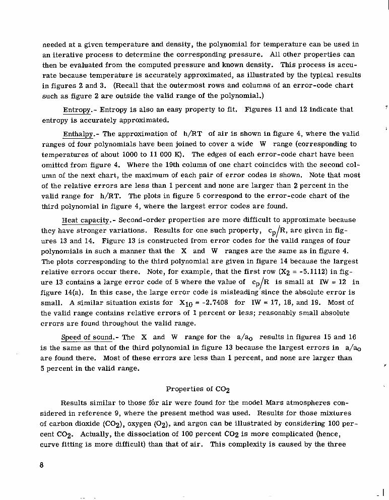
needed at a given temperature and density, the polynomial for temperature can be used in an iterative process to determine the corresponding pressure. All other properties can then be evaluated from the computed pressure and known density. This process is accu- rate because temperature is accurately approximated, as illustrated by the typical results in figures 2 and 3. (Recall that the outermost rows and columns of an error-code chart such as figure 2 a r e outside the valid range of the polynomial.)
1 Entropy.- Entropy is also an easy property to fit. Figures 11 and 12 indicate that entropy is accurately approximated.
Enthalpy.- The approximation of h/RT of air is shown in figure 4, where the valid ranges of four polynomials have been joined to cover a wide W range (corresponding to temperatures of about 1000 to 11 000 K). The edges of each error-code chart have been omitted from figure 4. Where the 19th column of one chart coincides with the second col- umn of the next chart, the maximum of each pair of e r r o r codes is shown. Note that most of the relative e r r o r s are less than 1 percent and none a r e larger than 2 percent in the valid range for h/RT. The plots in figure 5 correspond to the error-code chart of the third polynomial in figure 4, where the largest e r ro r codes a r e found.
Heat capacity. - Second-order properties are more difficult to approximate because they have stronger variations. Results for one such property, c R, a r e given in fig- ures 13 and 14. Figure 13 is constructed from e r r o r codes for the valid ranges of four polynomials in such a manner that the X and W ranges a r e the same as in figure 4. The plots corresponding to the third polynomial a r e given in figure 14 because the largest relative e r r o r s occur there. Note, for example, that the f i rs t row (X2 = -5.1112) in fig- ure 13 contains a large e r r o r code of 5 where the value of c R is small at IW = 12 in figure 14(a). In this case, the large e r r o r code is misleading since the absolute e r r o r is small. A similar situation exists for Xi0 = -2.7408 for IW = 17, 18, and 19. Most of the valid range contains relative e r r o r s of 1 percent o r less; reasonably small absolute e r r o r s a r e found throughout the valid range.
P I
p i
Speed of sound.- The X and W range for the a/% results in figures 15 and 16 is the same as that of the third polynomial in figure 13 because the largest e r r o r s in a/% a r e found there. Most of these e r r o r s a r e l e s s than 1 percent, and none a r e larger than 5 percent in the valid range. r
Properties of C02
Results similar to those f6r air were found for the model Mars atmospheres con- sidered in reference 9, where the present method was used. Results for those mixtures of carbon dioxide (COz), oxygen (02), and argon can be illustrated by considering 100 per- cent C02. Actually, the dissociation of 100 percent C02 is more complicated (hence, curve fitting is more difficult) than that of air. This complexity is caused by the three
8
major dissociation processes for C02 (2C02 - 2CO + 0 2 , 0 2 - 20, and CO - C + 0) compared with the two for air (02 - 2 0 and N2 - 2N).
Enthalpy.- Figures 17 and 18 are for h/RT of C02, which is negative at tempera- tures below about 3000 K. that the e r ro r code is meaningless where h/RT passes through zero. This problem has been avoided in the e r r o r codes of figure 17 by simply adding a constant to h/RT to pre- vent the property from passing through zero. The first polynomial approximates h/RT + 45; the second, h/RT + 15; and the last two, h/RT. The X and W ranges in figure 17 a r e the same as those for air in figure 4. The largest of the relative e r r o r s i n the valid range is 4 percent, and most of the e r r o r s a r e less than 2 percent. largest e r r o r codes occur in the third polynomial, plots for it a r e given in figure 18.
The negative values pose no problem in curve fitting except
I
L
Since the
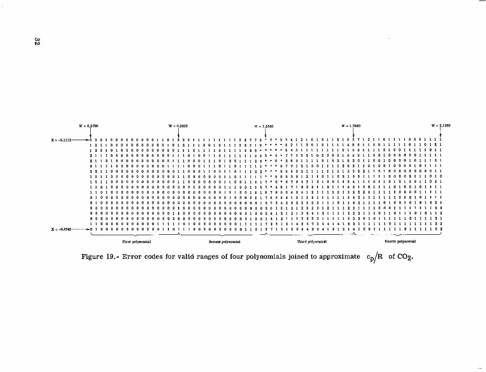
Heat capacity.- Results for c R of C02 a r e given in figures 19 and 20 for the same X and W ranges as before. In figure 19, as in previous figures, the largest e r ro r codes occur in the third polynomial, for which plots a r e given in figure 20. These plots indicate that the value of cp/R is small in a reas where the e r r o r codes a r e largest. In these areas the plots in figure 20 show that the absolute e r r o r s are reasonably small.
P I
CONCLUDING REMARKS
Ninth-degree two-dimensional polynomials can be used with a coefficient-averaging technique to approximate thermodynamic properties of air and model planetary atmo- spheres. For a temperature range of about 1000 to 11 000 K and a pressure range of 10-5 to 100 atmosphere (1 atm = 1.0133 X 10⁵ N/m2), four polynomials can be joined to approx- imate a single thermodynamic property. These four polynomials would be stored in a computer as 400 polynomial coefficients. Relative e r r o r s of less than 1 percent a r e found over most of the applicable range.
Langley Research Center, National Aeronautics and Space Administration,
Hampton, Va., June 27, 1972.
9

APPENDIX
DETERMINATION O F POLYNOMIAL COEFFICIENTS
The 400 values of any property Z, as illustrated in figure 1, are used to determine the 100 coefficients of the two-dimensional ninth-degree polynomial
::: Bo, 1
B1, l
B2, l
B9, l
_ . 1
W
N2
Y9 . -
where
and
x -x1 1 x20 -x1
W - W l - - 1
W 2 0 - h -I X =
W =
I
I \
These variables x and w are norma1,Led to range between -0.5 and 0.5 to avoid le possibility of ill-conditioning (ref. 10) in matrices whose elements are powers of x's o r w's. The normalization is also numerically convenient, since the x's and w's always have the same values: x1 = w1 = -0.5, x2 = w2 = -0.44737, x3 = w3 = -0.39474, . . ., X I 8 = w18 = 0.39474, x19 = w19 = 0.44737, and x20 = w20 = 0.5.
The solution for the 100 coefficients BmYn of equation (Al) begins by determining two "exact" one-dimensional polynomials for each given x value, with w as the vari- able. (An "exact" polynomial is referred to as a polynomial interpolating function in chapter 3 of reference 11. It passes through every point.) One polynomial is required to exactly reproduce the first, third, . . ., and the 19th property values while the other exactly reproduces the second, fourth, . . ., and 20th values. For the ith x value, one of these polynomials is found by solving
3
10

t
'1,l '1,3 '1,5 - - '1,19
'2,l '2,3 '2,5 * - zz,19
'3,l '3,3 '3,5 - * * '3,19
'4,l '4,3 '4,5 * - '4,19
'5,l '5,3 '5,5 * * '5,19
'6,l '6,3 '6,5 * . * '6,19
'20,l '20,3 '20,5 ' ' '20,1g -
- - a1,o a1,1 a1,2 . * a1,9
a2,o a2,1 a2,2 * a2,9
a3,0 a3,1 a3,2 * - a3,9
a4,0 a4,1 a4,2 * * ' a4,9
= a5,0 a5,1 a5,2 . . a5,9
a6,0 a6,1 a6,2 * a6,9
a20,o a20,1 a20,2 * * azo,!
z1,2 '1,4 '1,6 * * '1,20
'2,2 '2,4 '2,6 * '2,20
'3,2 '3,4 '3,6 * * * '3,20
'4,2 '4,4 '4,6 * * '4,20
'5,2 '5,4 '5,6 * '5,20
'6,2 '6,4 '6,6 * * . '6,ZO
=
- b1,o b l , l b1,2 - b1,9
b2,O b2 , l b2,2 * b2,9
b3,0 b3,1 b3,2 - - * b3,9
b4,0 b4,1 b4,2 . b4,9
b5,0 b5,1 b5,2 * * b5,9
b6,0 b6,1 b6,2 * - b6,9
b O , O bZ0,l b 0 , 2 . * . b o , ! -
1 1 1 . . . 1
w1 w3 w5 . . . w1g
w12 w32 w52 . . . w1g1
w19 w39 w59 . . . W19( -
1
'2
1z9
1
w4
w42
w49
1
w6
w62
w69
. . .
. . .
. . .
. . .
for the ith row of bi,n. numbered columns of figure 1; the left-hand side of equation (A4) is formed from the even- numbered columns. The two polynomials a r e then averaged to obtain one polynomial given by the ith row of equation (A5),
The left-hand side of equation (A3) is formed from the odd-
A1,o A1,l A1,2 - *
A2,o A2,l A2,2 * *
A3,0 *3,1 A3,2 - *
A4,0 A4,1 A4,2 * *
A5,0 A5,1 A5,2
A6,0 A6,1 A6,2 *
*20,0 A20,l A20,2 ' '
A1,9
A3,9
A4,9
A5,9
A2,9
A6,9
A20,!
1
W
W 2
WE . .
for i = l , 2 , . . . , 2 0 and n = 0 , 1 , . . ., %,n + bi,n where 4 n = 9 2 9.
11

APPENDIX - Continued
- _ _ - A2,O A2,l A2,2 - x2 x22 x23 . . . x29 do,0 d0,9
x4 x42 x43, . . . x49 d1,o d l , l d1,2 * d1,9
x6 XG2 x63 . . x69 d2,O d2,l d2,2 - - - d2,9
A4,0 A4,1 A4,2 *
A6,0 A6,1 A6,2 . * -
- A20,O -420,l A20,2 - - - x20 ' xZO2 xZO3 . . . x209 d g , ~ %,I d9,2 . . . d9,9 -L 4
At this point, the ith row of Zi , j is approximated by a polynomial such that
9 r-7
Z(xi,w) ), Ai,nwn n=O
for i = 1, 2, 3, . . ., 20. Now the nth column of Ai mial function of x. first solving
is to be approximated by a polyno- 1
Two "exact" polynomials are formed for the nth column of Ai,n by
A1,o A1,l A1,2 - * A1,9
A3,0 A3,1 A3,2 * - A3,9
A5,0 A5,1 *5,2 * * A5,9
'19,O A19,1 A19,2 * * A19,C
for the nth column of Cm,n and then solving
for the nth column of dm,n. numbered rows of Ai,n of equation (A5); the left-hand side of equation (A7) is formed from the even-numbered rows. The two polynomials are then averaged to obtain one polynomial given by the nth column of equation (A8),
The left-hand side of equation (A6) is formed from the odd-
12

APPENDIX - Continued
where
Cm,n + dm,n 2 Bm,n =
for m, n = 0, 1, . . ., 9. The two-dimensional polynomial approximation is finally formed by substituting Bm,n of equation (A9) into equation (Al).
u re 4 for h/RT of air are given here, and a sample evaluation of the polynomial is given. The Bm,n are ordered as follows:
The set of Bm,n and XI, X20, W1, and WzO for the third polynomial of fig-
B0,o
B0,5
B9,5
The integer following
m = 0:
m = 1:
m = 2:
m = 3:
m = 4:
m = 5:
m = 6:
m = 7:
m = 8:
m = 9:
1.88423 +O 1 2.2 529E+01
- 1.92233+01 -4.96943 +03 5.76503 -01 4.0263E+04 1.58383+01
-3.83 74E+04 -2.33103+01 -5.88253+05
1.82783+01 1.55893+06 3.19573+01 2.36223+06
1.14763+01
1.682 7E +07
-5.90663+01 -9.24743+06
-2.93863+06 -2.23173+01
B0,l B0,2 B0,3 B0,4
B9,6 B9,7 B9,8 B9,9
the E is a power of 10; for example, 1.20813+03 = 1.2081 X lo3. 1.87243+0 1 1.20813+03 5.98603+00
-8.43023+03 -7.98853+01 - 3.07 1 7E +04
1.72153+02 3.49923+05
-2.61703+02 -4.462 5E+05 -2.63753+02 - 2.3 79 1E+O 6
1.76673+03 5.30443+06
4.2 24 9E +O 6
2.19023+03 1.63 64E+06
- 1.043 7E+03
-2.643 1E+03 - 1.3 06 5E+O 7
-1.92743+01 1.80453 +03 1.47673+02 1.57513+04
7.59103+02 6.28863+05 1.88173+03 3.693 3 E +06
5.06613+03
2.95123+04 7.52633+07
1.35303+07
-4.71903+02 - 2.84 12E+O 5
-1.023 1E+04 - 1.3 535E+07
- 1.34833+07
-2.17843+04
- 2.583 8E+04 -1.34863+08
- 7.4 597E+O 1 - 2.4644E+03 4.58173+02 2.72593+04
2.8 112E+04 -1.20603+03
-3.23723+03 -9.11433+05 3.15783+04 1.7799E+06
5.7 17 5E+06 -4.67903+04
- 1.40853+05 - 1.722 1E+O 7
-7.18843+06 3.47043+0 5
1.98583+05 4.10343+07
-6.53 13E+05 -1.32483+07
- 1.4 16 1E+02 - 5.09263+03
- 1.3 0 93 E +04 1.20883+02
7.55023+03 6.098 1E+05
-3.77243+04 -1.87233+06
-7.46003+06 1.0701E+04
2.92723+05 3.42123+07
2.43993+07 -4.11313+05
- 6.6843 E+05 - 1.85083+08
-1.65643+07 1.1113E+06
2.56733+05 3.28853+08
For these values of Bm,n, the Xi , X20, W1, and W2o a r e
X i = -5.4075 Xz0 = 0.2222
W 1 = 1.3310 W20 = 1.7680
13

APPENDIX - Concluded
This polynomial for h/RT can only be used in the valid range as shown in figure 4, -5.1112 S X S -0.0741 and 1.3540 5 W S 1.7450. If, for example, h/RT is desired at the point X = -3.0 and W = 1.5, equation (A2) is used to find that x = -0.07236 and w = -0.11327. These normalized variables and Bm,n are then substituted into equa- tion (Al) to evaluate h/RT = Z(x,w) = 17.9.
?
14

RE FERENC E S
1. Barnwell, Richard W.: Inviscid Radiating Shock Layers About Spheres Traveling at Hyperbolic Speeds in Air. NASA TR R-311, 1969.
2. Grabau, Martin: A Method of Forming Continuous Empirical Equations for the Ther- modynamic Properties of Air From Ambient Temperatures to 15,000° K, With
t Applications. AGARD Rep. 333, Sept. 1959.
3. Walsh, J. L.; Ahlberg, J. H.; and Nilson, E. N.: Best Approximation Properties of i the Spline Fit. J. Math. Mech., vol. 11, no. 2, Mar. 1962, pp. 225-234.
Air From 1,500° K.to 15,000° K. Rep. No. 1921, Pratt & Whitney Aircraft, Jan. 1961.
4. Landis, F.; and Nilson, E. N.: Thermodynamic Properties of Ionized and Dissociated
5. Birkhoff, Garrett; and Garabedian, Henry L.: Smooth Surface Interpolation. J. Math. & Phys., vol. XXXM, no. 4, Dec. 1960, pp. 258-268.
6. Newman, Pe r ry A.; and Allison, Dennis 0.: Direct Calculation of Specific Heats and Related Thermodynamic Properties of Arbitrary Gas Mixtures With Tabulated Results. NASA T N D-3540, 1966.
7. Allison, Dennis 0.: Calculation of Thermodynamic Properties of Arbitrary Gas Mix- tures With Modified Vibrational-Rotational Corrections. NASA TN D-3538, 1966.
8. Guest, P. G.: Numerical Methods of Curve Fitting. Cambridge Univ. Press, 1961.
9. Allison, Dennis 0.; and Bobbitt, Percy J.: Real-Gas Effects on the Drag and Trajec- tories of a Nonlifting 140° Conical Aeroshell During Mars Entry. 1971.
NASA TN D-6240,
10. Anon.: Modern Computing Methods. Second ed., Phil. Lib., c.1961.
11. Nielsen, Kaj L.: Methods in Numerical Analysis. Second ed., Macmillan Co., c.1964.
15
I b

TABLE I.- DEFINITION O F ERROR CODES
I Error code I
0 I 1
Percent e r ro ra
0.0 to 0.1 0.1 to 1.0 1.0 to 2.0 2.0 to 3.0 3.0 to 4.0 4.0 to 5.0 5.0 to 7.0 7.0 to 10.0
10.0 to 15.0 15.0 to 20.0 20.0 to m
Z i , j - Z(xi,wj) a(Percent e r ro r ) = 100
Zi , j i , j
16

I w1 w2 w3 w4 w5 w6 - - - w20 I
x20
. . . Z Z %,20 'l,l Z 1,2 '1,3 1,4 '1,5 1,6
Z 2,l '2,2 '2,3 '2,4 '2,5 '2,6 z2,20 . . . . . .
Z Z '3,20 3,l 3,2 3,3 '3,4 3,5 3,6
'4,l '4,2 . '4,3 '4,4 Z 4,5 '4,6 '4,20
Z 5,1 '5,2 '5,3 '5,4 Z 5,5 '5,6 '5,20
Z Z '6,20
Z Z Z
. . .
. . .
. . . '6,l '6,2 Z 6,3 6,4 '6,5 6,6
. . . '20,l '20,2 '20,3 '20,4 '20,5 '20,6 z20,20
Figure 1.- Array of input values of a thermodynamic property Z.
W19 = 1.7450 wlo = Y 3 * 0 i
W2 = 1.3540
i 8 1 1 1 1 0 0 0 0 0 0 0 0 1 1 1 1 1 2 7
5 1 1 0 0 0 0 0 0 0 0 0 0 0 0 0 0 0 0 1 4 1 1 0 0 0 0 0 0 0 0 0 0 0 0 0 0 1 0 3 1 1 0 0 0 0 0 0 0 0 0 0 0 0 0 0 0 1 1 3 3 1 1 0 0 0 0 0 0 0 0 0 0 0 0 0 0 . 0 1 2 4 0 1 0 0 0 0 0 0 0 0 0 0 0 0 0 0 0 1 1
1 0 0 0 0 0 0 0 0 0 0 0 0 0 0 0 0 1 0 2 Xlo=-2.7408-1 0 0 0 0 0 0 0 0 0 0 0 0 0 0 0 0 0 1 1
1 0 0 0 0 0 0 0 0 0 0 0 0 0 0 0 0 0 0 1 1 0 0 0 0 0 0 0 0 0 0 0 0 0 0 0 0 0 0 1 1 0 0 0 0 0 0 0 0 0 0 0 0 0 0 0 0 0 0 1 0 0 0 0 0 0 0 0 0 0 0 0 0 0 0 0 0 0 0 1 0 0 0 0 0 0 0 0 0 0 0 0 0 0 0 0 0 0 0 1 0 0 0 0 0 0 0 0 0 0 0 0 0 0 0 0 0 0 0 0 1 0 0 0 0 0 0 0 0 0 0 0 0 0 0 0 0 0 0 0 0 0 0 0 0 0 0 0 0 q 0 0 0 0 0 0 0 0 0 1
X 1 g = - O . O 7 4 1 ~ 1 0 0 0 0 0 0 0 0 0 0 0 0 0 0 0 0 0 0 0
~ ~ = - 5 . i i i 2 ~ 4 1 1 o o o o o o o o a o o o o o o o 1
3 0 1 0 0 0 0 0 0 0 0 0 0 0 0 0 0 1 - 0 2
3 1 1 0 0 0 0 0 0 0 0 0 0 0 0 0 1 1 0 6
Figure 2.- Error-code chart (table I) for polynomial approximating T of air.
17

0 Input data
- Polynomial
1000
300
1100
300 I I I I I I I I I 300 I I I I I I I I
1100
0 2 11 6 8 10 12 111 16 18 20
I X
800
700
fi 600
500
0 2 4 6 8 10 12 111 16 I 8 20
IW l R 1 I X 2 [ X -5 .11121- I 0 1 I W 2 [ W 1.35901.
I I I I I I I I 0 2 9 6 8 10 12 111 16 18 PO 0 2 11 6 8 10 12 111 16 18 20
I W I X ( 8 1 IX 10 I X 7 -2.7'1081. [ E l I W 10 I W 1.53801.
1000 1000
900 900
800 800
700 x 700 x
600 fi 600
500 500
1100 1100
300 l I l l l l l l l 300 I I I I I I I I I 0 2 11 6 8 10 12 111 16 18 20 0 2 11 6 8 10 12 111 16 18 20
I W 1x [ C I I X x 13 I X -0.07911. ( F l I W 13 I W 1.79501.
Figure 3. - Comparison of polynomial approximating T of air with input data.
18

= = X = - 5 . 1 1 1 2 ~ 0 1 0 0 0 0 0 0 0 0 0 0 0 0 0 0 1 1 1 0 0 0 0 0 0 0 0 0 0 0 0 0 0 1 2 1 1 0 0 0 0 0 0 0 0 0 0 0 0 0 1 1 1 0 0 0 0 0 0 0 0 0 0 1 0 0 0 0 1
1 0 0 0 0 0 0 0 0 0 0 0 0 0 0 0 1 1 1 0 0 0 0 0 0 0 0 0 0 0 0 0 0 0 1 2 0 1 0 1 0 0 0 0 0 0 0 0 0 0 1 1 0 0 0 0 0 0 0 0 0 0 0 0 0 0 0 1 0 1 0 0 0 0 0 0 0 0 0 0 0 0 0 0 1 1 1 1 1 1 0 0 0 0 0 0 0 0 0 0 0 0 1 1 2 0 1 0 0 0 0 0 0 0 0 0 0 1 0 1 1 0 0 0 0 0 0 0 0 0 0 0 0 0 0 0 0 0 1 1 0 0 0 0 0 0 0 0 0 0 0 0 0 0 0 1 1 0 1 0 0 0 0 0 0 0 0 0 0 1 0 1 1 l 1 0 0 1 0 0 0 0 0 0 0 0 1 1 1 1 0 0 0 0 0 0 0 0 0 0 0 0 0 0 0 0 0 0 1 0 0 0 0 0 0 0 0 0 0 0 0 0 0 0 1 1 1 1 0 0 0 0 0 0 0 0 0 0 1 0 1 1 1 1 0 0 1 1 0 0 0 0 0 0 0 0 ~ 1 ~ 0 0 0 0 0 0 0 0 0 0 0 0 0 0 0 0 0 0 1 0 0 0 0 0 0 0 0 0 0 0 0 0 0 0 1 1 1 0 0 0 0 0 0 0 0 0 0 0 0 0 1 1 1 0 1 1 0 0 0 0 0 0 0 0 0 0 1 0 1 0 0 0 0 0 0 0 0 0 0 0 0 0 0 0 0 0 0 0 0 0 0 0 0 0 0 0 0 0 0 0 0 0 0 1 1 1 0 0 0 0 0 0 0 0 0 0 0 0 0 0 1 1 0 0 0 1 0 0 0 0 0 0 0 0 1 0 1 1 0 0 0 0 0 0 0 0 0 0 0 0 0 0 0 0 0
0 0 0 0 0 0 0 0 0 0 0 0 0 0 0 0 0 1 1 0 1 0 0 0 0 0 0 0 0 0 0 1 0 1 l 0 0 0 0 0 0 0 0 0 0 0 0 0 0 0 1 1 0 0 0 0 0 0 0 0 0 0 0 0 0 0 0 0 0 0 0 0 0 0 0 0 0 0 0 0 0 0 0 0 0 0 1 0 1 0 0 0 0 0 0 0 0 0 0 0 0 0 1 1 1 0 0 0 0 0 0 0 0 0 0 0 0 0 0 0 1 0 0 0 0 0 0 0 0 0 0 0 0 0 0 0 0 0 0 0 0 0 0 0 0 0 0 0 0 0 0 0 0 0 0 1 1 0 0 0 0 0 0 0 0 0 0 0 0 0 0 0 1 1 0 0 0 0 0 0 0 0 0 0 0 0 0 0 0 1 0 0 0 0 0 0 0 0 0 0 0 0 0 0 0 0 0 0 0 0 0 0 0 0 0 0 0 0 0 0 0 0 0 0 1 1 0 0 0 0 0 0 0 0 0 0 0 0 0 0 1 1 1 0 0 0 0 0 0 0 0 0 0 0 0 0 0 1 0 0 0 0 0 0 0 0 0 0 0 0 0 0 0 0 0 0 0 0 0 0 0 0 0 0 0 0 0 0 0 0 0 0 0 1 1 0 0 0 0 0 0 0 0 0 0 0 0 0 0 1 0 0 0 0 0 0 0 0 0 0 0 0 0 0 0 0 0 1 0 0 0 0 0 0 0 0 0 0 0 0 0 0 0 0 0 0 0 0 0 0 0 0 0 0 0 0 0 0 0 0 0 0 l 0 0 0 0 0 0 0 0 0 0 0 0 0 0 0 1 ~ 0 0 0 0 0 0 0 0 0 0 0 0 0 0 0 0 0 0 0 0 0 0 0 0 0 0 0 0 0 0 0 0 0 0 0 0 0 0 0 0 0 0 0 0 0 0 0 0 0 0 0 1 0 0 0 0 0 0 0 0 0 0 0 0 0 0 0 0 1 0 0 0 0 0 0 0 0 0 0 0 0 0 0 0 0 0 0 0 0 0 0 0 0 0 0 0 0 0 0 0 0 0 0 0 0 0 0 0 0 0 0 0 0 0 0 0 0 0 0 0 1 1 0 0 0 0 0 0 0 0 0 0 0 0 0 0 0 0 0 0 0 0 0 0 0 0 0 0 0 0 0 0 0 0 0 0 0 0 0 0 0 0 0 0 0 0 0 0 0 0 0 0 0 0 0 0 0 0 0 0 0 0 0 0 0 0 0 0 0 1 1 1 0 0 0 0 0 0 0 0 0 0 0 0 0 0 0 0 0 0 0 0 0 0 0 0 0 0 0 0 0 0 1 0 0 0 0 0 0 0 0 0 0 0 0 0 0 0 0 0 0
L A A A J
0 0 0 0 0 0 0 0 0 0 0 0 0 0 0 0 0 1 1 0 1 0 0 0 0 0 0 0 0 0 0 0 0 1 1 1 0 1 0 0 0 0 0 0 0 0 0 0.0 0 1 1 0 0 0 0 0 0 0 0 0 0 0 0 0 0 0 0 0
X ~ - 0 . 0 1 4 1 ~ 0 0 0 0 0 0 0 0 0 0 0 0 0 0 0 0 0 1 0 0 0 0 0 0 0 0 0 0 0 0 ~ 0 0 0 0 1 0 0 0 0 0 0 0 0 0 0 0 0 0 0 0 1 0 0 0 0 0 0 0 0 0 0 0 0 0 0 0 0 0 u v Y "
First polynomial Second polynomial Third polynomial Fourth polynomial
Figure 4.- Error codes for valid ranges of four polynomials joined to approximate h/RT of air.

1 1 L I I I I I I I I I 0 2 11 6 8 10 12 111 16 18 PO
I W ( 0 1 I X 1 2 I X I -5 .1112) .
I I I I I I I I I 0 2 'I 6 8 10 12 14 16 18 20
I N I 8 1 I X 10 ( X -2-7t I083.
211 I'
1 1 L I I I I I I I I I 0 2 11 6 8 10 12 111 16 18 20
I W I C 1 I X I 19 I X z -0.07Lill.
0 Input d a t a
- Polynomial c 20
1 1 L l I I I I I I I I 0 2 11 6 8 10 12 111 16 18 20
I X I O 1 I W = 2 ( W z 1.35LfOI.
- I I I I I I I I I 0 2 11 6 8 1 0 ' 1 2 111 16 18 20
I X [ E l I W r 10 I W 1.53801.
3 2 r
Y L I I I I I I I I I 0 2 'I 6 8 10 12 111 16 18 20
I X IF1 I W 13 I W 1.7Lf501.
Figure 5.- Comparison of third polynomial of figure 4 approximating h/RT of air with input data.
20

y=31- = 3.r = X = - 5 . 1 1 1 2 ~ 0 0 0 0 0 0 0 0 0 0 0 0 0 0 0 0 0 2 2 1 1 1 0 1 1 1 1 0 1 1 0 1 0 1 6 2 2 1 1 1 1 0 1 1 1 1 1 1 1 1 1 3 4 1 1 1 1 1 0 1 1 0 1 1 1 1 1 2 2
0 0 0 0 0 0 0 0 0 0 0 0 ~ 0 0 0 0 0 2 3 1 1 0 1 0 1 0 1 1 0 1 1 0 1 0 4 4 2 1 1 1 1 1 0 1 1 1 1 0 1 1 2 6 2 2 0 1 1 1 1 0 1 1 0 1 1 1 1 3 2 0 0 0 0 0 0 0 0 0 0 0 0 0 0 0 0 0 5 2 1 0 1 0 0 0 0 0 0 0 0 0 1 1 1 1 2 2 1 1 1 0 0 0 0 0 0 1 0 1 0 2 2 3 0 1 0 1 0 0 0 0 0 0 1 0 1 0 2 0 0 0 0 0 0 0 0 0 0 0 0 0 0 0 0 0 0 3 4 1 1 1 1 1 0 0 0 0 0 0 0 1 1 1 ? 6 2 1 1 0 1 0 0 0 0 0 0 1 1 1 1 5 1 1 0 1 0 0 0 0 0 1 0 1 1 1 1 1 1 0 0 0 0 0 0 0 0 0 0 0 0 0 0 0 0 0 3 3 1 1 0 1 0 0 0 0 0 0 1 0 1 0 2 1 7 1 2 1 1 1 0 1 0 1 0 1 0 1 1 2 2 3 1 1 1 0 0 0 0 0 0 0 0 0 1 0 1 1 0 0 0 0 0 0 0 0 0 0 0 0 0 0 0 0 0 4 1 1 0 1 0 0 0 0 0 0 0 0 1 1 1 2 7 4 2 1 1 1 0 1 1 0 1 0 1 1 1 1 3 2 2 1 1 0 0 0 0 0 0 1 0 1 0 1 1 2 1 0 0 0 0 , 0 0 0 0 0 0 0 0 0 0 0 0 0 3 3 1 1 1 0 1 0 0 0 0 0 0 0 0 1 0 7 4 2 1 1 0 1 1 0 1 0 1 0 1 1 1 2 3 1 1 0 1 0 0 0 0 0 0 0 0 0 0 1 1 1 0 0 0 0 0 0 0 0 0 0 0 0 0 0 0 0 0 1 3 1 1 0 1 0 0 0 0 0 0 1 0 1 0 2 4 6 1 2 1 1 1 0 1 0 1 0 1 0 1 1 2 2 3 1 1 1 0 0 0 0 0 0 0 0 0 1 0 1 1 0 0 0 0 0 0 0 0 0 0 0 0 0 0 0 0 0 2 2 1 1 0 1 0 0 0 0 0 0 0 0 1 1 2 3 5 1 2 0 1 0 1 0 1 1 0 1 0 1 1 3 1 2 0 1 0 1 0 1 0 0 0 0 0 0 1 0 2 1 0 0 0 0 0 0 0 0 0 0 0 0 0 0 0 0 0 2 1 1 1 1 0 0 0 0 0 0 0 0 0 0 1 1 5 1 1 0 1 1 1 1 0 1 0 1 0 1 1 1 2 2 1 1 0 1 0 0 0 0 0 0 0 0 0 0 1 1 1 0 0 0 0 0 0 0 0 0 0 0 0 0 0 0 0 0 1 2 1 1 0 1 0 0 0 0 0 0 0 0 1 1 1 4 4 1 1 1 1 1 1 1 0 0 0 0 1 1 1 1 2 2 1 1 1 1 0 0 0 0 0 0 0 0 0 0 1 1 0 0 0 0 0 0 0 0 0 0 0 0 0 0 0 0 0 1 1 0 1 0 0 0 0 0 0 0 0 0 0 1 0 1 1 4 0 1 0 1 0 1 0 0 0 0 1 0 1 0 2 1 1 0 1 0 1 0 0 0 0 0 0 0 0 1 0 1 1 0 0 0 0 0 0 0 0 0 0 0 0 0 0 0 0 0 1 1 0 0 0 0 0 0 0 0 0 0 0 0 0 1 1 2 1 1 0 1 0 0 0 0 0 0 0 0 1 1 1 2 2 1 1 1 1 1 0 1 0 ~ 0 0 0 0 0 0 1 1 1 0 0 0 0 0 0 0 0 0 0 0 0 0 0 0 0 0 1 1 0 0 0 0 0 0 0 0 0 0 0 0 0 0 1 1 2 1 1 0 1 0 0 0 0 0 0 0 1 0 1 1 2 1 0 1 0 1 0 0 0 0 0 0 0 0 1 0 1 1 0 0 0 0 0 0 0 0 0 0 0 0 0 0 0 0 0 0 1 0 0 0 0 0 0 0 0 0 0 0 0 0 1 1 2 1 1 1 1 1 0 1 1 1 1 0 1 1 1 1 1 1 2 1 1 1 1 0 1 1 1 1 1 1 1 0 1 1 1 0 0 0 0 0 0 0 0 0 0 0 0 0 0 0 0 0 1 1 0 0 0 0 0 0 0 0 0 0 0 0 1 0 1 1 2 0 1 0 1 1 1 1 0 1 1 0 1 1 1 1 2 1 0 1 0 1 1 0 1 1 0 1 1 1 1 0 1 1 0 0 0 0 0 0 0 0 0 0 0 0 0 0 0 0 0 0 3 0 1 0 1 1 1 1 0 1 1 0 1 1 1 1 6 ? 2 2 1 2 1 2 1 1 2 1 1 1 1 2 3 4 6 2 2 1 2 1 2 2 1 2 2 1 2 1 2 1 4
X ~ - 0 . 0 ? 4 1 ~ 0 0 0 0 0 0 0 0 0 0 0 0 0 0 0 0 0 2 1 1 1 1 1 1 0 1 1 0 1 1 1 1 0 2 4 7 1 2 1 1 1 1 2 1 1 2 1 2 2 1 4 4 5 1 2 1 1 1 1 2 2 1 2 ~ 1 3 1 ~ 1 - A A A I - First polynomial
- Second polynomial
- Third polynomial
- Fourth polynomial
Figure 6.- Error codes for valid X and Y ranges of four polynomials joined to approximate h/RT of air.

W = 2.1360 W = 1.7450 =
I I I I V
W = 0.5120 W = 0.9630
X = - 5 . 1 1 1 2 ~ 1 1 0 1 0 0 0 0 0 0 1 0 1 1 1 1 O 1 0 0 O O 0 1 0 1 2 2 1 1 0 1 1 0 1 0 0 1 0 1 0 0 0 0 0 1 0 1 0 1 0 1 1 0 1 0 1 0 0 0 0 0 1 1 0 1 1 2 0 1 1 0 0 0 0 0 1 1 0 1 2 1 1 1 1 1 0 1 0 1 0 1 1 0 0 0 0 0 0 0 1 0 1 0 0 1 1 1 0 0 0 0 0 0 0 0 0 0 1 2 1 1 1 0 0 0 0 1 0 1 0 1 1 1 1 1 1 1 0 1 1 0 1 0 2 1 0 0 0 0 0 0 0 0 0 0 1 0 0 1 0 0 0 0 0 0 0 0 0 0 1 1 2 1 1 0 0 0 0 0 0 0 0 0 1 2 1 1 1 0 0 0 1 0 1 1 1 1 1 0 0 0 0 0 0 0 0 0 0 1 0 0 1 0 0 0 0 0 0 0 0 0 0 0 0 1 1 1 0 1 0 0 0 0 0 0 0 0 1 1 1 1 1 1 0 0 0 0 0 1 1 1 0 0 0 0 0 0 0 0 ~ 0 0 0 0 0 1 0 0 0 0 0 0 0 0 0 0 0 1 1 0 1 0 1 0 0 0 0 0 0 1 1 1 1 0 0 0 0 0 0 0 1 1 1 1 0 0 0 0 0 0 0 0 0 0 0 0 0 0 1 0 0 0 0 0 0 0 0 0 0 0 1 1 1 1 0 0 0 0 0 0 0 0 1 1 1 0 1 0 1 1 0 0 0 1 0 1 1 0 0 0 0 0 0 0 0 0 0 0 0 0 0 0 0 0 0 0 0 0 0 0 0 0 0 1 1 1 1 0 0 0 0 0 0 0 0 0 1 1 0 0 0 0 0 0 0 0 0 1 1 1 0 0 0 0 0 0 0 0 0 0 0 0 0 0 0 0 0 0 0 0 0 0 0 0 0 0 1 1 1 1 1 0 0 0 0 0 0 0 1 1 0 0 0 0 0 0 0 0 0 0 1 1 1 0 0 0 0 0 0 0 0 0 0 0 0 0 0 0 0 0 0 0 0 0 0 0 0 0 0 0 1 0 1 0 0 0 0 0 0 1 0 1 0 1 0 0 0 0 0 0 0 0 0 0 0 1 0 0 0 0 0 0 0 0 0 0 0 0 0 0 0 0 0 0 0 0 0 0 0 0 0 0 1 0 0 0 0 0 0 0 0 0 0 0 1 1 0 0 0 0 0 0 0 0 0 0 0 1 0 0 0 0 0 0 0 0 0 0 0 0 0 0 0 0 0 0 0 0 0 0 0 0 0 0 0 1 1 0 0 0 0 0 0 0 0 0 0 0 1 0 0 0 0 0 0 0 0 0 0 0 0 1 0 0 0 0 0 0 0 0 0 0 0 0 0 0 0 0 0 0 0 0 0 0 0 0 0 0 1 0 0 0 0 0 0 0 0 0 0 0 1 0 1 0 0 0 1 0 0 1 0 0 0 1 1 0 0 0 0 0 0 0 0 0 0 0 0 0
Xs-0.0741-0 0 0 0 0 0 0 0 0 0 0 0 0 1 0 0 0 0 0 0 0 0 0 0 0 0 0 1 0 ' 0 0 0 0 0 0 0 0 0 0 1 1 0 0 0 0 0 0 0 0 0 0 0 0 \ A A A J - 4 " v
Second polynomial Third polynomial Fourth'polynomial First polynomial
Figure 7.- Erro r codes for valid ranges of four seventh-degree polynomials joined to approximate h/RT of air.

w2 = O T 3 0 w19 i 1*3540
0 2 0 1 0 0 0 0 0 0 0 0 0 0 0 1 0 1 0 7
0 3 0 1 0 1 0 0 0 0 0 0 0 0 0 0 0 0 0 2 0 2 0 1 0 1 0 0 0 0 0 0 0 0 0 0 0 1 1 3 0 1 0 0 0 1 0 0 0 0 0 0 0 1 0 1 0 1 0 7
0 2 0 1 0 1 0 0 0 0 0 0 0 0 0 0 0 1 0 7 0 2 0 1 0 1 0 0 0 0 0 0 0 0 0 0 0 0 0 1 0 1 0 1 0 1 0 0 0 0 0 0 0 0 0 1 0 1 0 6 0 1 0 0 0 0 0 0 0 0 0 0 0 0 0 1 0 1 0 7 0 2 0 1 0 0 0 0 0 0 0 0 0 0 0 1 0 1 0 7 0 1 0 1 0 0 0 0 0 0 0 0 0 0 0 0 0 1 0 3 0 1 0 1 0 . 0 0 0 0 0 0 0 0 0 0 0 0 1 0 4
0 1 0 0 0 0 0 0 0 0 0 0 0 0 0 0 0 1 0 5 0 1 0 1 0 0 0 0 0 0 0 0 0 0 0 0 0 0 0 1 0 1 0 0 0 0 0 0 0 0 0 0 0 0 0 0 0 0 0 2 1 1 0 1 1 0 0 0 0 0 1 0 0 0 0 0 0 1 0 2
3 3 2 4 3 1 2 2 0 2 2 1 1 1 0 1 1 4 1 *
X --5.1112-1 2 1 1 0 0 0 0 1 0 0 0 0 0 0 0 0 1 0 3 2 -
0 2 0 1 0 0 0 0 0 0 0 0 0 0 0 1 0 1 0 8
0 0 0 0 0 0 0 0 0 0 0 0 0 0 0 0 0 1 0 6
Xl9=-O.0741-O 0 0 0 0 0 0 0 0 0 0 0 0 0 0 0 0 0 0 2
Figure 8. - Error-code chart for polynomial without averaging approximating h/RT of air in same range as second polynomial of figure 4.
W20 = 2.2970 W1 = 0.5490
X1=-6.2964-* J. * * 5 * 3 7 3 3 1 5 6 6 4 1 5 2 8 4 1 * * * * * * 1 6 2 3 2 4 3 4 6 1 6 1 9 1 * * * * * 9 2 5 1 2 3 3 1 5 5 2 6 1 9 3 * * * * * 8 ' 2 3 1 1 2 2 2 5 4 3 6 3 9 6 * * * 9 * 6 4 2 1 1 2 1 3 5 3 4 5 4 8 8 *
* * * * 1 6 2 1 1 2 1 3 4 1 4 4 5 8 8 * * * * * 7 6 1 1 2 1 2 3 3 2 4 2 6 7 9 * * * * * 8 7 0 2 1 1 2 3 1 3 4 1 5 4 9 * * * * * 9 7 1 2 1 0 2 2 1 4 3 3 5 2 8 1 * * * * * 7 3 3 1 0 2 1 2 4 2 4 4 6 8 * * * * 8 * 6 4 3 0 1 1 0 2 4 1 5 2 7 7 * * 7 * 6 * 5 5 3 1 1 1 1 2 2 2 6 1 8 4 * * 8 * 0 9 3 5 ' 3 1 2 0 1 2 1 3 5 2 8 1 * * * * 5 8 1 5 2 2 2 1 0 1 1 3 4 3 8 5 *
* * 7 7 4 3 3 1 2 2 1 1 1 1 1 1 4 6 7 * * * 6 7 1 3 2 1 2 1 1 1 0 0 0 1 3 4 7 * * * 9 6 3 3 1 2 1 1 1 1 1 1 1 1 2 1 7 * * 9 9 5 4 2 1 1 1 1 1 1 1 1 1 0 1 1 4 6
X20=2.1482-* 7 * 4 6 4 1 1 2 4 7 7 2 4 3 3 6 6 9 *
* * * 7 7 2 4 1 2 2 0 1 0 1 2 2 4 7 7 *
Figure 9.- Error-code chart for polynomial approximating h/RT of air over very wide X and W range.
23

W2 = 1.3540 I
W19 = 1.7450 I 8 ~ 1 1 1 0 1 0 0 1 1 1 1 0 0 1 1 1 0 2
X2=-3.0371-7 0 1 0 1 0 0 0 0 0 0 0 0 0 0 0 0 1 0 6 1 1 0 0 0 0 0 0 0 0 0 0 0 0 0 0 0 1 1 6 3 1 1 0 0 0 0 0 0 0 0 0 0 0 0 0 0 0 1 2 4 0 1 0 0 0 0 0 0 0 0 0 0 0 0 0 0 1 1 1 3 0 1 0 0 0 0 0 0 0 0 0 0 0 0 0 0 1 0 2 1 0 0 0 0 0 0 0 0 0 0 0 0 0 0 0 0 0 0 2 0 0 0 0 0 0 0 0 0 0 0 0 0 0 0 0 0 0 0 1 1 0 0 0 0 0 0 0 0 0 0 0 0 0 0 0 0 0 0 1 1 0 0 0 0 0 0 0 0 0 0 0 0 0 0 0 0 0 0 0 1 0 0 0 0 0 0 0 0 0 0 0 0 0 0 0 0 0 0 0 1 0 0 0 0 0 0 0 0 0 0 0 0 0 0 0 0 0 0 0 0 0 0 0 0 0 0 0 0 0 0 0 0 0 0 0 0 0 0 0 0 0 0 0 0 0 0 0 0 0 0 0 0 0 0 0 0 0 0 0 0 0 0 0 0 0 0 0 0 0 0 0 0 0 0 0 0 0 0 0 0 0 0 0 0 0 0 0 0 0 0 0 0 0 0 0 0 0 0 0 0 0 0 0 0 0 0 0 0 0 0 0 0 0 0 0 0 0 0 0 1 0 0 0 0 0 0 0 0 0 0 0 0 0 0 0 0 0 0 1
0 0 0 0 0 0 0 0 0 0 0 0 0 0 0 0 0 0 1 6 0 1 1 1 0 0 0 0 0 1 1 1 1 1 1 1 1 1 7
x19=2.0000-1
Figure 10.- Error-code chart for polynomial approximating h/RT of air in same W range as that of third polyno- mial of figure 4 but in a higher X range.
W2 = 1.3540 Wl0 = 1.5380
I W19 = 1.7450
I t I t
5 1 1 0 0 0 0 0 0 0 0 0 0 1 1 1 1 1 1 4 X2=-5.1112-3 1 1 0 0 0 0 0 0 0 0 0 0 0 0 0 0 0 0 1
4 1 1 0 0 0 0 0 0 0 0 0 0 0 0 0 0 0 0 1 3 0 1 0 0 0 0 0 0 0 0 0 0 0 0 0 0 1 0 2 1 1 0 0 0 0 0 0 0 0 0 0 0 0 0 0 0 1 0 3 1 1 0 0 0 0 0 0 0 0 0 0 0 0 0 0 0 0 1 2 2 0 1 0 0 0 0 0 0 0 0 0 0 0 0 0 0 0 1 1 2 0 0 0 0 0 0 0 0 0 0 0 0 0 0 0 0 0 0 1 1 0 0 0 0 0 0 0 0 0 0 0 0 0 0 0 0 0 0 2
X l o = - 2 . 7 4 0 8 F 0 0 0 0 0 0 0 0 0 0 0 0 0 0 0 0 0 0 0 1
1 0 0 0 0 0 0 0 0 0 0 0 0 0 0 0 0 0 0 1 1 0 0 0 0 0 0 0 0 0 0 0 0 0 0 0 0 0 0 1 0 0 0 0 0 0 0 0 0 0 0 0 0 0 0 0 0 0 0 1 0 0 0 0 0 0 0 0 0 0 0 0 0 0 0 0 0 0 0 0 0 0 0 0 0 0 0 0 0 0 0 0 0 0 0 0 0 0 0 0 0 0 0 0 0 0 0 0 0 0 0 0 0 0 0 0 0 0 0 0 1 0 0 0 0 0 0 0 0 0 0 0 0 0 0 0 0 0 0 1
Xl9=-O.0741-1 0 0 0 0 0 0 0 0 0 0 0 0 0 0 0 0 0 0 0 4 1 1 0 0 0 0 0 0 0 0 0 0 0 0 0 0 1 0 6
1 0 0 0 0 0 0 0 0 0 0 0 0 0 0 0 0 0 0 1
Figure 11.- Error-code chart for polynomial approximating s/R of air.
24

92
8Y
76
68 E \ 0
60-
52
99
92-
89 - o Input data
- 76 - - Polynomial -
68 - - cc \ 0
60 - 0
52 - -
99 - -
3 6 1 1 1 3 6 . 1 1 I I I I I
36L 0 2 I 9 I 6 I A Ib 1; I \ 16 -0 361 0 2 I Lt 1 6 I A lb I \ I \ 1 6 -0
. I W I X ( C 1 I X z 19 ( X = -0.07Lt l ) . I F ) I W = 19 [ W 1.7Y50).
Figure 12.- Comparison of polynomial approximating s/R of air with input data.
0 2 '4 6 A lb I \ I \ 16 -0
25
76
68 [r. \ 0
60
52
99
-
52
Lt'f -I -
-
-
-
3 6 1 1 1

= Oro = T 4 0 = To = reo W = 0.5720 I 1
X = - 5 . 1 1 1 2 ~ 1 5 0 2 0 1 0 1 0 1 0 1 0 1 0 1 0 3 5 1 4 5 4 1 1 1 0 1 0 0 1 1 1 1 4 3 1 1 0 1 2 1 3 2 5 1 2 1 1 2 1 4 1 0 1 0 1 1 0 1 0 1 0 1 1 1 1 1 6 3 3 1 1 1 1 0 1 0 1 0 1 0 1 1 1 2 1 3 1 2 2 3 3 1 1 1 1 1 1 1 1 0 2 2 6 1 2 1 1 1 1 2 2 3 1 3 0 2 1 4 3 1 1 0 0 1 1 0 1 1 1 0 1 1 1 1 2 1 3 1 1 0 1 0 0 0 0 0 0 0 0 1 0 1 1 2 3 1 1 2 2 1 1 1 1 0 1 0 1 1 0 1 2 4 1 1 1 1 1 1 1 2 2 2 4 1 5 1 7 1 0 0 0 0 1 1 1 1 1 0 1 0 1 1 1 0 2 2 2 1 1 1 0 0 0 0 0 0 0 0 0 0 1 1 6 2 2 2 1 2 0 0 1 1 0 0 0 0 0 1 1 4 2 1 1 0 1 1 1 1 1 1 3 3 3 5 3 ~ 6 1 0 0 0 1 1 1 0 1 1 0 0 1 1 1 1 1 2 2 1 1 0 1 0 0 0 0 0 0 1 0 0 0 1 6 3 2 1 2 1 1 1 0 1 0 0 0 0 0 0 0 3 2 1 1 1 1 1 1 1 0 1 2 1 4 2 4 5 7 1 1 0 0 1 1 1 0 1 1 0 1 0 1 1 1 1 1 2 1 1 0 1 0 0 0 0 0 0 1 0 1 0 1 6 5 2 2 1 1 1 1 1 1 1 1 1 1 1 1 1 2 3 1 1 1 1 1 1 1 1 1 1 3 2 3 3 4 7 1 1 1 0 0 1 1 1 0 1 1 0 1 0 1 0 0 1 2 0 1 0 0 0 0 0 0 0 0 0 0 1 0 1 2 6 1 2 1 1 1 1 1 0 1 0 1 0 1 1 2 1 3 1 1 1 1 1 1 1 1 1 1 2 1 5 1 7 3 0 0 0 1 1 1 1 1 1 0 1 1 0 1 0 1 0 0 1 0 1 0 0 0 0 0 0 0 0 0 0 0 0 1 5 5 1 2 1 1 1 1 1 1 1 1 1 1 1 1 3 2 2 0 0 1 1 1 1 1 1 1 1 1 2 4 3 ~ 5 1 0 0 0 1 1 1 1 1 0 0 1 0 0 1 1 0
X = - 2 . 7 4 0 8 ~ 0 1 0 0 0 0 0 0 0 0 0 0 0 0 0 0 1 7 0 2 1 1 1 1 1 1 1 1 1 1 1 1 1 3 2 1 1 1 1 1 0 1 1 1 1 1 0 1 1 4 6 7 1 0 0 0 0 0 1 1 1 1 0 0 0 0 0 1 1 0 1 0 0 0 0 0 0 0 0 0 0 0 0 0 0 1 6 4 2 1 1 1 1 0 1 1 1 1 1 1 0 1 1 2 1 0 1 1 1 0 0 1 1 1 1 1 1 1 2 1 1 0 0 0 0 0 0 0 0 1 1 1 0 0 0 0 0 1 0 0 0 0 0 0 0 0 0 0 0 0 0 0 0 0 1 4 6 1 1 1 1 1 0 1 0 1 0 1 1 1 1 2 2 1 1 0 1 1 1 0 1 1 1 1 1 1 2 0 5 3 1 0 0 0 0 0 0 0 0 0 1 1 0 0 0 0 0 0 0 0 0 0 0 0 0 0 0 0 0 0 0 0 0 0 2 5 0 1 0 1 1 1 1 1 1 1 1 1 2 1 4 1 1 0 1 1 1 1 0 0 1 1 1 1 1 1 1 4 3 0 0 0 0 0 0 0 0 0 0 0 0 1 0 0 0 0 0 0 0 0 0 0 0 0 0 0 0 0 0 0 0 0 1 5 1 1 1 1 1 1 1 1 1 1 1 1 1 2 1 4 3 1 0 0 1 1 1 0 0 0 1 1 1 0 1 1 2 4 1 0 0 0 0 0 0 0 0 0 0 0 0 0 0 0 1 0 0 0 0 0 0 0 0 0 0 0 0 0 0 0 0 0 5 3 1 1 1 0 1 1 0 1 0 1 0 1 1 1 1 3 1 0 0 0 1 1 1 0 0 0 1 1 1 1 1 0 2 1 0 0 0 0 0 0 0 0 0 0 0 0 0 0 0 0
0 0 0 0 0 0 0 0 0 0 0 0 0 0 0 0 0 1 2 1 1 0 1 0 0 1 1 0 1 1 1 1 1 2 1 1 0 1 0 0 1 1 1 0 0 0 0 0 0 1 0 1 1 0 0 0 0 0 0 0 0 0 1 0 0 0 0 1 0 0 1 0 0 0 0 0 0 0 0 0 0 0 1 0 1 2 3 7 1 3 2 1 1 1 1 0 1 1 0 0 1 2 2 3 4 1 1 0 1 0 0 1 1 1 1 0 1 1 1 3 2 3 1 1 1 0 1 1 0 1 1 1 1 1 0 1 0 2
X = - 0 . 0 7 4 1 ~ 0 0 0 0 0 0 0 0 0 0 0 0 0 0 0 1 ? 4 4 2 1 1 1 1 1 1 1 1 1 0 1 1 2 5 1 1 1 1 1 0 1 0 0 0 0 1 0 0 1 0 1 3 1 1 0 1 0 0 0 1 1 1 1 1 0 1 1 1 0 L A A A J
0 0 0 0 0 0 0 0 0 0 0 0 0 0 0 1 1 3 3 1 0 1 1 0 0 1 0 1 0 1 1 1 1 2 1 1 0 0 0 0 1 1 1 0 0 1 1 1 0 1 1 , 1 1 0 1 0 . 0 0 0 0 0 1 0 0 1 0 0 0 1
v v v " Fourth polynomial First polynomial Second polynomial Third polynomial
Figure 13.- Er ror codes for valid ranges of four polynomials joined to approximate c R of air. P I

IYO- 1110-
120
100
(I --. LL
60-
Y O
20 20 -
O I I I I I I 1 I I . I 0 2 9 6 8 10 12 111 16 18 20
- 0 I npu t data
- Polynomial -
-
-
0 l l l l l l l l ~ 0 2 Y 6 8 10 I2 111 16 18 20
Figure 14.- Comparison of third polynomial of figure 13 approximating cp/R of air with input data.
IYO-
120-
100-
80 K \ LL
60-
110
20
27
1110-
120-
100-
80 - K \ LL
-
60-
- YO -
- 20 -
0 l l l l l l l l ~ O I I I I I I I I I - A 0 2 Y 6 8 IO 12 111 16 18 20 0 2 11 6 8 IO 12 111 16 18 20
1110-
120
100-
\ LL
60-
Y O -
20
! Y o -
- 120-
100- O
80 - \ LL
60-
Y O -
- 20 -
O I I I I I I I I I I 0 l l l l l l l l ~ 0 2 '1 6 8 IO 12 111 16 18 20 0 2 Y 6 8 10 12 111 16 18 20

W2 = 1.3540 Wl0 = 1.5380 W19 = 1.7450
1 1 1 * 2 6 1 2 1 1 0 1 0 1 1 0 3 4 2 4 2 8 *
X 2 = - 5 . 1 1 1 2 u * 5 4 1 1 1 1 1 0 1 1 0 1 0 1 1 1 2 4 * * 2 5 1 2 1 1 1 1 1 0 1 1 1 1 1 1 1 3 3 * 2 4 1 1 0 1 0 1 0 1 1 1 1 0 1 1 3 2 *
9 2 1 1 1 1 0 1 0 0 0 1 1 0 1 1 1 3 3 * * 2 2 1 1 0 1 0 1 1 0 1 0 1 1 1 1 1 3 6 * 1 2 0 1 0 1 0 0 0 1 0 0 1 0 1 1 2 2 8 8 1 1 0 1 0 0 0 0 0 0 0 1 0 1 1 1 2 0 9
X l o = - 2 . 7 4 0 8 ~ 1 1 0 0 0 0 0 0 0 0 0 0 0 0 0 0 1 1 1 8 6 1 1 0 0 0 0 0 0 0 0 0 0 0 0 0 1 0 1 4 5 0 1 0 0 0 0 0 0 0 0 0 0 0 0 1 0 1 1 2 3 0 1 0 0 0 0 0 0 0 0 0 0 0 0 0 0 1 0 4 1 0 0 0 0 0 0 0 0 0 0 0 0 0 0 0 0 0 1 2 0 0 0 0 0 0 0 0 0 0 0 0 0 0 0 0 0 0 1 1 1 0 0 0 0 0 0 0 0 0 0 0 0 0 0 0 0 0 0 2 2 0 0 0 0 0 0 0 0 0 0 0 0 0 0 0 0 0 0 1 2 1 0 0 0 0 0 0 0 0 0 0 0 0 0 1 0 1 1 6
X l 9 = - O . 0 7 4 1 ~ 5 0 1 0 0 0 0 0 0 0 0 0 0 1 0 0 0 1 1 2 * 4 3 1 1 1 1 1 1 0 0 1 2 1 2 3 1 7 2 *
9 3 2 1 1 1 1 0 0 1 1 0 1 1 1 1 1 4 1 *
Figure 15.- Error-code chart for polynomial approximating a/ao of air.
28

10- 10-
8-
0
\ = a
0 I I I I 1 1 - u 0
0 Input data
- Polynomial 8 -
6-
o o a - s s o = c 2 - e-0 Y--n O €+
2-
I I I I I I I I I I
10-
0
\ = a
I W I X [ C l I X z 13 ( X I -0.07911. [ F l IW = 13 ( W = 1.79501.
10-
8 - 8 -
6 - 6 - E ~ - o o o o o o o o o o o ~
\ 11- a 9 -
2- 2 -
0 l l l l l l l l . ~ 0 I I I ~ I I I I I I I
Figure 16.- Comparison of polynomial approximating a/ao of air with input data.
10-
0
\ a a
29
10-
8 - 8 -
I
P o : - - - ^
6 - 6- l s o u ^ " n -
0
\ a
Y - a Y -
2- 2 -
O I I I I I I I I I I 0 l l l l l 1 ~
B .w.

W 0
R
= O r o = O r o = = r0 X = - 5 . 1 1 1 2 ~ 0 0 0 0 0 0 0 0 0 0 0 0 0 0 0 0 0 1 1 1 0 0 0 0 0 0 1 1 0 0 0 0 1 1 4 1 2 1 1 1 0 1 1 1 1 0 1 1 1 0 1 1 1 0 0 0 0 0 0 0 0 0 0 0 0 0 0 0 1
0 0 0 0 0 0 0 0 0 0 0 0 0 0 0 0 0 1 1 0 0 0 0 0 0 0 0 0 a 0 0 0 0 1 3 4 1 1 1 1 0 0 1 0 0 1 1 1 0 1 0 1 1 0 0 0 0 0 0 0 a a 0 0 0 0 0 0 a 0 0 0 0 0 0 0 0 0 0 0 0 0 0 0 0 0 0 1 0 0 0 0 0 0 0 0 0 0 0 0 a 0 1 1 3 1 1 1 1 1 0 1 0 a 1 0 0 0 0 1 1 0 0 0 0 0 0 0 0 0 0 0 0 0 a a 0 0 o o o o o o o o o o o o o o o o o o 1 o o o o o o o o o o o o o o l 2 3 l l o l l l l o a l l o l l l l l o o o a a o o a o a a a o a o o o o a o o o o o o o o o o o o o o l l o o o o o o o o o o o o o o o 3 2 l l l l o o o l l o o o o l l o l a a a a o a a o a a a o a a a o
0 0 0 0 0 0 0 0 0 0 0 0 0 0 0 0 0 0 0 0 0 0 0 0 0 0 0 0 0 0 0 0 0 0 3 2 1 1 1 0 1 1 0 0 0 0 0 0 0 1 1 1 0 0 0 0 0 a a 0 0 a 0 0 0 a a a 0 0 0 0 0 0 0 0 0 0 0 0 0 0 0 0 0 0 0 0 0 0 0 0 0 0 0 0 0 0 0 0 0 0 0 2 3 1 1 1 1 1 0 1 1 0 0 0 1 0 0 1 1 1 1 0 a 0 0 a 0 0 0 0 0 0 0 0 0 a 0 0 0 0 0 0 0 0 0 0 0 0 0 0 0 0 0 0 0 0 0 0 0 0 0 0 0 0 0 0 0 0 0 0 0 3 0 1 0 1 0 1 1 0 1 1 0 0 1 1 1 1 1 0 1 0 a a a 0 0 0 a a a a 0 1 a o o o o o o o o a o o o o o o a o o o o a o o o o o o o o o o o o o z 2 l l o l o l o l a l l o l o l l l o o a o a a o o o o o o a o l o 0 0 0 0 0 0 0 0 0 0 0 0 0 0 0 0 0 0 0 0 0 0 0 0 0 0 0 0 0 0 0 0 0 0 2 0 1 0 1 0 0 0 a 0 0 0 0 1 1 1 1 1 1 1 0 0 0 0 a 0 0 0 0 0 a a 0 1 1 o o o o o o o a o o o o o o o o o o o o o o o o o o o o o o o o o o 2 2 l l l o o a o o o o o a a l l l l o l a a a o o o a a a a o o o l o o o o o o o a o o o o o o o o o o o o o o o o a o o o o a o o o o l 2 l l o l a o o o l o o l o l l l l l o o o a a a a o a o a o o l o 0 0 0 0 0 0 0 a 0 0 0 0 0 0 0 0 0 0 0 0 0 0 0 0 0 0 0 0 0 0 0 0 0 0 1 2 0 1 0 1 0 0 0 0 1 0 1 0 1 0 1 1 1 1 1 0 0 0 0 a a a 0 0 a a 0 1 . 1 o o o o o o o o o o a a o o o o o o o o o o o o o o o o o o o o o o l l o l o o a o o l o l o l l l l l l o o o a o a a o a a a a o o l l o o o o o o o o o o o o o o o o o o o o o o o o o o o o o o o o o o l o l o o a o o o o o o o o o l l l l o o o a o a o a a o o a a a a l 0 0 0 0 0 0 0 0 0 0 0 0 0 0 0 0 0 0 1 0 0 0 0 0 0 0 0 0 0 0 0 0 0 0 2 1 1 0 1 0 1 0 1 1 0 0 0 0 1 1 1 1 1 0 1 1 0 0 0 a a 0 0 0 0 a 0 1 0
X = - 0 . 0 1 4 1 ~ 0 0 0 0 0 0 0 0 0 0 0 0 0 0 0 0 0 1 0 0 0 0 0 0 0 0 0 0 0 0 0 0 0 0 0 2 0 1 0 1 0 1 0 0 0 0 0 1 1 1 1 1 0 0 0 0 0 0 1 0 0 0 0 0 0 0 0 ~ 1 L 2% 1 A J
0 0 0 0 0 0 0 0 0 0 0 0 0 0 0 0 0 1 0 0 0 0 0 0 0 0 0 0 0 0 0 0 0 0 3 0 1 1 1 1 0 1 ~ 0 0 0 1 0 1 1 0 1 1 0 0 0 0 0 0 0 0 0 0 0 0 0 0 0 0 0
v v v " First polynomial Second polynomial Third polynomial Fourth polynomial
Constant =. 45. Constant = 15. Constant = 0. Constant = 0.
Figure 17.- Error codes for valid ranges of four polynomials joined to approximate h/RT + Constant of C02.

112
3 6 1
36
30
211- c CC \
= 18-
12
01 I I I I I 1 I 1 - u 0 2 11 6 8 10 12 111 16 18 . 20
0 - 36 -
- 30 -
211 - \ = 18-
-
6-
O I I I
6 - 0
0 2 11 6 b ,b A -0
/sppp-e*44 O-
o l l l l l l l l a
I W ( R l I X 2 ( X -5.11121
36
30
211- c CC \
= 18-
12
30
-
-
-
0 2 11 6 b ,b A -0 I t 1 I I
6 - 0 /sppp-e*44 O-
o l l l l l l l l a
0
01 I I I I I I I 0 2 11 6 8 10 12 111 16 18 20
IW ( E l 1 X x 10 ( X = -2.7qOBI.
o Input data
- Polynomial
01 I 1 I I I I I 1 u 0 2 11 6 8 10 12 111 16 18 20
I X ( 0 1 I W 2 ( W 1.35Y01.
01 I I I I I I I I u 0 2 11 6 8 10 12 111 16 18 20
I X ( E l I W 10 ( W 1.53801.
Figure 18.- Comparison of third polynomial of figure 17 approximating h/RT of C02 with input data.
31
W N
w=or ,=r = = i""O X=-5.1112-02 0 1 0 0 0 0 0 0 0 0 0 1 1 0 1 2 2 0 1 1 1 1 1 1 1 1 1 2 2 7 7 8 * 7 * 9 1 4 1 2 1 0 1 0 1 1 2 1 8 3 7 1 2 1 1 0 1 1 1 1 0 0 1 1 1 1 1
1 2 1 1 0 0 0 0 0 0 0 0 0 0 0 1 0 1 2 1 1 1 0 0 1 0 1 1 1 2 2 3 1 g * * * * E 2 1 1 2 0 1 0 1 1 1 1 4 E 5 1 1 0 0 1 1 1 1 1 0 1 1 0 1 2 1 1 2 0 1 0 1 0 0 0 0 0 0 0 0 0 0 0 1 1 1 0 1 1 1 1 0 1 1 1 1 2 2 3 * * * * * E 4 3 1 1 1 1 1 1 1 1 2 1 6 2 1 1 1 1 0 1 0 0 1 1 1 1 1 0 1 1 2 1 1 1 0 0 0 0 0 0 0 0 0 0 0 0 1 1 1 0 1 0 0 1 1 0 1 1 1 1 1 1 3 E 9 * 5 * 7 7 3 2 2 1 0 0 0 0 0 1 6 3 2 1 1 0 0 1 0 0 0 0 0 0 1 1 1 1 1 2 1 1 0 1 0 0 0 0 0 0 0 0 0 0 0 1 1 1 0 0 0 1 1 1 0 1 0 0 1 1 1 2 5 * * E * 2 E 3 1 1 1 1 0 1 0 2 1 5 2 0 1 1 0 0 1 0 0 0 0 1 0 1 1 1 0 1
2 2 1 1 0 0 0 0 0 0 0 0 0 0 0 0 0 1 1 0 0 0 1 1 0 0 1 1 0 1 1 ~ 0 2 * * * 5 E 4 5 3 1 1 1 1 1 1 1 1 3 5 2 2 1 1 0 1 0 0 0 0 0 0 0 0 0 1 1 2 1 1 1 1 0 0 0 0 0 0 0 0 0 0 1 1 1 1 0 0 0 1 1 1 0 1 1 0 1 1 1 1 ~ * * * E 7 1 1 2 1 0 0 1 1 1 1 2 6 3 1 1 0 1 0 0 1 0 0 0 0 1 0 1 1 1 1
1 1 1 1 0 0 0 0 0 0 0 0 0 0 0 0 0 1 1 0 0 0 0 0 0 0 1 1 0 1 1 1 1 1 * * 9 9 E 5 6 1 2 1 1 0 1 1 0 2 1 5 3 1 1 1 1 1 0 0 0 0 0 ~ ~ ~ 0 ~ 0 1 1 1 1 0 0 0 0 0 0 0 0 0 0 0 0 0 1 1 0 0 0 0 0 0 0 1 1 0 0 1 1 1 1 1 * 6 * 6 7 6 4 3 1 2 1 0 0 1 1 3 4 1 1 1 0 1 1 0 1 0 1 0 0 ~ 1 0 2 1 1 1 0 1 0 0 0 0 0 0 0 0 0 0 0 0 0 0 0 0 0 0 0 0 0 0 1 1 1 0 0 ~ 1 0 1 * 4 E 1 7 1 6 2 2 1 1 2 1 1 1 4 3 1 0 0 1 1 1 1 0 1 0 0 1 0 1 1 1 1 1 1 0 1 0 0 0 0 0 0 0 0 0 0 0 0 0 0 0 0 0 0 0 0 0 0 1 1 1 0 0 1 1 1 E 7 6 5 5 4 3 4 1 2 1 1 1 1 2 1 5 2 2 2 1 1 1 1 1 ~ 0 0 0 0 1 ~ ~ ~ 1 0 1 0 0 0 0 0 0 0 0 0 0 0 0 0 0 0 0 0 0 0 0 0 0 0 0 0 1 0 0 0 0 1 1 1 6 5 3 4 1 3 1 3 2 1 1 1 1 1 1 3 4 2 1 1 1 1 1 1 1 0 1 0 1 0 ~ 1 ~ 1
0 0 0 0 0 0 0 0 0 0 0 0 0 0 0 0 0 1 0 0 0 0 0 0 0 0 0 0 0 0 0 0 0 0 2 6 1 3 1 3 1 2 3 2 3 1 2 1 1 1 2 3 1 1 1 ' 1 0 0 0 1 1 1 1 1 1 1 1 2 2 0 1 0 0 0 0 0 0 0 0 0 0 0 0 0 0 0 0 0 0 0 0 0 0 0 0 0 0 0 0 0 0 0 1 5 7 2 4 2 3 2 2 3 2 2 1 1 1 0 1 1 4 2 1 1 1 1 0 1 0 0 1 0 1 0 1 0 2 1
0 0 0 0 0 0 0 0 0 0 0 0 0 0 0 0 1 1 0 0 0 0 0 0 0 0 0 0 0 0 0 1 0 0 2 4 1 2 1 2 1 3 2 4 1 2 1 1 1 1 2 2 2 1 1 1 0 1 1 0 1 1 1 0 1 0 1 1 2 0 0 0 0 0 0 0 0 0 0 0 0 0 0 0 0 0 0 0 0 0 0 0 0 0 0 0 0 0 0 0 1 0 0 1 4 1 2 1 1 1 2 2 2 2 1 1 1 1 1 3 2 2 0 1 0 1 1 1 1 1 1 0 1 1 1 1 2 1 1 1 0 0 0 0 0 0 0 0 0 0 0 1 1 1 1 1 0 1 0 0 0 0 0 0 0 0 0 1 1 1 1 1 7 2 3 1 2 1 4 3 5 1 5 3 4 1 4 1 6 2 1 1 1 1 1 1 0 1 1 1 1 1 1 1 1 2 2
X = - 0 . 0 7 4 1 - - - - r 0 1 0 0 0 0 0 0 0 0 0 0 0 0 1 1 0 1 1 1 0 0 0 0 0 0 0 0 0 0 1 1 0 1 3 7 1 3 1 2 0 4 4 2 6 4 1 3 1 3 1 6 1 0 0 1 1 1 1 1 1 0 1 1 1 1 1 0 2 \ A h A A v
Firat polynomial v ~~
Second polynomial
v
Third polynomial
v
Fourth polynomial
Figure 19.- Error codes for valid ranges of four polynomials joined to approximate c R of C02. P I

225-
180
135
E 30- \ R
'15-
-95
NASA-Langley, 1972 - 33 L-8297 I 1 I
225
I80
-
- - 0 Input da ta
- Polynomial - 135-
0-
-
- 3 0 1 I l I I I - 3 0 1 I I I I 1 I I I I
33
225
180-
135-
r x 30-
LI Y S - \ [L
-Y5
-30
225 -
180 -
-
135-
CL 30- \ o_
Y5-
0 - 0-
4 5 - -
I I I 1 -30 I I I I 1 I I I I I 0' 2 '1 6 8 ,b /2 /11 -0 0 2 '4 6 8 IO I2 1'1 16 18 20
225-
180
I35
e
LL 4 5
I -30
225 -
180 - -
'15-0 30:-= 0 - -
gl;;:o;o 4 5 - - -
I I 1 - 3 0 - I I I I I I I I I I 0 2 'i 6 A lb lk /11-0 0 2 9 6 8 10 12 111 16 18 20

N A T I O N A L A E R O N A U T I C S A N D SPACE A D M I S T R A T I O N W A S H I N G T O N . D.C. 20546
__
USMAIL
POSTAGE A N D FEES PAID NATIONAL AERONAUTICS AND
SPACE ADMINISTRATION FIRST CLASS MAIL O F F I C I A L BUSINESS PENALTY FOR PRIVATE USE $300
NASA 451
If Undeliverable (Section 158 Postal Manual) Do Nor Return
"The aeronautical and space activities o f the United States shall be conducted so as t o contribute . . . t o t he expansion of human knowl- edge of phenomena i n the atmosphere and space. T h e Adnzinistration shall provide for the widest practicable and appropriate disseminatioia of inforntation concerning its aciitities and the results thereof."
, .
-NATIONAL AERONAUTICS A N D SPACE ACT OF 1958
NASA SCIENTIFIC AND TECHNICAL PUBLICATIONS
TECHNICAL REPORTS: Scientific and technical information considered important, complete, and a lasting contribution to existing knowledge:.
TECHNICAL NOTES: 1nformation.less broad in scope but nevertheless of importance as a contribution to existing knowledge.
TECHNICAL MEMORANDUMS: Information receiving limited distribution because of preliminary data, security classifica- tion, or other reasons.
TECHNICAL TRANSLATIONS: Information ._
published in a foreign language considered to merit NASA distribution in English.
SPECIAL PUBLICATIONS: Information derived from or of value to NASA activities. Publications include conference proceedings, monographs, data compilations, handbooks, sourcebooks, and special bibliographies.
TECHNOLOGY UTILIZATION PUBLICATIONS: Information on technology used by NASA that may be of particular interest in commercial and other non-aerospace applications. Publications include Tech Briefs, Technology Utilization Reports and Technology Surveys.
CONTRACTOR REPORTS: Scientific and technical information generated under a NASA contract or grant and considered an important contribution to existing knowledge.
Details on the availability of these publications may be obtained from:
SCIENTIFIC AND TECHNICAL INFORMATION'OFFICE
NATI 0 NA L AER 0 N AUT1 C S AND SPACE ADM I N ISTRATI 0 N Washington, D.C. PO546