polynomial inverse images and polynomial inequalities
TRANSCRIPT
Acta Math., 187 (2001), 139 160 @ 2001 by Institut Mittag-Leffier. All rights reserved
Polynomial inverse images and polynomial inequalities
b y
VILMOS TOTIK
Bolyai Institute Szeged, Hungary
and
University of South Florida Tampa, FL, U.S.A.
Dedicated to Ronald A. DeVore on his 60th birthday
1. I n t r o d u c t i o n
Let II " I[z denote the supremum norm on the set E. Two of the most used inequalities
for the derivatives of polynomials are the Bernstein inequality
Tt lx/T-_-~_ x2 I[ Pn [[ [_ 1,1] , xE [-1 , 11, IP'(x)l - -
and the Markoff inequality
[IP;~[[[-1,1] ~ n 2 IlPn[[[_l,1],
valid for polynomials Pn of degree at most n. In this paper we are primarily interested
in what form these inequalities take on several intervals. We shall see that the extension
to general sets involves the equilibrium measure of these sets. We shall give the precise
form of the Bernstein inequality for arbi trary compacts, and an asymptotical ly best form
of the Markoff inequality for sets consisting of finitely many intervals. Actually, in this
case we shall prove different Markoff inequalities one-one-associated with each one of the
endpoints of the system of intervals.
The proofs will heavily use sets that are obtained as the inverse images of inter-
vals under (special) polynomial mappings. We shall see that the original Bernstein and
This research was supported in part by the National Science Fundation, DMS-9801435, and by the Hungarian National Science Foundation for Research, T/022983.
140 v. TOTIK
Markoff inequalities instantly transfer to such polynomial inverse images (at least for
some special polynomials). From here we shall get the extension to more general sets
and more general polynomials by approximation. The approximation is based on the
density of polynomial inverse images in the family of compact sets, and we shall also
verify this density property.
We shall s tart with the just mentioned density property in the next section. Then
in w we shall consider the extension of the Bernstein inequality. Finally, the extension
of the Markoff inequality will be done in the last section.
2. Po lynomia l inverse images of intervals
Let T be a polynomial of degree N/> 2 with real and simple zeros Xx < X2 <... < XN. Let
YI<Y2<.. .<YN-1 be the zeros of T' . and assume that [T(Yj)[~>I, j = l , . . . , N - 1 (note
tha t T(Yj) are the local ex t rema of T). Then it is elementary (see [6, Lemma 1]) that
there exists a unique sequence of closed intervals El , ..., En such that for all l<~i<~N
we have T ( E J = [ - 1 , 1], X~EE~ and for l<~i<~N-1 the set E~nE~+I contains at most
one point. We call any such polynomial admissible, and we are interested in the inverse
image T - l ( [ - 1 , 1])=[.JN_IEi. We denote by Ti -1 that branch of T -1 that maps [ -1 , 1]
into Ei, and if v is a measure on [ -1 , 1], we set
T-~(L,)(A):=~,(T(A)) f o r A C E , , i = 1 .... ,N.
Polynomial inverse images of intervals, i.e. sets of the form T - 1 ( [ - 1 , 1]) with admis-
sible T, have many interesting properties. They are the sets that support weights for
which the recurrence coefficients of the associated orthogonal polynomials are periodic,
E or they are the sets = [-Ji=l [ai, bi] for which the Pell equation
p2 (z) - Q(z) S 2 (z) = 1 l
with Q(x) = I I ( x - a i ) ( x - b i ) , i = 1
that goes back to N.H. Abel, has polynomial solutions P and Q. They are also con-
nected with continued fractions and Toda lattices. For all these and many more inter-
esting results connected with polynomial inverse images see the papers [8]-[11], [13] by
F. Peherstorfer and the references there (see also [14]). However, the question if these
sets are dense among all sets consisting of finitely many intervals has been open. In this
section we prove this density, and in the subsequent sections we shall apply this result
to polynomial inequalities on several intervals.
P O L Y N O M I A L I N V E R S E I M A G E S A N D P O L Y N O M I A L I N E Q U A L I T I E S 141
THEOaEM 2.1. Given a system E={[ai , bi]}{= 1 of disjoint closed intervals and an s>0 , there is another system ' , , I I J 1 [a' b~]=r - l ( [ -1 ,1 ] ) for E ={[a~,b~]}~= 1 such that vai=lL ~,
some admissible polynomial T, and for each l <<.i<<.t we have
la,-a~l<<.e, Ib~-b~l<<.e.
The theorem immediately implies its strengthened form when we also prescribe if a
given a~ (or b~) is smaller or bigger than ai (or bi). In particular, it is possible to require
e.g. that ECE ' . The proof also shows that in the theorem we can select a'i=ai for all i,
and even b~ =bl. Alternatively we can fix any other br
N.I. Akhiezer [1] described polynomial inverse images of [-1, 1] consisting of two
intervals via elliptic functions. From here the validity of Theorem 2.1 follows when
l=2. However, if we use the characterization of polynomial inverse images given in
Lemma 2.2, then one can see that the two-interval case ( l=2 in Theorem 2.1) can be
obtained by simply changing continuously one endpoint of one of the intervals. When
l>2 the situation is more complex.
After having learned of Theorem 2.1, F. Peherstorfer [12] has also given a proof
using a completely different approach.
We shall need the following known characterization of polynomial inverse images of
intervals (see [2] and also [10]). Since the terminology is somewhat different from those
in the papers [2] or [10], for completeness we present a short proof.
l LEMMA 2.2. Let E=[.Ji=l[ai,bi] be the disjoint union of l intervals. Then E =
T-1([ -1 , 1]) for some admissible polynomial T if and only if each of the numbers
#2([a~, b~]) is rational, where Pz denotes the equilibrium measure of the set E.
For the concept of the equilibrium measure and of the logarithmic capacity of a
compact set see any text on logarithmic potentials, e.g. [20], [15] or [16]; but actually we
shall only use the defining properties (2.1) (2.2) below.
Proof. If E = T - I ( [ - 1 , 1]) and N is the degree of T, then (see [6, Theorem 11], [15])
# e = T - l ( # [ _ l , l l ) / N . Therefore if [ai,bi] consists of li subintervals T71([-1, 1]), then
p~([ai, bi])=li /N, and this proves the necessity of the condition.
Suppose now that each p~ ([ai, bi]) is rational, say #p. ([ai, b,]) = l i / N for some positive
integers N and li, i=1, ..., N. Consider the function
H(z) = e x p ( N f l og ( z - t ) d # E ( t ) - N l o g c a p ( E ) )
on the Riemann sphere C cut along E, where cap(E) denotes the logarithmic capacity
of E.
142 v. TOT1K
We need the following properties of equilibrium measures (see e.g. [15], [20, Theo-
rem III.12] or [16, Theorem 1.1.3 and Corollary II.3.4]):
flog [z-tl d~s(t) = log cap(E), z E (2.1)
f l o g (t) > log cap(N), ~ Z, (2.2) d#~ Z
and the left-hand side is a continuous function on the whole plane.
Using these and the form of #E([ai, bid we can infer that H(z) is a single-valued
analytic function on C \ N with modulus 1 on the cut Z. Thus, it easily follows that
1 1
is real-valued on both sides of the cut, and G(2)=G(z) is satisfied, hence the reflection
principle shows that this fimction can be continued analytically through each (ai,bi). Furthermore, H is bounded away from zero and infinity on compact subsets of the com-
plex plane, so G has a removable singularity at every ai and bi. Finally, H(z) has a pole of order N at infinity, therefore the same is true of G(z). In summary, G(z) is
an entire function with a pole of order N at infinity, hence G(z) is a polynomial of de-
gree N. Clearly, G(z) is real if z E R , and since we have IH(x)l=l on 2, and ] H ( x ) [ > l
and H(x) is real for all other x E R , it follows that - l~<G(x)~<l for xEZ , and IG(x ) ]> l
for x c R \ 2 . Thus, E = G - I ( [ - 1 , 1]), and all we have to show is that G is an admissible
polynomial. From the construction it is clear that for x C Z
G(x)=cos(argN/ log(x-t)dp~(t)) =cos(NTr f~d#~(t)),
from which it is clear that G has N zeros in E, and from the same formula the admissibility
of G also easily follows. []
Next we discuss the properties of the mapping
{al , bl, ..., al, bl} --+ {pE ([al, bl]), ..., # r ([at, bt])},
where E=UI1[ai,bi], and this is a disjoint union. This is a mapping of a subset of
R 2t to R l, so it is singular. It is singular even if we fix, say, the left endpoints (to
obtain a mapping from R l to R z), namely the image set is on a hyperplane, for the
sum of the coordinates in the image set is 1. Now we show that if we also fix hi, thereby
obtaining a mapping from R z-1 into the hyperplane mentioned before, then this mapping
is nonsingular.

POLYNOMIAL INVERSE IMAGES AND POLYNOMIAL INEQUALITIES 143
Thus, let
Y](Xl, ..., Xl-1 ) ~- [al, 51 + Xl] [J [a2, 52 -I-x2] U.. . [.J [al_l, bl_ 1 -+-Xl_l ] U [al, bl] ,
and we consider this set for (xl, ..., x l - 1 ) lying in a neighborhood U of the origin in R I-1
which is so small that in that neighborhood we have aj <bj +xj <aj+l for all l~<j <l. Let
M(Xl , . . . ,X l -1) - - - - (~ tE( . . . . . . . . z 1)([ a l , b l q - x l ] ) , ' ' ' , ~ t E ( x , ...... z_~) ( [a l_ l ,b l_ l -~ -Xl_ l ] ) ) . (2.3)
Then M: U--+R t - l , and we are going to show that M is a nonsingt~lar C'C-mapping,
hence in particular it is an open mapping. Thus, we can find arbitrarily close to the
origin points xl , ..., xl-1 so that all the numbers
#~(~1 ..... ~z-1)([aj,bj+xj]), l <~j<l,
are rational. Then, however,
~tE(x 1 ..... X,_l)([al, bl])
is also rational, for it complements the sum of the preceding numbers to 1. These facts
together with Lemma 2.2 prove Theorem 2.1.
We shall actually show that the Jacobian of M(Xl, ..., xz-1) is diagonally d o m i n a n t - -
this is enough to conclude the nonsingularity of M. It is known (see e.g. [17, Leinma 4.4.1],
cf. also [21]) that #z is of the form
dpz( t ) _ dt
1--1 l-L=1 It- jl l [1/2 ~r V[j=I [ ( t - a j ) ( t - b j )
(2.4)
log I x - t I du(t) = log I x - a I+ const, x E E, (2.5)
(for the existence and properties see e.g. [16, w or [7]). Since the balayage of (fo~ onto
E is #z , and since a fractional linear t ransformation preserves the balayage measure (see
below), these two questions are basically the same. We set R = R U { o c } , and identify
- o c with oc.
for tEE , where the numbers Tj lie in the intervals (bj, a j+l) . We shall need more precise
information on where these numbers lie, therefore we derive again this formula in a way
that also supplies this additional information. Actually, we need the same form and
information on the balayage measure of a Dirac mass (fa, a E R \ E , onto E. This measure
is defined as the unique measure ~, on E that has total mass 1 and for which

144 v. TOTIK
LEMMA 2.3. Let Z=U~=l [a i , b~], (bt, a l+i )=(bl , oc]U(--cx), a l ) , and for a E R \ E let
i(a) be that index l <. i<.l for which aE(b~,ai+l). The density of the balayage measure ~a
of the Dirac delta mass 6a onto E is given by
1 [IZl I ( a -a j ) (a -b j ) l 1/2 IPt_l(t)l 1 t E E , (2.6)
7r 1-Ill l ( t_a j ) ( t_b j ) l l /2 IPt_l(a)l I t - a l '
where the polynomial
P / - l ( t ) = I ] (t-mi)
ir
satisfies for all l <<.i<~l, i~ i (a ) the condition
L a~+I lit1 i (a_aj ) (a_bj ) l l /2 Pt- l ( t ) 1 I-Ill t ( t - a j ) ( t - b j ) l l / 2 Pt- l (a) It-a~] dt=O. (2.7)
This system of equations uniquely determines each "ri, i # i( a), and we have "tic (bi, ai+l)-
In particular, for a--+ec we get that the equilibrium measure #r~ is of the form (2.4)
with ~-1, ..., r l - t satisfying for all l <~ i<<.l-1
L ai+l r-[l-l(t
' ~ -~ ) dt=O. (2.8) I-Ill I ( t - a j ) ( t - b j ) l U 2
Note that the first numerator and second denominator in (2.7) are constant, so they
could be omit ted from the formulae. However, it may well happen that TZ equals oo, in
which case the factor (t--7-1)li(a--~-l) should be omit ted from all formulae. This difficulty
can be overcome by applying a fractional linear t ransformation as will be done in the
proof. The same remark applies if we want to speak of the balayage of 5oo, in which case
all the terms that contain a should be dropped.
(2.7) gives a linear ( ( l - 1)x ( l - 1))-system for the l - 1 free coefficients of Pz-1- This
system has a nonsingular matr ix (see below), and therefore the solution is unique. It
is clear from (2.7) that Pl-1 must have at least one zero on each (bi ,ai+l) , l ~ i ~ l ,
i~ i (a) , and then it cannot have more than one, so it has exactly one zero in each of
these intervals. It also follows that the coefficients of Pl-1 are C~~ of the
endpoints aj, bj, which, in view of the fact that the zeros of Pl-1 are separated, implies
tha t the zeros 7-i are also C~-funct ions of the endpoints aj,bj (Coo at co should be
understood in a proper sense, but we can always speak of normal C ~ after applying a
fractional linear t ransformation as is done below). Thus, altogether, the density of #E is
a C~176 of the endpoints aj, bj. By making the substi tution t = a i + ( b i - a i ) u we
can see that then each integral
L b'd#~(t) = #~([ai, b~]) i
P O L Y N O M I A L I N V E R S E I M A G E S A N D P O L Y N O M I A L I N E Q U A L I T I E S 145
is also a Coo-function of the variables aj, bj, and this verifies that the mapping M from
(2.3) is a C~176 on U.
Proof of Lemma 2.3. Consider the set E* obtained from E via a mapping x * =
1/(x-c~) , and for a measure u defined on E let u* be the image of u under the same
mapping x*=l/(x-(~), i.e. if E* is the image of a set E, then we set S ( E * ) = u ( E ) .
Since the balayage measure 5a of 5a onto E is characterized by the facts (see [16, w
and Theorem II.4.6]) that it is supported on E, it has total mass 1 and its logarithmic
potential
f log [z-tl 5a(t)
equals a constant plus log Iz-al on E, it is easy to see that u is the balayage of 5~
onto E if and only if u* is the balayage of 5a* onto E*, where a*=l/(a-a). It is
also straightforward to see that this same transformation also preserves the validity of
Lemma 2.3, i.e. the lemma is true for E and a if and only if it is true for E* and a*.
However, by an appropriate choice of a we can achieve tha t a* is bigger than any of the
endpoints of E*, hence we may assume from the outset that a>bl. In this case i(a)=l. Consider a polynomial
Pl-l(X) = x l - l ~-Cl-2xl-2-~-...-~-Co
and the system of equations
/b a~+l dt=O, (2.9) Pz-l( t ) !
I]Zl I(t_aj)(t_bj)ll/2 t - a
1<.i~1-1. Since the leading coefficient of Pz-1 is fixed to be 1, this is a system of linear
equations with matr ix
(fai+~ tj-i 1 ) 1 dt \Jb~ [I~i I(t_aj)(t_bj)[1/2 t -a ~i,j<~l-1
If this matr ix was singular, then by taking an appropriate linear combination of the rows
we would obtain a nonzero polynomial of degree at most I - 2 tha t was orthogonal to the
denominator in the previous formula on every interval (bi ,ai+l) , 1<~i<~1-1. However,
this would mean that this polynomial has at least one zero on each of these intervals,
which is not possible. Thus, the above matr ix is nonsingular, and the system (2.9) has
a unique solution. Clearly, the solution polynomial Pz-1 has one and only one zero on
every interval (bi, ai+l), 1~< i ~< l - 1, and hence we can write with some Ti E (bi, ai+l)
1 - 1
Pl- l (X)= H(X--Ti ). i=]
146 v. TOT1K
Consider the function
l H(z) = ~/1-[J=l(a-aj)(a-b3). Pl-l(Z)
~/H~=l(z_aj)(z_bj) P / - l ( a )
on the Riemann sphere cut along E, where we take that branch of the square root which
is positive for positive z. Let c~./3e [ai, bi]. There is a branch of l o g ( ( z - / 3 ) / ( z - o 0 ) that
is analytic outside [ai, bi]. Thus.
1 f z H(z) log z-__~ dz = H(a)log a - / 3 = log a - / 3 . 27ri z - a z - a a-c~ a-c~
Take here real parts. Since H(z)=~lH(x) l i for z=x+iO, xCE, we get
1 ~ IH(x)I log lx-/3l l a - ~ l ~r x - a ~ dx = log la_c----~,
and thus the function
1 f IH(x)l V((~) = - log [ a - a I + ]~ log Ix-~l dx
is constant on each interval [ai, bi]. Similarly, if (~ = bi,/3 = ai+l, then by cutting the sphere
along E�9 ai+l] we get as before
1 f~ H(z) log Z - 2 dz = H(a) log - - 27ri U[b~.a~+l] z--a z--a
a-/3 a-/3 = log - - . a - a a - a
Take again real parts, and notice that on (b~, a~+l) the function H(z) is real, and for
z=x• xE(bi, ai+l) we have
log - -
From these we obtain
z - / 3 = log Ix-/31 z - ~ ~ - ~ 4- iTr.
1 /~ IH(x)[, Ix-~31 la-/3[+ f a'+lH(x) dx=O. [ x - a l L o g ~ d x - l o g ~ Jb~ x--a
Here the last te rm is zero by the choice of the polynomial Pz-1, and we can conclude
that V(a) is constant on all of E. Furthermore,
1 /~ H(z) dz=H(a) = 1, 27ri z - a
P O L Y N O M I A L I N V E R S E I M A G E S A N D P O L Y N O M I A L I N E Q U A L I T I E S 147
so by taking real parts we obtain
1 ~ IH(x)l -~ " - ~ dx= 1.
Thus, the measure given by the density function
1 IH(x)l
Ix-af
is the balayage measure ~a, and the lemma is verified. []
When we form the balayage onto E of an arbi trary measure u with support on R
and with u (E)=0 , then the density is obtained by integrating the density in (2.6) with
respect to &,(a). It follows from the lemma that as a"..~bk, the numbers Ti=~-.i(a), iCk, converge to
some ~-~' that supply the solution of (2.7) for a=bk, and again ~:[E(b~, ag+l). In this case
lit1 I(a-aj)(a-bj)ll/2 = (l +o(1))Ck ax/~--bk (2.10) [Pl-l(a)l
with some positive Ck, where o(1) denotes a quanti ty tha t tends to zero as a'Nbk. Using these facts we can calculate the Jacobian of the mapping
M(Xl,..., Xl-1).
Since each of the sets E(xl , ..., xl-1) is just like E, it is enough to do that at the origin.
First let l<~k<~l-1, l<<.i<~l including i=l, but first let iCk, and we calculate the partial
derivative 0P~,(xl ...... ~-1) ( [a , b~ + x d ) (0, ..., 0)
Oxk (we set xz=0). Since iCk, this is the limit of the quotient
P~(o ..... o,xk,o ..... o)([a i ,b iD-P~([ai ,biD
Xk
as xk tends to 0 through positive values. For positive xk we have
E C E(0, ..., 0, xk, 0, ..., 0),
so p~ is the balayage of#~(o ..... o,xk,o ..... 0) onto E (see [16, Theorem IV.1.6 (e)]). Therefore,
the numerator of the preceding ratio is nothing else than the measure of [ai, bi] with
respect to the measure that we obtain by taking the balayage of
# ~ ( 0 .. . . . O,xk,O .. . . . O) I(bk,bk-Fxk)
148 v. TOTIK
onto E. Thus, in view of formula (2.6) and (2.10) the preceding ratio equals
( l + o (1 ) ) ~k [ b ~ [ bk+xk ax/~-L~-bk I]l<~j<~'ir l Jai Jbk T r a i l 1 1 ( t - a j ) ( t - b j ) l 1/~ i t_a I d#r.(o ..... o,~k,o ..... o)(a)dt.
Here for bk<a<bk+xk we have by (2.4)
dp~(o ..... 0,xk,0 ..... o ) ( a ) = ( 1 + o ( 1 ) ) Dk
x/bk + xk--a da
with some positive constant Dk. Therefore, the previous double integral can be writ ten
with some positive constant Ek.~ as
f bk+xk av/~_bk ( l+o(1) )Ek, i
Jbk v/bk +xk - a /01 da=zk ( l+o(1 ) )Ek , i u du
=xk( l+o(1) )Ek , i 1 .~Tr.
Thus, for k r
O#~(z 1 ...... t_~) ([ai, bi+xi])
Oxk (0, O) : 1 ..., ~TrEk,i.
However,
E #E(xl ...... z_~)([a~,bi+xi]) = 1, l<~i<~l
and therefore for the case k=i we obtain
cgp2(x~ ..... x,_l)([ak, bk+xk]) (0, 0) ~---- E 1 ..., -~ Tr Ek,i.
Oxk iCk
This already proves that the Jacobian of V(x 1, ..., xt_ 1 ) is diagonally dominant, since
the preceding sum is the kth diagonal element, but the sum of the kth row without this
diagonal element is
_ } - ~ 1 -~TrEk,i, l<~i<~l-1
i~s
which is smaller in absolute value than the absolute value of the kth diagonal element by 1 ~TrEk,l, and this is a positive number. []
POLYNOMIAL INVERSE IMAGES AND POLYNOMIAL INEQUALITIES 149
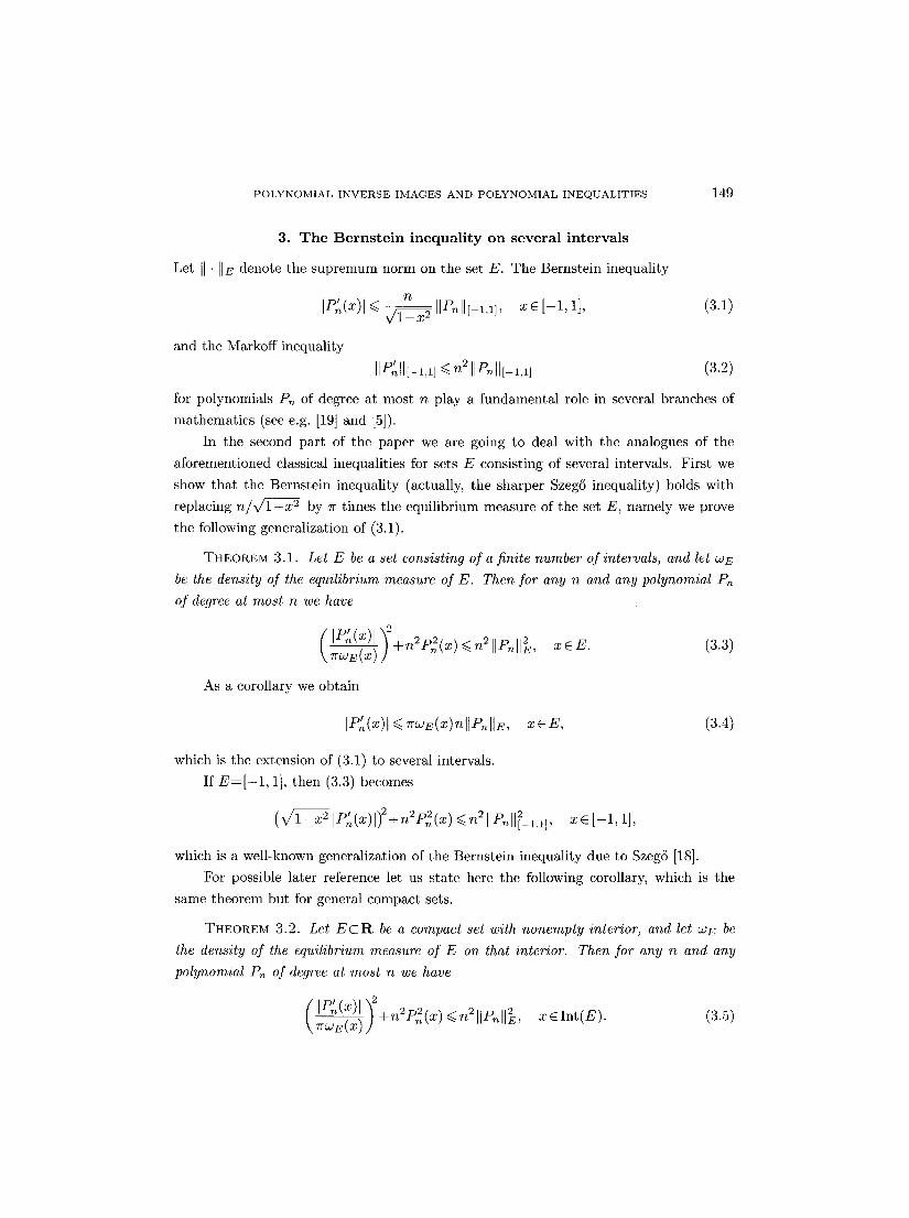
3. T h e B e r n s t e i n inequa l i ty o n severa l intervals
Let II" lIE denote the supremum norm on the set E. The Bernstein inequality
n ]Y,n/(X)] < ~ ]]PnI][-1,1], xG[-1 ,1] , (3.1)
and the Markoff inequality
IIP'II[-,,1] n 2 IIPnlI[-1,1] (3.2)
for polynomials Pn of degree at most n play a fundamental role in several branches of
mathematics (see e.g. [19] and [5]).
In the second part of the paper we are going to deal with the analogues of the
aforementioned classical inequalities for sets E consisting of several intervals. First we
show that the Bernstein inequality (actually, the sharper Szeg5 inequality) holds with
replacing n / ~ by zr times the equilibrium measure of the set E, namely we prove
the following generalization of (3.1).
THEOREM 3.1. Let E be a set consisting of a finite number of intervals, and let WE
be the density of the equilibrium measure of E. Then for any n and any polynomial Pn
of degree at most n we have
(IPrn(x)l +n2P2n(X) ~n211Pnll2E, xEE. (3.3)
As a corollary we obtain
IP'~(x)l <~ Tr~E(x)nllPnHE , x e E , (3.4)
which is the extension of (3.1) to several intervals.
If E = [ - 1 , 1], then (3.3) becomes
( l ~ X 2 ]pn/(x ) ])2+ n2pn2 (x) < n2 ]]Pn ]]~-1,1], x E [-1, 1],
which is a well-known generalization of the Bernstein inequality due to Szeg5 [18].
For possible later reference let us state here the following corollary, which is the
same theorem but for general compact sets.
THEOREM 3.2. Let E c R be a compact set with nonempty interior, and let wE be
the density of the equilibrium measure of E on that interior. Then for any n and any
polynomial pn of degree at most n we have
~'~(x)l)2+n2p2(x)<~n2 P x E Int (E) . 2 n E~ (3.5)
150 v. TOTIK
This immediately follows from Theorem 3.1. In fact, we can approximate any com-
pact set by sets E* consisting of finitely many intervals in such a manner that in the
interior of E the densities wE.(x) converge to WE(X). Since Theorem 3.1 holds with uni-
versal constant independent of the sets E*, its validity will be preserved from the sets E*
to the set E. We shall not give more details, for they are fairly standard. Of course, the
equilibrium measure PE is absolutely continuous in the interior of E, so WE is meaningful
there.
As an immediate corollary we obtain (3.4) for an arbi t rary compact set E and for
x E I n t ( E ) . Next we show that (3.4) is sharp for any compact E:
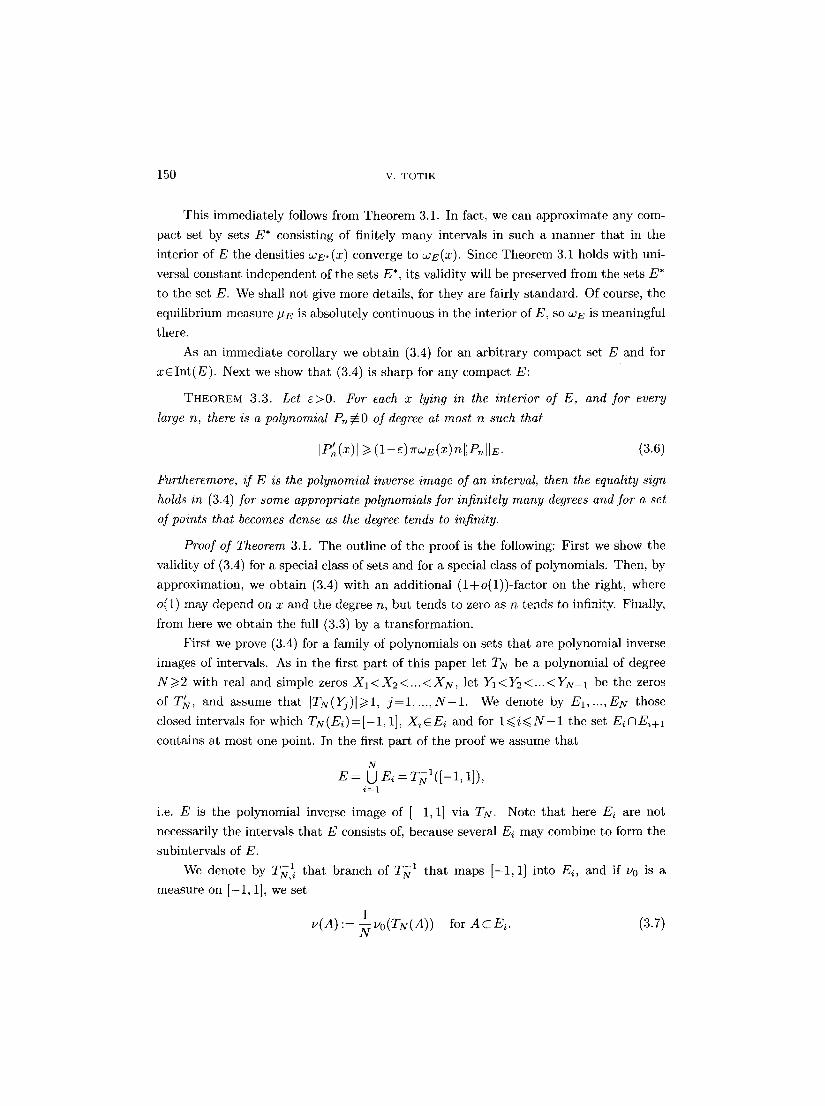
THEOREM 3.3. Let s:>0. For each x lying in the interior of E, and for every
large n, there is a polynomial P ,~O of degree at most n such that
[Ply(x)[ >1 (1--S)~WE(X)n[IPn[]E. (3.6)
Furtheremore, if E is the polynomial inverse image of an interval, then the equality sign
holds in (3.4) for some appropriate polynomials for infinitely many degrees and for a set
of points that becomes dense as the degree tends to infinity.
Proof of Theorem 3.1. The outline of the proof is the following: First we show the
validity of (3.4) for a special class of sets and for a special class of polynomials. Then, by
approximation, we obtain (3.4) with an additional ( l+o(1) ) - fae tor on the right, where
o(1) may depend on x and the degree n, but tends to zero as n tends to infinity. Finally,
from here we obtain the full (3.3) by a transformation.
First we prove (3.4) for a family of polynomials on sets that are polynomial inverse
images of intervals. As in the first part of this paper let TN be a polynomial of degree
N ~> 2 with real and simple zeros X] < X2 <... < XN, let Y1 < Y2 <--- < YN- 1 be the zeros
of T~, and assume that [TN(Yj)[~I , j = I , . . . , N - 1 . We denote by E1,...,EN those
closed intervals for which TN(Ei)=[-1, 1], XiEEi and for l~ i<~N-1 the set E~AE~+I
contains at most one point. In the first part of the proof we assume that
N
E = U Ei = TNI([--1, 1]), i = l
i.e. E is the polynomial inverse image of [ -1 , 1] via TN. Note tha t here Ei are not
necessarily the intervals that E consists of, because several Ei may combine to form the
subintervals of E.
T -1 that branch of TN 1 that maps [ -1 , 1] into Ei, and if v0 is a We denote by N#
measure on [--1, 1], we set
, (A) := luo(TN(A)) for ACE~. (3.7) / y
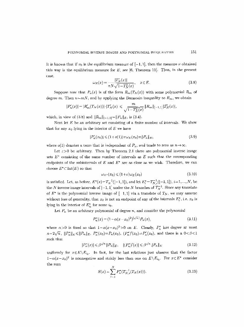
P O L Y N O M I A L I N V E R S E I M A G E S A N D P O L Y N O M I A L I N E Q U A L I T I E S 151
It is known that if u0 is the equilibrium measure of [ -1 , 1], then the measure u obtained
this way is the equilibrium measure for E, see [6, Theorem 11]. Thus, in the present
c a s e ,
~E(X) = IT;v(x)I x e E . (3.8)
Suppose now that Pn(x) is of the form Rm(TN(X)) with some polynomial Rm of
degree m. Then n=mN, and by applying the Bernstein inequality to Rm, we obtain
Ir~' (x)[ = IR'~(TN(X))I'ITfv(X)I <. m I[Rmll[-1,1] [T~(x)[, V / 1 - T ~ ( z )
which, in view of (3.8) and IIRmll[_l,1]=llPnllE, is (3.4).
Next let E be an arbi trary set consisting of a finite number of intervals. We show
that for any x0 lying in the interior of E we have
]P'~(xo)l ~< ( l+o( l ) )~E(xo)n t fP~ l lE , (3.9)
where o(1) denotes a te rm that is independent of Pn, and tends to zero as n-+oo.
Let c > 0 be arbitrary. Then by Theorem 2.1 there are polynomial inverse image
sets E* consisting of the same number of intervals as E such that the corresponding
endpoints of the subintervals of E and E* are as close as we wish. Therefore, we can
choose E*CInt(E) so that
~E*(Xo) <~ (l+e)a~E(X0) (3.10)
is satisfied. Let, as before, E*(x)=TNI([-1, 1]), and let E * = T ~ l i ( [ - 1 , 1]), i=1 , ..., N, be
the N inverse image intervals of [ -1 , 1] under the N branches of TN 1. Since any translate
of E* is the polynomial inverse image of [ -1 , 1] via a translate of TN, we may assume
without loss of generality, that x0 is not an endpoint of any of the intervals E~', i.e. x0 is
lying in the interior of E* for some i0. ~0
Let P~ be an arbi t rary polynomial of degree n, and consider the polynomial
P; (x) = ( 1 - ~ ( X - Xo)2)[~d] Pn(x), (3.11)
where c~>0 is fixed so that 1 - c ~ ( x - x 0 ) 2 > 0 on E. Clearly, P* has degree at most
n + 2 v ~ , IIPnllE<~llPnHE, P*(Xo)=P~(Xo), (P~)'(Xo)=P~(xo), and there is a 0 < Z < I
such that
IP*(z)l~</3'/~llP~llE, I(P~)'(x)l<~/3'/~llPnllE (3.12)
uniformly for xCE\Eio. In fact, for the last relations just observe that the factor
1 - a ( x - x 0 ) 2 is nonnegative and stricly less than one on E\Eio. For xfE* consider
the sum N
S(x) = E Pn(TN~ (TN(x)))" (3.13) i = 1
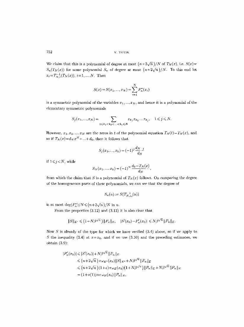
152 v. TOTIK
We claim that this is a polynomial of degree at most (n+2v~) /N of TN(X), i.e. S ( x ) =
Sn(TN(X)) for some polynomial S, of degree at most (n+2x/n)/N. To this end let
x~=TNI, i(TN(X)), i=1 , ..., N. Then
N
S ( x ) = S ( X l , . . . , XN) -~- E Pt:(zi) i = 1
is a symmetric polynomial of the variables xl, ..., XN, and hence it is a polynomial of the
elementary symmetric polynomials
Sj(Xl'""XN)= E XklXk2...Xkj, I<<.j<~N. l<~kt<k2<...<kj<~N
However, xl, x2, ..., XN are the zeros in t of the polynomial equation TN(t)=TN(X), and
so if TN(X)=dgxN+...+do, then it follows tha t
dN-j Sj(Xl '""xk)=(-1)J dN
if I<~j<N, while
SN(Xl, ...,Xk) = (--1) N dO-TN(x) dN
from which the claim that S is a polynomial of TN (x) follows. On comparing the degree
of the homogeneous parts of these polynomials, we can see that the degree of
Sn(u) := S(rNlio(u) )
is at most deg(P~)/N< ( n + 2 v ~ ) / N in u.
From the properties (3.12) and (3.13) it is also clear that
IISIIE- ~< ( I + N/~'/~ ) {{PnIIE, {S'(xo)- P;~(xo){ <<. N~'/~ IIPn{IE.
Now S is already of the type for which we have verified (3.4) above, so if we apply to
S the inequality (3.4) at x=xo, and if we use (3.10) and the preceding estimates, we
obtain (3.9):
{P'(x0)l ~< IS'(xo)I+N~ "/-~ IIP~IIE
<<. ( n + 2 ~ ) ~ E . ( X o ) I I S l I E . + N ~ IlPnlIE
<~ (n+ 2v~ )(l +e)TrwE(xo)(1 +N/~ v'~) IIPnlIE+ N~ v~ IlPn lIE
= (l+o(1))nTrwE(Xo)llPnllE,
P O L Y N O M I A L I N V E R S E IMAGES AND P O L Y N O M I A L I N E Q U A L I T I E S 153
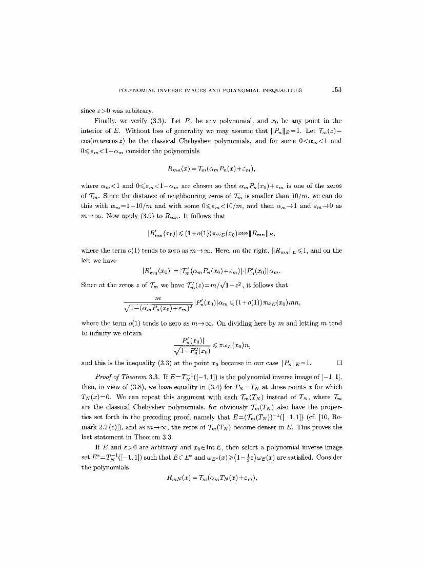
since c > 0 was arbitrary.
Finally, we verify (3.3). Let P~ be any polynomial, and x0 be any point in the
interior of E. Without loss of generality we may assume that IIPnllE=l. Let Tin(z)=
cos(marccosz) be the classical Chebyshev polynomials, and for some 0<c~m<l and
0 ~ g m < j- - - OLm consider the polynomials
l~mn(X) ='-]~m(O~rnPn(x)§
where c~m<l and O~Cm<l--ol m a r e chosen so tha t c~mP~(xo)+Cm is one of the zeros
of ~ . Since the distance of neighbouring zeros of Tm is smaller than 10/m, we can do
this with OLm--1-10/m and with some 0~<sm<10/m, and then O~m-+l and cm-+0 as
m--+oc. Now apply (3.9) to Rmn. It follows that
IlI~lrnn(XO)l ~ (l §
where the t e rm o(1) tends to zero as m--+c~. Here, on the right, IIRmnllE<~l, and on the
left we have
IR'n(X0)] = IT,~(c~mPn(xo)§ IP'n(XO)]am.
Since at the zeros z of Tm we have T ~ m ( Z ) = m / ~ , it follows that
m IP'(x0)l~m ~< (l+o(1))lrwE(xo)mn,
Jl--( mPn(xo)+ m) 2
where the te rm o(1) tends to zero as m--+oc. On dividing here by m and letting m tend
to infinity we obtain IP'(x0)l ~ ( x o ) n ,
v/1-p (xo) and this is the inequality (3.3) at the point x0 because in our c a s e HPnHE-=I. []
Proof of Theorem 3.3. If E = T N I ( [ - 1 , 1]) is the polynomial inverse image of [ -1 , 1],
then, in view of (3.8), we have equality in (3.4) for PN=TN at those points x for which
TN(X)=O. We can repeat this argument with each Tm(TN) instead of TN, where Tm
are the classical Chebyshev polynomials, for obviously Tm(TN) also have the proper-
ties set forth in the preceding proof, namely that E=(Tm(TN))-I([-1, 1]) (cf. [10, Re-
mark 2.2 (c)]), and as m--+oc, the zeros of T,~(TN) become denser in E. This proves the
last s ta tement in Theorem 3.3.
If E and ~>0 are arbi trary and x 0 E I n t E , then select a polynomial inverse image
set E * = T N I ( [ - 1 , 1]) such tha t ECE* and WE*(X)>~ (1--lC)WE(X) are satisfied. Consider
the polynomials
RmN(X) = Tm(amTN(X)§162
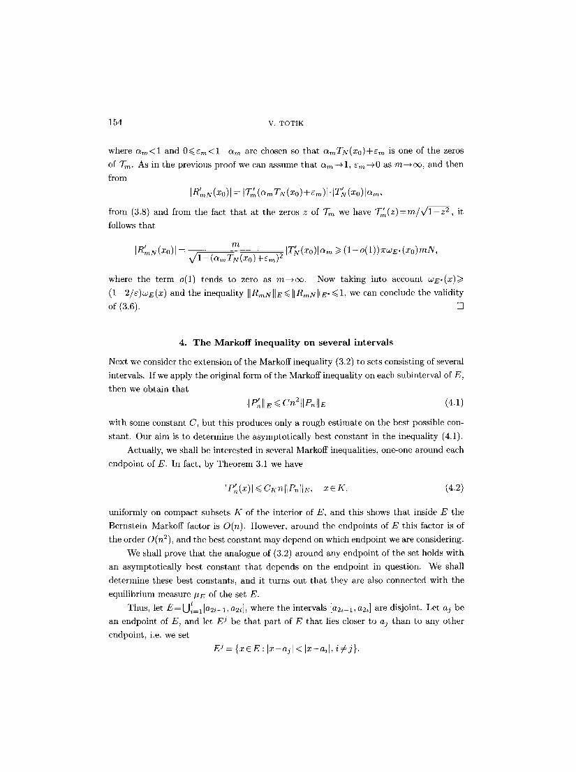
154 v. TOTIK
where a, ,~<l and 0 ~ < e m < l - a , ~ are chosen so that e~mTN(Xo)+e,~ is one of the zeros
of T,~. As in the previous proof we can assume that ct,,,-+1, am-+0 as rn--+oc, and then
f r o m
I R ~ N ( X O ) ] = V]'~lm(CtmTN(XO)-t-cm)l . ITIN(XO)IO~m,
from (3.8) and from the fact that at the zeros z of T,, we have T ~ ( z ) = m / ~ , it
follows tha t
IR:nN(xo)l = m I r ' N ( x o ) l c ' m ) (1--o(1))TrwE.(xo)mN,
where the term o(1) tends to zero as m-+oc . Now taking into account WE*(X)>~ (1--2/e)WE(X) and the inequality IIRmNIIE<~ IIRmNIIE �9 ~1, we can conclude the validity
of (3.6). []
4. T h e M a r k o f f i n e q u a l i t y on s e v e r a l i n t e r v a l s
Next we consider the extension of the Markoff inequality (3.2) to sets consisting of several
intervals. If we apply the original form of the Markoff inequality on each subinterval of E,
then we obtain that
IIP/~IIE ~< Cn I liP, liE (4.1)
with some constant C, but this produces only a rough estimate on the best possible con-
stant. Our aim is to determine the asymptotical ly best constant in the inequality (4.1).
Actually, we shall be interested in several Markoff inequalities, one-one around each
endpoint of E. In fact, by Theorem 3.1 we have
IP~(x)l ECKnflP, IIE, x c K , (4.2)
uniformly on compact subsets K of the interior of E, and this shows that inside E the
Bernstein-Markoff factor is O(n). However, around the endpoints of E this factor is of
the order O(n2), and the best constant may depend on which endpoint we are considering.
We shall prove tha t the analogue of (3.2) around any endpoint of the set holds with
an asymptotically best constant tha t depends on the endpoint in question. We shall
determine these best constants, and it turns out that they are also connected with the
equilibrium measure #E of the set E. l Thus, let E = U ~ = I [a2i-1, a2i], where the intervals [a2i-1, a2i] are disjoint. Let aj be
an endpoint of E, and let E j be that part of E that lies closer to ar than to any other
endpoint, i.e. we set
E j = { x e E : Ix-ajl < Ix-ail, iT~j}.
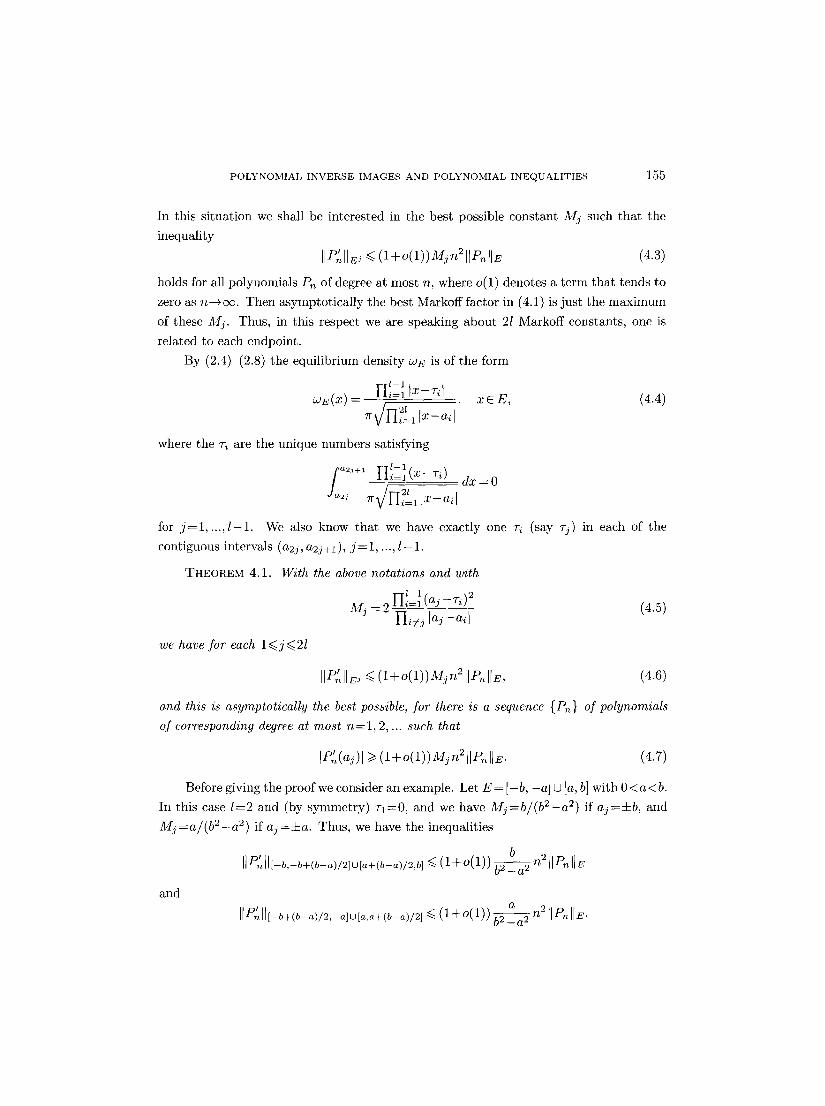
POLYNOMIAL INVERSE IMAGES AND POLYNOMIAL INEQUALITIES 155
In this situation we shall be interested in the best possible constant My such that the
inequality
IIP:~IIE~ ~< (l+o(1))Myn 2 [[PnlIE (4.3)
holds for all polynomials Pn of degree at most n, where o(1) denotes a term that tends to
zero as n--+ec. Then asymptotically the best Markoff factor in (4.1) is just the maximum
of these Mj. Thus, in this respect we are speaking about 21 Markoff constants, one is
related to each endpoint.
By (2.4) (2.8) the equilibrium density WE is of the form
II ~-' Ix-~ l WE(X) = 4=1 x E E, (4.4)
/~2~ Iz-a~l' V l l i = l
where the ri are the unique numbers satisfying
l--1 fo2~+~ 1-L=,(x-~d d x = O
V l l i = l
for j = l , . . . , l - 1 . We also know that we have exactly one 7=i (say Ty) in each of the
contiguous intervals (a2y, a2y+l), j = l , ..., l - 1 .
THEOREM 4.1. With the above notations and with
I--1 2 YIi=I (ay -~:i) (4.5)
Mj =_ i]i#-----j-laj_a---~
we have for each 1<<.j <~21
p ! II nllEJ ~ (l+o(1))Mj n211PnlIE, (4.6)
I[P;t[[[_b+(b_a)/2_a]U[a,a+(b_a)/2] ~ (1+o(1 ) ) a 2 b~--~j n IIP nllE.
and
and this is asymptotically the best possible, for there is a sequence {Pn} of polynomials of corresponding degree at most n=l , 2, ... such that
IP~(aj)l >~ (l +o(1) )Mjn211pnllE . (4.7)
Before giving the proof we consider an example. Let E = [-b, - a ] U [a, b] with 0 < a < b.
In this case l=2 and (by symmetry) 71=0, and we have Mj=b/(b2-a 2) if aj=+b, and
Mj=a/ (b2-a 2) if aj=• Thus, we have the inequalities
p' II n]l[--b,-b+(b--a)/2]U[a+(b--a)/2,b] <~ (1+O(1)) b n2 JIPnJJE
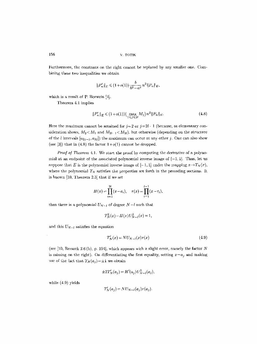
156 v. TOTIK
Furthermore, the constants on the right cannot be replaced by any smaller one. Com-
bining these two inequalities we obtain
IIP 'll (l+o(1)) T n211PnllE, E b - a
which is a result of P. Borwein [4].
Theorem 4.1 implies
IIP ' (l+o(1))( 2yj) llPnllE. (4.8)
Here the maximum cannot be attained for j = 2 or j = 2 / - 1 (because, as elementary con-
sideration shows, M2 < M1 and M21-1 < M2t), but otherwise (depending on the structure
of the l intervals [a2j-1, a2j]) the maximum can occur at any other j . One can also show
(see [3]) that in (4.8) the factor 1+o(1) cannot be dropped.
Proof of Theorem 4.1. We start the proof by computing the derivative of a polyno-
mial at an endpoint of the associated polynomial inverse image of [-1, 1]. Thus, let us
suppose that E is the polynomial inverse image of [ -1 , 1] under the mapping x-~ TN (x),
where the polynomial TN satisfies the properties set forth in the preceding sections. It
is known [10, Theorem 2.3] that if we set
2l l - -1
H ( x ) = l - I ( x - a d , r(x) = i = 1 i = 1
then there is a polynomial UN-I of degree N - 1 such that
T~ (x) - H(x) U2N_, (x) = 1,
and this UN-t satisfies the equation
= (4.9)
(see [10, Remark 2.6 (b), p. 194], which appears with a slight error, namely the factor N
is missing on the right). On differentiating the first equality, setting x=aj and making
use of the fact that TN(aj )=• we obtain
=H(aj)U _z(aj),
while (4.9) yields
T~(aj)=NUN_l(aj )r (a j ) .
P O L Y N O M I A L I N V E R S E I M A G E S AND P O L Y N O M I A L I N E Q U A L I T I E S 157
If we express from here U N _ 1 (%), and substitute the resulting equality into the previous
formula, then we obtain
vwl--1 / x2 ]T~ (aj)] = N 2. 2 IL=I [aj - T i) = N2Mj" (4.10)
I-Ii#j l a j - a i l
Next we verify (4.6) for the special case when E=TNI([-1, 1]) is the polynomial
inverse image of [-1, 1], and Pn is of the form Pn(x)=Rm(TN(X)). Let e>0 be arbitrary. Because of (4.2), for every ~>0 we have
liP" IIEJ\[aj-~,aj+wl ~< MJ n2 IIPnIIE
for sufficiently large n, and therefore it is enough to consider the r/-neighborhood of aj. We can choose this ~ so small that for x ~ [aj - rl, aj + 7/] we have I T~ (x)] ~< (1+ r (aj)l =
( I+r 2. Then for xE[aj-rl, aj+rl]nE we obtain from the classical Markoff in-
equality applied to the polynomial R,~ that
IP'~(x)t = IR'~(E~(x) )I'IT'N(x)I <~ m2NRmll[-a,ll(l +e)MjN 2 <~ (l +e)Mjn21lP~llE,
where we used that the norm of Rm over [-1, 1] coincides with the norm of P~ over E,
and that n=Nm.
Finally, let E be an arbitrary set consisting of a finite number of intervals. By
Theorem 2.1 we can choose a polynomial inverse image set E*= TNI([--1, 1]) consisting of
l intervals that lies arbitrarily close to E. Furthermore, in selecting E* we can also achieve
that aj is an endpoint of E*, and E * c E (see the remarks made after Theorem 2.1). It is
also true that the numbers 7-i are C~162 of the endpoints aj (see w hence we can
assume that if M] is the number Mj from (4.5) computed for E*, then M]<~(I+c)Mj, where e>0 is any given number. Now we can prove (4.6) for arbitrary Pn via polynomials
like P* and S(x) from (3.11) and (3.13) from the preceding section just as was done there.
In fact, let E*=TN,~([-1 , 1]), i=1, . . . ,N, be the inverse images under the N branches
of TN 1. Assume that ajEE~o , and let rj>0 be so small that [aj-r], aj+rI]NEcE~o and
this set does not contain the other endpoint of E]0. There are polynomials (see [16,
Theorem V1.3.6]) L / ~ of degree at most v ~ such that with some constants 0</3<1
and C we have
O<~ I - L v ~ ( x ) <~ C/TJ~ for xE[aj-rl , aj+rl] ,
0 ~< Lv~ (x) ~< C~ v~ for x E [.J E*, l<~i<~N, iT~jo
and otherwise 0~< Lv~ (x)~< 1 on E*. Instead of (3.11) consider the polynomial
P~(x)=L, /~(x)P,(x) , (4.11)
158 v TOTIK
which has similar properties as the P~ from (3.11), namely P,* has degree at most n + v ~ ,
IIP*I[E. <<.I]P,~IIE*, P*(x)=(I +O(~v~ ))P,~(x) for xE[aj--~,aj+~?],
I ( < ) ' ( x ) - < ( x ) l =O(n2/3"Za)llPnllE* for xE [aj-~,aj+~],
and
l<(x)l = o(m~)lIP~ll~., I(<)'(x)l = o (~2~) l lPnl lE .
uniformly for x E E* \Ei*o, where we have also used the classical Markoff inequality (3.2)
in the estimates of the derivatives. These show tha t if we define
N
S(x) : Z < (T;',(T~ (z))) i----1
as in (3.13), then exactly as after (3.13) we can conclude that this is a polynomial of TN, and
IISllE- ~< (I+O(~V-~))IIP,,IIE ., IS'(x)-P'(x)l <<. O(n2m'~)lIPnllE.
for all xc=E*M[aj-rhaj+rl]. Now S is already of the type for which we have verified
(4.6) above, so if we apply to S the inequality (4.6) and also take into account (4.2), then
we can conclude (4.6):
p' max(O(n)Hp,~ II nllE~ < liE*, ]lS'I[Emi~j-~,aj§ ~/~ [leslIE*)) <~ (l +o(1) )Mff (deg(S) ) 2 IlSllE.+O((n+n%~ )lIP. lIE-)
~< ( l+o(1)b2Mj IlPnlb" ~ (l+o(1))(l+c)n2Mj IIPnlIE,
where in the last step we used that E*cE and M~<~(I+a)M i. Since here c > 0 is
arbitrary, (4.6) follows.
The proof of (4.7) follows from the above considerations. In fact, as before, select a
polynomial inverse image set E * = T N 1([_ 1, 1]) consisting of I intervals tha t lies arbitrarily
close to E for which aj is an endpoint, and for which M~ is close to Mj, but now we
select E* so that it contains E. If T,~ are the classical Chebyshev polynomials, then
using that TN(aj)=+I, and [T'~(J=l)l=m 2, we get from (4.10) for m=[n/N]
I(Tm(TN ) )'(aj)I = m2N2M~,
and since here n2/m:N2--+l as n---+e~, and M~ is as close to Mj as we wish, (4.7)
follows. []

POLYNOMIAL INVERSE IMAGES AND POLYNOMIAL INEQUALITIES 159
R e f e r e n c e s
[1] ACHYESER, N. [AKHIEZER, N.I.], /Jber einige Funktionen, welche in zwei gegebenen Intervallen am wenigsten von Null abweichen. Bull. Acad. Sci. URSS Sdr. Math. (7) [Izv. Akad. Nauk SSSR Sdr. Math. (7)], 1932:9, 1163-1202.
[2] APTEKAREV, A.I., Asymptotic properties of polynomials orthogonal on a system of con- tours and periodic motions of Toda lattices. Mat. Sb. (N.S.), 125 (167) (1984), 231-258 (Russian); English translation in Math. USSR-Sb., 53 (1986), 223 260.
[3] BENK(~, D. ~ TOTIK, V., Sets with interior extremal points for the Markoff inequality. J. Approx. Theory, 110 (2001), 261-265.
[4] BORWEIN, P., Markov's and Bernstein's inequalities on disjoint intervals. Canad. J. Math., 33 (1981), 201 209.
[5] DEVORE, R.A. ~ LORENTZ, G.G. , Constructive Approximation. Grundlehren Math. Wiss., 303. Springer-Verlag, Berlin, 1993.
[6] GERONIMO, J.S. ~z VAN ASSCHE~ W:, Orthogonal polynomials on several intervals via a polynomial mapping. Trans. Amer. Math. Soc., 308 (1988), 559 581.
[7] LANDKOF, N. S., Foundations of Modern Potential Theory. Grundlehren Math. Wiss., 180. Springer-Verlag, NewYork, 1972.
[8] PEHERSTORFER, F., On Bernstein Szeg5 orthogonal polynomials on several intervals, I. SIAM J. Math. Anal., 21 (1990), 461 482.
[9] - - On Bernstein-Szeg5 orthogonal polynomials on several intervals, II. Orthogonal poly- nomials with periodic recurrence coefficients. J. Approx. Theory, 64 (1991), 123 161.
[10] Orthogonal and extremal polynomials on several intervals. J. Comput. Appl. Math., 48 (1993), 187 205.
[11] - - Elliptic orthogonal and extremal polynomials. J. London Math. Soc. (3), 70 (1995), 605 624.
[12] - - Approximation of several intervals by an inverse polynomial mapping. To appear in J. Approx. Theory.
[13] PEHERSTOREER, F. ~z SCHIEFERMAYR, K., Description of extremal polynomials on several invervals and their computation, I. Acta Math. Hungar., 83 (1999), 27-58.
[14] PEHERSTOREER, F. ~ STEINBAUER, R., On polynomials orthogonal on several intervals. Ann. Numer. Math., 2 (1995), 353-370.
[15] RANSFORD, W., Potential Theory in the Complex Plane. London Math. Soc. Stud. Texts, 28. Cambridge Univ. Press, Cambridge, 1995.
[16] SAFF, E. B. & TOTIK, V., Logarithmic Potentials with External Fields. Grundlehren Math. Wiss., 316. Springer-Verlag, Berlin, 1997.
[17] STAHL, H. ~: TOTIK, V., General Orthogonal Polynomials. Encyclopedia Math. Appl., 43. Cambridge Univ. Press, Cambridge, 1992.
[18] SZEGS, G., Uber einen Satz des Herrn Serge Bernstein. Schr. K5nigsberg. Gel. Ges., 5 (1928/29), 59 70.
[19] TIMAN, A. F., Theory of Approximation of Functions of a Real Variable. Dover, NewYork, 1994.
[20] TsuJI, M., Potential Theory in Modern Function Theory. Maruzen, Tokyo, 1959. [21] WIDOM, H., Extremal polynomials associated with a system of curves in the complex plane.
Adv. Math., 3 (1969), 127-232.

160 V. TOTIK
VILMOS TOTIK Bolyai Institute University of Szeged Aradi v. tere 1 HU-6720 Szeged Hungary
and
Department of Mathematics University of South Florida Tampa, FL 33620 U.S.A. totik~math.usf.edu
Received September 24, 1999