polynomial-time solution of prime factorization and np ... · np-hard problems with digital...
TRANSCRIPT
1
Polynomial-time solution of prime factorization andNP-hard problems with digital memcomputing
machinesFabio L. Traversa, Massimiliano Di Ventra
Abstract—We show how to solve the prime factorizationand the NP-hard version of the subset-sum problem on digitalmemcomputing machines using polynomial resources. We firstintroduce the complexity classes for these machines, make aconnection with dynamical systems theory, and propose a prac-tical scheme to solve the above problems based on the novelconcept of self-organizable logic gates and circuits. These arelogic gates and circuits that can solve boolean problems by self-organizing into their solution. They can be fabricated eitherwith circuit elements with memory (such as memristors) and/orstandard MOS technology. Using tools of functional analysis, weprove that these machines have a global attractor and the onlyequilibrium points are the solution(s) of the above problems.In addition, any initial condition converges exponentially fast tothe solution(s), and the equilibrium convergence rate scales atmost polynomially with input size. Since digital memcomputingmachines map integers into integers they are robust against noise,and hence scalable. Therefore, they are a realistic alternativeto Turing machines to efficiently solve very complex problems.We finally discuss the implications of our results to the NP=Pquestion.
Index Terms—memory, memristors, elements with memory,memcomputing, Turing Machine, NP-complete, subset-sum prob-lem, factorization, dynamical systems, dissipative systems, globalattractor.
I. INTRODUCTION
We have recently shown that a new class of non-Turingmachines, we have named Universal Memcomputing Ma-chines (UMMs), has the same computational power of non-deterministic Turing machines, and as such they can solve (ifimplemented in hardware) NP-complete/hard problems withpolynomial resources [1]. UMMs are machines composedof interacting memprocessors, namely processors that usememory to both process and store information on the samephysical location [2]. Their computational power rests ontheir intrinsic parallelism - in that the collective state of themachine (rather than the individual memprocessors) computes- and their information overhead: a type of information that isembedded in the machine but not necessarily stored by it [1].
The information overhead is the direct result of the topologyof the network of memprocessors, and can be appropriately“tuned” to the complexity of the problem. For instance,problems that would otherwise require exponential resourceswith a standard deterministic Turing machine, require only
The authors are with the Department of Physics, University of California-San Diego, 9500 Gilman Drive, La Jolla, California 92093-0319, USA, e-mail:[email protected], [email protected]
polynomial resources with a UMM if we feed into it an expo-nential information overhead through the appropriate topology.
We have already provided a practical example of such amachine that solves the NP-complete version of the subset-sumproblem in one computational step using a linear number ofmemprocessors and built it using standard electronic compo-nents [3]. However, the machine we have built is fully analogand as such can not be easily scaled up to an arbitrary numberof memprocessors without noise control. However, UMMs canalso be defined in digital mode and if a practical scheme can beengineered to realize them in practice, we could build scalablemachines that solve very complex problems using resourcesthat only grow polynomially with input size.
In this paper we suggest such a scheme and apply it totwo important problems: prime factorization and the NP-hardversion of the subset-sum problem. However, we accomplishmore than just solving these two problems. The list of majorresults of our paper, with the corresponding sections wherethe reader can find them, are as follows.• We define the types of problems that we are interested in
and the computational protocols we have in mind whichwill be important in practical realizations. Section II.
• We define digital memcomputing machines (DMMs) andtheir complexity classes. Section III.
• We formulate DMMs in terms of the theory of dynamicalsystems in order to make the transition from mathematicalconcept to physical systems and hence facilitate theirpractical realization. Section IV.
• We introduce the notion of self-organizable logic gatesand self-organizable logic circuits, namely gates andcircuits that, through the collective state of the machine,can satisfy boolean functions in a self-organized manner.Section V.
• Using tools of functional analysis, we demonstrate an-alytically that the dynamical systems describing thesecircuits are dissipative and hence support a global at-tractor [4]. In addition, we prove that i) their equilibriaare the solutions of the problems they represent, ii)any initial condition converges exponentially fast to thesolution(s), iii) the equilibrium convergence rate scalesat most polynomially with input size, iv) the energyexpenditure only grows polynomially with input size, andv) we provide arguments and numerical evidence thatperiodic orbits and strange attractors cannot coexist withequilibria. Section VI.
• We support the above results with numerical simulations
arX
iv:1
512.
0506
4v1
[cs
.ET
] 1
6 D
ec 2
015

2
of the solution of prime factorization and the subset-sum problem using DMMs with appropriate topologies.Section VII.
• We discuss the consequences of our results on the ques-tion of whether NP=P. Section VIII.
Finally, Section IX collects our thoughts for future direc-tions in the field.
II. PRELIMINARY DEFINITIONS
Before defining the DMMs, we introduce the general classof problems we want to tackle. This will clarify the type ofapproach we will use to solve them, and will lead us to thedefinition of the machines’ computational complexity classes.
A. Compact Boolean Problems
Definition II.1 A Compact Boolean problem is a collection ofstatements (not necessarily independent) that can be written asa finite system of boolean functions. Formally, let f : Zn2 →Zm2 be a system of boolean functions and Z2 = {0, 1}, thena CB problem requires to find a solution y ∈ Zn2 (if it exists)of f(y) = b with b ∈ Zm2 .
It is clear from this definition that this class includesmany important problems in Computer Science, such as theNondeterministic Polynomial- (NP-) time problems, linearalgebra problems, and many others. For instance, such a classincludes those we solve in Sec. VII, namely factorization andthe subset-sum problem.
B. Direct and Inverse Protocols
We further define two ways (protocols) to find a solution ofsuch problems. The first one can be implemented within theTuring machine paradigm through standard boolean circuits.The second one can only be implemented with DMMs.
Definition II.2 Let SB = {g1, . . . , gk} be a set of k booleanfunctions gj : Znj2 → Zmj2 , SCFS = {s1, . . . , sh} a set of hcontrol flow statements, and CF the control flow that specifiesthe sequence of the functions gj ∈ SB to be evaluated and thestatements sj ∈ SCFS to be executed. We then define theDirect Protocol (DP) for solving a CB problem that controlflow CF which takes y′ ∈ Zn
′
2 as initial input and givesy ∈ Zn2 as final output such that f(y) = b.
Roughly speaking, the DP is the ordered set of instructions(the program) that a Turing machine should perform to solvea CB problem. Even if a DP is not the unique way to finda solution of a given CB problem with Turing machines,all the other known strategies (even if they are, possibly,more optimal) do not change the computational complexityclasses of Turing machines. For this reason, we consider hereonly DPs as some general Turing-implementable strategies forsolving CB problems.
Boolean functions are not, in general, invertible and findingthe solution of a CB problem is not equivalent to finding thezeros of a vector function f because the solution belongs toZn2 and not to Rn or Cn. Nevertheless, we can still thinkof a strategy to find the solution of a CB problem that can
be implemented in a specific machine. This means that themachine must be designed specifically to solve only such a CBproblem. We will give explicit examples of such machines inSec. VII when we solve factorization and the NP-hard versionof the subset-sum problem. We then define:
Definition II.3 An Inverse Protocol (IP) is that which findsa solution of a given CB problem by encoding the booleansystem f into a machine capable of accepting as input b, andgiving back as output y, solution of f(y) = b.
Roughly speaking, the IP is a sort of “inversion” of f usingspecial-purpose machines.
C. Algorithmic Boolean Problems
Of course, the definition of CB problems does not exaust allpossible problems in Computer Science. We can also definethe following class:
Definition II.4 The Algorithmic Boolean (AB) problems arethose problems described by a collection of statements mathe-matically formalized by a control flow with boolean functionsand appropriate control flow statements.
The CB problems are clearly a subclass of AB problems.However, it is not easy to say a priori if an AB problemcan be reduced to a CB problem. For example, control flowsincluding loops that terminate only if a condition is metcannot be always translated into a finite system f of booleanfunctions. Moreover, the same problem that can be formulatedeither as CB or AB, may not have the same complexity inthe respective formulation. For example, in order to reducef to a unique boolean system, if we consider a control flowCF that requires the evaluation of nB boolean functions andnC conditional branches (i.e., the “if-then” statements thatare a specific case of control flow statements), we may needresources increasing with the dimension of f which, in turn,increases non-polynomially with nC . More insights will begiven in Sec. III-B.
We remark that by the term resources we denote the amountof space, time, and energy employed by the machine. Finally,we only acknowledge that there exist problems that cannot beclassified as AB. These are beyond the scope of our presentpaper and therefore will not be treated here.
III. DIGITAL MEMCOMPUTING MACHINES
We are now ready to define the digital versions of mem-computing machines (DMMs). These are a special class ofUniversal Memcomputing Machines (UMMs) we have intro-duced in Ref. [1] in which the memprocessors (processors withmemory) have only a finite number of possible states afterthe transition functions, δs, have been applied. Note that thetransition functions can be implemented using, e.g., circuits(as we will show later) or some other physical mechanism.The important point is that they map Zn2 into Zm2 , with n andm arbitrary integers.
A. Formal definition
We recall that the UMM is an ideal machine formed bya bank of m interconnected memory cells – memprocessors

3
memprocessors
input (y)
output (b)
Topology of connections encoding f
memprocessors
input (b)
output (y)
Topology of connections encoding f
(a) TEST MODE (b) SOLUTION MODE
‒1
Fig. 1. Sketch of a DMM. The memprocessors are two-state interconnectedelements that change their state according to both the external signal fed bythe Control Unit and the signals from the other memprocessors through theirconnections. δ is the composition of all transition function involved in thecomputation. The (a) panel shows the test mode for the verification of a givensolution of a CB problem, while the (b) panel the solution mode for the IPimplementation.
– with m ≤ ∞. Its DMM subclass performs digital (logic)operations controlled by a control unit (see Fig. 1). Thecomputation with and in memory can be sketched in the fol-lowing way. When two or more memprocessors are connected,through a signal sent by the control unit, the memprocessorschange their internal states according to both their initial statesand the signal, thus giving rise to intrinsic parallelism (inter-acting memory cells simultaneously and collectively changetheir states when performing computation) and functionalpolymorphism (depending on the applied signals, the sameinteracting memory cells can calculate different functions) [1].The information overhead typical of UMMs will be defined atlength in Sec. III-E.
Definition III.1 A DMM is the eight-tuple
DMM = (Z2,∆,P, S,Σ, p0, s0, F ) . (1)
Without loss of generality, we restrict the range to Z2 = {0, 1}because the generalization to any finite number of states istrivial and does not add any major change to the theory. ∆ isa set of functions
δα : Zmα2 \F × P → Zm′α
2 × P2 × S , (2)
where mα <∞ is the number of memprocessors used as inputof (read by) the function δα, and m′α < ∞ is the numberof memprocessors used as output (written by) the functionδα; P is the set of the arrays of pointers pα that select thememprocessors called by δα and S is the set of indexes α; Σis the set of the initial states written by the input device on thecomputational memory; p0 ∈ P is the initial array of pointers;s0 is the initial index α, and F ⊆ Zmf2 for some mf ∈ N isthe set of final states.
AB CB PCM NPCM
MPIMPIM
NPIM
Fig. 2. Euler diagram of computatinal complexity classes with respect todigital memcomputing machines. Of all problems AB = Algorithmic Boolean,the subclass CB = Compact Boolean can be solved in time PCM = Polyno-mially Compact, NPCM = Non-Polynomially Compact, PIM = PolynomiallyInvertible, MPIM = Memcomputing Polynomially Invertible, NPIM = Non-Polynomially Invertible. Note that PCM=PIM ∪ MPIM ∪ NPIM.
B. Computational complexity classes
We now use the notion of AB and CB problems introducedin Sec. II to define the first two classes of computationalcomplexity for a DMM. It is again worth recalling for thesubsequent definitions that a DMM can be used also asa standard Turing machine when implemented in DP (see[1] for more details). It implies that we can design DMMsto implement problems in their AB formulation as well asdesigning other DMMs implementing problems in their CBformulation.
Definition III.2 A CB problem is said to be PolynomiallyCompact for a DMM (PCM) if, for a given y ∈ Zn2 , to verify ify satisfies f(y) = b both the DMM implementing f(y) andthe DMM implementing the CF from the AB formulation ofthe problem, require polynomial resources in n.
Conversely,
Definition III.3 a CB problem is said to be Non-PolynomiallyCompact for a DMM (NPCM) if, for a given y ∈ Zn2 , toverify if y satisfies f(y) = b the DMM implementing f(y)requires more than polynomial resources in n while the DMMimplementing the CF from the AB formulation of the problemrequires only polynomial resources.
We can further define other three computational complexityclasses based on the complexity of the DP and IP.
Definition III.4 A CB problem is said to be PolynomiallyInvertible for a DMM (PIM), if, to find a solution y off(y) = b with both the DP and the IP requires polynomialresources in n = dim(b).
On the other hand,
Definition III.5 a CB problem is said to be MemcomputingPolynomially Invertible for a DMM (MPIM) if, to find asolution y of f(y) = b with a DP requires more than poly-nomial resources in n, while the IP requires only polynomialresources.
On the contrary,
Definition III.6 a CB problem is said to be Non-PolynomiallyInvertible for a DMM (NPIM) if, to find a solution y of f(y) =

4
b with both the DP and the IP requires more than polynomialresources in n = dim(b).
Finally, we remark that the case in which the IP requiresmore than polynomial resources while the DP only polynomialresources belongs to NPCM, and the case in which bothrequire more than polynomial resources belongs to CB\PCM.However, both instances are not of interest to the present work.Therefore, we do not define them here. The Euler diagram ofthe complexity classes for DMMs is shown in Fig. 2.
C. Topological implementation of IP within DMMs
A DMM can be designed either to implement the DP orthe IP. We discuss only the implementation of the latter casesince the implementation of the DP is the same as for Turingmachines so it does not add anything new.
We focus on a given CB problem characterized by theboolean system f . Since f is composed of boolean functions,we can map f into a boolean circuit composed of logic gates.Then, implementing f into a DMM can be formally doneby mapping the boolean circuit into the connections of thememprocessors. The DMM can then work in two differentmodes: test and solution modes (see Fig. 1).
In the test mode (see panel (a) of Fig. 1) the control unitfeeds the appropriate memprocessors with a signal encodingy. In this way, the first transition function δα receives itsinput. Performing the composition of all transitions functions,(δζ ◦ · · · ◦ δα)(y), we obtain the output f(y) to be comparedagainst b to determine whether or not y is a solution of the CBproblem. In this case, the transition function δ = δζ ◦ · · · ◦ δαrepresents the encoding of f through the topology of theconnections of the memprocessors.
Conversely, in the solution mode (see panel (b) of Fig. 1)the control unit feeds the appropriate memprocessors with asignal encoding b. The first transition function δ−1α receives itsinput, and the composition of all transitions functions, (δ−1ζ ◦· · · ◦ δ−1α )(b), produces the output y.
The transition function δ−1 = δ−1ζ ◦· · ·◦δ−1α still representsthe encoding of f through the topology of the connections ofthe memprocessors. However, it works as some system g suchthat g(b) = y. Note that g is not strictly the inverse of fbecause it may not exist as a boolean system. For this reasonwe call g the topological inverse of f and δ−1 the topologicalinverse transition function of δ.
D. Some remarks
We add here some remarks to better understand how DMMsoperate. As we have seen, the DMM works by encodinga boolean system f onto the topology of the connections.It means that to solve a given problem with a given inputlength we must use a given DMM formed by a number ofmemprocessors and topology of connections directly relatedto f and the input length. Furthermore, we notice that thepossibility of implementing the IP to solve a CB problem intoa DMM is ultimately related to its intrinsic parallelism [1].Finally, even if the realization of such particular DMM is notunique (there may be different types of memprocessors and
topologies that solve such a problem) it is, however, a specialpurpose machine designed to solve a specific problem.
Conversely, the Turing machine is a general purpose ma-chine in the sense that to solve a given problem we have toprovide a set of instructions to be computed. In other words,the Turing machine can only solve problems employing theDP. It is also worth remarking that DMMs are more thanstandard neural networks (even if a neural network is a specialcase of DMMs). In fact, artificial neural networks do notfully map the problems into the connectivity of neurons. Onthe contrary, they are in some measure “general purpose”machines that need to be trained to solve a given problem.The DMM transfers the network training step into the choiceof network topology.
Finally, we provide some considerations on the possiblestrategy to device cryptographic schemes for DMMs. As weshow in Sec. VII, NP problems such as factorization or thesubset-sum problem, can be efficiently solved with DMMsimplementing the IP. It means that the standard cryptosystemslike the RSA [5] or others based on the notion that NPproblems provide possible one-way functions [6], can bebroken by DMMs. We then have to look at new cryptosystemsbeyond the Turing machine paradigm. As a guideline wenotice here that a cryptosystem for DMMs should be basedon problems belonging either to the class NPIM or NPCM thathave both the DP and IP scaling more than polynomial in thelength of the input. However, the class of the NPIM problemscould be empty if all the PCM problems can be solved inpolynomial time by the DMM employing the IP. In this case,we should instead focus on NPCM problems.
E. Information Overhead
Using the definition given in the previous sections, we cannow formally define a concept that we already have introducedin [1]: the information overhead. We first stress that thisinformation is not stored in any memory unit. The storedinformation is the Shannon self-information that is equal forboth Turing machines and UMMs. Instead, it represents theextra information that is embedded into the topology of theconnections of the DMMs. Thus we have:
Definition III.7 The information overhead is the ratio
IO =
∑i(m
Uαi +m′Uαi)∑
j(mTαj +m′Tαj )
, (3)
where mTαj and m′Tαj are the number of memprocessors read
and written by the transition function δTαj that is the transitionfunction of a DMM formed by interconnected memprocessorswith topology of connections related to the CB problem, whilemUαi and m′Uαi are the number of memprocessors read and
written by the transition function δUαi that is the transitionfunction of a DMM formed by the union of non-connectedmemprocessors. The sums run over all the transition functionsused to find the solution of the problem.
From this definition, if we use the IP, δTαj = δ−1αj defined insection III-C. Conversely, since δUαi is the transition functionof non-connected memprocessors the unique way to find a
5
solution is by employing the DP. Therefore, problems belong-ing to the class MPIM have information overhead that is morethan polynomial, i.e., the topology encodes or “compresses”much more information about the problem than the DP. It isworth noticing again that this information is something relatedto the problem, i.e., related to the structure of f (topologyof the memprocessor network), and not some actual datastored by the machine. Finally, due to its different nature, theinformation overhead that we have defined does not satisfythe standard mathematical properties of information measures(see Sec.IV-C). Instead, it provides a practical measure of theimportance of the topology in a given computing network.
IV. DYNAMICAL SYSTEMS PICTURE
In order to provide a practical, physical route to implementDMMs, we now reformulate them in terms of dynamicalsystems. This formulation will also be useful for a formal defi-nition of accessible information and information overhead (thelatter already introduced in [1]) and at the same time to clearlypoint out their scalability and main differences with the mostcommon definitions of parallel Turing machines. Note that adynamical systems formulation has also been used to discussthe computational power of analog neural networks [7], [8],which can be classified as a type of memcomputing machinesthat have no relation between topology and the problem tosolve. Here, we extend it to DMMs proper.
A. Dynamical systems formulation of DMMs
We consider the transition function δα defined in (2) andpα, p
′α ∈ P being the arrays of pointers pα = {i1, ..., imα}
and p′α = {j1, ..., jm′α}. Furthermore, we describe the state of
the DMM (i.e., the state of the network of memprocessors)using the vector x ∈ Zn2 . Therefore, xpα ∈ Zmα2 is the vectorof states of the memprocessors selected by pα. Then, thetransition function δα acts as:
δα(xpα) = x′p′α , (4)
In other words, δα reads the states xpα and writes the newstates x′p′α , both belonging to Zn2 . Equation (4) points outthat the transition function δα simultaneously acts on a setof memprocessors (intrinsic parallelism).
The intrinsic parallelism of these machines is the featurethat is at the core of their power. It is then very important tounderstand its mechanism and what derives from it. To analyzeit more in depth, we define the time interval Iα = [t, t +Tα] that δα takes to perform the transition. We can describemathematically the dynamics during Iα making use of thedynamical system framework [9]. At instant t the control unitsends a signal to the computational memory whose state isdescribed by the vector x(t). The dynamics of the DTM withinthe interval Iα between two signals sent by the control unit isdescribed by the flow φ (the definition of flow follows fromthe dynamical systems formalism [9])
x(t′ ∈ Iα) = φt′−t(x(t)), (5)
namely all memprocessors interact at each instant of time inthe interval Iα such that
xpα(t) = xpα (6)xp′α(t+ Tα) = x′p′α (7)
B. Parallel Turing Machines
In [10] we have briefly discussed the parallelism in today’scomputing architectures, i.e., Parallel Turing Machines (PTM).Here, for the sake of completeness, we summarize the mainresults useful to compare against the intrinsic parallelism ofDMMs.
Parallelism in standard computing machines can be viewedfrom two perspectives: the practical and the theoretical one.The theoretical approach is still not well assessed and there aredifferent attempts to give a formal definition of PTMs [11]–[18]. Irrespective, the PTM often results in an ideal machinethat cannot be practically built [14], [16]. Therefore, we aremore interested in a description of the practical approach toparallelism.
The definition we give here includes some classes of PTMs,in particular the Cellular Automata and non-exponentiallygrowing Parallel Random Access Machines [11]–[13], [18].We consider a fixed number of (or at most a polynomiallyincreasing number of) central processing units (CPUs) thatperform some tasks in parallel. In this case each CPU canwork with its own memory cash or accesses a shared memorydepending on the architecture. In any case, in practical ParallelMachines (PM), all CPUs are synchronized, each of themperforms a task in a time TPM (the synchronized clock ofthe system of CPUs), and at the end of the clock cycle allCPUs share their results and follow with the subsequent task.We can describe mathematically also this picture within thedynamical system framework [9] to point out the differencewith the intrinsic parallelism of memcomputing.
Let us consider the vector functions s(t) =[s1(t), ..., sns(t)] and k(t) = [k1(t), ..., knk(t)] definingrespectively the states of the ns CPUs and the symbolswritten on the total memory formed by nk memory units. Aslong as the CPUs perform their computation, at each clockcycle they act independently so there are ns independentflows describing the dynamics during the computation ofthe form (sj(t + TPM), kjw(t + TPM)) = φjTPM
(sj(t),k(t))where kjw is the memory unit written by the j-th CPU.Since the j-th CPU just reads the memory k(t) at only thetime t and not during the interval IPM =]t, t + TPM], and itdoes not perform any change on it apart from the unit kjw ,the evolution of the entire state during IPM is completelydetermined by the set of independent equations
(sj(t′ ∈ IPM),mjw(t′ ∈ IPM)) = φjt′−t(sj(t),k(t)), (8)
which a quick comparison with Eq. 5 shows the fundamentaldifference with memcomputing machines: in each interval IPMthe ns CPUs do not interact in any way and their dynamicsare independent.

6
C. Accessible Information
Let us now consider a DMM and a PTM having thesame number, m, of memprocessors, and standard processors,respectively, and taking the same time T to perform a stepof computation. Moreover, we can also assume that at time tand t+ T , the computing machines (whether DMM or PTM)have the state of the memory units that can be either 0 or 1.Therefore, the number of all possible initial or final configura-tions of both the DMM and PTM is 2m, and the Shannon self-information is equal for both, namely IS = − log2[2−m] = m.We introduce the
Definition IV.1 The accessible information IA is the volumeof the configuration space explored by the machine during thecomputation, i.e., during the interval IT .
We remark that the concept and definition of accessibleinformation (and also of information overhead given in sec-tion III-E), even if it follows from principles of statisticalmechanics, it is not the standard information measure in thesense that it does not satisfy the usual properties of theinformation measures. On the other hand, our definition is ableto highlight relevant features useful to point out differencesbetween DMMs (or UMMs in general) and Turing machines.For instance, from (8), the PTM is equivalent to a system ofm non-interacting objects, so from the principles of statisticalmechanics [19] the number of total configurations is the sumof the configurations allowed for each individual element, i.e.,2m, and hence the volume of the configuration space exploredduring the computation is also 2m. The accessible informationin this case is then IA ∝ 2m. On the other hand, in the case ofDMMs, we have that the memprocessors interact and followthe dynamics (5), therefore the volume of configuration spaceexplored by a DMM during I is 2m and IA ∝ 2m.
D. Information Overhead vs. Accessible Information
We have introduced the concept of information overheadin [1] and formalized it in the problem/solution picture inSec. III-E. In this section we discuss its relationship with theaccessible information making use of the dynamical systemspicture.
As described above, the DMMs can access, at each com-putational step, a configuration space that may grow exponen-tially. Therefore, a DMM, even if it starts from a well definedconfiguration and ends in another well defined configurationboth belonging to Zm2 , during the computation its collectivestate (i.e., the state of the memprocessor network) results in asuperposition of all configurations allowed by the DMM.
We consider a unit proportionality coefficient between thevolume of the explored configuration space by the machineand the accessible information as defined in Sec. IV-C. Now,the accessible information is always larger or equal to thenumber of memprocessors involved in the computational step.In fact, we have 2m ≤ IA ≤ 2m and (mα + m′α) ≤ 2m andthen (mα+m′α) ≤ IA. Therefore, using equation (3), we have
IO ≤∑i IUAi∑
j(mTαj +m′Tαj )
, (9)
where IUAi is the accessible information of the computationalstep i of a DMM formed by a union of non-connectedmemprocessors.
We can further notice that IUAi = 2mUi ≥ (mU
αi + m′Uαi)where mU
i is the total number of memprocessors involvedin the computational step i. Conversely, the accessible infor-mation of the computational step j of a DMM formed byinterconnected memprocessors is ITAj = 2m
Tj .
Now, we consider a CB problem belonging to PCM withn = dim(b) and f the associated boolean system. Bythe definitions in Sec. III-B, the number of memprocessorsinvolved in the computation (either in test or solution mode)is a polynomial function of n. Moreover, the number ofsteps to solve a problem in MPIM is polynomial for the caseof IP (namely when interconnected memprocessors encodef into the topology of the connections) while it could bemore than polynomial in the case of DP (for examples, theunion of non-connected memprocessors). Then, there existtwo positive polynomial functions P (n) and Q(n) such thatP (n)
∑i IUAi = Q(n)
∑j I
TAj . We can substitute this relation
into Eq. (9) and have (since all quantities are related to thesame machine we can suppress the superscript T ):
IO ≤Q∑j IAj
P∑j(mαj +m′αj )
. (10)
It is worth noticing that the relation (10) is valid for anytype of topology, including the one with no connections. Infact, in the case of no connections and computational steps thatinvolve all memprocessors (which is equivalent to a PTM) wehave that P = Q, IAj = 2mj = (mαj + m′αj ) and IO ≤ 1,namely, no information has been encoded (compressed) intothe topology of the machine.
The other limit case is that of connections not related tothe problem (like in neural networks). In this case, at leastone of P or Q cannot be polynomial but the ratio P/Q mustbe more than polynomial in n and the IO is maximized by apolynomial function of n.
E. Equilibrium points and IP
The information overhead and accessible information de-fined in the previous section can be interpreted as operationalmeasures of the computing power of a DMM. However,another important feature to characterize the computing powerof the DMMs is the composition of its phase space, i.e.,the n-dimensional space in which x(t) is a trajectory (notto be confused with the configuration space). In fact, theextra information embedded into a DMM by encoding f ontothe connection topology strongly affects the dynamics of theDMM, and in particular its global phase portrait, namely thephase space and its regions like attraction basins, separatrix,etc. [9].
To link all these concepts, we first remark that the dynamicalsystem describing a DMM should have the following proper-ties:• each component xj(t) of x(t) has initial conditionsxj(0) ∈ X , where X is the phase space and also a metricspace,

7
• to each configuration belonging to Zm2 , one or moreequilibrium points xs ∈ X can be associated, and thesystem converges exponentially to these equilibria [4],
• the stable equilibria xs ∈ X are associated to thesolutions of the CB problem,
• to coherently define the DMM as a digital machine, theinput and output of the DMM (namely y and b in testmode or b and y in solution mode) must be mapped intoa set of parameters p (input) and equilibria xs (output)such that ∃ p, x ∈ R and |pj − p| = cp and |xsj − x| =cx for some cp, cx > 0 independent of ny = dim(y)and n = dim(b). Moreover, if we indicate a polynomialfunction of n of maximum degree γ with pγ(n), thendim(p) = pγp(n) and dim(xs) = pγx(nb) in test modeor dim(p) = pγp(nb) and dim(xs) = pγx(n) in solutionmode, with γx and γp independent of nb and n.
• other stable equilibria, periodic orbits or strange attractorsthat we generally indicate with xw(t) ∈ X , not associatedwith the solution(s) of the problem, may exist, but theirpresence is either irrelevant or can be accounted for withappropriate initial conditions.
• The system has a compact global asymptotically stableattractor [4], which means that it exists a compact J ⊂ Xthat attracts the whole space X (for the formal definitionsee Sec. VI-F).
It is worth noticing that the last requirement implies thatthe phase space is completely clustered in regions that arethe attraction basins of the equilibrium points and, possibly,periodic orbits and strange attractors, if they exist. We alsopoint out that a class of systems that has a global attractoris the one of dissipative dynamical systems [4]. We will givea more detailed description of them in Sec. VI-F. We willalso show in Sec. VI-G that all the examples we providesatisfy these properties with the added benefit that the onlyequilibrium points are the solutions of the problem.
We further define V = vol(X) the hyper-volume of Vdefined by some Lebesgue measure on X , Js ⊆ J the compactsubset of the global attractor J containing all equilibria xsonly and Jw ⊆ J the compact subset of the global attractor Jcontaining all xw(t) only. Therefore we have J = Js ∪ Jwand Js ∩ Jw = ∅. We also define the sub-hyper volumesVs = vol(Xs) where Xs ⊆ X is the subset of X attractedby Js. Similarly, we have sub-hyper volumes Vw = vol(Xw)where Xw ⊆ X is the subset of X attracted by Jw. By defini-tion of attractors, Js and Jw, we have that vol(Xs ∩Xw) = 0and since J is a global attractor
V = Vs + Vw . (11)
Using these quantities we can define both the probabilitiesthat the DMM finds a solution of a CB using the IP or that itfails to find it as respectively
Ps =VsV, Pw =
VwV
. (12)
Clearly, this analysis refers to a DMM that finds a solutiony of a CB problem only in one step. In this case we say thatthe DMM works properly iff Ps > p−1γ (n) for some γ ∈ N.
On the other hand, we can have IPs that require severalcomputational steps to find the solution. In this case, after eachstep of computation the control unit can add some extra inputdepending on the xw. Therefore, we can define the sequenceof probabilities of succeeding or failing as
P 1s =
V 1s
V, P 1
w =V 1w
V,
... (13)
Phs =V hsV, Phw =
V hwV.
If the number of steps, h, required to find the solution is apolynomial function of n such that Phz > p−1γ (n), we thensay that the DMM works properly, or more precisely it hasfound the solution of the given CB problem in MPIM withpolynomial resources in n (cf. figure 2).
V. SELF-ORGANIZABLE LOGIC GATES
In the previous sections we have given the main definitionsand properties characterizing DMMs as a mathematical entity.Within the theory of dynamical systems we have relatedthem to possible physical systems that perform computationusing the IP. From all this we then conclude that there isno mathematical limitation in presupposing the existence ofa system with the properties of a DMM. With the aim offinding an actual physical system that satisfies all requirementsof a DMM, we give here the description of a new type oflogic gates that assembled in a circuit provide a possiblerealization of DMMs. These logic gates can be viewed bothas a mathematical and as a physical realization of a DMM.
To summarize the contents of this section, we first pro-vide an abstract picture of the Self-Organizable Logic Gates(SOLGs) in section V-A, then in section V-B we discuss theirassembling into Self-Organizable Logic Circuits (SOLCs).From these abstract concepts, in section V-C we describe apossible realization of SOLGs using electronic components,and in section V-D we discuss the auxiliary circuitry necessaryto obtain only stable solutions. In Sec. VI, starting from theSOLCs equations, we will perform a detailed mathematicalanalysis in order to prove that these circuits indeed satisfy therequirements to be classified as DMM.
A. General Concept
We briefly recall that a standard n-terminal logic gate with minputs and n−m outputs follows the scheme in the left panelof Fig. 3. The input terminals receive the signals, the gateprocesses the inputs, and finally sends to the output terminalsthe result of the computation. This is a sequential DP.
Instead, we can devise logic gates, such as AND, OR, XOR,NOT, NOR, NAND and any other one in such a way that theywork as standard gates by varying the input and obtainingthe output, while “in reverse”, by varying the output, theydynamically provide an input consistent with that output. Wecall the objects having these properties self-organizable logicgates (SOLGs).
SOLGs can use any terminal simultaneously as input oroutput, i.e., signals can go in and out at the same time at any

8
m inputs
n-m outputs
STANDARD
LOGIC GATE
in/o
ut te
rmin
als
SELF-ORGANIZABLE
LOGIC GATE
Fig. 3. Left panel: sketch of a standard logic gate. Right panel: sketch of aself-organizable logic gate.
Logic relation satisfied Stable
signal configuration
bo = b1 &b2
b
time
b1 b2
bo
Logic relation not satisfied Unstable signal configuration
b
time
bo ≠ b1 &b2
Fig. 4. Left panel: stable configuration of an SO-AND. Right panel: unstableconfiguration of an SO-AND.
terminal resulting in a superposition of input and output signalsas depicted in the right panel of Fig. 3. The gate changesdynamically the outgoing components of the signals dependingon the incoming components according to some rules aimedat satisfying the logic relations of the gate.
As depicted in Fig. 4 a SOLG (in the actual example ofFig. 4 the self-organizable (SO) AND gate is reported) canhave either stable configurations (left panel) or unstable (rightpanel) configurations. In the former case, the configuration ofthe signals at the terminals satisfies the logic relation required(in the case of the Fig. 4 the logic AND relation) and thesignals would then remain constant in time. Conversely, ifthe signals at a given time do not satisfy the logic relation,we have the unstable configuration: the SOLG drives theoutgoing components of the signal to finally obtain a stableconfiguration.
B. Self-Organizable Logic Circuits
Once we have introduced the SOLGs it is natural to putthem together to obtain a DMM that can work either intest mode or in solution mode (see Sec. III-C). We thenintroduce the concept of self-organizable logic circuit (SOLC)as a circuit composed of SOLGs connected together with theappropriate topology (see for example Fig. 5 for a SOLCcomposed of only SO-AND gates). At each node of a SOLGan external input signal can be provided and the output canbe read at other nodes of the SOLC. The connections of the
INPUT
OUTPUT
Fig. 5. Self-organizable logic circuit formed by a network of SO-ANDgates. The external inputs are sent to some nodes related to the computationaltask required. The self-organizable circuit organizes itself by finding a stableconfiguration that satisfies the logic proposition and then the solution is readat the output nodes.
SO UNIVERSAL GATE
- +
- + + -
- + + -
LM1LM2
LM4LM3
LR
M M
MM
R
DCM
RR
DCM DCM
DCM
DYNAMIC CORRECTION MODULE
v1 v2
vo
Fig. 6. Self-organizable universal gate formed by dynamic correctionmodules. The memristors M have minimum and maximum resistances Ronand Roff respectively, R = Roff and Lγ are linear functions driving thevoltage-controlled voltage generators and depending only on v1, v2 and voas reported in table I for different gates.
circuit are related to a specific computational task required bythe circuit. The topology of the connections and the specificlogic gates used are not necessarily unique and can be derivedfrom standard Boolean logic circuit theory, meaning that fora given CB problem, mapping f into the connections can bedone by using standard boolean relations. In this way a SOLCrepresents a possible realization of a DMM that can work ineither test or solution mode.
C. Examples of Electronic-Based SOLGs
The SOLGs can be realized in practice using availableelectronic devices. Here, we give an example of a universal SOgate that, by changing internal parameters, can work as AND,OR or XOR SO gates. It is universal because using AND andXOR, or OR and XOR we have a complete boolean basis set.
In Fig. 6 we give the circuit schematic of the SO universalgate we propose. The logical 0 and 1 are encoded into the

9
TABLE IUNIVERSAL SO GATE PARAMETERS
SO AND
Terminal 1 Terminal 2 Out Terminala1 a2 ao dc a1 a2 ao dc a1 a2 ao dc
LM10 -1 1 1 -1 0 1 1 1 0 0 0
LM21 0 0 0 0 1 0 0 0 1 0 0
LM30 0 1 0 0 0 1 0 0 0 1 0
LM41 0 0 0 0 1 0 0 2 2 -1 -2
LR 4 1 -3 -1 1 4 -3 -1 -4 -4 7 2
SO OR
Terminal 1 Terminal 2 Out Terminala1 a2 ao dc a1 a2 ao dc a1 a2 ao dc
LM10 0 1 0 0 0 1 0 0 0 1 0
LM21 0 0 0 0 1 0 0 2 2 -1 2
LM30 -1 1 -1 -1 0 1 -1 1 0 0 0
LM4 1 0 0 0 0 1 0 0 0 1 0 0LR 4 1 -3 1 1 4 -3 1 -4 -4 7 -2
SO XOR
Terminal 1 Terminal 2 Out Terminala1 a2 ao dc a1 a2 ao dc a1 a2 ao dc
LM10 -1 -1 1 -1 0 -1 1 -1 -1 0 1
LM2 0 1 1 1 1 0 1 1 1 1 0 1LM3 0 -1 1 -1 -1 0 1 -1 -1 1 0 -1LM4 0 1 -1 -1 1 0 -1 -1 1 -1 0 -1LR 6 0 -1 0 0 6 -1 0 -1 -1 7 0
potentials v1, v2 and vo at the terminals. For example, wecan choose a reference voltage vc such that terminals withvoltage vc encode the logic 1s and terminals with voltage−vc encode logic 0s. The basic circuit elements are (Fig. 6)resistors, memristors (resistors with memory) and voltage-controlled voltage generators. We briefly discuss the last twoelements since resistors are straightforward.
The standard equations of a memristor are given by thefollowing relations [20]
vM (t) = M(x)iM (t) (14)CvM (t) = iC(t) (15)x(t) = fM (x, vM ) voltage driven (16)x(t) = fM (x, iM ) current driven (17)
where x denotes the state variable(s) describing the internalstate(s) of the system (from now on we assume for simplicitya single internal variable); vM and iM the voltage and cur-rent across the memristor. The function M is a monotonouspositive function of x. In this work we choose the followingrelation [21]
M(x) = Ron(1− x) +Roffx, (18)
which is a good approximation to describe the operation of acertain type of memristors. This model also includes a smallcapacitance C in parallel to the memristor that representsparasitic capacitive effects (Eq. (15)). fM is a monotonicfunction of vM (iM ) while x ∈ [0, 1] and null otherwise. Wewill discuss extensively an actual form of fM in Sec. VI.However, any function that satisfies the monotonic conditionand nullity for x /∈ [0, 1] would define a memristor. Again,
we point out here that this particular choice of elements isnot unique and indeed it can be accomplished with othertypes of devices. For instance, we could replace the memristorfunctionality with an appropriate combination of transistors.
The voltage-controlled voltage generator (VCVG) is a linearvoltage generator piloted by the voltages v1, v2 and vo. Theoutput voltage is given by
vV CV G = a1v1 + a2v2 + aovo + dc, (19)
and the parameters a1, a2, ao and dc are determined to satisfiesa set of constraints characteristic of each gate (AND, OR orXOR). These constrains can be summerized in the followingscheme:
• if the gate is connected to a network and the gate con-figuration is correct, no current flows from any terminal(the gate is in stable equilibrium).
• Otherwise, a current of the order of vc/Ron flows withsign opposite to the sign of the voltage at the terminal.
When we connect these gates together, these simple require-ments induce feedback in the network forcing it to satisfy,all at once, all the gates since their correct configurations arestable equilibrium points. It is worth noticing that, since allelements but the voltage driven voltage generators are passiveelements, the equilibrium points of the gates are stable andattractive.
A set of parameters that satisfies these requirements is givenin table I for the three SO gates. Finally, we remark thatthe parameters in table I are not unique and their choice canstrongly affect the dynamics of the network.

10
Voltage-Controlled Differential Current Generator
v
didt
= ρ(s)fDCG(v) γρ(1-s)i
i
v
fDCG(v)
m0 m1
vc vc
q
-qdsdt
= fs(i,s)
Fig. 7. Left: circuit symbol and the equations of the Voltage-ControlledDifferential Current Generator. Right: sketch of the function fDCG.
vo2vo1
v1 v2 v3
Fig. 8. Self-organizable three-bit adder. The input of the adder are the DCgenerators with voltage vo1 and vo2 . The circuit self-organizes to give v1,v2 and v3 consistent with vo1 and vo2 .
D. Auxiliary circuitry for SOLCs
When we assemble a SOLC using the SOLGs designed inthe previous section we may not always prevent the existenceof some stable solution not related to the problem. Forinstance, it can be shown that the DCMs defined through tableI admit in some configuration also zero voltage as stable value,namely neither vc nor −vc. Indeed, if we impose at the outputterminal of the SO-AND vo = −vc (meaning that we areimposing a logic 0 at the output of the SO-AND), a possiblestable solution is (v1, v2) = (0, 0). (Notice that the onlyacceptable solutions are (−vc, vc), (vc,−vc) and (−vc,−vc).)
In order to eliminate this scenario, when we connect to-gether the SOLGs, at each terminal but the ones at which wesend the inputs, we connect a Voltage-Controlled DifferentialCurrent Generator (VCDCG) sketched in figure 7.
By construction, the VCDCG admits as unique stable so-lutions either v = vc or v = −vc. In order to explain how itworks, we consider the simplified equation that governs theVCDCG (the complete version will be discussed in detail insection VI)
di
dt= fDCG(v) (20)
where the function fDCG is sketched in figure 7. If weconsider the voltage v around 0, the equation (20) can be lin-earized and gives di
dt = −m0v with m0 = −∂fDCG∂v |v=0 > 0.Therefore, it is equivalent to a negative inductor and it issufficient to make the solution 0 unstable. On the other hand,if we linearize around v = ±vc (the desired values) we obtaindidt = m1(v ∓ vc) with m1 = ∂fDCG
∂v |v=±vc > 0. This case isequivalent to an inductor in series with a DC voltage generator
of magnitude ±vc. Since it is connected to a circuit made ofmemristors and linear voltage generators, v = ±vc are stablepoints. Any other voltage v induces an increase or decrease ofthe current and, therefore, there are no other possible stablepoints.
In Fig. 8, we provide an example of how to assemble aSOLC, in particular a SO three-bit adder. At each gate terminala VCDCG is connected except at the terminal where we sendthe input. In fact, the inputs are sent through DC voltagegenerators and therefore at those terminals VCDCG wouldbe irrelevant.
VI. STABILITY ANALYSIS OF SOLCS
In this section we provide a detailed analysis of the SOLCequations, discuss their properties and the stability of theassociated physical system. In particular, we demonstrate thatthese SOLCs are asymptotically smooth, dissipative and asconsequence they have a global attractor [4]. We also provethat all the possible stable equilibria are related to the solutionof the CB problem we are implementing, and all the orbitsconverge exponentially fast to these equilibria irrespectiveof the initial conditions. In addition, we prove that thisconvergence rate depends at most polynomially with the sizeof the SOLC. Finally, we discuss the absence of periodic orbitsand strange attractors in the global attractor.
A. Circuit Equations
The SOLC dynamic is described by standard circuit equa-tions. Using the modified nodal analysis it has been shownthat they form a differential algebraic system (DAS) [22].However, dealing with ordinary differential equations (ODEs)is generally simpler from a theoretical point of view sinceit allows us to use several results of functional analysis asapplied to dynamical systems theory [4]. Of course, the resultswe obtain for the ODEs apply also to the particular DAS theODEs originate from.
For this reason we first perform an order reduction of oursystem as explained in [22], and after reducing the linearpart we obtain an ODE. In doing so, the variables we needto describe our ODE are only the voltages vM ∈ RnM
across the memristors (nM is the number of memristors), theinternal variables x ∈ RnM of the memristors, the currentsiDCG ∈ RnDCG flowing into the VCDCGs (nDCG the numberof VCDCGs), and their internal variables s ∈ RnDCG . Theequations can be formally written as
Cd
dtvM = (Av +BvD[g(x)])vM +AiiDCG + b, (21)
d
dtx = −αD[h(x, vM )]D[g(x)]vM , (22)
d
dtiDCG = D[ρ(s)]fDCG(vM )− γD[ρ(1− s)]iDCG, (23)
d
dts = fs(iDCG, s), (24)
where D is the linear operator D[·] = diag[·]. In compact formit reads
d
dtx = F (x), (25)
11
where x ≡ {vM , x, iDCG, s}, and F can be read from theright-hand side (r.h.s.) of Eqs. (21)-(24). We discuss separatelyeach one of them and we give the definitions of all parametersand functions in the following sections.
B. Equation (21)
In the equation (21) C is the parasitic capacitance of thememristors, Av, Bv ∈ RnM×nM and Ai ∈ RnM×nDCG areconstant matrices derived form the reduction of the circuitequations to the ODE format [22]. Finally, the vector functiong : RnM → RnM is the conductance vector of the memristorsdefined through its components as (compare against Eq. (18))
gj(x) = (R1xj +Ron)−1, (26)
with R1 = Roff − Ron. As we will discuss in depth inSec. VI-B, we can consider only the variable x restricted tox ∈ [0, 1]nM ⊂ RnM . In this case g : [0, 1]nM → RnM belongsto C∞ in the whole domain since R1, Ron > 0.
The constant vector b is a linear transformation of the DCcomponents of the voltage generators. Therefore, we have thefollowing proposition:
Proposition VI.1 The vector function
F1(x) = C−1(Av +BvD[g(x)])vM + C−1AiiDCG + C−1b(27)
on the r.h.s. of Eq. (21) defined on x ∈ RnM × [0, 1]nM ×R2nDCG belongs to C∞(x). Moreover, since the system withno VCDCGs (i.e., iDCG = 0) is passive the eigenvalues λj(x)of the matrix Av +BvD[g(x)] satisfy
Re(λj(x)) < 0 for j = 1, · · · , nM and ∀x ∈ [0, 1]nM .(28)
C. Equation (22)
We first remark that the component j−th on the r.h.s. ofEq. (22) depends only on the variables xj and vMj and wecan write for j = 1, · · · , nMd
dtxj = −αhj(x, vM )gj(x)vMj
= −αh(xj , vMj)g(xj)vMj
.
(29)Therefore, without loss of generality, we can discuss Eq. (29)suppressing the index j in place of Eq. (22).
The (29) is the equation for the current-driven memristorswith g(x)vM the current flowing through the memristor. Thecase of voltage-driven does not add any extra content to ourdiscussion and all models and results can be similarly derivedfor the voltage-driven case. The coefficient α > 0 can belinked to the physics of the memristors [23]. The conductanceg(x) is given by (26) and it has been discussed in Sec. VI-B.
The nonlinear function h(x, vM ) can been chosen in manyways (see e.g., [24], [25] and references therein), and acompact and useful way to express it (from a numerical pointof view) is [24]
h(x, vM ) = θ(x)θ(vM ) + θ(1− x)θ(−vM ), (30)
where θ is the Heaviside step function. However, this functiondoes not belong to any class of continuity (like the majority
of the alternative models) for the variables x and vM . We thenchange it in a way that is physically consistent and it belongsto some class of continuity. In order to do this we can write
h(x, vM ) =(1− e−kx
)θ(vM ) +
(1− e−k(1−x)
)θ(−vM ).
(31)Before giving a complete description of the function θ we onlyrequire at the moment that
θ(y) =
{> 0 for y > 00 for y ≤ 0.
(32)
Using (31) and (32), and for k � 1 (that is a limit physicallyconsistent) the function −αh(x, vM )g(x)vM can be linearizedaround x = 0 and x = 1 in the following way
−αh(x, vM )g(x)vM |x≈0
=
{−αkxθ(vM )g(0)|vM | for vM > 0
αθ(−vM )g(0)|vM | for vM ≤ 0,(33)
−αh(x, vM )g(x)vM |x≈1
=
{−αθ(vM )g(1)|vM | for vM > 0
−αk (x− 1) θ(−vM )g(1)|vM | for vM ≤ 0.(34)
From these expressions and using (29) the behavior of x(t)around either 0 or 1 can be evaluated and we have
x(t)|x≈0 ≈
{e−αkθ(vM )g(0)|vM |t for vM > 0
αθ(−vM )g(0)|vM |t for vM ≤ 0,(35)
x(t)|x≈1 ≈
{1− αθ(vM )g(1)|vM |t for vM > 0
1− e−αkθ(−vM )g(0)|vM |t for vM ≤ 0.
(36)
This proves the following proposition:
Proposition VI.2 Using (31) to represent h(x, vM ) thenh(x, vM ) ∈ C∞(x) and for any x ∈ [0, 1]nM and for anyt > 0, we have φxt (x) ∈ [0, 1]nM were φxt (x) is the flow of thedynamical system (25) restricted to the variable x only. Then[0, 1]nM is an invariant subset of RnM under φxt . Moreover,the boundary points 0 and 1 are limit points and for any openball of B ⊂ [0, 1]nM we have that φxt (B) ⊂ [0, 1]nM is anopen ball.
Since, physically speaking, x should be restricted to[0, 1]nM , this proposition allows us to restrict the values ofx to [0, 1]nM in a natural way by using a function h(x, vM ) ∈C∞(x).
Now, we discuss an actual expression of θ(y) satisfyingthe condition (32) and other useful conditions for the nextsections. The goal is to find a θ(y) that satisfies the followingconditions
1) θ(y) satisfies (32),2) θ(y) = 0 for any y ≤ 0,3) θ(y) = 1 for any y ≥ 1,4) for some r ≥ 1 and for l = 1, · · · , r the derivatives
dl
dylθ(y)
∣∣∣y=0
= dl
dylθ(y)
∣∣∣y=1
= 0.
It is easy to prove that the conditions 2-4 are satisfied by
θr(y) =
1 for y > 1∑2r+1i=r+1 aiy
i for 0 ≤ y ≤ 10 for y < 0
(37)
12
0 1
0
1
y
∑iaiy
i
−2y3 + 3y2
6y5 − 15y4 + 10y3
−20y7 + 70y6 − 84y5 + 35y4
1st
derivative
0 1y
2nd
derivative
0 1y
3rdderivative
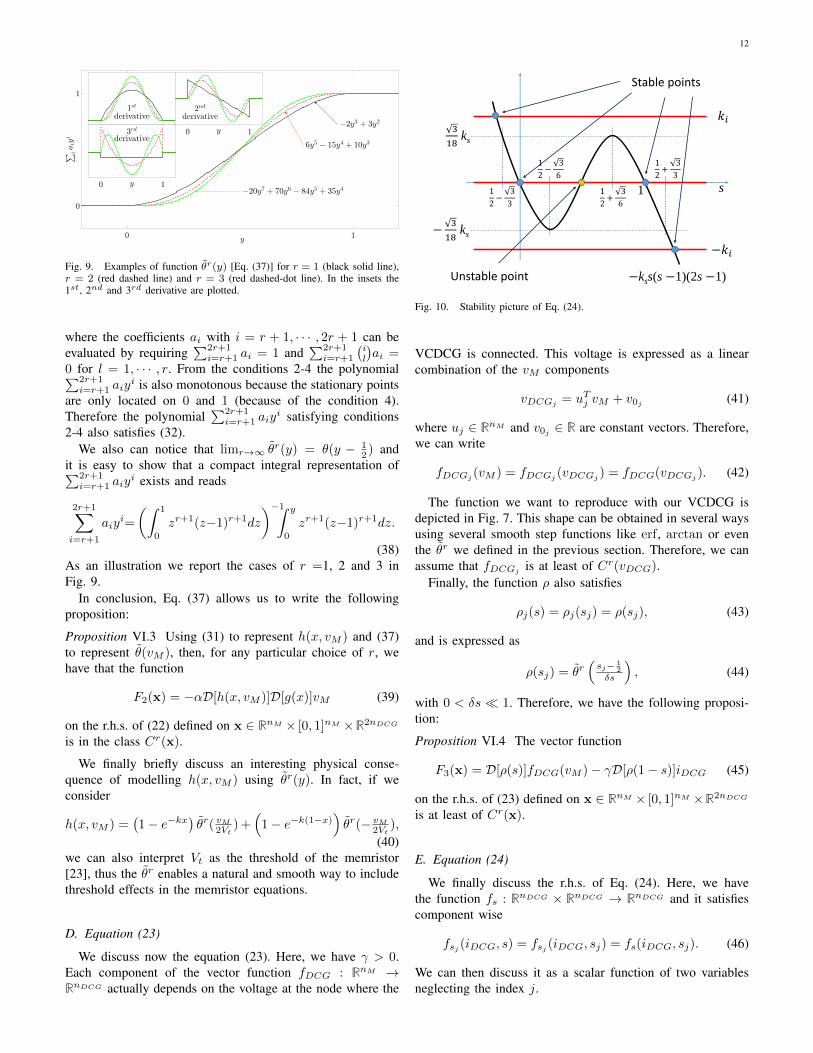
Fig. 9. Examples of function θr(y) [Eq. (37)] for r = 1 (black solid line),r = 2 (red dashed line) and r = 3 (red dashed-dot line). In the insets the1st, 2nd and 3rd derivative are plotted.
where the coefficients ai with i = r + 1, · · · , 2r + 1 can beevaluated by requiring
∑2r+1i=r+1 ai = 1 and
∑2r+1i=r+1
(il
)ai =
0 for l = 1, · · · , r. From the conditions 2-4 the polynomial∑2r+1i=r+1 aiy
i is also monotonous because the stationary pointsare only located on 0 and 1 (because of the condition 4).Therefore the polynomial
∑2r+1i=r+1 aiy
i satisfying conditions2-4 also satisfies (32).
We also can notice that limr→∞ θr(y) = θ(y − 12 ) and
it is easy to show that a compact integral representation of∑2r+1i=r+1 aiy
i exists and reads
2r+1∑i=r+1
aiyi=
(∫ 1
0
zr+1(z−1)r+1dz
)−1∫ y
0
zr+1(z−1)r+1dz.
(38)As an illustration we report the cases of r =1, 2 and 3 inFig. 9.
In conclusion, Eq. (37) allows us to write the followingproposition:
Proposition VI.3 Using (31) to represent h(x, vM ) and (37)to represent θ(vM ), then, for any particular choice of r, wehave that the function
F2(x) = −αD[h(x, vM )]D[g(x)]vM (39)
on the r.h.s. of (22) defined on x ∈ RnM × [0, 1]nM ×R2nDCG
is in the class Cr(x).
We finally briefly discuss an interesting physical conse-quence of modelling h(x, vM ) using θr(y). In fact, if weconsider
h(x, vM ) =(1− e−kx
)θr( vM2Vt ) +
(1− e−k(1−x)
)θr(− vM
2Vt),
(40)we can also interpret Vt as the threshold of the memristor[23], thus the θr enables a natural and smooth way to includethreshold effects in the memristor equations.
D. Equation (23)
We discuss now the equation (23). Here, we have γ > 0.Each component of the vector function fDCG : RnM →RnDCG actually depends on the voltage at the node where the
s
−kss(s −1)(2s −1)
1
3
18ks
−3
18ks
−𝑘𝑖
Stable points
Unstable point
1
2−
3
3
1
2−
3
6
1
2+
3
6
1
2+
3
3
𝑘𝑖
Fig. 10. Stability picture of Eq. (24).
VCDCG is connected. This voltage is expressed as a linearcombination of the vM components
vDCGj = uTj vM + v0j (41)
where uj ∈ RnM and v0j ∈ R are constant vectors. Therefore,we can write
fDCGj (vM ) = fDCGj (vDCGj ) = fDCG(vDCGj ). (42)
The function we want to reproduce with our VCDCG isdepicted in Fig. 7. This shape can be obtained in several waysusing several smooth step functions like erf , arctan or eventhe θr we defined in the previous section. Therefore, we canassume that fDCGj is at least of Cr(vDCG).
Finally, the function ρ also satisfies
ρj(s) = ρj(sj) = ρ(sj), (43)
and is expressed as
ρ(sj) = θr(sj− 1
2
δs
), (44)
with 0 < δs � 1. Therefore, we have the following proposi-tion:
Proposition VI.4 The vector function
F3(x) = D[ρ(s)]fDCG(vM )− γD[ρ(1− s)]iDCG (45)
on the r.h.s. of (23) defined on x ∈ RnM × [0, 1]nM ×R2nDCG
is at least of Cr(x).
E. Equation (24)
We finally discuss the r.h.s. of Eq. (24). Here, we havethe function fs : RnDCG × RnDCG → RnDCG and it satisfiescomponent wise
fsj (iDCG, s) = fsj (iDCG, sj) = fs(iDCG, sj). (46)
We can then discuss it as a scalar function of two variablesneglecting the index j.

13
The function fs(iDCG, s) is
fs(iDCG, s) = −kss(s− 1)(2s− 1)+
ki
1−∏j
θ
(i2min−i
2DCGj
δi
)−∏j
θ
(i2max−i
2DCGj
δi
)(47)
with ks, ki, δi, imin, imax > 0 and imin < imax. Note thatwhen ki = 0 Eq. (47) represents a bistable system. To under-stand the role of the variable s we notice that, by consideringonly the term in s in (47), it represents the bistable system withtwo stable equilibrium points in s = 0, 1 and an unstable equi-librium in s = 1
2 . Now, we consider again the terms in iDCGand δi� imin. In this case,
∏j θ((i
2min − i2DCGj )/δi) = 0 if
at least one iDCGj satisfies |iDCGj | > imin + δi/2 ≈ imin,otherwise the product is 1. On the other hand, we have∏j θ((i
2max − i2DCGj )/δi) = 0 if at least one iDCGj satisfies
|iDCGj | > imax + δi/2 ≈ imax, otherwise the product is 1.Therefore, if we consider ki >
√3/18ks, we have the stability
picture described in Fig. 10 where
• the red line located at ki represents terms in iDCG of(47) for the case in which at least one iDCGj satisfies|iDCGj | > imax. Therefore, we have only one stableequilibrium.
• The red line located at 0 is for the case in which at leastone iDCGj satisfies |iDCGj | > imin and all iDCGj satisfy|iDCGj | < imax. Therefore, we have two possible stableequilibria and an unstable one.
• The red line located at −ki is for the case in which alliDCGj satisfy |iDCGj | < imin. Therefore, we have onlyone stable equilibrium.
This picture can be summarized as follows: if at least one|iDCGj | > |imax| then the variable s will approach the uniquestable point for s < 1
2 −√33 < 0, while if all |iDCGj | <
|iDCGmin| the variable s will approach the unique stable point
for s > 12 +
√33 > 1. If at least one |iDCGj | > imin and all
|iDCGj | < imax then s will be either 12 −
√33 < s < 1
2 −√36
or 12 +
√36 < s < 1
2 +√33 .
Now, from Eq. (23) and the definition (44) we have that,if the at least one |iDCGj | > |imax|, then s < 0, ρ(s) = 0and ρ(1− s) = 1 and the equation (23) reduces to d
dt iDCG =−γiDCG. Therefore, the currents in iDCG decrease.
When all of them reach a value |iDCGj | < |imin| then sjumps and reaches the stable point s < 1 and we have ρ(s) = 1and ρ(1 − s) = 0 and the Eq. (23) reduces to d
dt iDCG =fDCG(vM ) (which is the simplified version (20) discussed inSec. V-D). Since fDCG(vM ) is bounded, the current iDCG isbounded and, if ks � max(|fDCG(vM )|), we have
sup(|iDCG|) ' |imax|. (48)
Therefore, using the analysis in this section we can concludewith the following proposition:
Proposition VI.5 The vector function
F4(x) = −kss(s− 1)(2s− 1)+
ki
1−∏j
θ
(i2min−i
2DCGj
δi
)−∏j
θ
(i2max−i
2DCGj
δi
)(49)
on the r.h.s. of (23) defined on x ∈ RnM × [0, 1]nM ×R2nDCG
is at least of Cr(x). Moreover, there exist imax, smax < ∞and smin > −∞ such that the variables s and iDCG can be re-stricted to [−imax, imax]nDCG × [smin, smax]nDCG ⊂ R2nDCG .In particular, smax is the unique zero of F4(s, iDCG = 0). Thissubset is invariant under the flow φiDCG,st of the dynamicalsystem (25) restricted to the variable iDCG and s only. More-over, the boundary points are limit points and for any openball of B ⊂ [−imax, imax]nDCG × [smin, smax]nDCG we havethat φiDCG,st (B) ⊂ [−imax, imax]nDCG × [smin, smax]nDCG isan open ball.
We can conclude this section with the last proposition thatcan be easily proven by using (28) and the proposition VI.5:
Proposition VI.6 If the variables x ∈ [0, 1]nM , iDCG ∈[−imax, imax]nDCG and s ∈ [smin, smax]nDCG then there existvmax <∞ and vmin > −∞ such that [vmin, vmax]nM ⊂ RnM
is an invariant subset under the flow φvMt of the dynamicalsystem (25) restricted to the variable vM only.
F. Existence of a global attractor
In the previous sections we have presented the equationsthat govern the dynamics of our SOLCs. We are now readyto perform the stability analysis of the SOLCs.
We consider our system given by (21)-(24), or in compactform by (25). The terminology we will use here follows theone in Ref. [4], in particular in Chapter 3. For our dynamicalsystem (25) we can formally define the semigroup T (t) suchthat T (t)x = x +
∫ t0F (T (t′)x)dt′, or defining x(t) = T (t)x
we have the more familiar
T (t)x(0) = x(0) +
∫ t
0
F (x(t′))dt′. (50)
Since we have proven in the previous sections that F (x) ∈Cr(X) with X the complete and compact metric spaceX = [vmin, vmax]nM × [0, 1]nM × [−imax, imax]nDCG ×[smin, smax]nDCG , then T (t) is a Cr-semigroup.
We recall now that a Cr-semigroup is asymptotically smoothif, for any nonempty, closed, bounded set B ⊂ X for whichT (t)B ⊂ B, there is a compact set J ⊂ B such that Jattracts B [4]. Here, the term ”attract” is formally definedas: a set B ⊂ X is said to attract a set C ⊂ X under T (t) ifdist(T (t)C,B)→ 0 as t→∞ [4].
Moreover, we have that a semigroup T (t) is said to be pointdissipative (compact dissipative) (locally compact dissipative)(bounded dissipative) if there is a bounded set B ⊂ Xthat attracts each point of X (each compact set of X) (aneighborhood of each compact set of X) (each bounded setof X) under T (t) [4]. If T (t) is point, compact, locally,dissipative and bounded dissipative we simply say that T (t) isdissipative. Now we are ready to prove the following lemmas:
14
Lemma VI.7 The Cr-semigroup T (t) defined in (50) isasymptotically smooth.
Proof: In order to prove this lemma we first need todecompose T (t) as the sum T (t) = S(t) + U(t). We takeinitially S(t) and U(t) as
U(t)x(0) =vM (0)− kDCGU+iDCG + U+v0 +
∫ t0F1(x(t′))dt′
x(0) +∫ t0F2(x(t′))dt′
00
(51)
S(t)x(0) =
kDCGU+iDCG − U+v0
0
iDCG(0) +∫ t0F3(x(t′))dt′
s(0) +∫ t0F4(x(t′))dt′
(52)
where kDCG > 0, v0 is the the constant vector whosecomponents are the v0j in (41), and U+ is the pseudoinverseof the matrix U whose rows are the vectors uTj in (41). It isworth noticing that for a well defined SOLC it is easy to showthat UU+ = I (the inverse, i.e. U+U = I , does not generallyhold).
We also perform two variable shifts:
vM → vM + U+v0 (53)s→ s− smax (54)
Since they are just shifts they do not formally change any-thing in Eqs. (51) and (52), except for additive terms inU+v0 and smax. Also, the metric space changes accordinglyto X → [vmin + U+v0, vmax + U+v0]nM × [0, 1]nM ×[−imax, imax]nDCG×[smin−smax, 0]nDCG . To avoid increasingthe burden of notation, in the following we will refer to allvariables and operators with the same previous symbols, whilekeeping in mind the changes (53) and (54).
Now, by definition, U(t) : X → [vmin + U+v0, vmax +U+v0]nM × [0, 1]nM × [0, 0]nDCG × [−smax,−smax]nDCG andit is easy to show that it is equivalent to the system
Cd
dtvM = (Av +BvD[g(x)])(vM − U+v0) + b (55)
d
dtx = −αD[h(x, vM )]D[g(x)](vM − U+v0) (56)
iDCG = 0 (57)s = −smax. (58)
By construction, from Eq. (28) and the definition ofh(x, vM ) in (40), U(t) represents a globally passive circuit.It is then asymptotically smooth, completely continuous1,and since it is defined in a compact metric space X , it isdissipative.
Now, following the lemma 3.2.3 of [4] we only need toprove that there is a continuous function k : R+ → R+ such
1A semigroup T (t), t > 0, is said to be conditionally completelycontinuous for t ≥ t1 if, for each t ≥ t1 and each bounded set B in Xfor which {T (s)B, 0 ≤ s ≤ t} is bounded, we have T (t)B precompact.A semigroup T (t), t ≥ 0, is completely continuous if it is conditionallycompletely continuous and, for each t ≥ 0, the set {T (s)B, 0 ≤ s ≤ t} isbounded if B is bounded [4].
that k(t, r) → 0 as t → ∞ and |S(t)x| < k(t, r) if |x| <r. In order to prove this statement, we first see that S(t) isequivalent to the system
vM = kDCGU+iDCG (59)x = 0 (60)d
dtiDCG = D[ρ(s+ smax)]fDCG(vM )+
− γD[ρ(1− s− smax)]iDCG (61)d
dts = fs(iDCG, s). (62)
Since vM = kDCGU+iDCG we have that fDCG(vM ) =fDCG(kDCGU+iDCG). From the definition and discussionon fDCG given in section VI-D, the variable change (41)and the definition of U+, we have that fDCGj (vM ) =fDCGj (vDCGj ) = fDCG(kDCGiDCGj ). Now, since we con-sider kDCG such that kDCGimax < vc/2, from the discussionin section VI-E and considering the variable change (54), theunique stable equilibrium point for S(t) is x = 0, and it isalso a global attractor in X . Moreover, this equilibrium ishyperbolic (see section VI-G), then there is a constant ξ > 0such that |S(t)x| < e−ξt. This concludes the proof.
Lemma VI.8 The Cr-semigroup T (t) defined in (50) is dis-sipative.
Proof: From lemma VI.7 T (t) is asymptotically smooth,then from the corollary 3.4.3 of [4] there is a compact setwhich attracts compact sets of X . There is also a compactset which attracts a neighborhood of each compact set of X .Therefore, since our X is bounded, the lemma follows.
At this point we recall some other definitions and resultsfrom topology of dynamical systems that can be found, e.g.,in Ref. [4] and will be useful for the next discussions.
For any set B ⊂ X , we define the ω-limit set ω(B) ofB as ω(B) =
⋂s≥0Cl
⋃t≥sT (t)B. A set J ⊂ X is said to
be invariant if, T (t)J = J for t ≥ 0. A compact invariantset J is said to be a maximal compact invariant set if everycompact invariant set of the semigroup T (t) belongs to J .An invariant set J is stable if for any neighborhood V of J ,there is a neighborhood V ′ ⊆ V of J such that T (t)V ′ ⊂ V ′for t ≥ 0. An invariant set J attracts points locally if thereis a neighborhood W of J such that J attracts points of W .The set J is asymptotically stable (a.s.) if J is stable andattracts points locally. The set J is uniformly asymptoticallystable (u.a.s.) if J is stable and attracts a neighborhood of J .An invariant set J is said to be a global attractor if J is amaximal compact invariant set which attracts each boundedset B ⊂ X . In particular, ω(B) is compact and belongs to Jand if J is u.a.s. then J =
⋃B ω(B).
Now, we are ready to prove the following theorem:
Theorem VI.9 The Cr-semigroup T (t) defined in (50) pos-sesses an u.a.s. global attractor A.
Proof: From the lemmas VI.7 and VI.8 we have that T (t)is asymptotically smooth and dissipative. Moreover, since Xis bounded, orbits of bounded sets are bounded and then thetheorem follows directly from the theorems 3.4.2 and 3.4.6 of[4].

15
G. Equilibrium points
With the previous lemmas and theorem we have provedthat T (t) has an u.a.s. global attractor. Roughly speakingthis means that, no matter the choice of initial conditionsx(0) ∈ X , T (t)x(0) will converge asymptotically to acompact bounded invariant set A. Since in our case X is acompact subset of R2nM+2nDCG , A can contain only equi-librium points, periodic orbits and strange attractors, and allof them are asymptotically stable [4]. We first show that thedynamics converge exponentially fast to the equilibria. We willthen argue about the absence of periodic orbits and strangeattractors.
First of all, it can be trivially seen from sections VI-D andVI-E that equilibria must satisfy uTj vM + v0j = −vc, 0, vc forany j. Moreover, as discussed in section V-D uTj vM +v0j = 0leads to unstable equilibria, while uTj vM +v0j = ±vc leads toasymptotically stable ones. However, these equilibria can bereached if the necessary condition
1
2+
√3
6< s < smax and |iDCGj | < |iDCGmax
| (63)
holds (see section VI-D and VI-E). It is also easy to see fromSecs. VI-D and VI-E that, by construction, this is a necessarycondition to have equilibrium points for T (t). However, thisdoes not guarantee that at equilibrium iDCG = 0.
For our purposes, we need to have iDCG = 0. In fact, atthe equilibria the SOLC has voltages at gate nodes that canbe only either −vc or vc. In such configuration of voltages,as discussed in section V-C, the gates can stay in correct ornon-correct configuration. In the former case no current flowsfrom gate terminals due to the DCMs and so the correspondentcomponent of iDCG must be 0 at the equilibrium. On the otherhand, if the gate configuration is not correct, at equilibrium wehave currents of the order of vc/Ron that flow from the gatesterminals (Sec. V-C). These currents can be compensated onlyby the components of iDCG. Therefore, if we indicate withKwrongvc/Ron the minimum absolute value of the currentflowing from the terminals of the gates when in the wrongconfiguration, Kwrong = O(1), and consider VCDCG with
iDCGmax < Kwrongvc/Ron, (64)
we have that the equilibria with nonzero components of iDCGdisappear and only equilibria for which iDCG = 0 survive.With this discussion we have then proven the followingtheorem
Theorem VI.10 If the condition (64) holds, the u.a.s. stableequilibria for T (t), if they exist, satisfy
iDCGj = 0 (65)sj = smax (66)
|uTj vM + v0j | = vc (67)
for any j = 1, · · · , nDCG. Moreover, this implies that the gaterelations are all satisfied at the same time.
This theorem is extremely important because it can berephrased in this way: T (t) has equilibria iff the CB problemimplemented in the SOLC has solutions for the given input.
We can analyze the equilibria even further. In fact we canprove their exponential convergence. With this aim in mind,we first analyze what happens to Eq. (22) when we are at anequilibrium. In this case, for each memristor we can have twopossible cases: vMj
= −Roff |iMj|, with |iMj
| the absolutevalue of the current flowing through the memristor and it isan integer > 1 times vc/Roff (this can be proven substitutingvalues of vo, v1 and v2 in equation (19) that satisfies the SO-gates and using coefficients of table I) and then xj = 1. In thesecond case we have vMj
= 0 and xj can take any value in therange [0, 1]. The latter case implies that the equilibrium is notunique for a given vM but we have a continuum of equilibria,all of them with the same vM , s and iDCG but different x. Theindetermination of some components of x (those related to thecomponents vM equal to 0) creates center manifolds aroundthe equilibria. However, these center manifolds are irrelevantto the equilibria stability since they are directly related toindetermination of the components of x and these componentscan take any value in their whole range [0, 1]. Therefore, wehave to consider only the stable manifolds of the equilibria.
In conclusion, since in the stable manifolds Cr semigroupswith r ≥ 1 have exponential convergence [9], and in our casethe center manifolds do not affect the convergence rate, thisproves the following theorem
Theorem VI.11 The equilibrium points of T (t) have exponen-tial convergence in all their attraction basin.
Finally, in order to check the scalability of SOLCs, we wantto study how the convergence of the equilibria depends on theirsize. We then write down the Jacobian of the system aroundan equilibrium point. Following the conditions in the theoremVI.10 and the equations discussed in the sections VI-B-VI-Eit can be shown that the Jacobian of F (x) of equation (25)evaluated in a equilibrium reads
JF (x = xs) =
∂F1
∂vM∂F1
∂x C−1Ai 0
0 ∂F2
∂x 0 0∂fDCG∂vM
0 0 0
0 0 0 ∂fs(iDCG,s)∂s
.
(68)We also assume that in the second block row we haveeliminated all equations for which vMj
= 0 holds, and fromthe second block column we have eliminated all columnsrelated to the indeterminate xj . This elimination is safe forour analysis since we want to study the eigenvalues of JF .In fact, we notice that the eigenvectors related to the non-nulleigenvalues are vectors with null components correspondingto the indeterminate xj since they are related to zero rows ofJF .
We can see from (68) that, since the last block column androw of JF have all zero blocks but the last one, the eigenvaluesof JF (x = xs) are simply the union of the eigenvalues of∂fs(iDCG,s)
∂s and the eigenvalues of
JFred(x = xs) =
∂F1
∂vM∂F1
∂x C−1Ai0 ∂F2
∂x 0∂fDCG∂vM
0 0
. (69)
Now, since ∂fs(iDCG,s)∂s is a diagonal matrix proportional to
16
the identity I , more explicitly ∂fs(iDCG,s)∂s = −ks(6s2max −
6smax + 1)I , its associated eigenvalues do not depend on thesize of the circuit.
In order to study the spectrum of JFred we notice that fromSec. VI-D we have ∂fDCG
∂vM= LDCGU where the derivative
is evaluated in either vDCGj = vc or −vc according to theequilibrium point. So, the eigenvalues of JFred are the timeconstants of an RLC memristive network.
While it is not easy to say something about the timeconstants of a general RLC network, in our case there aresome considerations that can be made. The capacitances,inductances, resistances are all equal (or very close to eachother if noise is added). Moreover, the network is ordered, inthe sense that there is a nontrivial periodicity and the numberof connection per node is bounded and independent of the size.From these considerations, our network can actually be studiedthrough its minimal cell, namely the minimal sub-networkthat is repeated to form the entire network we consider. Thisimplies that the slower time constant of the network is at mostthe number of cells in the network times the time constantof the single cell. This means that for polynomially growingSOLCs we have at most polynomially growing time constants.
H. On the absence of periodic orbits and strange attractors
In the previous sections we have proved that T (t) isendowed with an u.a.s. global attractor. We have also pro-vided an analysis of the equilibria proving their exponentialconvergence in the whole stable manifolds and discussed theirconvergence rate as a function of the size of the system,showing that this is at most polynomial. Therefore, in orderto have a complete picture of a DMM physically realizedwith SOLCs, the last feature should be discussed: what is thecomposition of the global attractor.
In order to analyze the global attractor we use a statisticalapproach. We make the following assumptions:
1) The capacitance C is small enough such that, if we per-turb a potential in a node of the network the perturbationis propagated in a time τC � τM (α) where τM (α) isthe switching time of the memristors (obviously linearfunctions of α). For our system the time constant τC isrelated to the memristance and C.
2) q of the function fDCG (see Fig. 7) is small enough suchthat the time τDCG(q) = iDCGmax
/q, satisfies γ−1 �τDCG, i.e., the the time that the current iDCG takes toreach iDCGmin
is much smaller than the time it takes toreach iDCGmax
.3) The switching time of the memristors satisfies γ−1 �
τM (α)� τDCG.4) The initial condition of x is taken randomly in X .Before proceeding we describe a peculiar behavior of our
SOLCs that can be proved by the nonlocality induced byKirchhoff’s current laws and looking at how the DCMs work.If we change a potential of order δV in a point of thenetwork ”quasi instantaneously”, namely within a switchingtime τC � τ � τM (α), there will be a sub-network S -including the point switched - that in a time of the order ofτC will change of the same order of δV many of the potentials
at the nodes. This change is simply the result of the RC natureof the network, the only component that survives at the timescale of τC . After a time of the order of τM (α), the sub-network S will reach a stable configuration as consequenceof the DCMs. Therefore, for a perturbation δV in a node ofthe circuit, there is, in a time τM (α), a reconfiguration of anentire region S of the network.
Now, from section VI-D and VI-E, we know that, if in agiven node j the current iDCGj reaches iDCGmax
the equationthat governs iDCG becomes d
dt iDCG = −γiDCG, so thecurrents decrease to imin in a time of the order of γ−1. Ifwe set imin very small compared to the characteristic currentsof the network, in a time of the order of γ−1 the potential atthe node j will experience a potential variation δV of the orderof Ronimax, if imax is large enough.
This last claim can be proved because, if the current imax
is of the order of Kwrongvc/Ron and satisfies (64), it meansthat the current from the network that compensates iDCGjcomes from some memristors that have been switched to Ron.Otherwise the current would be too small to reach valuesof the order of Kwrongvc/Ron. Therefore, for each VCDCGthat reaches imax a voltage variation of the order of Ronimax
is produced at the node where the VCDCG is connected.Morever, since τM (α)� τDCG, the network reconfigures theregion S before the current iDCGj starts increasing again.
With this in mind, and using the above conditions 1-4we can make a statistical interpretation of our network. Weconsider a system large enough and, since it is made of acombination of elementary cells, we assume that τC is smallenough such that the density of the nodes is uniform in thesubnetwork S. Taking as initial x(0) a random point in X ,we have that at the rate of τ−1DCG a fraction mDCG/nDCGof VCDCG reaches imax and consequently switches. Thismeans that there is a fraction of nodes that are kicked byδV ≈ Kwrongvc/Ron at a rate of τ−1DCG.
Following our discussion above, if x− is the configurationof the system before the kick, and x+ after (their temporaldistance is of the order of γ−1), then we have that the distancedist(x−,x+) is of the order of the radius of X defined asinfy∈X supx∈X dist(x,y). This means that these kicks bringthe system in points of X that are far from each other. Sincewe have chosen the initial x(0) random in X , also the kickswill take place randomly in time and in space (i.e., in thenetwork node). This means that the system explores the entireX . It is worth noticing that, like in the case of Monte Carlosimulations, when we estimate an integral in N dimensions[26], here the SOLC explores X in a way that is linear inthe number of variables, i.e., it needs a number of kicks thatgrows at most linearly with the dimension of the system.
All this analysis allows us to conclude that, in our SOLCs,periodic orbits or strange attractors cannot co-exist with equi-libria. In fact, both the periodic orbits and/or strange attractors,if they exist, produce large fluctuations of the potentials ofthe SOLC. These fluctuations are of the order of vc/Ronand are not localized but rather distributed in the entirenetwork, because of the combination of VCDCGs and DCMs.Therefore, from the previous analysis, if periodic orbits and/orstrange attractors exist they should force the system to explore

17
the entire space X . However, if an equilibrium point exists,then, by exploring X the system will intercept, within a timeof order τDCG times a number that grows only linearly withthe size of the system, the stable manifold of X and collapsesin the equilibrium point. Therefore, the global attractor is eiherformed by only equilibrium points or only by periodic orbitsand/or strange attractors.
I. Polynomial energy expenditure
We finally note that the SOLCs grow polynomially withthe input size, each node of each gate can support only finitevoltages (cut-off by the capacitances C) and at the equilibriumthe voltages do not depend on the size of the system. Thecurrents are also limited and their bounds are independent ofthe size of the SOLCs. The solution is found in a finite timewhich is polynomially dependent on the size of the SOLCs.Therefore, the energy expenditure can only grow polynomiallywith the SOLC size.
This can be also seen in a more mathematical way asfollows. Since the metric space X is a bounded compact space,the boundaries projected on each dimension subspace do notdepend on the SOLC size. Since the time is polynomiallydependent on the size of the SOLC, the energy expenditurecan only grow polynomially with SOLC size.
We now provide numerical evidence of all these statementsby solving two different NP problems, one hard.
VII. NP PROBLEMS SOLUTION WITH DMMS
In this section we discuss two different SOLCs for thesolution of two famous NP problems: the prime number fac-torization and the NP-hard version of the subset-sum problem.We show how, using the SO gates defined in Sec. V-C, andappropriate SOLCs, they can be solved with only polynomialresources.
A. Prime Factorization
Let us consider an integer n = pq where p and q aretwo prime numbers. Moreover, we define pj , qj , and nj thebinary coefficients of p, q and n such that p =
∑npj=0 pj2
j
and similarly for q and n. Therefore, np, nq and nn are thenumber of bits of p, q, and n respectively. The NP problemconsists in finding the two unique primes p and q such thatn = pq.
In order to find p and q we can write the product oftwo numbers expressed in binary basis using a closed set ofboolean functions. So we can express the product as f(y) = bwhere b is the collection of the coefficients nj , and y is thecollection of the pj and qj . It is easy to prove that f is notunique, but for our purposes this is not relevant.
According to our problem classification in Sec. II thefactorization problem belongs to the class CB, and we showhere that it belongs also to MPIM. In fact, starting from thef(y) = b we can build the SOLC as reported in figure 11for nn = 6. The inputs of the SOLC are the generatorsindicated by the nj . These generators impose voltages vc or−vc according to the logical value of nj . Therefore, this setof generators is the control unit of the DMM and encodes b.
qp0
qp1 + (qp0 − n0)/2
n0
n1
n2n3n4
n5
q2 q1 q0
qp2 + (qp1 + (qp0 − n0)/2− n1)/2
VCDCG
3 bit adder
p0
p1
p2
2 bit adder
Fig. 11. SOLC for solving a 6-bit factorization problem. The circuit iscomposed of the SOLGs described in section V.
The lines at the same potential indicated by pj and qj arethe output of our problem, i.e., they encode - through thevoltages - the coefficients pj and qj (namely y). In order toread the output of the SOLC it is thus sufficient to measurethe potentials at these lines. It is worth noticing that, once thegates have self-organized, the values of the potentials at allthe lines will be either vc or −vc. Therefore, there is no issuewith precision in reading the output, implying robustness andscalability of the circuit. In Fig. 11 the ”intermediate steps”of SOLC implementation are indicated for the reader who isnot familiar with boolean circuits.
Scalability analysis - It is clear that the circuit in Fig. 11 canbe built for any size of b and the number of SOLGs grows asn2n, so the SOLGs scale quadratically with the input. From theanalysis in the previous sections, the equilibria of this SOLCare the solutions of the factorization problem and they canbe exponentially reached in a time at most polynomial in nn.Finally, since the energy of this circuit depends linearly on thetime it takes to find the the equilibrium and on the number ofgates, also the energy is bounded. We thus conclude that suchcircuits will solve factorization with polynomial resources ifimplemented in hardware.
On the other hand, to simulate this circuit. i.e., to solvethe ODE (25), we need a bounded small time increment dtindependent of the size of the circuit, and dependent only onthe fastest time constant that can be associated to the timescales discussed in Sec. VI-H. Therefore, if a solution exists tothe prime factorization, and the SOLC fulfills the requirementsof Sec. IV-E, the problem belongs to the class MPIM. Moredetails on the complexity of this problem are discussed insection VIII.
It is worth noticing that the problem has no solution withinthis SOLC if either n is already a prime, or at least one of npor nq used to build the SOLC is smaller than the actual length

18
Fig. 12. Voltages at the nodes of the SOLCs for the prime factorization asa function of time (in arbitrary units). The circuits simulated are reported onthe right of each plot. They share the same topology as the one in Fig. 11.The solution is found when all voltages are either 1 or -1 (logical 1 and 0,respectively).
Fig. 13. Voltages at the nodes of the SOLCs for the prime factorizationas function of time (in arbitrary units). The circuits simulated is the 6-bitreported on the far bottom right of the plot. The input of the circuit is theprime 47.
of p or q used to solve the factorization problem2. This lastscenario can always be avoided by simply choosing np = nn−1 and nq = bnn/2c (or the reverse), where b·c stands for thefloor operator, i.e., it rounds the argument to the nearest integertowards minus infinity. This choice also guarantees that, if thep and q are primes, the solution is unique, and the trivialsolution n = n× 1 is forbidden.
We have implemented the circuit into the NOSTOS (NOn-linear circuit and SysTem Orbit Stability) simulator [27]–[31]developed by one of us (FLT). For the sake of simplicity, wehave implemented SOLCs with np = nq with length at most ofnn = np +nq . In this case, because of symmetry the possiblesolutions are two.
Numerical simulations - In Fig. 12 we present numericalresults for several nn. The simulations are performed bystarting from a random configuration of the memristor internalvariable x and switching on gradually the generators. Althoughnot necessary, we used a switching time for the generatorswhich is quadratic in nn. The plots report the voltages at theterminals of all the gates. Since we choose vc = 1, it can beseen that after a transient, all terminals approach ±vc, whichare the logical 1 and 0. When, thanks to the DCMs, all ofthem converge to ±vc, they are necessarily satisfying all gaterelations, and the SOLC has then found the solution.
We have performed hundreds of simulations using a 72-CPU cluster, and have not found a single case in which theSOLCs did not converge to the equilibria, thus reinforcing theanalysis in Sec. VI-H. It is also worth noticing that the largercase we dealt with (18-bit case) requires the simulate of adynamical system with approximatively 11,000 independentdynamic variables (i.e., vM , x, iDCG and s). We are thusdealing with an enormous phase space and yet we did not findanything other than equilibria. Clearly, this does not prove the
2If the integer n requires three or more primes to factorize, either the circuitneeds to be extended to include extra output numbers, or we let the circuitwith only p and q to break n into two integers (depending on the initialconditions). We can then proceed by reducing even further these numbers tillprimes are found.

19
TABLE IISIMULATION PARAMETERS
parameter value parameter value parameter valueRon 10−2 Roff 1 vc 1α 60 C 10−9 k ∞Vt 0 γ 60 q 10m0 −400 m1 400 imin 10−8
imax 20 ki 10−7 ks 10−7
δs 0 δi 0
c1
c2
c3
c1q1
c1q1 + c2q2
c1q1 + c2q2 + c3q3 s1 s0s3s4 s2
q3
q2
q1
Fig. 14. SOLC for solving a 3-number, 3-bit subset-sum problem. The circuitis composed of the SOLGs described in section V.
absence of strange attractors or limit cycles for all possiblesizes, but at least for the parameters we have used (see tableII) and the SOLC sizes we have tested this is the case.
Finally, in Fig. 13, we show the dynamics of the SOLCwhen we try to factorize a prime number. As expected, inthis case the trajectories never find an equilibrium. Since theSOLC has nonetheless a global attractor, what we are seeingin this plot could be either a complicated periodic orbit or astrange attractor.
B. The Subset-Sum Problem
We now show how to solve, with polynomial resources,within a SOLC the NP–hard version of the subset-sum problem(SSP), which is arguably one of the most important problemsin complexity theory [32]. The problem is defined as follows:if we consider a finite set G ⊂ Z of cardinality n, we wantto know whether there is a non-empty subset K ⊆ G whosesum is a given number s (NP-complete version). In addition,we will seek to find at least one subset (if it exists) thatsolves the problem (NP-hard version). The complexity of theSSP is formulated in terms of both its cardinality (n) and theminimum number of bits used to represent any element of G(namely the precision p). The problem becomes difficult tosolve when n and p are of the same order because the knownalgorithms to solve it are exponential in either n or p [3], [32].
We consider here the NP-hard version of the SSP in whichall elements of G are positive. The case in which they arenot can be equally implemented in the SOLCs but requires
Fig. 15. Voltages at the nodes of the SOLCs for the SSP in function of timein arbitrary units. The circuits simulated are reported on the right of each plot.
a slightly more complex topology and will be reported else-where. In order to solve the SSP we try to find the collectionof cj ∈ Z2 such that ∑
j
cjqj = s (70)
where qj ∈ G and j = 1, · · · , n. Therefore, our unknowns arethe cj , with y the collection of the cj . Equation (70) can bereadily represented in boolean form through a boolean systemf(y) = b where b is composed by the binary coefficientsof s padded with a number of zeros such that dim(b) equals

20
the minimum number of binary coefficients used to express∑j qj . It is easy to show that dim(b) ≤ log2(n−1)+p. This
boolean system can be implement in a SOLC as shown infigure 14. The control unit is here composed by the generatorsthat implement the binary coefficients of s and the output canbe read out by measuring the voltages at the lines pointed outby the cj in Fig. 14.
Scalability analysis - This circuit grows linearly in p andas n+log2(n−1) in n. The last term is due to the successiveremainders during the sum in (70). This is represented by theextra adders on the left of the SOLCs in Figs. 14 and 15.Also in this case, like the factorization, we have a SOLC thatgrows polynomially with both p and q so the SSP belongs tothe MPIM class (see Sec. II), indicating that, unlike the Turingparadigm, factorization and the subset-sum problem share thesame complexity within the memcomputing paradigm.
Numerical simulations - We have performed simulations ofthe SOLCs in a similar way as the factorization. The resultsare reported in figure 15. As in the case of the factorization,the solution is found when all gate voltages are either 1 or -1(logical 1 and 0, respectively). We have performed an extensiveanalysis of this case as well and up to n = 9 and p = 9 noperiodic orbits or strange attractors have been found by startingfrom random initial conditions. Finally, also for the subset-sumproblem, if no solution exists the system will not converge toany equilibrium.
VIII. DISCUSSION ON THE NP=P PROBLEM
In this work we have introduced and proved many state-ments derived from the new concept of Memcomputing Ma-chines, and in particular the easily scalable subclass we havenamed Digital Memcomputing Machines, and their abilityto solve complex problems with polynomial resources, ifimplemented in hardware. We have also shown in Sec. VIInumerical simulations of these machines that scale polynomi-ally with input size, which provides strong evidence that NPis equal to P. In this section we discuss this point and thelimitations to prove this statement formally.
The resources used to simulate DMMs and, in particular,SOLCs can be quantified in the number of floating pointoperations the CPU does to simulate them. Since we areactually integrating an ODE, x = F (x), (Eq. (25)), the numberof floating point operations depends i) linearly (if we use aforward integration method like the forward Euler or Runge-Kutta [33]) or at most quadratically (if we use a backwardmethod like backward Euler or Trapezoidal rule [33]) indim(x), and ii) depends on the minimum time increment weuse to integrate with respect to the total period of simulation,or in other words depends linearly on the number of time stepsNt. We discuss them separately.
We have seen in Sec. VII that for NP problems we have thatthe dim(x) scales polynomially in the input of the problem(quadratically in the number of bits for the factorization, andlinearly in both the precision and the cardinality of the setG for the SSP). Note also that we solve these NP problemsby mapping them into a more general NP-complete problem,the Boolean satisfiability (SAT) problem [32] and then we
build the SOLCs by encoding directly the SAT representingthe specific problem (this SAT is in compact boolean formthat we indicate with f(y) = b). This means that the dim(x)depends linearly on the number of elementary logic gates (i.e.,AND, OR, XOR) used to represent the SAT.
The number of time steps, Nt, to perform the simulationshas a double bound. The first one depends on the minimumtime increment ∆t, and the second on the minimum periodof simulation Ts. As discussed in VII-A, the former dependson the smallest time constant of the SOLC. Ultimately, thistime constant does not depend on the size of the circuit, buton the nature of the single devices we are simulating. On theother hand, Ts can depend on the size of the system. In fact,it is the minimum time we need to clearly find the equilibriaof the system. It is thus related to the largest time constant ofthe system. However, in section VI we proved that Ts growsat most polynomially with the size of the problem.
From all this, one can then infer that we can simulate poly-nomially a DMM using a Turing machine, suggesting NP =P. Recall, though, that we only gave theoretical and numericalarguments that, if equilibria exist, the global attractor does notsupport periodic orbits and/or strange attractors. We could not,however, come up with a formal proof of this last statement. Inother words, although we have strong evidence that this couldbe the case, as discussed in Sec. VI-H, and shown numericallyin Sec. VII, a rigorous formal proof is still lacking and wecannot settle the question of whether NP = P. (Note that itwould be enough to show that the basin of attraction satisfiesthe statistical conditions discussed in section IV-E.)
IX. CONCLUSIONS
With this paper we have shown how to employ digital(hence scalable) memcomputing machines - that use memoryto store and process information - to solve prime factorizationand NP-hard problems using polynomial resources. We haveproposed a practical implementation based on the concept ofself-organizable logic gates and circuits that can solve booleanproblems by self-organizing into their solution. We have usedtools of functional analysis to rigorously prove the requirementof polynomial resources with input size of these circuits, eventhough we could not still formally prove that NP=P.
These machines are not just a theoretical concept. Theycan be fabricated either with circuit elements with memory(such as memristors) and/or standard MOS technology. Theydo not require cryogenic temperatures or maintain quantumcoherence for a long time to work since they are essentiallyclassical objects, and map integers into integers. Therefore,they are quite robust to noise like our present digital Turingmachines implemented within the von Neumann architecture.
There are several directions that one can take from here,both from the experimental and theoretical point of view.Experimentally, it would be of course desirable to build thesemachines in the lab. However, at this juncture, the choice ofmaterials that would best fit their possible integration seems tosuggest an implementation using only MOS technology, ratherthan a combination of MOS devices and, e.g., memristors. ByMOS technology we do not mean here the use of transistors

21
in their switch mode only. Instead, we envision emulatorsof memristors that would perform the functions we havedescribed in this paper.
From the theory side, one is immediately drawn to considernew encryption protocols against these machines, in view ofthe fact that they can solve NP-hard problems in polynomialtime. Encryption schemes not based on the existing complexitytheory may be the way to proceed, but the options at this pointare wide open.
On a more speculative and possibly just academic scenario,we conclude by noting that one could extend the conceptof DMMs to topological vector spaces, in particular Hilbertspaces, thus allowing an extension of our concepts to quantumsystems. There is indeed some recent interest in fundamentalmemory elements such as superconducting memristors [34]and quantum memristive elements [35] that take advantageof quantum phenomena. A combination of such elements incircuits with the appropriate topology may allow the solutionof even more complex problems (e.g., super-exponential ones)in polynomial time.
Irrespective, the machines we propose are a realistic alterna-tive to Turing machines and could find applications in a widevariety of fields, such as machine learning, robotics, real-timecomputing, etc.
X. ACKNOWLEDGMENTS
We thank Hava Siegelmann, Fabrizio Bonani, and BjornTackmann for useful discussions. This work has been partiallysupported by the Center for Magnetic Recording Research atUCSD.
REFERENCES
[1] F. L. Traversa and M. Di Ventra, “Universal memcomputing machines,”IEEE Trans. Neural Netw. Learn. Syst., 2015.
[2] M. Di Ventra and Y. V. Pershin, “The parallel approach,” Nature Physics,vol. 9, p. 200, 2013.
[3] F. L. Traversa, C. Ramella, F. Bonani, and M. Di Ventra, “Mem-computing NP-complete problems in polynomial time using polyno-mial resources and collective states,” Science Advances, vol. 1, no. 6,p. e1500031, 2015.
[4] J. Hale, Asymptotic Behavior of Dissipative Systems, vol. 25 of Mathe-matical Surveys and Monographs. Providence, Rhode Island: AmericanMathematical Society, 2nd ed., 2010.
[5] R. Rivest, A. Shamir, and L. Adleman, “A method for obtaining digitalsignatures and public-key cryptosystems,” Communications of the ACM,vol. 21, pp. 120–126, 1978.
[6] O. Goldreich, Foundations of cryptography. Cambridge University Press,2001.
[7] H. T. Siegelmann, Neural networks and analog computation: beyond theTuring limit. Springer, 1999.
[8] H. Siegelmann, A. Ben-Hur, and S. Fishman, “Computational complex-ity for continuous time dynamics,” Physical Review Letters, vol. 83,p. 1463, 1999.
[9] L. Perko, Differential equations and dynamical systems, vol. 7. SpringerScience & Business Media, 3nd ed., 2001.
[10] F. L. Traversa and M. Di Ventra, “On the computational power ofmemcomputing machines,” Proc. of 15th international conference onnanotechnology (NANO 2015), 2015.
[11] D. Kozen, “On parallelism in turing machines,” in Foundations ofComputer Science, 1976., 17th Annual Symposium on, pp. 89–97, Oct1976.
[12] S. Fortune and J. Wyllie, “Parallelism in random access machines,”in Proceedings of the Tenth Annual ACM Symposium on Theory ofComputing, STOC ’78, (New York, NY, USA), pp. 114–118, ACM,1978.
[13] S. Wolfram, “Computation theory of cellular automata,” Communica-tions in Mathematical Physics, vol. 96, no. 1, pp. 15–57, 1984.
[14] J. Wiedermann, Parallel Turing machines. Department of ComputerScience, University of Utrecht, The Netherlands, 1984.
[15] R. M. Karp, “A survey of parallel algorithms for shared-memorymachines,” tech. rep., Berkeley, CA, USA, 1988.
[16] T. Worsch, “On parallel turing machines with multi-head control units,”Parallel Computing, vol. 23, no. 11, pp. 1683–1697, 1997.
[17] T. Worsch, “Parallel turing machines with one-head control units andcellular automata,” Theoretical Computer Science, vol. 217, no. 1, pp. 3–30, 1999.
[18] T. Worsch, “Cellular automata as models of parallel computation,” inComputational Complexity (R. A. Meyers, ed.), pp. 298–311, SpringerNew York, 2012.
[19] L. Landau and E. Lifshitz, Statistical Physics. Elsevier Science, 2013.[20] M. Di Ventra, Y. Pershin, and L. Chua, “Circuit elements with memory:
Memristors, memcapacitors, and meminductors,” Proceedings of theIEEE, vol. 97, pp. 1717–1724, Oct 2009.
[21] D. B. Strukov, G. S. Snider, D. R. Stewart, and R. S. Williams, “Themissing memristor found,” Nature, vol. 453, pp. 80–83, May 2008.
[22] F. Bonani, F. Cappelluti, S. D. Guerrieri, and F. L. Traversa, WileyEncyclopedia of Electrical and Electronics Engineering, ch. HarmonicBalance Simulation and Analysis. John Wiley and Sons, Inc., 2014.
[23] M. Di Ventra and Y. V. Pershin, “On the physical properties of mem-ristive, memcapacitive and meminductive systems,” Nanotechnology,vol. 24, p. 255201, 2013.
[24] Y. V. Pershin and M. Di Ventra, “Memory effects in complex materialsand nanoscale systems,” Adv. Phys., vol. 60, pp. 145–227, 2011.
[25] K. Eshraghian, O. Kavehei, K.-R. Cho, J. Chappell, A. Iqbal, S. Al-Sarawi, and D. Abbott, “Memristive device fundamentals and modeling:Applications to circuits and systems simulation,” Proceedings of theIEEE, vol. 100, no. 6, pp. 1991–2007, 2012.
[26] F. Rossi, Theory of Semiconductor Quantum Devices, MacroscopicModeling and Simulation Strategies. Berlin: Springer-Verlag, 2016.
[27] F. L. Traversa and F. Bonani, “Improved harmonic balance implementa-tion of floquet analysis for nonlinear circuit simulation,” {AEU} - Inter.J. Elec. and Comm., vol. 66, no. 5, pp. 357 – 363, 2012.
[28] F. L. Traversa and F. Bonani, “Frequency-domain evaluation of theadjoint floquet eigenvectors for oscillator noise characterisation,” IETCirc. Device Syst., vol. 5, no. 1, pp. 46–51, 2011.
[29] F. L. Traversa and F. Bonani, “Selective determination of floquet quan-tities for the efficient assessment of limit cycle stability and oscillatornoise,” IEEE Trans. Comput.-Aided Design Integr. Circuits Syst, vol. 32,no. 2, pp. 313–317, 2013.
[30] F. L. Traversa, F. Bonani, Y. V. Pershin, and M. Di Ventra, “Dynamiccomputing random access memory,” Nanotechnology, vol. 25, p. 285201,2014.
[31] F. L. Traversa, Y. V. Pershin, and M. Di Ventra, “Memory models ofadaptive behavior,” IEEE Trans. Neural Netw. Learn. Syst., vol. 24,pp. 1437–1448, Sept 2013.
[32] M. R. Garey and D. S. Johnson, Computers and Intractability; A Guideto the Theory of NP-Completeness. New York, NY, USA: W. H. Freeman& Co., 1990.
[33] J. Stoer and R. Bulirsch, Introduction to numerical analysis. Springer-Verlag, 2002.
[34] S. Peotta and M. Di Ventra, “Superconducting memristors,” PhysicalReview Applied, vol. 2, p. 034011, 2014.
[35] P. Pfeiffer, I. L. Egusquiza, M. Di Ventra, M. Sanz, and E. Solano,“Quantum memristors,” arXiv:1511.02192, 2015.