Polyspherical Description Polyspherical Description ofof

a N-atom systema N-atom system

Christophe IungLSDSMS, UMR 5636

Université Montpellier IIe-mail : iung@univ-montp2.fr

Collaboration avec Dr. Fabien Gatti, Dr. Fabienne Ribeiro et G. Pasin

Pr. Claude Leforestier (Montpellier)Pr. Xavier Chapuisat et Pr. André Nauts

(Orsay et Louvain La Neuve)

H

F

FF

nCH

CF3H

Intramolecular Energy transfer in an excited System :

Dynamical Behaviour of anExcited system :

Is it ergodic or selective?

FIT of a Potential Energy Surface(PES) to describe the water solvent

(H2O)n

EXAMPLES OF SYSTEMSEXAMPLES OF SYSTEMS

1- Born-Oppenheimer Approximation :

===> The Potential energy surface V can be expressedin terms of (3N-6) internal coordinates that describe the deformation of the molecular system

2- A Body-Fixed Frame (BF) has to be defined :

Tc = Tc(G : 3 coordinates) + Tc(rotation-vibration:3N-3

coordinates)

Schrödinger ro-vibrational EquationSchrödinger ro-vibrational Equation

3- Ro-Vibrationnal Schrödinger Equation : an eigenvalue equation

H |> = (Tc+V) |) internal coordinates> = Ero-vibrationnal|

>

4- Definition of a working basis set in which the Hamiltonian is diagonalized, this basis should contain 150000 states, for instance.

2- Expression of the Kinetic Energy Operator (KEO) Tc

3- Calculation and Fit of the Potential energy Surface (PES), V, a function of the 3N-6 internal nuclear coordinates.

1- Choice of the set of coordinates adopted to describe the system : A crucial Choice

5- Schrödinger Equation to be solved

-Pertubative Methods (CVPT...)

- Variational method (VSCF, MCSCF, Lanczos,

Davidson,...)6- Comparison between the calculated and experimental spectrum

Problem to be SolvedProblem to be Solved

RectilinearLow energy spectrum

Very Simple Expression of the Kinetic Energy OperatorBasis of the traditional

Spectroscopy

Y1

Z1 Z2

Y2

CurvilinearLarge amplitude motions

More Intricate expression of the KEO

1-Choice of the set of coordinates1-Choice of the set of coordinates

* We need an exact expression of the KEO adapted to the numerical methods used to solve the Schrödinger equation.

* We have to know how to act this operator on vectors of the working basis set.

2- Expression of the KEO (Tc)

withP

ix = - i xi

,

3- Analytical Expression of the PES calculated on a grid (of few thousands

points). (Fit of this function)

Potential Energy Surface

Coordinates 2

Coordinate 1

1- KEO Expression 2.1 : Historical Expressions of the KEO 2.2 : More Recent (1990-2005) Strategies that provide

KEO operator

3- Direct Methods that solve the Schrödinger Equation

3.1 : Lanczos Method3.2 : Block Davidson Method

Outlines of the talkOutlines of the talk

2- Polyspherical Parametrization of a N-atom System (IJQC review paper on the web)

2.1 : Principle2.2 : Application to the study of large amplitude motion 2.3 : Application to highly excited semi-rigid systems : Jacobi Wilson Method

4- Application to HFCO

1- Some Famous References1- Some Famous References

B. Podolsky, Phys. Rev. 32,812 (1928)

E.C. Kemble “The fundamental Principles of Quantum Mechanics”Mc GrawHill, 1937

E.B. Wilson, J.C. Decius, P.C. Cross “Molecula Vibrations”McGrawHill, 1955

H.M. Pickett, J. Chem. Phys, 56, 1715 (1971)

A. Nauts et X. Chapuisat, Mol. Phys., 55, 1287 1985

N.C. Handy, Mol. Phys., 61, 207 (1987)

X.G. Wang, E.L. Sibert et M.S Child, Mol. Phys., 98, 317 (2000)

Quantum Expression of KEO for J=0 in Quantum Expression of KEO for J=0 in the Euclidean Normalizationthe Euclidean Normalization

2Tc = (tpx)+ px

where pxi is the conjugate momentum associated with the mass-ponderated coordinates

If a new set of curvilinear coordinates qi (i=1,…,3n-6) is introduced

where J is the matrix which relies the cartesian coordinates to the new set of coordinates qi

The determinant of J is the Jacobian of the transformation denoted by J

dEuclide = dx1 dx2… dx3N-6= J dq1 dq2… dq3N-6

q = J-1 x px=t(J-1) pq

TTcc expression of the KEO for J=0 expression of the KEO for J=0 in Euclidian normalizationin Euclidian normalization

If 2Tc = (tpx)+ px and px=t(J-1)pq

2Tc = (tpq)+ J-1 t(J-1) pq

2Tc = (tpq)+ g pq

det(g)=J-2

2Tc = J-1 tpq J g pq

What is the adjoint of pqi ? It depends on the normalisation chosen

In an Euclidean Normalization (pqi)+ = J-1 pqi J where J est the Jacobian

Démonstration de (pq)+=J-1 pq J en normalisation

euclidienne Définition de l’adjoint de pqi ?<(pqi)+| >= < | pqi >

Or ... pq (J dq1 dq2… dq3n-6

si (J s ’annule sur les bornes d ’intégration

... pq (J dq1 … ... pq (J dq1…dq3n-6... J pq

(dq1…dq3n-6

d ’où ... (J-1pq J Jdq1… dq3n-6 ... pq (Jdq1...

dq3n-6

... (J-1pq J dEuclide ... pq (dEuclide

d ’où (pq)+ = J-1 pq J

Let use the expression of the Laplacian in spherical coordinates :

2Tc = -h/2

This expression can be re-expressed by

Other way to find 2Tc = J-1 tpq J g pq

Jacobian the is where Jq

gJq

Jl

lk

k

n

lk

,

63

1,

1

2Tc = (tpq)+ g pq

This normalization can be helpful to calculate some integrals.

(Euclide)*ÂEuclideEuclidedEuclide (Wilson)*ÂWilsonWilsondWilson

(Euclide)*ÂEuclideEuclideJdq1 … dq3n-6 (Wilson)*ÂWilsonWilsondq1 … dq3n-6

(J0.5Eu)* (J0.5ÂEuJ-0.5)J0.5Eu)dWilson (Wilson)*ÂWilsonWilsondWilson

(Wilson)* ÂWilsonWilson

2TcW = J0.5Tc

EuJ-0.5 = J0.5J-1 tpq J g pq J-0.5J-0.5tpqJ g pq J-0.5

Quantum Expression of TQuantum Expression of Tcc for J=0 for J=0 in Wilson Normalization in Wilson Normalization dWilson =dq1 dq2… dq3n-6

2 TcWilson J-0.5 tpq J g pq J-0.5

Rectilinear Rectilinear DescriptionDescription

J, g do not depend on J, g do not depend on qq

2 TcWilson J-0.5 tpq J g pq J-0.5

OR

2TcEuclide

= J-1 tpq J g pq

Curvilinear Curvilinear DescriptionDescription

J, g depend on J, g depend on qq

2Tc =tpq g pq No problem for Tc

but problem for the fit of Vand for the

physical meaning of q

Problem of no-commutation More Intricate expression

To find and to act on a basisBut easy fit of V

et better physical meaning of q

Different strategies developed :Different strategies developed :Application of the Chain RuleApplication of the Chain Rule

Handy et coll. (Mol. Phys., 61, 207 (1987))Handy et coll. (Mol. Phys., 61, 207 (1987))

Starting with the expression with cartesean coordinates

: 2Tc = (tpx)+ px

The chain rule is acted (with the kelp of symbolic calculation)and provides :

2 Tc = gkl pk pl + hk pk in Euclidean Normalization

Other normailization can be used…But it results more intricate expression of the KEO Tc

N

i i

j

k x

qh

3

12

2

with

Other formulation :Other formulation :Pickett expression: JCP, 56,1715 (1972)Pickett expression: JCP, 56,1715 (1972)

lk

kl

klkkl

n

lk q

J

q

g

q

J

q

J

q

JgV

ln

4

1ln

4

1lnln

8

1'

2

263

1,

Starting from 2 TcWilson = J-0.5 tpq J g pq J-0.5

One can find

2 TcWilson = tpq g pq + V’

V’ « extrapotential term » that depends on the masses. It can be treated with the potential

This formulation has be exploited by E.L. Sibert et coll. in hisCVPT perturbative formulation: J. Chem. Phys., 90, 2672 (1989)

Ideal features of a KEO expressionIdeal features of a KEO expression

Compact Expression of the KEO : larger is the number of terms, larger is the CPU time

Use of a set of coordinates adapted to describe the motion of atomsin order

*to reduce the coupling between these coordinates

* to define a working basis set such that the Hamiltonian matrix is sparse

The numerical action of the KEO must be possible and not too much CPU time consuming

The expression should be general and should allow to treat a largevariety of systems

2- Polyspherical Parametrization

The N-atom system is parametrized by (N-1) vectors described by their Spherical Coordinates ((Ri,i, i), i=1,...,N-1)

The General Expression of the KEO is given in terms of either

1- the kinetic momenta associated to the vectors

And the (N-1) radial conjugate momenta pRi

===> adapted to the description of large amplitude motion

OR

2- the momenta conjugated with the polyspherical

coordinates ((Ri,i, i),i=1,...,N-1)

===> adapted to the description of highly excited semi-rigid systems

(pRi, p i

, p i)

= -i

Ri

Development of this parametrizationFirst description of its interest :

X. Chapuisat et C. Iung , Phys. Rev. A,45, 6217 (1992)

Review papers : F. Gatti et C. Iung,J. Theo. Comp. Chem.,2 ,507 (2003) et

C. Iung et F. Gatti, IJQC (sous presse)

Orthogonal Vectors : F. Gatti, C. Iung,X. Chapuisat JCP, 108, 8804 (1998), and 108, 8821 (1998)

M. Mladenovic, JCP, 112, 112 (2000)

NH3 Spectroscopy : F. Gatti et al , JCP, 111, 7236, (1999) and 111, 7236, (1999)

Non Orthogonal Vectors : C. Iung, F. Gatti, C. Munoz, PCCP, 1, 3377 (1999) M. Mladenovic, JCP, 112, 1082 (2000);113,10524(2000)Semi-Rigid Molecules : C. Leforestier, F. Ribeiro, C. Iung 114,2099 (2001) F. Gatti, C. Munoz and C.Iung : JCP, 114, 8821 (2001) X. Wang, E.L.Sibert and M. Child : Mol. Phys, 98, 317(2000)

H.G Yu, JCP,117, 2020 (2002);117,8190(2002)

HF trimer : L.S. Costa et D.C. Clary, JCP, 117,7512 (2002)Diatom-diatom collision : E.M. Goldfield,S.K. Gray, JCP, 117,1604(2002) S.Y. Lin and H. Guo, JCP, 117, 5183(2002)

““ORTHOGONAL” SET OF VECTORSORTHOGONAL” SET OF VECTORS

Polyspherical Coordinates :R3, R2, R1,

1,

et out-of-plane dihedral angle)

BF GzH H

Jacobi Vectors Radau Vectors

O OC C

F H

i i

i iPP

T

2

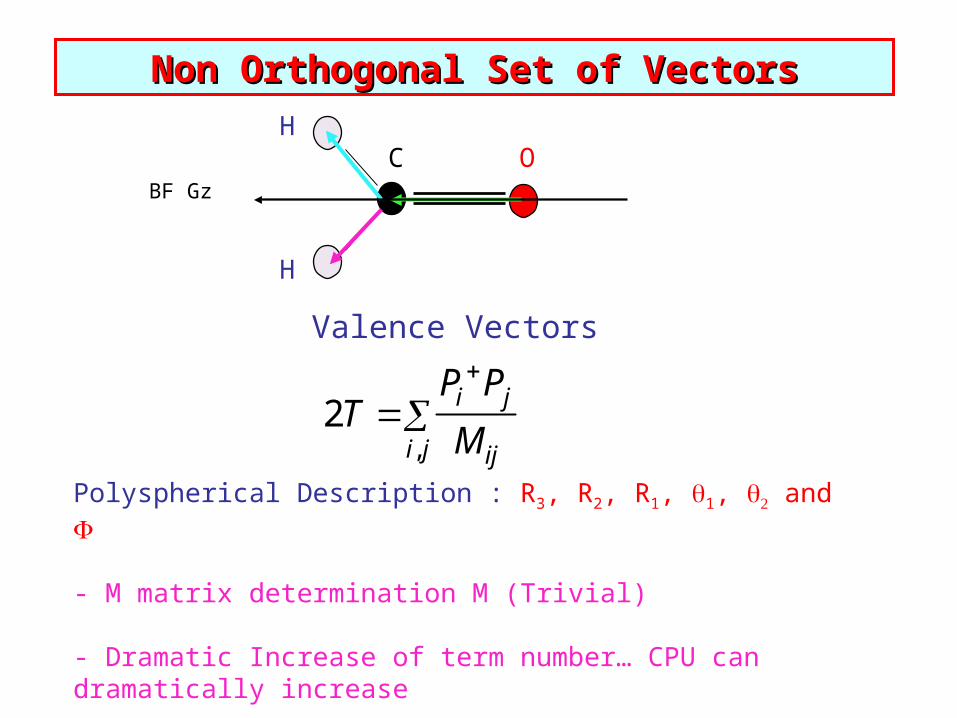
Non Orthogonal Set of VectorsNon Orthogonal Set of Vectors

Polyspherical Description : R3, R2, R1, 1, and

- M matrix determination M (Trivial) - Dramatic Increase of term number… CPU can dramatically increase

2T

P i

P jMiji, j

Valence Vectors

BF Gz

OCH

H

Determination de la Matrice MDetermination de la Matrice M

Any set of vectors can be related to a set of Jacobi vectors :

R A

r Jacobi M = At A

if 2T

(P i

Jac ) P i

Jac

ii

P i

P jMiji, j

La Matrice M est une matrice très facile à déterminer et dépendant des masses

Elle permet de généraliser les résultats obtenus avec les vecteurs orthogonaux

Developed expressions of the KEO

*kinetic momentum Li

associated with Ri and the radial momenta

*Conjugate radial and angularmomenta

(L i , P iR = - i

Ri

)

By using Obtained by the

substitution of the angular momentum

P i =

PiR R i

Ri

+

L i

R i

Ri2

* Lix - sin i pi cos i p

i

* Liy cos i pi sin i p

i

* Liz pi

A BF (Body Fixed) frame has to be defined to introduce the total angular momentum (full

rotation) vector J

{

by dsubstitute is ; from Starting ic PPMPT

2

P

iR = - i Ri

, Pi = -i

i

, Pi

= - i i

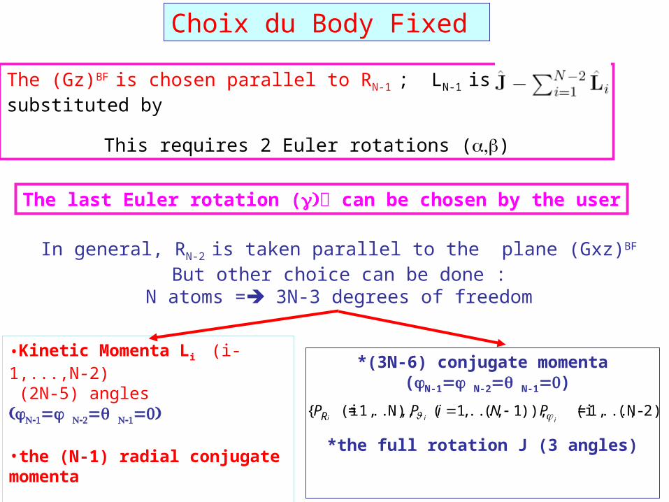
Choix du Body Fixed

The (Gz)BF is chosen parallel to RN-1 ; LN-1 is substituted by

This requires 2 Euler rotations ()

The last Euler rotation ( can be chosen by the user

In general, RN-2 is taken parallel to the plane (Gxz)BF

But other choice can be done :N atoms = 3N-3 degrees of freedom

•Kinetic Momenta Li (i-1,...,N-2) (2N-5) angles •the (N-1) radial conjugate momenta

• the full rotation J (3 angles)

*(3N-6) conjugate momenta (N-1N-2N-1)

*the full rotation J (3 angles)

{PiR (i = 1,..., N), P

i (i 1, ...,(N 1)), Pi (i = 1,..., (N - 2))

By taking into account the fact thatBy taking into account the fact thatRRN-1N-1 and R and RN-2 N-2 are linked to the BF frameare linked to the BF frame

(problem of no-commutation of the operator(problem of no-commutation of the operator that depends on vectors Rthat depends on vectors RN-1N-1 and R and RN-2 N-2 ))

It results in general expression of the KEOIt results in general expression of the KEO

with

One finds that :

The problem of no-commutation are such that

KEO developed expression for a system describedby a set of (N-1) orthogonal vectors

KEO developed expression for a system describedby a set of (N-1) orthogonal vectors

General Expression of TGeneral Expression of Tc c in terms of the conjugate momentain terms of the conjugate momentaAssociated with the polyspherical coordinates Associated with the polyspherical coordinates Expression used to study semi-rigid systemsExpression used to study semi-rigid systems

F. Gatti, C. Munoz, C. Iung, JCP, 114, 8821 (2001)F. Gatti, C. Munoz, C. Iung, JCP, 114, 8821 (2001)

The expression of the KEO are known…The expression of the KEO are known…How can we use them How can we use them

for instance for semi-rigids systems ?for instance for semi-rigids systems ?

1- Orthogonal Coordinates provides rather simple expression of KEO…

However, these coordinates does not necessary describe a real deformation of the system

2- Interesting coordinates, such valence coordinates, are not ‘orthogonal’ The KEO expression is intricate

Two sets of coordinates can be used…This is the idea of the Jacobi-Wilson Method

Definition of “Curvilinear Normal Coordinates”,Qi, In terms of polyspherical coordinates qj :

Hvib0

1

2(qnFn,m

n ,m

3N 6

qm pnGn ,m0 pm ) Gn ,m

0 G(qeq ) Fn,m 2V

qnqm

qeq

where and

QL 1qPolysphericalCoordinates

Normal ModesDefined in terms of

Polyspherical coordinates

Advantages : Simplicity of Tc in terms of polyspherical coordinates

Physical Interest of the Normal Modes

Jacobi-Wilson Method(C. Leforestier, A. Viel, C. Munoz, F. Gatti and C. Iung, JCP, 114, 2099 (2001))

Pq is substituted by (tL) PQ in Tc

JACOBI-WILSON STRATEGYJACOBI-WILSON STRATEGY

H

Jacobi Vector

OC

F

• Description Polyspherique

• Simple Expression of the KEO T JACOBI

• Normal Mode Coordinates :

• Definition of a working basis set :

WILSON

1...3N 6

qLQ 1

H H 0 V T

DIAGONALIZATION

Application to HFCO et H2CO Up to10000 cm-1

Improvement of the zero-order basis setImprovement of the zero-order basis set

On can take into account to the diagonal anharmonicity:

Hvib

0, 2

2

2

2Q V (Q )QQeq

H H 0 V T

m

N

mnmnmn

n

anharm

qGG

qT

VVV

)(2

63

,

0,,

2

H Matrix calculationH Matrix calculation

q

semi-analytical estimation of its action

VG

pseudo spectral scheme used

Spectral Representation :

Grid Representation:

(Q1...Q6 ) n1 ...n6n1

(n1...n6

Q1)...n6(Q6 )

(Q1a ...Q6 f ) n1 ...n6n1

(n1...n6

Q1a )...n6(Q6 f )

Ideal features of a method that provides Ideal features of a method that provides eigenstates and eigenvalues which can be locatedeigenstates and eigenvalues which can be located

in a dense part of the spectrumin a dense part of the spectrum

•Application to a large variety of systems ;

•Use of huge basis set ;

•Obtention of eigenvalues and eigenstates;

•Control of the accuracy of the results ;

•Small CPU time, Small memory requirement ;;

•Easy to use and to adopt ;

•Specific Calculation of energies in a given part of the spectrum ;

Iterative Construction of the Krylov subspace generated by {un, n=O,N} :

1- Initialization : A first guess vector u0 is chosen

2- Propagation : The following vector un+1 is calculated

n+1 un+1 = (H – n) un – n un-1

with

n = <un|H|un>

n+1= <un+1|H|un>

LANCZOS METHODLANCZOS METHOD

• Lanczos Method:

0

BNB

N

H

dimdim

0211

10

dim

LANCZOS FEATURESLANCZOS FEATURES

• Avoid the determination of the full H matrix.• The convergence is slower when the state density

increases

DIAGONALISATION DE HDIAGONALISATION DE H

Diagonalisationdirecte

Méthode de

Lanczos

Ouverture de Fenêtres en

énergie

E0

0

50

100

150

200

250

300

0 5000 10000 15000

Energies en cm-1

r (

po

ur

10

0 c

m-1

)

• Spectral Transform . Lanczos applied to G=(Eref°-H)-1. or exp(-(H-Eref)2)

One has to open some window energyOne has to open some window energy

Modified Block-Davidson AlgorithmModified Block-Davidson Algorithm to to calculate calculate

a set of a set of b coupled eigenstatesb coupled eigenstates

Method based on one parameter : Method based on one parameter : which sets the accuracy which sets the accuracyF. Ribeiro, C. Iung, C. Leforestier JCP in pressF. Ribeiro, C. Iung, C. Leforestier JCP in press

C. Iung and F. Ribeiro JCP in pressC. Iung and F. Ribeiro JCP in press

The working basis set Banh is divided into : Banh = P° Q .

Where P° contains the zero-order states which play a significant rôle in the calculation performed :

H is diagonalized in P°, et this new basis set {u°i ,E°i } is used during the Davidson scheme

E°1

E°i

Eanh1

Eanhq

0

0

0

0

0

0

P°

Q

H°H°==

Prediagonalization step in order to reducePrediagonalization step in order to reducethe off-diagonal termsthe off-diagonal terms

We can defined the block of states using the second-order perturbation

00002

,

EE

uHu

EE

uHu q

Qq q

q

States such that are retainedun a given block :

1.02,

Determination of the Block of statesDetermination of the Block of states

• Faible barrière de dissociation (14000 cm-1)

HFCO HF + CO

• Mode de déplacement hors du plan très découplé à haute énergie.

• Forte densité d ’états

APPLICATION TO HFC0APPLICATION TO HFC0

Selectivity of the energy transfer in HFCOwhose out-of-plane mode is excited

Moore et coll. have studied the highly excited out-of-plane overtones (nout-of-plane, n=14,…,20) :

they predict the localization of energy in these states

How can we understand that a highly excited state can be localized in one mode

while the state density is large for Eexc=14000-20000cm-

1?

6 modes

2981 cm-1 : CH stretch1837cm-1 : C=0 stretch1347 cm-1 : HCO bend1065 cm-1 : CF stretch662 cm-1 : FCO bend

1011 cm-1 Out of plane mode

In-plane modes

C

F

OH

Excitation of the Out-of-plane mode

• Between 1 and 60 Davidson iterations are required to calculate each state.E is not a correct indicator of the convergence

Davidson Iteration Number

-État 60-État 120-État 180

Lan

czo

s

CONVERGENCE OF THE DAVIDSON SCHEMECONVERGENCE OF THE DAVIDSON SCHEME

Nombre d ’itérations Davidson

ErrorOn theEnergy (cm-1)

• I : IIq(M)IImax < 10 cm-1

Pour E < 0.01 cm-1

IIq(M)IImax < 50 cm-1

Pour E < 0.5 cm-1

Convergence criterionConvergence criterion

Davidson Iteration Number

Err

eur

(cm

-1)

)()( )ˆ( Mr

MrM MM

HEq

• IIq(M)II constitue an excellentIndicator of the convergenceAnd the accuracy of the eigenenergy and eigenstate.

Numerical CostNumerical Cost

0

1000

2000

3000

4000

5000

6000

7000

8000

2000 2500 3000 3500 4000 4500 5000 5500 6000 6500

BLOC-DAVIDSON

LANCZOS

Nombre d ’actions de H

Energie d ’excitation (cm-1)

Determination of an Active Space specificaly Determination of an Active Space specificaly built to study a given statebuilt to study a given state

Example : state |106> in HFCO

(State n° 1774, in a 100,000 state primitive basis setCaracterized by vmax(in plane)=8 and Emax=32,000cm-1)

We begin with a Davidson calculation performedon |106>(0) in a 7,000 state basis set defined by vmax(in plane)=4 and Emax=24,000cm-1

The Davidson scheme in this small basis set converges andprovides an estimation of the eigenstate studied: |106>(1)

The largest |v1,…,v6>°contributions of this estimated eigenstate |106>(1) are retained

in a small (368 states) « active space » Po used in the calculation in the large (100,000 states) basis set

6 8 10Zero Order Energy 6439.6 8641.9 10849.9 P0 dimension

1 1 368 Prediagonalized Energy of the guess

6439.6 8641.9 10127.1 Converged Energy 6018.4 7984.9 9948.8 Overlap with the guess

0.77 0.64 0.92 Main Contributions of the eigenstate

+0.77 6 +0.28(

+ 0.64 8 0.30(

0.31 + 0.51 10

v1averaged 0.27 0.47 0.69

v2averaged 0.08 0.11 0.17

v3averaged 0.14 0.31 0.37

v4averaged 0.06 0.20 0.15

v5averaged 0.02 0.23 0.04

v6averaged 5.47 6.75 8.57

Application to the calculation of highly Application to the calculation of highly Excited overtones in HFCOExcited overtones in HFCOState 10State 1066: State n°1700: State n°1700

Similar coefficientsobtained for different

overtones :The nature of the

couplingis identical

for these overtones

The CH stretch is the more

coupled mode

CH stretch

HCO bend

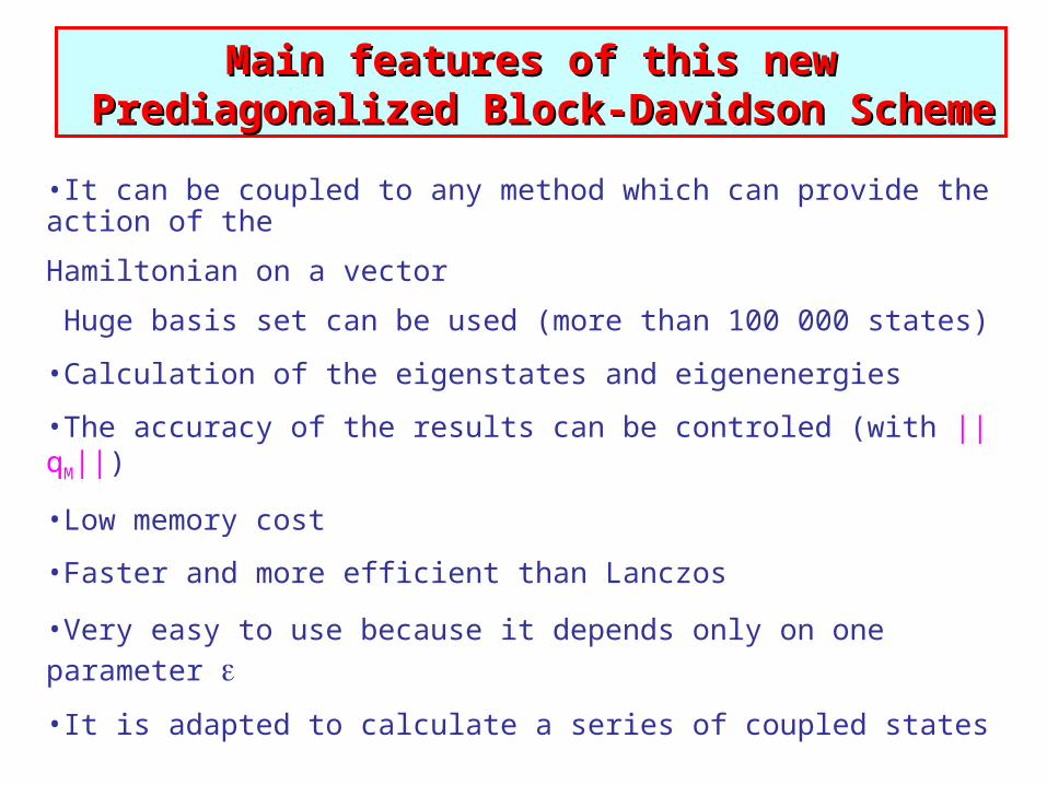
Main features of this newMain features of this new Prediagonalized Block-Davidson SchemePrediagonalized Block-Davidson Scheme

•It can be coupled to any method which can provide the action of the

Hamiltonian on a vector

Huge basis set can be used (more than 100 000 states)

•Calculation of the eigenstates and eigenenergies

•The accuracy of the results can be controled (with ||qM||)

•Low memory cost

•Faster and more efficient than Lanczos

•Very easy to use because it depends only on one parameter •It is adapted to calculate a series of coupled states

Conclusions

The development of a general method to calculate high excited ro-vibrational state is crucial Different approachs have to be exploited :

• The Jacobi-Wilson method coupled with the Davidson algorithm presents interesting

advantages.

•It allows the specific calculation of eigenstates associated with highly excited states

It can be improved by using a MC-SCF or SCF treatment

• However a lot of work has to be done… improve the fit of V, use a fit of the KEO in order to reduce

the CPU time…

3 – MCTDH Method (Time Dependant 3 – MCTDH Method (Time Dependant method) method)

A fit of the global PES has to be A fit of the global PES has to be performed : performed :

A factorized form of H is requiredA factorized form of H is required

Spectrum calculation •By Fourrier transform of the survival

probability•By filtered diagonalizationReferences :

H-D Meyer, U. Manthe and L. Cederbaum, Chem. Phys. Lett. 165, 73 (1990)M. Beck, A. Jaeckle, G. Worth and H-D Meyer, Physics Reports, 324,1 (2000)

C. Iung, F. Gatti and H-D Meyer, J. Chem. Phys., 120, 6992 (2004)

The MCTDH Approach

•Primitive Basis set : { |v1,…,v9>°,vi=0,1,…,vimax }

•The MCTDH « Active Space » is generated

by the configurations

: { i1(1)(Q1,t).. … i9

(2)(Q9 ,t); ij=0,1,…,ijmax ; j=1,…,9} :

(time-dependant functions which are adapted to the location of the wave-packet describing the system)

It is efficient if ijmax< vi

max

Time Dependent Coefficient and Functions to estimate

),()(...),,...,(3

1

)(

,,91

max

3

3

321

max

1

1

tjj

i

jt

jjjA

i

jt qQQ

Time dependent coefficient to optimize

LLL

JJ AHi I IA.

Projection on theSpace generated byFunctions j

() (Qk)

Time Dependent 3D functions to optimize

r

(1

(. (((

))1( H ( - Pi

Density Matrix Mean Field Hamiltonian

Application to the calculation of highly Application to the calculation of highly excited overtones in HFCO (|nexcited overtones in HFCO (|n66>)>)

Spectrum obtained with filtered DiagonalizationSpectrum obtained with filtered Diagonalization

10 0.31 + 0.51 10

Fraction of Energy in the different Normal Modes

The CH stretch is an

energy reservoir

106 206