DI

SC

US

SI

ON

P

AP

ER

S

ER

IE

S

Forschungsinstitut zur Zukunft der ArbeitInstitute for the Study of Labor

Pooling Multiple Case Studies Using Synthetic Controls: An Application to Minimum Wage Policies

IZA DP No. 8944

March 2015

Arindrajit DubeBen Zipperer

Pooling Multiple Case Studies Using Synthetic Controls: An Application to

Minimum Wage Policies

Arindrajit Dube University of Massachusetts Amherst

and IZA

Ben Zipperer Washington Center for Equitable Growth

Discussion Paper No. 8944 March 2015

IZA

P.O. Box 7240 53072 Bonn

Germany

Phone: +49-228-3894-0 Fax: +49-228-3894-180

E-mail: iza@iza.org

Any opinions expressed here are those of the author(s) and not those of IZA. Research published in this series may include views on policy, but the institute itself takes no institutional policy positions. The IZA research network is committed to the IZA Guiding Principles of Research Integrity. The Institute for the Study of Labor (IZA) in Bonn is a local and virtual international research center and a place of communication between science, politics and business. IZA is an independent nonprofit organization supported by Deutsche Post Foundation. The center is associated with the University of Bonn and offers a stimulating research environment through its international network, workshops and conferences, data service, project support, research visits and doctoral program. IZA engages in (i) original and internationally competitive research in all fields of labor economics, (ii) development of policy concepts, and (iii) dissemination of research results and concepts to the interested public. IZA Discussion Papers often represent preliminary work and are circulated to encourage discussion. Citation of such a paper should account for its provisional character. A revised version may be available directly from the author.

IZA Discussion Paper No. 8944 March 2015

ABSTRACT

Pooling Multiple Case Studies Using Synthetic Controls: An Application to Minimum Wage Policies*

We propose a simple, distribution-free method for pooling synthetic control case studies using the mean percentile rank. We also test for heterogeneous treatment effects using the distribution of estimated ranks, which has a known form. We propose a cross-validation based procedure for model selection. Using 29 cases of state minimum wage increases between 1979 and 2013, we find a sizable, positive and statistically significant effect on the average teen wage. We do detect heterogeneity in the wage elasticities, consistent with differential bites in the policy. In contrast, the employment estimates suggest a small constant effect not distinguishable from zero. JEL Classification: J38, J23, J88 Keywords: synthetic controls, program evaluation, heterogeneous treatment effects,

minimum wage Corresponding author: Arindrajit Dube Department of Economics Thompson Hall University of Massachusetts Amherst Amherst, MA 01003 USA E-mail: adube@econs.umass.edu

* We thank Joshua Angrist, Michael Ash, David Card, Michael Reich, Jesse Rothstein, Jeannette Wicks-Lim, and participants in the UC Berkeley IRLE seminar series and IZA-IFAU conference on labor market policies for helpful comments.

1 Introduction

The synthetic control o�ers a data driven method for choosing control groups that is valuable

for individual case studies (Abadie, Diamond and Hainmueller, 2010). This increasingly

popular technique generalizes the di�erence-in-di�erence estimator o�ering a factor-based

approach to control for time-varying confounders. For a single state that receives a policy

treatment, the synthetic control is the weighted average of untreated units that best predicts

the treated state in the pre-treatment period, and the estimator is the post-treatment di�erence

between the treated state and its synthetic control. Whereas conventional regression designs

equally weight all units (conditional on covariates), units comprising the synthetic control

typically receive unequal weights. Matching on pre-treatment outcomes allows the synthetic

control approach to provide unbiased estimates for case studies even when there are multiple

unobserved time factors, unlike the conventional di�erence-in-di�erence model which imposes

a single factor assumption.

A growing number of papers have used the synthetic control approach to study topics

as diverse as the impacts of anti-smoking legislation (Abadie et al., 2010), immigration

laws (Bohn et al. 2014), and minimum wages (Sabia et al. 2012). However, to date the

applications have largely been restricted to estimating the e�ect of individual treated cases

or to presenting numerous such estimates separately. For example, Billmeier and Nannicini

(2013) use synthetic controls to investigate the e�ects of 30 country-level episodes of trade

liberalization on their GDP. While the authors helpfully organize their presentation of

synthetic and actual GDP trends by region and time period, the presentation of 30 individual

pictures obscures their argument that later episodes of liberalization failed to boost GDP.

Some episodes appear to raise, lower, or have no e�ect on growth, and it becomes di�cult

for the reader to gauge the magnitude of estimates or to draw statistical inference. Using

synthetic controls, Campos et al. (2014) estimate a mean e�ect of EU integration on GDP,

but the authors do not perform statistical inference on either the mean or individual case

study estimates.

2

In this paper, we present a method for pooling synthetic control estimates in a setting

with recurring treatment and variable treatment intensity: state-level minimum wage changes.

Because the intensity of the treatment varies across cases, we convert the estimates to

elasticities by scaling them by the size of the minimum wage changes, and then aggregate

these elasticities across events. A key contribution of the paper shows how the mean of the

percentile ranks of the e�ects in the treated states vis-à-vis donor (or potential control) states

can be used to judge the statistical significance for the pooled Hodges Jr. and Lehmann (1963)

point estimate. Pooling the estimates using their ranks is particularly useful since the exact

distribution of the sum (or mean) of the ranks under the null is known, enabling us to perform

exact inference that is valid for small samples. Additionally, we invert the mean rank statistic

to construct the confidence interval for the pooled estimate. Our approach of pooling across

treated units is closely related to the van Elteren (1960) stratified rank sum test. It is also a

natural extension of the placebo-based inference used by Abadie et al. (2010) for a single case

study, where the distribution of a test statistic under the null is constructed by randomly

permuting the treatment status of the donor units. Our inferential procedure has some

similarity to Conley and Taber (2011); operating under the classic di�erence-in-di�erence

context, they also use information from control units to form an empirical distribution under

the null, and invert the test statistic to construct confidence intervals that are valid with a

small number of treated cases. Finally, Dube et al. (2011) also use a average rank-based test

that is valid for small samples in the context of financial market event studies.

Since percentile ranks of the estimates have a known distribution under the null hypothesis,

exact inference is feasible not only for the mean but also distributional statistics as well.

In this paper we use the Kolmogorov-Smirnov and Anderson-Darling tests to determine

whether the distribution of ranked e�ects indicates heterogeneous treatment e�ects. One

concern when pooling across events is that the quality of the match between the treated and

synthetic control unit may be poor in some instances. We assess the role of match quality by

trimming on pre-intervention goodness of fit as determined by the mean squared prediction

3

error (MSPE). A final contribution of the paper concerns the choice of predictor variables,

since there is little guidance on this issue in the existing literature. We use a cross-validation

criterion of minimizing MSPE among donor units to choose between alternative sets of

predictors.

The minimum wage o�ers an interesting setting for applying the synthetic control estimator,

since states receiving treatment have important di�erences that appear to vary over time,

thereby confounding the canonical two-way fixed e�ects panel estimator (Allegretto et al.,

2013). Since the synthetic control method depends on isolated treatment events with well-

defined pre- and post-treatment periods, the approach can only utilize a limited amount of

minimum wage variation available to conventional regression techniques. We select those

events with no minimum wage changes two years prior to treatment and with at least one

year of post-treatment data, which we consider to be the minimal requirement for measuring

the policy’s impact. Of the 215 state minimum wage changes during our 1979-2013 study

period, only 29 meet our minimal criteria; on average these events have a 19 quarters of data

prior to the intervention and 10 quarters afterward. While this is a limited number of events,

we show that pooling across these 29 cases provides us with su�cient statistical power to

detect economically relevant e�ects posited in the literature.

Our results show that the minimum wage changes were binding: 25 out of the 19 cases

have positive e�ects on average teen wage, with a median elasticity of 0.24 and mean of 0.37.

The pooled Hodges-Lehman elasticity of 0.266 is statistically significant at the one percent

level using our mean rank test. Turning to teen employment, we find 12 positive elasticities

and 17 negative ones. Both the median (-0.051) and mean (-0.058) estimates are small in

magnitude. The mean percentile rank is 0.497 and the associated pooled Hodges-Lehman

elasticity is -0.036. With a 95 percent confidence interval, we rule out a pooled employment

elasticity more negative than -0.170. The distribution of the ranked wage estimates indicate

a heterogeneity in the impact, consistent with some minimum wage increases having more

“bite,” a�ecting a larger share of the teen workforce. In contrast, the distribution of the

4

ranked employment estimates is consistent with the sharp null of a small (possibly zero)

e�ect everywhere, as opposed to an averaging of true positive and true negative e�ects across

events. To address concerns about match quality, we show that our results are similar when

we limit our case studies to those with better pre-treatment fit. We do note that the treated

states are generally some of the highest wage areas, making it di�cult to find a convex

combination of donors to very closely match the average wage level in the pre-intervention

period. However, this does not a�ect our ability to match their overall employment dynamics

prior to the intervention.

Three papers in the minimum wage literature have particular relevance to the application

of synthetic controls. An early precursor to synthetic controls is the study of California’s 1988

minimum wage change by Card (1992). Card compares California with an aggregated control

comprised of four southern states and one metro area that failed to raise their minimum

wages during the 1987-1989 period. Similar to the synthetic control approach, the aggregated

control in Card (1992) roughly matches California on several pre-treatment labor market and

demographic characteristics. However, Card’s selection of the donor states is heuristic and

not based on a solution to the explicit optimization problem underlying the contemporary

synthetic control approach.1

More recently, Sabia et al. (2012) uses the synthetic control approach to study the impact

of the 2005 New York minimum wage increase. They ignore four other candidate treatment

events that also began the same year in Florida, Minnesota, New Jersey, and Wisconsin.

It is not clear what guided the authors’ selection of New York as the sole case; in our

results for these five states, we find that the New York event is associated with a fairly

negative employment estimate. Sabia et al. (2012) also crucially fail to use any pre-treatment

outcomes as predictors. Although any characteristics una�ected by the policy treatment are

1The 1988 minimum wage increase in California is one of our 29 events. We find a positive wage andemployment point estimates for teens, which is broadly consistent with Card’s findings. However, both theemployment and wage elasticities are highly imprecise, with wide confidence intervals containing positive andnegative values. This highlights the di�culty in learning very much from an individual case study—a pointalso stressed by Dube et al. (2010) in the context of pooling across case studies using contiguous area controls.

5

valid predictors under the synthetic control approach, some combination of pre-intervention

outcomes should be included. Intuitively, if the synthetic control fits a su�ciently large set

of pre-intervention outcomes, it is able to account for any number of time-varying factors.2

As a result of omitting pre-intervention outcomes, the authors obtain a likely unreliable

counterfactual: specifically, employment paths for actual and synthetic New York never

coincide during the entire 2000-2004 pre-treatment period.3

Neumark et al. (2014) use a panel estimator loosely based on the synthetic control method.

Allegretto et al. (2013) discusses in detail the problems with this approach. First, they do not

actually pool individual synthetic control estimates. Instead, they stack the treated units and

the synthetic controls and estimate a two-way fixed e�ect model using the stacked data with

log minimum wage as the main independent variable. Unlike a standard synthetic control

study, their estimator does not limit identifying variation to be within a matched pair of

treated state and its synthetic control. Rather, it also uses variation in the minimum wage

between all treated and synthetic control units, which is di�cult to justify within a synthetic

control approach. Second, in their setup both treatment and potential control units are

experiencing minimum wage changes, making the distinction between treatment and control

units somewhat meaningless. Moreover, they experience minimum wage changes both before

and after “treatment,” making the before/after distinction somewhat meaningless as well.

Since the synthetic control approach requires a clean pre-intervention period and untreated

donors to correctly estimate the donor weights, the violation of these assumptions makes

the donor weights they estimate unreliable. Finally, they use a very short pre-intervention

window (4 quarters) to calculate synthetic control matches, which makes finding a good

match di�cult.

2Formally, the unbiasedness of the synthetic control estimator relies specifically on pre-treatment outcomebalance between the treated unit and the weighted combination of donors (see Appendix B of Abadie et al.(2010)). The choice of exactly which pre-treatment outcomes and other characteristics to select as predictorvariables is not obvious, a priori. We provide guidance for these decisions in section 3.2.

3See Figure 3 of Sabia et al. (2012). Relatedly, the authors try to account for the poor pre-interventionfit by using a di�erence-in-di�erence with respect to the synthetic control. While this has a heuristic appeal,it is quite di�erent from the synthetic control estimator, which requires the pre-intervention values in thetreated and synthetic control units to be close.

6

In contrast to these prior applications, we select 29 di�erent events using clear (and

reasonable) criteria for case selection, estimate synthetic controls for each treatment using a

data-driven choice of predictors, and pool across these estimates using rigorous statistical

procedures that are valid for small samples.

This paper also relates to a growing literature that use linear factor models to account for

time-varying heterogeneity in program evaluation, e.g., Bai (2009). Gobillon and Magnac

(2015) provide evidence comparing the performance of alternative estimators using Monte

Carlo simulation.4 In work carried out contemporaneously with our own, a recent working

paper by Totty (2014) applies linear factor models such as Bai (2009) to estimate minimum

wage e�ects and finds results that are broadly similar to those we estimate here using a

pooled synthetic control approach.

The rest of the paper is structured as follows. Section 2 reviews the synthetic control

method and explains our proposed rank-based inference for the pooled estimate. Section

3 discuss our sample and the choice of predictor variables. Section 4 presents our findings,

including the mean e�ect and the test of heterogeneity, as well as issues of match quality.

Section 5 concludes.

2 Synthetic controls and multiple case studies

2.1 Synthetic control estimator

Consider the case of a single treated state (i = 1) that raises its minimum wage at time t = tÕ,

where the outcome of interest Yit

is teen employment. Denoting the intervention as D, the

synthetic control approach assumes a data generating process such that the observed outcome

4We became aware of the Gobillon and Magnac (2015) paper, which also discusses a method for poolingsynthetic control studies, after we began working on this paper. Their proposed method is similar to one ofthe four methods of inference we evaluate—namely randomization inference using the mean e�ect in section4.5. We note that our rank-based aggregation has a number of advantages, because it allows exact inferenceusing a known distribution. Moreover, we use the distribution of ranked e�ects to assess heterogeneity of thetreatment e�ects.

7

Yit

is a sum of the e�ect from the treatment, –1t

Dit

, and the counterfactual outcome, Y N

it

:

Yit

= –it

Dit

+ Y N

it

= –it

Dit

+ ◊t

Zi

+ ⁄t

µi

+ ”t

+ ‘it

.

Here ”t

is an unknown common factor with constant factor loadings across units, Zi

is a

(1 ◊ r) vector of observed covariates una�ected by the intervention, and ◊t

is a vector of

unknown parameters. Like the standard fixed e�ects model, there is a common time factor

”t

. However, there is an additional ⁄t

µi

term as well. Here ⁄t

is a vector of unobserved

time-varying factors and µi

are the unknown factor loadings. Since the factor loadings can

vary across states, treatment and control states need not follow parallel trends, conditional on

observables. If we knew the true factor loadings µ1 for the treated state, we could construct

an unbiased control by taking untreated donor states whose factor loadings average to µ1.

Since we do not observe the factor loadings, the synthetic control procedure constructs a

vector of weights W over J donor states such that the weighted combination of donor states

closely matches the treated state in pre-intervention outcomes. This weighted combination of

donors is called the synthetic control; as shown in Abadie et al. (2010), the average factor

loadings of the synthetic control thus constructed matches the loadings of the treated state.

Formally, for the treated state, define the (k ◊ 1) vector of pre-treatment characteristics

as X1 =1ZÕ

1, Y K1i

, . . . , Y KLi

2, where k = r + L and Y Kl

i

are L linear combinations of

pre-treatment outcomes. Analogously, define the k ◊ J matrix X0 containing the same

characteristics for the J donor states. The synthetic control procedure chooses donor weights

W to minimize the distance between pre-treatment characteristics X1 and X0 of the treated

state and untreated states. The distance equals the mean square prediction error (MSPE)

kÿ

m=1v

m

(X1m

≠ X0m

W)2

over k pre-treatment characteristics, and where vm

measures relative importance of the m-th

predictor. Given the optimal weights wúj

for each of the j = 2, . . . , N donors, the synthetic

8

control at any time t is simply the weighted combination of donor employment qN

j=2 wúj

Yjt

.

The estimate of the employment impact –1t

is therefore the di�erence between employment

in the treated state Y1t

and the synthetic state qj

wúj

Yjt

at any post-treatment time t > tÕ:

–1t

= Y1t

≠Nÿ

j=2wú

j

Yjt

.

When the intensity of treatment varies across events, elasticities o�er a simple way of

comparing across events. Moreover, the use of elasticities also connects our findings with

other estimates in the minimum wage literature. For this reason, our key estimates of interest

are the employment or wage elasticities of the minimum wage, defined as follows. For a single

treatment event, we construct the synthetic control qj

wúj

Yjt

for the treated outcome Y1t

. In

the post-intervention period t = tÕ, . . . , T , the average percent di�erence between the treated

and synthetic control outcomes is given by

—1 =1T

qT

t=t

Õ

1Y1t

≠ qj

wúj

Yjt

2

1T

qT

t=t

Õq

j

wúj

Yjt

.

Writing the percent minimum wage increase over the full post-treatment period as

�MW = MWT

≠ MWt

Õ≠1MW

t

Õ≠1

we define the post-treatment elasticity ÷1 to be the ratio

÷1 = —1�MW

.

As we describe below, it will be useful for placebo-based inference to construct analogous

elasticities ÷j

for each of the donor states. Specifically, for each of the donor states j = 2, . . . , N

we calculate the post-treatment di�erence —j

, this time using the remaining N ≠ 2 donor

states as donors for the synthetic control of state j. The placebo elasticity ÷j

is scaled by the

9

actual minimum wage increase in treated state: ÷j

= —j

/�MW .5

When there are multiple treatment events, we calculate separate event-specific elasticities

÷e1 = —

ej

/�MWe

for the events e = 1, . . . , E. Note that this construction of elasticities

allows us to incorporate the fact that treated states vary both in their outcome levels and in

their minimum wage treatment intensities. To aggregate across events we calculate the mean

or median of these estimated elasticities, or calculate the Hodges-Lehman pooled estimate

as described in detail below. The mean treatment e�ect, for example, is equal to the mean

elasticity

÷ =q

e

÷e1

E.

2.2 Inference using the rank test with single and multiple events

We follow Abadie et al. (2010) in using placebo-based inference from permuting the treatment

status of donor states in order to assess the statistical significance of a single treated state’s

estimated elasticity. For each event, we estimate ÷ej

for every donor state j (excluding the

actually treated state but using the same minimum wage change) and determine whether the

elasticity ÷e1 for the treated state lies in the tails of the resulting placebo distribution formed

by ÷ej

for j = 2, . . . , Ne

. Like Abadie et al. (2010), we assume exchangeability of units for

the purpose of conducting statistical inference throughout the paper.

Equivalently, we summarize the relative position of the treated state’s elasticity among

the placebo distribution by using the percentile rank statistic pe1 = F

e

(÷e1), where F

e

is the

empirical CDF of the elasticities ÷ej

from event e.6 Since the percentile rank is (approximately)

uniformly distributed on the unit interval, we determine whether the rank of the treated5As we discuss in Section 3, since some states change their minimum wage multiple times during the

post-treatment period, we simply define the minimum wage change to be the largest percent change betweenthe post- and pre-treatment periods. We define the elasticity ÷1 using the ratio of means in —1 rather thanthe post-treatment mean of the percent changes 1

T

qTt=tÕ

3Y1t≠

qj

wúj Yjtq

jwú

j Yjt

4to avoid the possibility that the

resulting elasticity has a di�erent sign than the post-treatment mean of level changes in the numerator of —1.6To calculate the percentile pei of the ranked position rei of the estimated elasticity ÷ej for state i in

event e, we use the Weibull-Gumbel rule (see Hyndman and Fan, 1996): pe = re1/(Ne + 1), where Ne equalsone plus the number of donor states, ensuring that the median e�ect within an event receives the rank 0.50when the total number of states Ne is odd.

10

state pe1 lies in the tails of the uniform distribution. Using a statistical significance level of

five percent, we reject the null of ÷e1 = 0 precisely when p

e1 < 0.025 or pe1 > 0.975. We note

that the number of available donors limits the range of confidence levels we can implement

for a single treated event. For example, many of our events have only twenty donors; in these

cases we can only assess a ten percent level of significance. Using multiple events allows us to

assess stronger levels of statistical confidence.

The above approach suggests a natural way of conducting inference when pooling across

cases by constructing a test statistic p which is the the mean of the percentile ranks of

individual events:

p =q

E

e=1 pe

E.

The exact distribution of p can be calculated using the Irwin-Hall distribution of the sum of

E independent uniform random variables. The sum of the ranks, s = E · p, has the the CDF

�(s; E) = 1E!

ÂsÊÿ

k=0(≠1)k

AE

k

B

(s ≠ k)E≠1

where Â.Ê is the floor function.7 Under the sharp null hypothesis of zero e�ect everywhere,

the average of E ranks, p, is distributed with mean 0.5. If G(x; E) = �(x · E; E) denotes

the CDF of the mean of E uniformly distributed variables random variables, then for a

statistical significance level of five percent, we reject the null hypothesis ÷ = 0 precisely when

G(p; E) < 0.025 or G(p; E) > 0.975.

While the central limit theorem tells us that the distribution of the mean rank will converge

to an appropriately scaled normal distribution, for small E we should prefer to use the exact

distribution. Table A1 shows various percentiles of this distribution for E = 1, . . . , 30. At

29 treatment events—the maximum number of case studies we will have in our study—a

two-sided 5% significance test requires the mean rank to fall below 0.395 or above 0.605. We

7See http://en.wikipedia.org/wiki/Irwin-Hall_distribution.

11

note that this method is closely related to the van Elteren (1960) stratified rank sum test,

where the rank of each treatment is estimated using placebos associated with the stratum (i.e.,

event). The only substantive di�erence is that we use the percentile ranks of each treatment

from each stratum, pe1, instead of the ranked position r

e1, for transparency of the calculations;

this choice potentially impacts the critical values when the number of observations (states)

varies across strata (events) and the number of observations is also small. However, as we

show in section 4.5, there is very little di�erence if we calculate the critical values taking

into account the number of observations in each stratum used to calculate the ranks. For

concision, in the rest of this paper we will often we refer to the percentile rank as simply the

“rank.”

While there are alternative ways of doing pooled inference, we note some advantages to

our approach. First, the rank-based pooling is a natural generalization of the single-case

study based inference in Abadie et al. (2010), who use the rank of the treatment e�ect for

individual events. Second, the mean (or sum of) ranks has a known distribution under the

sharp null, allowing for exact inference. This avoids reliance on large sample properties,

and also avoids the empirical estimation of distribution of the statistic under the null—as

would be the case were we, for example, to conduct inference for the mean elasticity. Third,

and relatedly, the use of the mean rank p diminishes the impact of outliers as compared to

the mean elasticity ÷, which may be a particular concern given a small number of events.

Fourth, within the class of rank sum tests, the ranks could be estimated without regard to

strata, as in the case of the Wilcoxon (1945) rank sum test. However, stratification accounts

for event-wise heteroscedasticity, which may be of particular concern given varying window

lengths across events. One limitation of the rank-based pooling is that we are testing the

sharp null that e�ect is zero everywhere, as opposed to the average e�ect being zero. However,

we address this concern in Section 4.3 by testing for heterogeneous treatment e�ects.

In section 4.5, we relax the approximation that the event ranks are independently and

uniformly distribution by accounting for the finite number of donors, some of which overlap

12

across events. We show that in our case this makes little di�erence to the calculation of the

critical values, or the resulting confidence intervals for the treatment e�ect. For comparison,

we also calculate the confidence interval using randomization inference on the mean e�ect

(elasticity), as opposed to using the mean rank. This too produces similar conclusions, though

the confidence intervals are somewhat wider—consistent with the impact of outliers when

evaluating the mean (as opposed to the ranked) e�ect.

2.3 Inverting the rank test to form confidence intervals

We also invert the individual-event and mean rank statistic to estimate confidence sets.8 These

confidence sets show values of the elasticities which imposed as the null cannot be rejected as

being equal to the estimated e�ect. For a single treatment event with estimated elasticity

÷e1, we use the percentile rank p

e1 = Fe

(÷e1) as the test statistic to determine statistical

significance: we cannot reject the null hypothesis ÷e1 = 0 at the five percent level precisely

when 0.025 Æ Fe

(÷e1) Æ 0.975. Inverting this test, we ask for what values of · does the

adjusted response ÷e1 ≠· appear free from treatment: when does 0.025 Æ F

e

(÷e1 ≠·) Æ 0.975?

The 95 percent confidence interval is the set of · not rejected using the critical values 0.025

and 0.0975.

In the framework of multiple treatment events, we can apply a similar procedure to

construct Hodges Jr. and Lehmann (1963) confidence intervals for the pooled e�ect, using

the mean rank p as the test statistic to be inverted. We first calculate the adjusted responses

÷e1 ≠ · for all events e = 1, ..., E, and re-calculate event-specific ranks F

e

(÷e1 ≠ ·). Define

the mean adjusted rank

p(·) =q

e

Fe

(÷e1 ≠ ·)

E.

The 95 percent confidence interval for the pooled e�ect is the set of · such the mean adjusted

rank p(·) lies within the critical values given by the mean of E uniform distributions. In

8Although Abadie et al. (2010) do not explicitly construct these confidence sets in the case of their singletreatment event, they follow directly from their inferential procedure.

13

other words, we find values · such that 0.025 < G(p(·); E) < 0.975. Figure 1 illustrates this

procedure for the estimated mean elasticity ÷ = c. The confidence interval is (c ≠ b, c + a)

because G(p(c ≠ (c + a)); E) = 0.05 and G(p(c ≠ (c ≠ b)); E) = 0.95.

Collapsing these confidence intervals yields the Hodges-Lehman point estimate, which

we also refer to as the pooled estimate in this paper. In the case of a single event, the

mean, median, and Hodges-Lehman point estimates are trivially the same, and so are the

confidence intervals. In the case of multiple events, the mean, median and Hodges-Lehman

point estimate and confidence intervals need not correspond. This is especially the case

when outlying estimates of individual treatment events heavily influence the mean estimate.

The robustness to outliers is one reason we prefer using the Hodges-Lehman confidence

interval, as it is ultimately based on ranked location. Throughout the paper, we report the

mean percentile rank, the pooled Hodges-Lehman point estimate, and the Hodges-Lehmann

confidence intervals. We also report the median and mean estimates because of their natural

interpretations.

Our inference assumes that the ranks of the treated states across events are independent

draws. There are two potential concerns with this assumption, but overall we do not believe

they represent major problems in our case. First, some events are from the same state, which

may bring up a concern that the ranks of the events are not independent draws. However,

while Yit

may be serially correlated, the same need not be true for ÷eit

across two events eÕ and

eÕÕ from the same state i in time periods tÕ and tÕÕ. If the synthetic control estimator is unbiased,

and it successfully matches pre-treatment outcomes of both events, the post-treatment gap

would from the two events are (by construction) uncorrelated: E(÷e

Õ1, ÷e

ÕÕ1) = 0. Moreover,

this can be verified empirically.

The second and more serious concern is that the because the minimum wage increases

often occur around the same time, two states with minimum wage increases may share many

of the same potential donors. As a result, the ranks determined by the placebo distributions

are not truly independent across treatment events. For two events eÕ and eÕÕ, the set of placebo

14

estimates ÷e

Õqt

Õ and ÷e

Õqt

ÕÕ from donor q may be correlated, in particular when tÕ = tÕÕ. In the

extreme case, the donors and hence the placebo estimates –e

Õqt

Õ may be identical. This may

induce a correlation in the ranks Fe

Õ(÷e

Õ1) and Fe

ÕÕ(÷e

ÕÕ1) even though E(÷e

Õ1, ÷e

ÕÕ1) = 0 . In

reality the overlap in donor pool is only partial, which mitigates this problem. However, since

this may be a concern in other applications, we provide a more computationally intensive (but

more accurate) method of constructing the critical values for hypothesis testing in section

4.5. As described further in that section, we draw sets of 29 placebo-law interventions that

match the timing and donor overlap patterns of the actual 29 treatments in our sample. The

results suggest that accounting for donor overlap has little impact on the estimated critical

values, justifying our use of the mean of independent uniform distributions.

3 Minimum wage treatment events and empirical spec-

ification

3.1 Sample periods and timing of treatment

The synthetic control estimator requires a set of untreated or donor units for each treatment

event. Since the vast majority of states were a�ected by the federal minimum wage increases,

federal increases are not suitable for use with the synthetic control method: there are very

few untreated donors that can be drawn from to construct a synthetic control for a�ected

states. For example, 45 states changed their minimum wage at some point during the year of

the 2007 federal minimum wage increase, leaving only 5 states as potential donors to form

synthetic controls.

To maximize the number of treatment events, we consider the entire 1979-2013 period

available using Current Population Survey (CPS) data. We focus on teen employment and

wages, as many 16- to 19-year olds have wages near the minimum. During this period, almost

38 percent of teens received wages within 10% of the statutory minimum wage, compared

15

with about 5% of workers aged 20 to 64. While there is considerable debate regarding the size

of teen employment e�ects, we expect to find significantly positive e�ects on teen wages. The

high incidence of minimum wage workers among teens makes them the most frequently studied

group in the minimum wage literature (e.g., Neumark et al. 2014, Allegretto et al. 2013). For

outcome variables we calculate quarterly state-level teen employment-to-population ratios and

average wages using the CPS.9 Although annual state means would contain less noise, they

would correspondingly limit the number of pre- and post-treatment observations; moreover,

not all minimum wage increases occur during the same part of the calendar year.

The top panel of Figure 2 shows all quarterly minimum wage changes during the study

period.10 During this period the federal minimum wage increased nine times, indicated by

the vertical lines in the Figure. Aside from federal minimum wage changes, 33 states in this

period raised their minimum wage 215 times. Many states increase their minimum wage

frequently, often on an annual basis. To utilize the synthetic control method, we limit the

sample of usable treatment events to those with well-defined pre- and post-treatment periods.

We select those events with no minimum wage changes two-to-eight years prior to treatment,

and we require at least one year of post-treatment data (eliminating from consideration very

recent minimum wage changes in Rhode Island and Missouri).We also limit the sample to

minimum wage increases of at least 5 percent, which discards states with small increases

indexed to inflation. Finally, we only consider treatment events with at least 5 untreated

states so that there are a su�cient number of potential donor states to form synthetic controls.

These restrictions reduce the pool of state-level minimum wage increases by more than 88

percent and yield the 29 treatment events in the top panel of Figure 2 labeled in dark text.

The eligible 29 events have valid pre- and post-treatment periods of varying length. West

9For employment outcomes we use the Unicon CPS extracts for the monthly Basic Survey (http://unicon.com). Wage data is only available in the outgoing rotation group subset of these data; for wagedata, we use the NBER Merged Outgoing Rotation Group extracts (http://www.nber.org/morg/annual/).We calculate wages as hourly earnings or, if these are not reported, weekly earnings divided by usual weeklyhours. State-quarter-level averages use the sampling weights.

10We thank Sylvia Allegretto for providing monthly historical minimum data, which we convert to quarterlyaverages.

16

Virginia, for example, has many years of data prior to its minimum wage change in 2006q3

available but only one year of post-treatment data. By contrast, California’s treatment in

2001q1 allows only two years of clean pre-treatment data but many years of post-treatment

data. Also, California’s post-treatment period includes an additional minimum wage increase

in 2002q1. To simplify choices, for each event we select its “maximal” pre-treatment period

available from 8-32 quarters; having done so, we then select each event’s maximal post-

treatment window from 4-12 quarters. The bottom panel of Figure 2 illustrates these pre-

and post-treatment selections in blue and red, respectively, with red circles indicating the

times of treatment. Two features stand out. First, while the pre-treatment period contains no

minimum wage increases by definition, the post-treatment period includes multiple minimum

wage changes—states that raise their minimum wage often do so again within the next year

or two. Table 1, which lists all 29 treatment event configurations that form the basis for our

primary specifications, shows that most events include multiple minimum wage increases.

There are four events whose post-treatment period includes four minimum wage increases.

For this reason our treatment intensity definition incorporates the maximum minimum wage

in the post-treatment period.

Second, Figure 2 there are three states in the 2000s with recurring minimum wage changes

where the post-treatment period of one minimum wage change overlaps with the pre-treatment

period of a later minimum wage change: Hawaii, Rhode Island, and Vermont. For example,

Hawaii’s post-treatment period for its 2002q1 treatment overlaps with the pre-treatment

period of Hawaii’s 2006q1 treatment. Delayed e�ects from the former 2002q1 treatment could

in principle violate the assumption that, for the latter 2006q1 event, Hawaii’s pre-treatment

period is absent from treatment. On the other hand, the pre-treatment period of Hawaii’s

2006q1 is absent from treatment using our original definition that it contains no minimum

wage changes. For our primary specifications we will include all 29 events, but we will also

describe results excluding the three events of Hawaii 2006q1, Rhode Island 2006q1, and

Vermont 2004q1.

17

There is a trade-o� between window length and the number of events and donors. Allowing

relatively short pre- and post-treatment periods maximizes the number of treatment events

but, at the same time, may reduce the quality of the estimated counterfactual, as there is less

pre-treatment data informing the selection of synthetic controls. On the other hand, lengthy

pre-treatment periods limit both the number of events and potential donors, thereby reducing

the credibility the resulting estimates. When we limit our treatment events to those with

more restrictive pre- and post-treatment window lengths, we sharply reduce the number of

case studies, as Table 2 illustrates. The first line in Table 2 is our primary configuration: 29

events with at least 8 and 4 quarters of respective pre- and post-treatment data. Requiring

pre-treatment and post-treatment windows of at least 16 and 8 quarters, respectively, curtails

the number of case studies to 14, and there is only a single treatment event with the most

restrictive window configuration of 32 pre-treatment quarters. In terms of the potential for

alternative window configurations to a�ect donor availability, the configurations in Table

2 show only a small amount of variation. As we limit the pool of case studies to the most

restrictive window configurations, the mean minimum wage treatment rises a small amount,

from about a 19 percent increase to an increase of about 24 percent when we require 6

years and 2 years of pre- and post-treatment data, respectively. Our primary results use the

maximal window configuration with 29 events, but we explore how the alternate window

configurations a�ect our results in Section 4.3.

3.2 Specifying predictor variables

Any characteristics una�ected by the policy intervention are valid predictors under the

synthetic control approach, including demographic and industrial compositions or other

economic attributes of the region. However, the unbiasedness of the estimator relies on the

predictors including some linear combination of the pre-treatment values of the outcome of

interest. There are two related questions when it comes to these predictors. First, exactly

which variables should one include in the set of predictors? Second, what weight should one

18

place on each of those predictor variables when estimating the donor weights? Abadie et

al. (2010) provides a simple answer to the second question of how best to determine the

weights on specific predictors within a set, which we describe first. Then we tackle the more

challenging question of what predictors—and specifically what pre-treatment outcomes—one

should include in this set.

For a given event e, the optimal donor weights are defined as

Wúe

(Ve

) = argminWe

kÿ

m

vm

(Xe1m

≠ Xe0m

We

)2 . (1)

The optimal weights depend on the predictor importance matrix Ve

= {vem

} selected by

the researcher. For example, V might weight each predictor equally. Instead we follow the

suggestion in Abadie et al. (2010) to select Vúe

such that the resulting synthetic control best

fits pre-treatment outcomes. We therefore solve the joint (nested) optimization problem given

by equation 1 and the equation

Vúe

= argminVe

ÿ

t<t

Õe

(Ye1t

≠ Ye0t

W(Ve

))2

which minimizes pre-treatment fit. Our results use the “optimal” choice of weights Wúe

(Vúe

)

instead of alternatives such as manually specifying weights for predictors, or using the

computationally less intensive methods available to users.11

But exactly which sets of pre-treatment outcomes and other characteristics should the

researcher choose as predictors? When computationally feasible, perhaps the simplest strategy

is to include every pre-treatment outcome in the predictor set X. In their study of the e�ects

of Arizona’s 2007 Legal Arizona Workers Act, Bohn et al. (2014) employ this strategy with

annual CPS data, using every pre-treatment value of the 1998-2006 non-citizen Hispanic

11We implement the synthetic control approach in Stata using the synth package with nested optimizationand allopt starting point checks for robustness: http://www.mit.edu/~jhainm/synthpage.html. There isa option for using a less computationally intensive but less reliable “regression-based” predictor weights.In our experience, the regression-based weights can produce worse fit, and the nested optimization usesregression-based weights as an initial set of values for optimization.

19

share of the population, in addition to other industrial and demographic shares.

Within the pre-intervention sample, one cannot do any better in terms of pre-intervention

MSPE than to include every pre-intervention outcome. However, this will not be true when

predicting out of the pre-intervention sample, which is ultimately the object of interest.

Matching on higher frequency pre-intervention data may actually produce less reliable

synthetic controls. For example, our study uses quarterly CPS data, we risk matching on

noise when using as predictors every quarterly pre-treatment value of teen employment-

to-population ratios or average wages. As a result, we also consider the predictor set X

consisting of annualized averages of the pre-treatment outcome.12

Di�erent sets of predictors may result in di�erent synthetic controls, and there is little

explicit guidance in the synthetic control literature to assess predictor choice. We consider

four di�erent predictor sets X, which vary according to whether we include every quarterly

or annualized pre-treatment outcome, and whether we include other pre-treatment average

demographic, labor market, industry shares.13 These predictor sets are summarized at the

bottom of Table 3. Using teen employment as an example outcome, predictor set 1 is composed

of all quarterly pre-treatment values of teen employment-to-population ratios. Predictor set

2 is composed of all annualized pre-treatment employment-to-population ratios. Predictor

set 3 includes all annualized pre-treatment employment and wage outcomes. Predictor set 4

adds to predictor set 3 the pre-treatment demographic, labor market, and industry shares

described above. We note that when every quarterly pre-intervention outcome is included in

the predictor set, inclusion of other predictor variables is redundant when weights on those

predictors are calculated optimally using nested optimization. For this reason, it only makes

12Here, annualized averages refer to the mean of the first through fourth quarter before treatment, themean of the fifth through the eighth quarter before treatment, etc. For Minnesota’s 2005q3 treatment, say,these refer to the 2004q3-2005q2 mean, the 2003q3-2004q2 mean, etc.

13The demographic and labor market variables are the pre-treatment means of white, black, female,and married shares of the teen population, the teen population share, the share of the overall populationwith a college degree, and the overall unemployment rate. Industry variables are the employment sharesin agriculture & mining, construction, manufacturing, wholesale & retail trade, transportation & utilities,information/finance/professional/business services, education & health services, leisure/hospitality/personalservices, and public administration.

20

sense to include variables such as industry or demographic shares when using annualized and

not quarterly pre-treatment outcomes.

To identify the “best” choice for X, we use a cross-validation procedure to choose from

di�erent sets of predictors. Recall that in creating synthetic controls for each event, the

pre-intervention observations form a “training sample” used to estimate synthetic control

donor weights as well as predictor weights for a given set of predictors. Here, when choosing

the most reliable set of predictors, we use the post-intervention observations of the donors as

our “validation” sample to evaluate prediction error associated with a given set of predictors.

For a given predictor set X, we calculate the post-treatment mean-squared prediction error

(MSPE) for each donor j given by

MSPEej

= 1T

e

Teÿ

t=t

Õe

A

Yjte

≠ÿ

q

wúeq

Yeqt

B2

where tÕe

begins the post-treatment period in event e, and where q indexes the available N ≠ 2

donors for (untreated) state j. We define the average RMSPE to be the square root of the

mean of this quantity across all donors for all 29 events. The optimal model will yield the

smallest post-treatment RMSPE, so predictor sets X with higher average RMSPE in the

post-treatment period indicate models with worse performance in the sample of untreated

donors.14

Table 3 reports the average donor RMSPE for both the post-treatment (validation) and

pre-treatment (training) samples across four candidate specifications for predictors. Predictor

set 1, which uses quarterly pre-treatment outcomes, naturally obtains the best pre-treatment

fit to quarterly employment or wages when compared to predictor sets 2 through 4, which try

to fit quarterly frequency data using annualized pre-treatment outcomes. Incorporating both

annualized outcomes and additional controls improves pre-treatment fit relative to using only

one annualized outcome: for employment, pre-treatment RMSPE falls from about 0.040 in

14We do not use the treated states for this cross-validation exercise because use of the post-treatmentperiod in these states would require us to also have a valid estimate of the treatment e�ect.

21

specification 2 to about 0.035 in specifications 3 and 4.

While using every pre-treatment outcome by definition maximizes goodness-of-fit in the

pre-intervention sample, the same need not hold out of sample. In terms of post-treatment

fit, the specification 4 is actually mildly preferable to specification 1. Using both annualized

outcomes and demographic, labor market, and industry shares in specification 4, the post-

treatment RMSPE for teen employment is about 0.0472, compared to the RMSPE of

about 0.0478 for quarterly predictors. For wages, post-treatment RMSPE falls more—from

0.7911, when using quarterly outcomes in specification 1, to about 0.7758 in specification 4.

The observed reduction in RMSPE—although admittedly small—is consistent with our a

priori concerns about noise in the aggregations of quarterly CPS data, leading us to select

specification 4 as the preferred one. Yet because the small measured reduction in RMSPE

makes our preference for this model somewhat weak, we explore the robustness of estimates

across all sets of predictors in section 4.3.

4 Synthetic control estimates of minimum wage e�ects

4.1 Donors selected by synthetic control

Conditional on other covariates, conventional regression e�ectively assigns equal weights to the

states the researcher selects as potential controls. By contrast, the synthetic control approach

selects a convex combination of donor states based on that combination’s pre-intervention

fit to the treated state. For our sample of treatment events, we observe that the synthetic

control procedure on average assigns greater weights for nearby donors, suggesting that nearby

states generally form better counterfactuals than do distant states. To illustrate this, Table

4 compares average per donor weights for those donors near to and further away from the

treated state. For each treated state, some donors reside within the same Census region as

the treatment, whereas other donors lie outside that region. We first calculate the sum, across

events, of all weights for these within-region donors, and then we divide this sum by the total

22

number of within-region donors. The first entry in Table 4 is the resulting within-region per

donor weight, 0.050, when the outcome of interest is the teen employment-to-population ratio.

For outside-region donors, the per donor weight is 0.027. Calculating per donor weights in

this way adjusts for the fact that the number of potential donors within or outside a given

area varies across treatments.

The primary statistic of interest in Table 5 is the ratio of within-area to outside-area per

donor weights. For the employment-to-population ratio, the relative weight is 1.836, indicating

that donors within the same Census region as the treated state are, on average, assigned

weights almost twice as high as donors from outside the the same Census region. Relative

weights tend to increase as we restrict the relative distance band. Same-Census-division

donors—a finer aggregation level—receive even more weight, with relative weights of about

3.0 and 2.5, for teen employment and wages, respectively.15 Donors within 1000 miles receive

1.3 to 1.5 times as much weight, and donors within 500 miles receive about 2.0 times as

much weight. On the whole, the evidence suggests that nearby donors are more likely to

be included in a synthetic control, consistent with spatial correlation in the factor loadings

underlying the data generating process.

4.2 Primary results

We begin with reporting the estimates for each of the 29 treatment events in Table 5. First,

the results appear to indicate a positive impact of minimum wage increases on average teen

wages. While the wage elasticity estimates range from -0.188 to 1.969, we find that 25 out

of the 29 estimates are positive and more than half (16) are strictly greater than 0.20. As

described earlier, the reported rank is the percentile rank of the treated state’s elasticity

relative to the placebo distribution. Seven of the 29 estimated wage e�ects are statistically

significant at the 10 percent level.

Turning to teen employment, the estimated elasticities range between -1.199 and 0.769,15The US Census Bureau partitions the country into four Census regions and nine Census divisions:

https://www.census.gov/geo/www/us_regdiv.pdf.

23

although 14 of the 29 events have elasticities no greater than than 0.2 in magnitude. Consistent

with a small treatment e�ect, 12 out of the 29 employment estimates are positive. Only a

single event, Massachusetts in 2000q1, has an elasticity (-0.456) that is statistically significant

at the 10 percent level. Highlighting the imprecision of individual case studies, we find that

the confidence intervals are wide, with an average spread of 1.474 (1.762) for employment

(wage) elasticities.

The presence of occasionally very large estimates is partly due to the non-normality of

the distribution of synthetic control estimates. To show this, Figure 5 compares probability

densities of the donor employment and wage elasticities to normal probability densities. For

both employment and wage outcomes, the placebo distribution formed by the donors is

clearly non-normal: although centered close to zero (about -0.01 and 0.01 in employment and

wages, respectively), extreme values give the placebo distribution fatter tails. The estimated

kurtosis is 5.82 for donor employment elasticities and 58.37 for wage elasticities, compared

to the value of 3.0 for any normally distributed sample. The especially severe departure

from normality in wage estimates is partly due to extreme estimates in this space with poor

pre-intervention fit, as discussed in Section 4.3. Shapiro-Wilk tests clearly reject the null

of normality in both cases, with p-values close to zero. In the presence of such fatter tails,

the placebo-based confidence intervals are more appropriate than those formed under large

sample assumptions.

The imprecision of individual estimates highlights the gains from pooling case studies.

Table 6 presents our preferred aggregated results as both the mean elasticity and median

elasticity across events. As discussed earlier, we also present the mean ranks, and the

associated Hodges-Lehmann confidence intervals; both the median estimate and the Hodges-

Lehman interval are less swayed by potential outliers, a concern that is highlighted by the

presence of fatter tails. The median and mean employment elasticities for the 29 treatment

events are relatively small: -0.051 and -0.058, respectively. Across treatment events, the mean

employment rank is 0.470, close to would be expected under the null of a zero treatment

24

e�ect. The pooled Hodges-Lehman e�ect is small at -0.036 and is statistically insignificant,

as the mean rank falls between the cuto�s (0.395, 0.605) derived from the 2.5th and 97.5th

percentiles of the mean of 29 uniformly distributed variables. The associated 95 percent

confidence interval is (-0.170, 0.087). Although somewhat wide, pooling across the 29 events

nonetheless allows us to draw economically meaningful inference, and rules out a substantial

portion of the old “consensus” estimate range of -0.1 to -0.3. (Brown 1999).

These small aggregated employment e�ects contrast sharply with those for wages, where

the median and mean elasticity are 0.237 and 0.368, respectively. The pooled wage elasticity

of 0.266 is statistically significant at the 1 percent level, as the mean rank is 0.758. The

associated 95 percent confidence interval rules out wage e�ects smaller than 0.169 and larger

than 0.414.

Figure 3 illustrates these aggregate e�ects by showing the time path of the mean annualized

employment and wage elasticities, both before and after the minimum wage increase.16 The

top panel shows the mean annualized employment elasticities ranging from 7 years prior to

the minimum wage increase (i.e., quarters -28 through -25) to 3 years afterward (i.e., quarters

8 through 11). The middle panel shows the analogous estimates for wages. The bottom panel

shows the number of treated states used for the estimation of the elasticity of each 4-quarter

bin, as well as the associated proportionate change in the minimum wage.

For employment, all pre-treatment point estimates are small in magnitude hovering around

zero, adding validity to our research design. After the minimum wage increase, employment

nominally falls, but the elasticity remains less than 0.1 in magnitude. There is no indication

of a more negative e�ect further out in time: the impact during the third year after treatment

(quarters 8 through 11) is close to zero, albeit less precise. For wages, pre-treatment elasticities

16Specifically, we annualize actual treated state and synthetic control outcomes by taking the event-specificmean of these values at every pre- and post-treatment four-quarter interval. The percent di�erence betweenthese values, divided by the actual minimum wage increase, forms the event-specific elasticity at each timeinterval. The figure displays the mean elasticity across events at each time interval. Performing the analogouscalculation for the donors, we then construct event-time-specific percentile ranks, which we invert to calculateHodges-Lehmann point estimates and 95% confidence intervals, where the latter use mean uniform cuto�sfrom Appendix Table A1 with the appropriate number events.

25

are centered around zero until about the first two years prior to treatment (quarters -8 through

-5), at which point we detect a statistically significant elasticity of about 0.1 on employment.

Positive pre-treatment elasticities for wages suggest that the synthetic control research design

may not be as reliable for wage impacts—partly because wages for minimum wage increasing

states are generally higher than potential donor states, making it di�cult to find a convex

combination of donors to very closely match the treated units.17 At the same time, we do

find a sharp increase in teen wages at the time of and after the minimum wage increase. The

Hodges-Lehmann point estimate for the teen wage elasticity lies between 0.2 and 0.4 in the

post-treatment period. Approaching 0.40, the pooled wage elasticity is high after three years

of treatment, but this is not inconsistent with the fact that nearly 38 percent of teens during

the 1979-2013 period earned within 10 percent of the minimum wage.

Before exploring match quality and robustness issues, we take stock of our baseline

estimates in Figure 4. The Figure shows all 29 individual employment elasticities (vertical

axis) and wage elasticities, along with the mean and pooled e�ects. Overall, while the estimates

appear noisy, there is very little relation between the magnitude of the wage elasticity and

employment elasticity. In particular, the dotted line shows the locus of unitary elastic labor

demand (÷emp/÷wage = ≠1), where the wage e�ects of the minimum are completely o�set

by the employment e�ects, ignoring any changes in hours. Of the 29 treatment events, 19

lie clearly above this locus, as do the mean and pooled e�ects. The point estimates in the

Figure seem inconsistent with the idea that negative employment e�ects are more likely when

there is a more binding minimum wage: of the 10 events where the employment elasticity lies

below the unit-elastic demand locus, in only one case (Oregon in 2003q1) do we see the wage

elasticities exceed the pooled estimate of 0.266. If we drop the four events with negative

wage estimates (or equivalently with wage estimate ranks below 0.5), the average employment

elasticity moves from -0.058 to 0.031. This suggests sampling error and not more binding

17The possibility that a treated unit characteristic might not belong to the convex hull of the donorcharacteristics is also discussed in Gobillon and Magnac (2015). The wage findings here are an empiricalillustration of that possibility.

26

minimum wages underlie the spread in the employment elasticity—a conclusion confirmed in

section 4.6 where we test for heterogeneous treatment e�ects.

4.3 Accounting for match quality

The extent to which a synthetic control matches the treatment unit in the pre-treatment

period indicates how well it accounts for time-varying confounders. For a single case study,

the pre-treatment match quality is usually apparent: for example, the synthetic control for

New York in in Sabia et al. (2012) never coincides with the actual treated state. However,

when pooling across many cases, it may be di�cult to evaluate and account for match quality

merely by inspection. Some of the the synthetic controls for the 29 treatment events in this

paper also su�er from poor pre-treatment fit, but our pooling of estimates does not account

for di�erences in match quality.

To assess this issue more systematically, we progressively exclude events with particularly

poor pre-treatment fit and examine how this a�ects our post-treatment elasticities. For each

treatment event, we calculate a pre-treatment RMSPE between the synthetic and actual

treatment outcomes—this is our measure of pre-treatment fit. We also calculate an estimated

pre-treatment elasticity, defined just as our conventional treatment e�ect ÷1 except calculated

over the pre-treatment period (and scaled by the actual minimum wage increase). Next, we

trim our sample of case studies on pre-treatment fit and examine how the trimming a�ects

the pooled pre-treatment and post-treatment elasticities.18

Figure 7 shows how pre- and post-treatment elasticities vary after trimming up to 11

events (about one-third of our sample). The top panel shows that the post-treatment

Hodges-Lehmann point estimate remains relatively for both employment and wages as we

progressively drop the worst matches. The same is true for the mean employment e�ect. One

exception is the mean wage e�ect, which rises to 0.43 after removing 11 events with the worst

18Note that a reduction in the pre-treatment RMSPE can occur either from a reduced pre-treatmentvariance or a pre treatment bias. Therefore, an improved pre-treatment fit does not automatically guaranteea smaller pre-treatment elasticity, which is the measure of bias.

27

match quality. We discuss how the mean wage e�ect is susceptible to three large elasticities

(greater than 1.0) in the next section. In the bottom panel, pre-treatment elasticities for

employment remain close to zero. For wages, as we eliminate events with the worst match

quality, pre-treatment elasticities fall slightly toward zero, reducing the extent of bias. The

pooled pre-treatment wage elasticity is always statistically significant at the 5 percent level,

indicating that our research design has a detectable positive bias when it comes to wages.

The size of pre-treatment elasticity, however, is very small, always less than 0.05.

While the trimming of treatment events aims to improve the identification of the pooled

treatment e�ect, there is also a concern that poor match quality for donor-based (placebo)

synthetic controls biases our inference. In particular, donors whose synthetic controls have poor

pre-treatment fit are not as informative for assessing the post-treatment rank of the treated

state. In the context of a single treatment event, Abadie et al. (2010) address this concern

by limiting inference to the subset of donors with better pre-treatment synthetic control fit

relative to the treated state. Specifically, using the ratio “j

= MSPEj

/MSPE1 of donor-

to-treated synthetic control fit during the pre-treatment period, they limit randomization

inference to subsets of donors with lower values of this ratio. Following this guidance, we

explore how mean ranks and the associated confidence intervals change when we limit donors

to those with event specific ratios “ej

= MSPEej

/MSPEe1 less than 20, 10, 5, and 2.

Table 7 presents the pooled e�ects from this exercise. Restricting donors has almost no

e�ect on the mean rank or Hodges-Lehmann confidence intervals for the pooled employment

elasticity, even when we limit the number of donors to those with MSPE ratios of less than

2, removing nearly one-quarter of donor states from the full sample. For wages, removing

donors with the worst relative pre-treatment fit has removes some extreme donor elasticities:

moving from the full sample to the subset of donors with a MSPE ratio of less than 20,

the maximum donor of elasticity of 6.817 and kurtosis of 41.036 fall to 3.361 and 15.282,

respectively. But as with employment, inference for wages remains relatively unchanged.

28

4.4 Robustness to window configuration length and predictor sets

Researchers using synthetic controls face choices about the exact length of pre- and post-

treatment windows: more lengthy pre-treatment windows provide more pre-treatment pre-

dictor information but may also reduce the number of available treatment events. Similarly,

synthetic control-based research designs require decisions about the exact set of predictor

variables. In this section, we consider how the aggregated results change when modifying

window configuration length and the predictor variable set.

We explore two issues using alternative configuration lengths. First, what happens to our

estimates when we consider longer lagged e�ects? Second, we examine how our estimates

vary when we only consider events with a longer pre-intervention period to fit the model.

To consider lagged e�ects, Table 8 begins by showing employment e�ect estimates for the

subsets of events with longer post-treatment periods. When we restrict the sample to those

with at least 3 years of post-treatment data (12 quarters), the mean and Hodges-Lehmann

point estimates are very close to zero (-0.001 and -0.019, respectively). While the estimate

is somewhat less precise, we can still reject employment elasticities greater than -0.21 in

magnitude at the five percent level. In short, although we cannot statistically rule out

moderate sized estimates, the point estimates do not point to lagged e�ects through the

third year of treatment. Table 8 also shows that our employment e�ect estimates are similar

for events with longer pre-intervention periods. After requiring events to have longer pre-

intervention windows, pooled employment elasticities are positive in sign, small in magnitude,

and range from 0.007 to 0.040.

Table 8 reports suggestive evidence of lagged wage e�ects, as the pooled elasticity rises

monotonically from 0.266, to 0.288, and then to 0.428, moving from the full sample to events

to those with at least two and then at least three years of post-treatment data, respectively.

Mean elasticities for these subsets seem rather high, and sometimes come close to the upper

bound of the Hodges-Lehmann confidence intervals. These large elasticities are substantially

influenced by three events with wage elasticities greater than 1.0 (MA 1986q3, ME 1985q1,

29

NH 1987q1). The mean and pooled wage elasticity estimates are fairly stable up to requiring

at least five or more years (20 quarters) of pre-intervention data. Then the wage estimates fall

sharply to about 0.158 when requiring at least six years of pre-treatment data; and to 0.108

when requiring at least seven years of data. These requirements drop the aforementioned

extreme elasticities and mechanically lower our pooled estimates. While the magnitude of

the wage e�ect shifts depending on window configuration requirements, we find statistically

significant teen wage e�ects of the minimum in all configurations except the most restrictive

pre-treatment configuration of seven years, which reduces our sample to only eight events.

We additionally consider how alternative predictor sets a�ect pooled estimates of the

teen employment and wage e�ects. Testing four candidate models, we found in Section 3.2

a weak preference for the most saturated model with annualized outcomes, including both

annualized wage and employment outcomes and other labor market controls. This set of

predictors provided all of the above estimates in this paper. Table 9 shows pooled estimates

for all of these candidate models in columns 1 through 4. For both teen employment and

teen wages, mean elasticities, ranks, and pooled elasticities change little across predictor

sets. Hodges-Lehmann estimates for employment range from -0.003 to 0.073; for wages, the

pooled elasticities lie between 0.265 and 0.294, all of which are statistically significant at the

one percent level. With predictor set 4 (our preferred specification), confidence intervals are

somewhat tighter in the case of employment.

4.5 Alternative methods of inference

The results presented thus far assume that under the sharp null of zero treatment e�ects,

the mean percentile rank is distributed as the mean of independent uniform distributions.

There are two potential problems with this assumption. First, because some of our events

contain as few as 20 donors, the mean percentile rank might be too discrete to be assumed to

be distributed uniformly. The second and potentially more serious problem is that because

some of our events occur at the same calendar time, they may share some of the same donor

30

observations. This overlap in donors means that the estimated ranks from two events may be

correlated, violating the assumption that the ranks are independent across events. Moreover,

recurring treatments within the same state may also lead to serial correlation in the ranks

across time.

In this section, we compare our primary rank-based inferential procedure with two

alternative rank-based methods of conducting inference on the pooled Hodges-Lehmann

employment elasticity that address the two issues raised above. For each of these three

methods, we estimate the Hodges-Lehman confidence interval. We then consider a fourth

method of inference: instead of using rank-based methods to estimate the Hodges-Lehmann

confidence interval, we construct a randomization inference based confidence interval for

the mean e�ect using means of donor elasticities. These four methods provide researchers a

toolkit of possibilities for conducting inference with synthetic controls with multiple events.

First we describe how we construct three rank-based counterfactual distributions used to test

the sharp null ÷e1 = 0 for all N events, along with randomization inference using the mean

elasticity. Then we discuss the results using these four methods.

The first approach is the baseline one used throughout this paper, which assumes that the

percentile ranks pe1 of these elasticities vis-à-vis the donor states are distributed continuously

as independent uniform variables on [0, 1]. We use one million simulations of the mean of

N uniforms to calculate the 95% critical values for this Irwin-Hall distribution. Table A1

lists these critical values for N = 1 . . . 30. These are the preferred critical values for the mean

percentile rank used throughout the paper. For the full sample of 29 events, the 5% critical

values of this distribution are 0.395 and 0.605.

The second method recognizes that in practice the percentile ranks are calculated for

a finite, event-specific number Ne

of donor states. For this second method, we relax the

assumption of continuous approximation, and calculate percentile ranks with the Weibull-

Gumbel rule pe

= re

/(Ne

+ 1) by simulating the uniform integer ranks re

œ [1, Ne

] with the

appropriate number of donor states present in our data. The distribution of the mean of these

31

percentile ranks across 29 treatment events forms the counterfactual of the mean percentile

rank.

The third method further relaxes the assumption that the ranks are independently

distributed. The set of placebo elasticities is not independently distributed because some

treatments occur around the same time period. For example, the five states that raise their

minimum wages during 2005 share many of the same donors. Therefore, these treatments are

associated with similar donor elasticities, inducing a correlation in donor ranks across this

set of events. To form the distribution of mean percentile ranks under the null hypothesis

accounting for donor overlap, we use a computationally intensive randomization inference

procedure. We permute state identifiers across the sample of 50 states and merge the

treatment events to the shu�ed sample of states. In this merged dataset, the “treatment”

status is a randomly generated placebo with a mean zero e�ect on outcomes. However, the

resulting dataset shares the exact timing and structure of donor overlap in our actual sample

of 29 events, as well as the actual sample’s event-specific pre- and post-treatment window

configurations. The dataset also retains the same structure of recurring treatments, and

hence accounts for serial correlation in the synthetic control estimates over time within a

state. For each event, and for each “treated” and donor state, we calculate the percentile

ranks of the placebo-treatment e�ects, defined as the post-treatment percent di�erence of

employment-to-population ratios between the state and its synthetic control. Finally, we

calculate the mean percentile rank of the 29 “treated” states. We iterate these one million

times to estimate the distribution of average ranks under the null using this rank-based

randomization inference. Note that although the placebo-law sample contains actually treated

states, the resulting distribution remains a valid counterfactual because all states have the

same probability of treatment assignment, before permuting state identifiers.

Table 10 describes all three methods of rank-based inference associated with our sample’s

29 treatment events. The first column of results lists the 2.5 and 97.5 percentiles of each

counterfactual distribution. These 95% critical values are very similar across methods. For

32

example, with the third method which uses randomization inference on the rank to fully

account for donor overlap, the cuto�s are (0.388, 0.611). These are very close to the cuto�s

using the first (baseline) method of (0.395, 0.605) from the Irwin-Hall distribution. In the

second column, we calculate the 5% rejection rates for each counterfactual distribution using

the 95% critical values of Irwin-Hall distribution. By construction, this is exactly 5.0% for

the first method using Irwin-Hall distribution. For the second method, the rejection rate is

similar but slightly lower, at about 4.3%. Finally, for the third method accounting for overlap

using rank-based randomization inference , the rejection rate (when using the Irwin-Hall

cuto�s) rises to about 6.6%, suggesting that donor overlap leads to a slight tendency to

over-reject the null when using method 1, although the bias in the size of the test is very

small.

To see how these methods a�ect estimates of the confidence intervals of the aggregate

e�ects, columns 3-5 show the Hodges-Lehmann point estimate and associated confidence

intervals. Here, we form confidence intervals as described in Section 2.3 by inverting the mean

rank, but we use the critical values from the respective distributions for each method. The

95% Hodges-Lehman elasticity confidence of (-0.170, 0.087) with the first method remains

essentially unchanged when using the critical values accounting for the discreteness of the

ranks. Using the critical values based on the rank-based randomization inference accounting

for donor overlap, the 95% confidence interval slightly widens to (-0.178, 0.094). The over-

statement in precision due to ignoring overlap therefore appears to be very small in terms of

Hodges-Lehmann confidence intervals: about 0.01 in elasticity space. These results validate

the choice of using the simpler and computationally less costly Irwin-Hall distribution for

conducting statistical inference.

In the fourth row of Table 10 we compare the above results using the Hodges-Lehmann

pooled e�ect and rank-based inference to randomization inference for the mean e�ect. To form

randomization-based confidence intervals around the mean employment elasticity estimate of

-0.058, we first construct the counterfactual distribution of the mean of 29 donor elasticities:

33

we select, at random, one donor from each of the treatment events, and calculate the mean

of the synthetic control-based elasticities. Repeating this process one million times, we use

the resulting 2.5 and 97.5 percentiles of this distribution to calculate the 95% randomization

inference confidence interval. For the mean e�ect of -0.058, the 95% randomization confidence

interval is (-0.197, 0.100). This is somewhat wider than than our preferred Hodges-Lehman

confidence interval (-0.170, 0.087) . This is likely because the randomization inference

confidence interval for the mean, based on means of donor elasticities, is somewhat more

influenced by large outlier elasticities among donors.

Relatedly, one reason to prefer conducting inference using the mean rank is that under

the independence assumption, we know its exact distribution under the sharp null. This

virtue cannot be claimed by the sample mean elasticity, whose distribution under the null is

unknown. We must empirically estimate the mean elasticity under the null using the mean

of donor elasticities. A second, and related, reason to prefer rank-based inference is that it

allows for conceptually simple tests of heterogeneity in the treatment e�ects, which we now

turn to.

4.6 Heterogeneity

Thus far we have focused on the average e�ects of the treatment, and found employment

estimates that are close to zero. However, it is possible that such an average e�ect is composed

of causal e�ects of di�ering signs. For example, if the low wage labor market is characterized

by monopsonistic competition, employment e�ects there could be positive in some cases and

negative in others (Card and Krueger 1995, Burdett and Mortensen 1989, Manning 2003).

Conversely, the spread in the estimated elasticities could simply be due to sampling error,

with a true e�ect that is constant everywhere.

Here we take advantage of the fact that the distribution of the percentile ranks is of a

known form under the sharp null hypothesis of a zero e�ect—it is uniformly distributed

over the unit interval. If the distribution of empirically estimated percentile ranks di�ers

34

su�ciently from the theoretical distribution, this constitutes evidence against the sharp null.

This possibility can arise either from a non-zero constant e�ect everywhere, or heterogeneous

e�ects across events.

We use the Kolmogorov-Smirnov test of equality of distributions to determine both the

presence of any minimum wage e�ect and heterogeneous minimum wage e�ects. Under the

sharp null of zero e�ects everywhere, ÷e

= 0, the percentile ranks of the nineteen treatment

e�ects should be uniformly distributed. The empirical CDF of the actual percentile ranks is

given by

H(x) = 1E

ÿ

e

I(pe1 Æ x)

where I is the indicator function. The one-sample Kolmogorov-Smirnov test of the null

hypothesis H(x) = x has as its test statistic the maximum distance between the empirical

CDF and the uniform CDF (see Gibbons and Chakraborti 2003):

D = supx

---H(x) ≠ x--- .

The top panel of Figure 6 shows the uniform CDF and the empirical CDF for employment and

wages. Visually, the percentile ranks of the employment e�ects are very similar to what would

be expected under the sharp null, whereas the wage e�ects have a di�erent percentile rank

distribution. The Kolmogorov-Smirnov test p-values confirm this impression with p = 0.911

for employment and p = 0.000 for wage elasticity percentile ranks, leading us to reject the

sharp null of zero e�ect only in case of wages.

The above test is against a sharp null of zero e�ect. To detect heterogeneous e�ects that

average to something other than zero, we extend the procedure above to test for a constant

e�ect equal to the mean e�ect: ÷e

= ÷. This is particularly relevant for wage elasticities

whose average is positive and substantial in magnitude. Under this sharp null, after centering

the 29 elasticities around the mean e�ect, the adjusted percentile ranks Âpe1 = F

e

(÷e1 ≠ ÷)

35

should be uniformly distributed. The new Kolmogorov-Smirnov test statistic is

ÊD = supx

-----1E

Eÿ

e=1I(Âp

e1 Æ x) ≠ x

----- .

The bottom panel of Figure 6 shows the distribution of adjusted percentile ranks for employ-

ment and wage elasticities after centering the e�ects around their means of -0.039 and 0.317,

respectively. For employment, the Kolmogorov-Smirnov p-value is 0.5852; the re-calculated

ranks appear to be uniformly distributed, revealing no evidence of heterogeneous e�ects

in our sample of treatment events. In contrast, we find evidence of some heterogeneity in

the wage elasticities: the adjusted percentile ranks have more mass at the bottom of the

distribution than would be expected from a uniform distribution. The Kolmogorov-Smirnov

p-value is 0.055, meaning we can reject the null of a constant e�ect at the 10 percent level.

This heterogeneity in the wage elasticities is consistent with there being variation in the bite

of the minimum wage across di�erent events.

The Kolmogorov-Smirnov test can be relatively insensitive to distributional di�erences

near the tails, because there, by construction, the distributional deviations converge to zero

(as the empirical distributions converge to 0 and 1). We may expect precisely this kind of

heterogeneity if most minimum wage increases have small employment impacts, but a few

su�ciently binding increases lead to large employment e�ects. As an alternative test of

uniformly distributed ranks Âpe1, we use the Anderson-Darling test statistic A2, which places

relatively more weight on the tails of the distribution (see Conover 1999):

A2 = ≠n ≠Eÿ

e=1

2e ≠ 1E

1log(p

e1) + log(1 ≠ Âp(E+1≠e)1)2

.

For completeness we perform this test both for heterogeneous e�ects (using the de-meaned

percentile ranks Âpe1) and for a constant zero e�ect (using the original percentile ranks p

e1).

As shown in Figure 6, the resulting Anderson-Darling tests p-values are very similar to our

previous tests, indicating no heterogeneity in the employment e�ect while providing some

36

evidence for such heterogeneity in the case of wages.

In summary, we find that the minimum wage a�ects average teen wages somewhat

heterogeneously across events, which is to be expected if the bite in the minimum wage di�ers

across places. However, there is no indication of heterogeneous treatment e�ects for teen

employment. For the events analyzed in this paper, the synthetic control-based estimates are

consistent with sizable, positive and somewhat heterogeneous wage elasticities coupled with

a small employment elasticity of the minimum wage that is not very di�erent from zero.

5 Conclusion

The appeal of using a data-driven method to choose control groups has led to the increased

popularity of the synthetic control method. Since there may be a multitude of case studies

one can investigate, the ability to pool across events is useful in many contexts. In this paper

we propose and implement and way to pool across synthetic control case studies. We use a

variant of the rank sum test to conduct exact inference appropriate for small samples. We

also invert the mean rank to provide the Hodges-Lehman confidence interval for the pooled

e�ect.

Although constructing confidence intervals of estimates using permutation-based inference

is relatively straightforward in the case of a single treatment event, estimates from individual

case studies are often imprecise. Pooling across them allows one to draw economically

meaningful inference with, in our case, 29 events. Our mean employment elasticity is -0.036,

and with a 95 percent level of confidence, we reject teen employment elasticities more negative

than -0.170. The Hodges-Lehmann pooled wage elasticity of 0.266 is statistically significant

at the 1 percent level. Consistent with di�erential bite of the minimum wage in di�erent

areas, we find heterogeneity in the minimum wage elasticities for the average teen wage.

However, such di�erences in bite do not explain a small employment e�ect. The employment

e�ects do not covary with the wage e�ects, and the distribution of employment estimate

37

ranks is consistent with a small (possibly zero) constant e�ect across events. We also do not

find evidence of a more negative employment e�ect when considering outcomes up to three

years after the implementation of the policy.

Within the minimum wage literature, our estimates are similar to those from border

discontinuity designs and estimates controlling for time-varying heterogeneity. Dube et al.

(2014) compare contiguous counties across state borders. Using QWI data between 2000

and 2011, they find a minimum wage elasticity of 0.26 for teen earnings and and elasticity

of -0.06 for teen employment—which are very close to the estimates in this paper. Using

state-level CPS data on teens for 1990-2012, Allegretto et al. (2013) find a somewhat smaller

elasticity for the average teen wage (0.167), and a small employment elasticities once spatial

controls are included (0.002). While our confidence sets do not rule out a moderate negative

employment e�ect of the minimum wage (e.g., an elasticity around -0.1), our pooled estimates

point to small teen employment e�ects and substantially larger e�ects on teen wages.

A substantial limitation of pooled synthetic control-based case studies concerns window

length. Due to the nature of minimum wage variation in the United States, increasing the

post-treatment window requirements quickly limits the number of available case studies

and potential donors. Although we find no lagged e�ects three years after the treatment,

focusing on these events cuts our sample in half. Similar limitations apply to increasing the

pre-treatment window in the hope of obtaining better quality matches. In contrast, a clear

advantage of a more conventional regression-based approach is the greater ease of considering

lagged e�ects. Lagged e�ects may be a particularly relevant concern in minimum wage

studies when examining whether the short-term and medium-term employment responses

di�er. Nevertheless, Dube et al. (2010) find similar results of small employment impact for

restaurant employment even when considering longer lags up to 16 quarters.

Finally, the method we propose for rank-based inference need not be applied only to

synthetic control studies, but instead can be used in canonical or matched di�erence-in-

di�erence settings more generally. Using rank-based exact inference is useful for assessing

38

both mean e�ects, as well as heterogeneity in the treatment e�ects in such contexts, and is

especially useful when the researcher is analyzing a small number of events.

39

References

Abadie, Alberto, Alexis Diamond, and Jens Hainmueller. 2010. “Synthetic Control Methods

for Comparative Case Studies: Estimating the E�ect of California’s Tobacco Control

Program.” Journal of the American Statistical Association, 105 (490): 493–505.

Allegretto, Sylvia, Arindrajit Dube, Michael Reich, and Ben Zipperer. 2013. “Credible

Research Designs for Minimum Wage Studies.” IZA Discussion Paper No. 7638.

Bai, Jushan. 2009. “Panel data models with interactive fixed e�ects.” Econometrica, 77 (4):

1229–1279.

Billmeier, Andreas and Tommaso Nannicini. 2013. “Assessing Economic Liberalization

Episodes: A Synthetic Control Approach.” The Review of Economics and Statistics, 95 (3):

983–1001.

Bohn, Sarah, Magnus Lofstrom, and Steven Raphael. 2014. “Did the 2007 Legal Arizona

Workers Act Reduce the State’s Unauthorized Immigrant Population?” The Review of

Economics and Statistics, 96 (2): 258–269.

Brown, Charles. 1999. “Minimum Wages, Employment, and the Distribution of Income.” in

Orley C. Ashenfelter and David Card, eds., Orley C. Ashenfelter and David Card, eds.,

Vol. 3, Part B of Handbook of Labor Economics, Elsevier, pp. 2101 – 2163.

Burdett, Kenneth and Dale T. Mortensen. 1989. “Equilibrium Wage Di�erentials and Em-

ployer Size.” Northwestern University CMSEMS Discussion Papers no. 860.

Campos, Nauro F., Fabrizio Coricelli, and Luigi Moretti. 2014. “Economic Growth and

Political Integration: Estimating the Benefits from Membership in the European Union

Using the Synthetic Counterfactuals Method.” IZA Discussion Paper No. 8162.

Card, David. 1992. “Do Minimum Wages Reduce Employment? A Case Study of California,

1987-1989.” Industrial and Labor Relations Review, 46 (1): 38–54.

40

Card, David and Alan B. Krueger. 1995. Myth and Measurement: The New Economics of the

Minimum Wage, New Jersey: Princeton University Press.

Conley, Timothy G. and Christopher R. Taber. 2011. “Inference with "Di�erence in Di�erences"

with a Small Number of Policy Changes.” The Review of Economics and Statistics, 93 (1):

113–125.

Conover, W.J. 1999. Practical Nonparametric Statistics, New York: John Wiley & Sons.

Dube, Arindrajit, Ethan Kaplan, and Suresh Naidu. 2011. “Coups, Corporations, and

Classified Information.” The Quarterly Journal of Economics, 126 (3): 1375–1409.

Dube, Arindrajit, T. William Lester, and Michael Reich. 2010. “Minimum Wage E�ects

across State Borders: Estimates Using Contiguous Counties.” The Review of Economics

and Statistics, 92 (4): 945–964.

Dube, Arindrajit, T. William Lester, and Michael Reich. 2014. “Minimum Wage Shocks,

Employment Flows and Labor Market Frictions.” Journal of Labor Economics, Forthcoming.

Gibbons, Jean Dickinson and Subhabrata Chakraborti. 2003. Nonparametric Statistical

Inference, Basel, Switzerland: Marcel Dekker.

Gobillon, Laurent and Thierry Magnac. 2015. “Regional Policy Evaluation: Interactive Fixed

E�ects and Synthetic Controls.” Review of Economics and Statistics, Forthcoming.

Hodges Jr., J.L. and E.L. Lehmann. 1963. “Estimates of Location Based on Rank Tests.”

Annals of Mathematical Statistics, 34 (2): 598–611.

Hyndman, Rob J. and Yanan Fan. 1996. “Sample Quantiles in Satistical Packages.” The

American Statistician, 50 (4): 361–365.

Manning, Alan. 2003. Monopsony in Motion: Imperfect Competition in Labor Markets,

Princeton University Press.

41

Neumark, David, J.M. Ian Salas, and William Wascher. 2014. “Revisiting the Minimum

Wage-Employment Debate: Throwing Out the Baby with the Bathwater?” Industrial and

Labor Relations Review, 67 (3): 608–648.

Sabia, Joseph J., Richard V. Burkhauser, and Benjamin Hansen. 2012. “Are the E�ects of

Minimum Wage Increases Always Small? New Evidence from a Case Study of New York

State.” Industrial and Labor Relations Review, 65 (2): 350–376.

Totty, Evan. 2014. “The e�ect of Minimum Wages on Employment: A Factor Model Approach.”

Krannert Graduate School of Management Working Paper, (1278).

van Elteren, P.H. 1960. “On the Combination of Independent Two-Sample Tests of Wilcoxon.”

Bulletin of the International Statistical Institute, (37): 351–61.

Wilcoxon, Frank. 1945. “Individual Comparisons by Ranking Methods.” Biometrics Bulletin,

1 (6): 80–83.

42

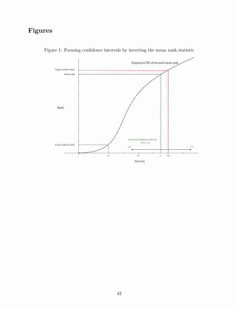
Figures

Figure 1: Forming confidence intervals by inverting the mean rank statistic

-a 0 +b

Elasticity

c

Inverted confidence interval:

c-b c+a

[c-b,c+a]

Mean rank

Upper critical value

Lower critical value

Rank

Empirical CDF of inverted mean rank

43

Figure 2: Quarterly minimum wage changes and usable treatment events during 1979-2013

AKARAZ AZ AZ AZ AZ AZ

CACACACA CA CA CACOCOCOCOCOCOCO

CT CT CT CT CT CT CT CT CT CT CT CTDEDE DEDE DE DE DE

FLFL FL FL FL FLFLFL FLHI HI HI HI

IA IA IA IA IAIL IL

MAMAMA MAMA MA MAMAMD

MEME MEME ME MEMEMEMEMEMEMI

MNMNMN MNMOMOMO MOMT MT MT MT MT MTNC

NDNDNH NH NH NH NH NH

NJ NJNMNM

NVNV NV NVNY NY

OHOHOH OHOHOHOROROROR OROROR OROROROROROR OROROR

PA PARI RI RIRI RIRI RI RI RIRI RI RI

VTVT VT VT VT VT VT VT VT VT VT VT VT VT VT VTWA WAWAWAWAWAWAWAWAWAWAWA WAWAWA

WI WIWIWI

AK

CA CACT

FLHI HI HI

ILMA MA

ME ME

MN MN

NHNJ

NYOR

PARI RIVT VT VT

WA WAWI

WV

$3.10 $3.35 $3.80 $4.25 $4.75 $5.15 $5.85 $6.55 $7.25 = Federal Minimum

1980 1983 1986 1989 1992 1995 1998 2001 2004 2007 2010 2013

AK

CA CACT

FLHI HI

ILMA MAME MEMN MN

NHNJ

NYOR

PARI RIVT VT VTWA WA

WIWV

$3.10 $3.35 $3.80 $4.25 $4.75 $5.15 $5.85 $6.55 $7.25 = Federal Minimum

1980 1983 1986 1989 1992 1995 1998 2001 2004 2007 2010 2013

Notes: The top panel displays all quarterly state-level minimum wage changes during the 1979-2013 period,with vertical lines representing the federal minimum wage changes, where bolded states indicate the firstminimum wage rise of the 29 usable treatment events. The bottom panel shows the pre-treatment (blue)and post-treatment (red) windows of the 29 treatment events, with red circles showing the minimum wageincreases during the post-treatment periods.

44

Figure 3: Mean annualized elasticities, minimum wage changes, and number of donors, bytime

−.5

−.4

−.3

−.2

−.1

0.1

.2.3

.4.5

Empl

oym

ent E

last

icity

(−28,−25) (−24,−21) (−20,−17) (−16,−13) (−12,−9) (−8,−5) (−4,−1) (0,3) (4,7) (8,11)

Quarters since treatment

Mean elasticityHL elasticity95% HL CI

−.7

−.6

−.5

−.4

−.3

−.2

−.1

0.1

.2.3

.4.5

.6.7

Wag

e El

astic

ity

(−28,−25) (−24,−21) (−20,−17) (−16,−13) (−12,−9) (−8,−5) (−4,−1) (0,3) (4,7) (8,11)

Quarters since treatment

Mean elasticityHL elasticity95% HL CI

0.0

5.1

.15

.2

Min

imum

wag

e ch

ange

(per

cent

)

05

1015

2025

3035

Num

ber o

f eve

nts

(−28,−25) (−24,−21) (−20,−17) (−16,−13) (−12,−9) (−8,−5) (−4,−1) (0,3) (4,7) (8,11)

Quarters since treatment

Mean number of eventsMean minimum wage change

45

Figure 4: Event-specific and aggregated elasticities

AK

CA

CACTFL

HIHI

HIILMA

MA

MEME

MN

MN

NH

NJ

NY

OR

PA RI

RI

VT

VT

VTWA

WA

WI

WV

−1.5

−1−.

50

.51

Empl

oym

ent E

last

icity

−.25 0 .25 .5 .75 1 1.25 1.5Wage Elasticity

Mean elasticityHL elasticityUnitary elastic demand

46

Figure 5: Probability density functions for the employment and wage elasticities of donors

0.5

11.

5

−3 −2 −1 0 1 2 3 4 5 6 7 8Donor employment elasticities

DonorsNormal

0.5

11.

5

−3 −2 −1 0 1 2 3 4 5 6 7 8Donor wage elasticities

Notes: The donor employment (wage) elasticity distributions have mean -0.012 (0.012), standard deviation0.452 (0.565), and kurtosis 5.82 (58.37). For each outcome, the illustrated normal distributions have the samemean and variance. Shapiro-Wilk normality test p-values are 0.000 for both outcomes.

47

Figure 6: Cumulative distribution of estimated percentile ranks

Test of the sharp null hypothesis that ÷e

= 0.

K−S p−value = 0.911A−D p−value = 0.843

0.2

.4.6

.81

0 .2 .4 .6 .8 1Employment elasticity percentile ranks

K−S p−value = 0.000A−D p−value = 0.000

0.2

.4.6

.81

0 .2 .4 .6 .8 1Wage elasticity percentile ranks

Test of the sharp null hypothesis that ÷e

= ÷.

K−S p−value = 0.585A−D p−value = 0.897

0.2

.4.6

.81

0 .2 .4 .6 .8 1Employment elasticity percentile ranks

K−S p−value = 0.055A−D p−value = 0.073

0.2

.4.6

.81

0 .2 .4 .6 .8 1Wage elasticity percentile ranks

Notes: The solid line is the cumulative distribution of percentile ranks of the 29 treatment e�ects, and thedashed line is the uniform CDF. P-values are for the Kolmogorov-Smirnov and Anderson-Darling tests ofequality of these two distributions.

48

Figure 7: Employment and wage elasticities, trimming events on pre-treatment match qualityPost-treatment elasticities

−.3

−.2

−.1

0.1

.2

Post−t

reat

men

t Em

ploy

men

t Ela

stic

ity

0 1 2 3 4 5 6 7 8 9 10 11

Number of trimmed events

95% HL CI

HL elasticity

Mean elasticity

0.1

.2.3

.4.5

Post−t

reat

men

t Wag

e El

astic

ity

0 1 2 3 4 5 6 7 8 9 10 11

Number of trimmed events

Pre-treatment elasticities

−.1

−.05

0.0

5.1

Pre−

treat

men

t Em

ploy

men

t Ela

stic

ity

0 1 2 3 4 5 6 7 8 9 10 11

Number of trimmed events

95% HL CI

HL elasticity

Mean elasticity

−.1

−.05

0.0

5.1

Pre−

treat

men

t Wag

e El

astic

ity

0 1 2 3 4 5 6 7 8 9 10 11

Number of trimmed events

Notes: Mean and HL elasticities and confidence intervals re-calculated after successive trimming of N =0, . . . , 11 events with the highest pre-treatment RMSPE for the actually treated state.

49

Tables

Table 1: Event description: window lengths, number of donors, and minimum wage increase

Window length MW increases

Event Pre Post Donors Number Percent

AK 2003q1 16 12 33 1 0.265CA 1988q3 28 6 36 1 0.269CA 2001q1 8 12 39 2 0.174CT 1987q1 20 12 36 3 0.269FL 2005q2 28 8 21 4 0.295HI 1988q1 24 8 36 1 0.149HI 2002q1 16 12 38 2 0.190HI 2006q1 8 6 21 2 0.160IL 2004q1 20 12 29 2 0.262

MA 1986q3 20 12 39 4 0.119MA 2000q1 8 12 40 2 0.286ME 1985q1 12 12 44 3 0.090ME 2002q1 12 12 38 3 0.233MN 1988q1 24 8 36 2 0.149MN 2005q3 28 8 20 2 0.194NH 1987q1 20 12 36 3 0.090NJ 2005q4 28 6 21 2 0.388NY 2005q1 24 10 20 3 0.388OR 2003q1 12 12 33 3 0.115PA 1989q1 28 4 36 2 0.104RI 1986q3 20 12 39 3 0.194RI 2004q1 12 12 31 3 0.154VT 1986q3 20 12 39 4 0.090VT 1995q1 12 6 44 2 0.118VT 2004q1 8 12 32 3 0.160WA 1989q1 28 4 36 1 0.149WA 1994q1 8 10 44 1 0.153WI 2005q2 28 8 21 4 0.262WV 2006q3 32 4 20 1 0.136

Notes: “Pre” and “Post” are the respective pre-treatment and post-treatment windowlengths. Percent minimum wage increase is the percent increase from the pre-treatmentminimum to the maximum post-treatment minimum wage.

50

Table 2: Summary of treatment events for more restrictive window configurations

Minimum Window Number of donors Percent MW change

Pre- Post- Events Treated states Min. Mean Max. Min. Mean Max.

8 4 29 19 20 33.0 44 0.090 0.193 0.3888 8 22 16 20 33.8 44 0.090 0.195 0.3888 12 15 11 29 36.4 44 0.090 0.179 0.28616 4 19 17 20 31.2 39 0.090 0.209 0.38816 8 14 12 20 31.6 39 0.090 0.208 0.38816 12 8 8 29 36.1 39 0.090 0.185 0.26924 4 11 10 20 27.5 36 0.104 0.226 0.38824 8 6 5 20 25.7 36 0.149 0.240 0.38832 4 1 1 20 20.0 20 0.136 0.136 0.136

Notes: Each row describes the subset of all 29 events in Table 1 with at least the specified number ofpre- and post-treatment quarters.

Table 3: Average pre- and post-treatment RMSPE for donors, by model specification

(1) (2) (3) (4)Employment

Pre-treatment 0.0311 0.0401 0.0372 0.0342Post-treatment 0.0477 0.0510 0.0493 0.0466

Wage

Pre-treatment 0.7022 0.7743 0.7563 0.7336Post-treatment 0.7973 0.7872 0.7878 0.7735

Predictors

Quarterly outcomes YAnnualized outcomes Y Y YBoth annualized outcomes Y YIndustry & Other controls Y

Notes: The average RMSPE is the square root of the mean of all donors’ MSPEs across all treatment events,for either the pre- or post-treatment period. Predictor categories are either all quarterly pre-treatment out-comes (Quarterly), annualized pre-treatment outcomes, both annualized employment and wage pre-treatmentoutcomes, or pre-treatment means of industry shares and demographic/labor market variables.

51

Table 4: Donor weights and distance to treated states

Weights per donor

Donor relation to treatment Inside Outside Relative weight

Employment

Same region 0.052 0.026 1.993Same division 0.087 0.028 3.127Within 0 - 500 miles 0.054 0.027 2.004Within 0 - 1000 miles 0.037 0.026 1.393

Wage

Same region 0.048 0.027 1.788Same division 0.068 0.029 2.375Within 0 - 500 miles 0.048 0.028 1.739Within 0 - 1000 miles 0.037 0.026 1.399

Notes: The inside (outside) weight per donor is equal to the sum across all treatment eventsof the weights assigned to donors inside (outside) the specified area, divided by the totalnumber of inside (outside) donors. Relative weight is the ratio of inside-to-outside weightsper donor. Distance in miles is the distance between population-weighted state centroids.

52

Table 5: Employment and wage elasticities, by event

Employment Wages

Event Elasticity Rank 90% CI Elasticity Rank 90% CI

AK 2003q1 –0.035 0.400 (–0.387, 0.319) 0.533 0.971* ( 0.339, 0.882)CA 1988q3 0.198 0.763 (–0.355, 0.526) 0.083 0.711 (–1.615, 0.594)CA 2001q1 –0.200 0.268 (–0.768, 0.398) 0.405 0.951* ( 0.053, 0.678)CT 1987q1 –0.229 0.132 (–0.695, 0.211) 0.342 0.816 (–0.576, 0.871)FL 2005q2 –0.129 0.435 (–0.637, 0.381) 0.095 0.783 (–0.119, 0.310)HI 1988q1 0.185 0.579 (–0.811, 0.758) 0.602 0.842 (–1.736, 1.172)HI 2002q1 0.149 0.775 (–0.415, 0.705) 0.117 0.775 (–0.305, 0.395)HI 2006q1 –0.272 0.217 (–1.107, 0.715) 0.515 0.913 (–0.595, 0.991)IL 2004q1 –0.208 0.194 (–0.522, 0.271) 0.027 0.710 (–0.406, 0.312)

MA 1986q3 –0.015 0.512 (–1.149, 0.998) 1.337 0.951* ( 0.394, 2.060)MA 2000q1 –0.456 0.024* (–0.834,–0.157) 0.215 0.857 (–0.164, 0.505)ME 1985q1 –0.078 0.522 (–1.230, 1.044) 1.113 0.957* ( 0.184, 2.062)ME 2002q1 0.097 0.725 (–0.271, 0.544) 0.152 0.800 (–0.119, 0.355)MN 1988q1 0.369 0.816 (–0.627, 0.942) 0.361 0.789 (–1.978, 0.930)MN 2005q3 –0.089 0.455 (–0.762, 0.750) 0.036 0.636 (–0.328, 0.577)NH 1987q1 0.197 0.605 (–1.198, 1.517) 1.969 0.947 (–0.784, 3.555)NJ 2005q4 –0.071 0.435 (–0.414, 0.315) 0.241 0.957* ( 0.101, 0.444)NY 2005q1 –0.375 0.136 (–0.781, 0.057) 0.109 0.818 (–0.055, 0.252)OR 2003q1 –0.827 0.143 (–1.544, 0.200) 0.310 0.857 (–0.227, 1.189)PA 1989q1 0.257 0.632 (–1.113, 1.368) 0.144 0.632 (–6.674, 1.578)RI 1986q3 0.218 0.707 (–0.479, 0.842) 0.663 0.951* ( 0.083, 1.108)RI 2004q1 –0.051 0.515 (–0.727, 0.679) 0.130 0.758 (–0.399, 0.777)VT 1986q3 0.769 0.854 (–0.742, 2.120) 0.762 0.780 (–0.496, 1.726)VT 1995q1 –0.689 0.087 (–1.310, 0.216) –0.070 0.435 (–1.262, 0.693)VT 2004q1 0.661 0.941 (–0.105, 1.363) 0.713 0.971* ( 0.221, 1.433)WA 1989q1 0.698 0.947 (–0.261, 1.476) 0.237 0.684 (–4.536, 1.241)WA 1994q1 –0.580 0.065 (–1.393, 0.022) –0.188 0.196 (–0.792, 0.211)WI 2005q2 0.038 0.652 (–0.533, 0.613) –0.127 0.174 (–0.367, 0.116)WV 2006q3 –1.199 0.091 (–2.207, 0.166) –0.162 0.364 (–1.118, 0.811)

Notes: * indicates significance at the 10% level using the percentile rank of the elasticity within the event-specificdonor-based placebo distribution. Inverting this rank obtains 90% CIs.

53

Table 6: Employment and wage elasticities, pooled

Hodges-Lehmann

Median elasticity Mean elasticity Mean rank Elasticity 95% CI

Employment –0.051 –0.058 0.470 –0.036 (–0.170, 0.087)Wages 0.237 0.368 0.758*** 0.266 ( 0.169, 0.414)

Notes: Critical values for the mean percentile rank are derived from the mean of 29 uniform distributions.* p < 0.1, ** p < 0.05, *** p < 0.01.

Table 7: Employment and wage confidence intervals, by pre-treatment donor MSPE ratios

Donor states Donor state elasticities Treated state elasticities

MSPE Ratio Number Fraction Min Max SD Kurtosis Mean rank 95% CI

Employment

. 958 1.000 –1.756 1.640 0.418 4.613 0.470 (–0.170, 0.087)20 958 1.000 –1.756 1.640 0.418 4.613 0.470 (–0.170, 0.087)10 950 0.992 –1.756 1.640 0.419 4.608 0.469 (–0.172, 0.087)5 893 0.932 –1.756 1.640 0.418 4.643 0.470 (–0.175, 0.088)2 727 0.759 –1.756 1.640 0.428 4.729 0.489 (–0.170, 0.104)

Wages

. 958 1.000 –1.586 6.817 0.536 41.036 0.758*** ( 0.169, 0.414)20 904 0.944 –1.586 3.351 0.408 12.102 0.770*** ( 0.176, 0.428)10 879 0.918 –1.586 3.351 0.406 12.433 0.773*** ( 0.174, 0.430)5 835 0.872 –1.586 3.351 0.398 13.530 0.771*** ( 0.172, 0.425)2 677 0.707 –1.522 3.351 0.398 15.282 0.752*** ( 0.162, 0.426)

Notes: Rows show results for samples where donors limited to those with donor-to-treated MSPE ratios lessthan X, where X=. indicates the full sample.* p < 0.1, ** p < 0.05, *** p < 0.01.

54

Table 8: Employment and wage elasticities, by minimal window length

Window length Hodges-Lehmann

Pre- Post- Events Mean elasticity Mean rank Elasticity 95% CI

Employment

. 4 29 –0.058 0.470 –0.036 (–0.170, 0.087)

. 6 26 –0.055 0.460 –0.046 (–0.179, 0.070)

. 8 22 –0.027 0.475 –0.039 (–0.182, 0.105)

. 10 17 –0.057 0.442 –0.099 (–0.261, 0.105)

. 12 15 –0.001 0.488 –0.019 (–0.205, 0.160)8 . 29 –0.058 0.470 –0.036 (–0.170, 0.087)12 . 24 –0.034 0.505 0.007 (–0.134, 0.122)16 . 19 0.038 0.533 0.035 (–0.109, 0.172)20 . 17 0.036 0.526 0.032 (–0.128, 0.184)24 . 11 –0.011 0.540 0.035 (–0.140, 0.221)28 . 8 –0.037 0.551 0.040 (–0.161, 0.280)

Wages

. 4 29 0.368 0.758*** 0.266 ( 0.169, 0.414)

. 6 26 0.402 0.781*** 0.272 ( 0.174, 0.430)

. 8 22 0.440 0.786*** 0.288 ( 0.170, 0.489)

. 10 17 0.512 0.827*** 0.354 ( 0.198, 0.554)

. 12 15 0.586 0.870*** 0.428 ( 0.252, 0.633)8 . 29 0.368 0.758*** 0.266 ( 0.169, 0.414)12 . 24 0.375 0.754*** 0.240 ( 0.142, 0.408)16 . 19 0.388 0.752*** 0.252 ( 0.125, 0.458)20 . 17 0.395 0.738*** 0.227 ( 0.104, 0.473)24 . 11 0.147 0.672** 0.158 ( 0.001, 0.310)28 . 8 0.068 0.617 0.108 (–0.091, 0.271)

Notes: Window length of X restricts the events to the subset with a pre- or post-period greater than Xquarters, where X = . is eight pre-treatment or four post-treatment quarters. Critical values for the meanpercentile rank are derived from the mean of appropriate number of uniform distributions.* p < 0.1, ** p < 0.05, *** p < 0.01.

55

Table 9: Employment and wage elasticities, by alternative predictor sets

(1) (2) (3) (4)Employment

Mean elasticity –0.019 0.001 0.037 –0.058Mean rank 0.499 0.506 0.537 0.470HL elasticity –0.001 0.011 0.053 –0.036HL 95% CI (–0.148, 0.143) (–0.163, 0.157) (–0.096, 0.191) (–0.170, 0.087)

Wage

Mean elasticity 0.358 0.448 0.434 0.368Mean rank 0.760*** 0.781*** 0.790*** 0.758***HL elasticity 0.280 0.297 0.314 0.266HL 95% CI ( 0.183, 0.413) ( 0.199, 0.446) ( 0.213, 0.471) ( 0.169, 0.414)

Predictors

Quarterly outcomes YAnnualized outcomes Y Y YBoth annualized outcomes Y YIndustry & Other controls Y

Notes: Predictor categories are either all quarterly pre-treatment outcomes (Quarterly), annualized pre-treatment outcomes, both annualized employment and wage pre-treatment outcomes, or pre-treatment meansof industry shares and demographic/labor market variables.* p < 0.1, ** p < 0.05, *** p < 0.01.

56

Tabl

e10

:A

ltern

ativ

em

etho

dsof

infe

renc

efo

rem

ploy

men

tel

astic

ity

Ran

k-ba

sed

infe

renc

eA

ggre

gate

dem

ploy

men

tel

astic

ity

95%

crit.

valu

es5%

rej.

rate

Type

Poin

tes

timat

e95

%C

I

Met

hod

1:R

ank,

unifo

rmiid

.(0

.395

,0.

605)

0.05

0H

odge

s-Le

hman

n–0

.036

(–0.

170,

0.08

7)M

etho

d2:

Ran

k,di

scre

teiid

.(0

.398

,0.

601)

0.04

3H

odge

s-Le

hman

n–0

.036

(–0.

164,

0.08

0)M

etho

d3:

Ran

k,ra

nd.

infe

renc

e(0

.388

,0.

611)

0.06

6H

odge

s-Le

hman

n–0

.036

(–0.

178,

0.09

4)M

etho

d4:

Elas

ticity

,ran

d.in

fere

nce

--

Mea

n–0

.058

(–0.

197,

0.10

0)

Notes:

The

base

line

met

hod

1as

sum

esm

ean

rank

isdi

strib

uted

asth

em

ean

of29

unifo

rmva

riabl

eson

[0,1

].M

etho

d2

calc

ulat

esth

era

nkas

the

mea

nof

29pe

rcen

tile

rank

susin

gth

eW

eibu

ll-G

umbe

lper

cent

ilera

nkca

lcul

atio

nw

ithth

eap

prop

riate

num

bero

fdon

orst

ates

fore

ach

even

t.M

etho

d3

furt

herr

elax

esth

eas

sum

ptio

nth

atth

era

nksa

rein

depe

nden

tacr

osse

vent

sby

acco

untin

gfo

rthe

dono

rove

rlap

acro

ssev

ents

.In

part

icul

ar,m

etho

d3

uses

ara

ndom

izat

ion

infe

renc

epr

oced

ure

that

perm

utes

stat

eid

entifi

ersr

ando

mly

,and

then

estim

ates

the

dist

ribut

ion

ofm

ean

rank

sof

the

e�ec

tof

the

plac

ebo

law

s.T

hede

tails

for

the

simul

atio

nar

ede

scrib

edin

the

text

.M

etho

d4

cond

ucts

rand

omiz

atio

nin

fere

nce

usin

gth

em

ean

e�ec

t(e

last

icity

)as

oppo

sed

toth

em

ean

rank

;thi

sm

etho

dus

esth

em

ean

of29

dono

rem

ploy

men

tel

astic

ities

,ch

oosin

gon

edo

norp

erev

ent,

for1

mill

ion

itera

tions

.Rej

ectio

nra

tesf

orea

chm

etho

dar

esh

own

whe

nus

ing

the

criti

calv

alue

sfro

mm

etho

d1.

57

Appendix Tables

Table A1: Extrema of the distribution of mean of N uniformly distributed random variables

Percentile

N 0.5 2.5 5.0 95.0 97.5 99.5

1 0.005 0.025 0.050 0.950 0.975 0.9952 0.050 0.111 0.158 0.842 0.888 0.9503 0.103 0.176 0.223 0.777 0.823 0.8964 0.147 0.220 0.261 0.738 0.780 0.8525 0.182 0.249 0.287 0.713 0.751 0.8196 0.206 0.271 0.305 0.694 0.729 0.7937 0.227 0.288 0.320 0.680 0.712 0.7748 0.244 0.301 0.332 0.668 0.699 0.7579 0.258 0.312 0.341 0.658 0.687 0.743

10 0.269 0.322 0.350 0.650 0.678 0.73111 0.280 0.330 0.357 0.643 0.670 0.72012 0.289 0.337 0.363 0.637 0.663 0.71113 0.297 0.344 0.368 0.632 0.656 0.70314 0.304 0.349 0.373 0.627 0.651 0.69615 0.311 0.354 0.377 0.623 0.646 0.68916 0.317 0.359 0.381 0.619 0.641 0.68317 0.322 0.363 0.385 0.615 0.637 0.67918 0.327 0.367 0.388 0.612 0.633 0.67319 0.331 0.370 0.391 0.609 0.630 0.66920 0.335 0.374 0.394 0.606 0.626 0.66521 0.339 0.377 0.396 0.604 0.623 0.66022 0.343 0.379 0.398 0.601 0.620 0.65723 0.346 0.382 0.401 0.599 0.618 0.65424 0.349 0.384 0.403 0.597 0.615 0.65025 0.352 0.387 0.405 0.595 0.613 0.64726 0.355 0.389 0.407 0.593 0.611 0.64527 0.358 0.391 0.408 0.591 0.609 0.64228 0.360 0.393 0.410 0.590 0.607 0.63929 0.363 0.395 0.412 0.588 0.605 0.63730 0.365 0.397 0.413 0.587 0.603 0.635

Notes: Simulated using one million iterations of the mean of N uniformly distributedvariables on [0, 1].

58