pope pope walmart aej applied

7/31/2019 Pope Pope Walmart Aej Applied

http://slidepdf.com/reader/full/pope-pope-walmart-aej-applied 1/36

0

When Walmart Comes to Town: Always Low Housing

Prices? Always? †

Devin G. PopeBooth School of Business

University of Chicago

Jaren C. Pope * Department of Economics

Brigham Young University

May 2012

Abstract

Walmart often faces strong local opposition when trying to build a new store.Opponents often claim that Walmart lowers nearby housing prices. In this study we useover one million housing transactions located near 159 Walmarts that opened between2000 and 2006 to test if the opening of a Walmart does indeed lower housing prices.Using a difference-in-differences specification, our estimates suggest that a new Walmartstore actually increases housing prices by between 2 and 3 percent for houses located

within 0.5 miles of the store and by 1 to 2 percent for houses located between 0.5 and 1mile.

Keywords: Walmart; Housing Prices;

† We thank Emek Basker, Nick Kuminoff, Lars Lefgren, and Arden Pope as well as colleagues at theUniversity of Chicago and Brigham Young University for helpful discussions about this paper. We alsothank Chris Bruegge and Brendan Forster for excellent research assistance on this project. The standarddisclaimer applies.* Devin Pope: Booth School of Business, University of Chicago, 5807 S Woodlawn Ave, Room 310,Chicago, IL 60637. Phone: 773-702-2297; email: [email protected] .Jaren Pope: Department of Economics, Brigham Young University, 180 Faculty Office Building, Provo,UT 84602-2363. Phone: 801-422-2037; email: [email protected] .



1

1. Introduction

One of the most significant changes over the past two decades in the U.S. retail

market is the expansion of large box stores and supercenters. Walmart is the largest of

these rapidly growing retailers and is currently the biggest private employer in the world.

In the United States alone, Walmart currently operates more than 4,400 retail facilities

and employs almost 1.4 million people. 1 Phone surveys suggest that 84% of households

in the U.S. shop at Walmart in a given year with 42% of households reporting to be

regular Walmart shoppers (Pew Research Center, 2005). These surveys also show that

lower-income households are more likely to shop at Walmart than upper-income

households. In fact, Basker, (2005b), Hausman and Leibtag (2007), and Basker and Noel

(2009) have shown that Walmart “Supercenters” that sell groceries offer many identical

food items as other grocers at an average price that is substantially lower than their

competitors. Hausman and Leibtag (2007) also find that these lower prices translate into a

significant increase in consumer surplus.

Despite the consumer benefits from the expansion of supercenters into new

geographic markets, there is often significant opposition and controversy when Walmart

tries to open a new store. One concern of opponents is the impact that a new Walmart

will have on local employment opportunities and wages. There is a small literature that

has analyzed this common concern including Basker (2005a), Hicks (2007a) and

Neumark et al. (2008). The findings of these studies have been mixed with Basker

(2005a) and Hicks (2007a) finding positive effects on employment and/or wages, while

1 These numbers were taken from the August 2011 fact sheet provided on the Walmart website and can befound at http://walmartstores.com/pressroom/factsheets/



2

Neumark et al. (2008) found negative effects. 2 Another primary concern of opponents to

a new Walmart, is the effect it will have on crime, traffic and congestion, noise and light

pollution, the visual aesthetics of the local area, and ultimately the impact that these

externalities will have on local housing prices. 3 However, unlike the academic literature

that surrounds the labor-market effects of Walmart, there has been no peer-reviewed

work that attempts to understand the impact of Walmart on housing prices. 4

In this paper we try to understand if building a new Walmart has a positive or

negative effect on nearby housing prices. Answering this question is important as citizens

and local governments grapple with the economic impacts of allowing Walmart to build a

new store in their jurisdiction. Analyzing housing prices is a particularly useful way to

understand the economic value of a Walmart entering a community. For example, when a

Walmart is built, it generally is not built in isolation. The Walmart store often acts as a

hub that attracts a variety of other businesses, which in turn, can also have impacts on

housing markets. If households value convenient access to the goods and services that

Walmart and these other businesses provide, then the new stores would have a positive

impact on housing prices. However, if Walmart and the businesses that agglomerate

2 The different findings in these studies depend primarily on the identification strategy employed to accountfor the potential endogeneity of the location and timing of Wal-Mart openings. See Basker (2007) andNeumark et al. (2008) for a discussion of these differences.3An example of these concerns can be seen in a document created by the non-profit communityorganization called “Responsible Growth for Northcross.” This group was formed to oppose a Walmartsupercenter being built near the Northcross mall in Austin, Texas. They made a top 10 list for why Walmart

shouldn’t be built in their town. Number two on their list was that “Wal-Marts Lower Prices. Includingyour property value.” The full list can be found athttp://corpethics.org/downloads/northcross_no_walmart.pdf 4 There is a paper on the impact of Walmart on annual property tax collections and commercial propertiesby Hicks (2007b) and a working paper by Vandegrift, Loyer, and Kababik (2011). There is also a small butgrowing literature on the impact of Walmart on a variety of other outcomes outside of labor and housingmarkets. These include poverty rates (Goetz and Swaminathan, 2006), small business activity (Sobel andDean, 2008), obesity (Courtemanche and Carden, 2011), social capital (Goetz and Rupasingha, 2006;Carden et al., 2009a), leisure activities (Carden and Courtemanche, 2009) and traditional values (Carden etal., 2009b).



3

nearby also impose negative externalities such as increased pollution, crime, and traffic,

then this could adversely impact prices of nearby houses. Thus the housing price effect a

priori is ambiguous. Accurately estimating the housing price changes that result from the

building and opening of a Walmart and the agglomeration it spurs may help local

policymakers to better understand if the net effect of a new Walmart is perceived as

beneficial to nearby households. This could in turn provide some economic justification

for a local government to encourage or discourage the building of a Walmart store in its

jurisdiction.

Our analysis of the impact that Walmart has on housing prices utilizes two unique

datasets. The first dataset describes when and where Walmarts opened between 2000 and

2006. The second dataset includes data for more than one million residential housing

transactions that occurred within four miles of 159 Walmarts that opened during this time

period. In contrast to the county-level analyses conducted by most previous work on the

impacts of Walmart, the micro-level nature of our dataset allows us to develop an

identification strategy that can help us to overcome the potential endogeneity of the

location and timing of Walmart openings. More specifically, we employ a difference-in-

differences analysis that compares housing prices before and after a Walmart opens for

areas very close to a newly built Walmart, to areas slightly farther away.

The results from this analysis suggest that a new Walmart store increases nearby

housing prices. Our primary analysis suggests that houses located within 0.5 miles of the

store see increases in their prices of about 2-3 percent when comparing the two and a half

years before the Walmart opened to the two and a half years after the opening. Houses

between 0.5 and 1 mile from the Walmart see an increase of 1-2 percent. It does not



5

positive correlation between shopping centers and housing prices. These studies suggest

that having convenient access to a Walmart might increase housing prices.

On the other hand, the introduction of a Walmart store in a community also has

the potential to lower housing prices through increased local crime, noise and light

pollution, traffic congestion, garbage accumulation, and loss of perceived visual

aesthetics. Several studies have shown that these disamenities are capitalized into

housing prices. For example, Linden and Rockoff (2008) and Pope (2008) have both

recently shown that a discrete change in the risk of a localized crime can have a causal

impact on housing prices, Smith et al. (2002) showed that freeway noise can have a

negative impact on housing prices, and Lim and Missios (1995) showed the negative

impact of landfills on housing prices.

An important question that has not been addressed in the literature is whether or

not the benefits of access to a Walmart outweigh the costs imposed by any negative

externalities that it imposes on the local community when it builds a store. Analyzing

housing prices before and after a Walmart is built in a given locale offers the potential to

test whether or not the benefits of accessibility outweigh the costs of negative

externalities. If one were to see a decrease in housing prices near a Walmart store after it

was built, this might signal that there are significant negative externalities imposed on

landowners and households nearby Walmart. However, if one were to see an increase in

housing prices, this might suggest that the benefits of easy access to Walmart’s lower

prices or the other shopping that naturally agglomerates near a Walmart outweigh any

negative externalities imposed on local residents.



6

There is some evidence that the value of accessibility declines less rapidly across

space than the costs of localized externalities. Li and Brown (1980) provide empirical

evidence to suggest that although proximity to industry and commercial areas impose

negative externalities on nearby houses, this same proximity creates substantial benefits

to households far enough away to avoid the sphere of influence from the negative

externalities. In the next sections we examine the impact of building Walmart stores on

surrounding housing prices to test whether the benefits of accessibility to Walmart

outweigh the costs of negative externalities that Walmart may impose.

3. Data

The analysis relies on two key datasets. The first is data on Walmart stores that

opened over the relevant time frame of our study. The second is data on single family

residential properties in areas where the Walmart stores opened. In this section we

describe each source of data in preparation for our empirical analysis.

3.1 Walmart Data

The Walmart data includes the address and opening dates of regular Walmart

stores and Walmart supercenters in the United States. 5 The original data contain the full

universe of Walmart stores that were built between 1962 and Jan. 31, 2006. However,

because of housing data constraints, we focus on 159 stores that were built between July

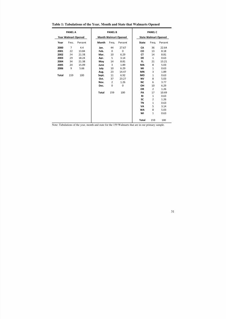
2000 and January 31, 2006 for which we have corresponding housing data. Table 1

5 The data was generously provided to us by Thomas J. Holmes of the University of Minnesota and wasused in his paper, Holmes (2011). The data and additional information on how the data were collected canbe found at Professor Holmes’ website at: http://www.econ.umn.edu/~holmes/research.html



7

provides summary statistics for this dataset over time and space. Panel A shows the years

in which the 159 Walmarts in our primary sample were built. It may seem curious that

there were 9 stores built in 2006 when our dataset ends January 31, 2006. However, Panel

B of Table 1 shows that January is the most common month for Walmarts to open. This is

because January 31 st is considered the end of Walmart's fiscal year and so it appears there

is a push to open new Walmarts before this date. Panel C shows the twenty U.S. states in

our primary sample in which Walmarts were built.

We also collected some additional information on when it was announced that

these Walmarts were to be built. This information was collected using the internet to find

newspaper articles or other online sources that indicated the timing of when the building

of a particular Walmart was announced to the community. After collecting these dates,

we found that the median number of days from when the Walmart store was announced

until its construction was completed and the Walmart store was open for business was

516 days. This information is useful in our analysis to help determine the appropriate size

of the temporal window in which to analyze the housing price effects from a Walmart

opening. The announcement information is also useful for explicitly estimating if there

are price effects from the announcement itself.

3.2 Housing Price Data

Our analysis is based on a large housing dataset of more than one million

observations on the sales of single-family residential properties across the United States

between January 1, 1998 and January 31, 2008. We purchased the data from a

commercial vendor who had assembled them from assessor’s offices in individual towns



8

and counties. 6 The data include the transaction price of each house, the sale date, and a

consistent set of structural characteristics, including square feet of living area, number of

bathrooms, number of bedrooms, year built, and lot size. Using these characteristics, we

performed some standard cleaning of the data, removing outlying observations, removing

houses built prior to 1900, and removing houses built on lots larger than 5 acres.

The data also include the physical address of each house, which we translated into

latitude and longitude coordinates using GIS street maps and a geocoding routine. The

lat-long coordinates were then used to determine the distance of each house to the nearest

Walmart location. In our primary analysis we restrict the data to include only those

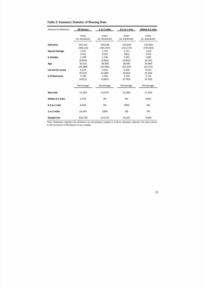
houses that are within four miles of a Walmart and that sold in the two and a half yearsbefore the nearest Walmart opened or in the two and a half years after it opened. 7 Table 2

provides summary statistics of our primary housing dataset. The first column reports the

summary statistics for the over 600,000 housing transactions between 1998 and 2008 that

will be used in our primary analysis. The average sale price, square footage, # of baths,

age, lot size, and number of bedrooms in our full sample of homes was approximately

267,000 dollars, 1,767 square feet, 2 baths, 30 years old, 0.25 acres and 3 bedrooms

respectively. Also, about 15% of houses in our sample of transactions were newly

constructed, approximately 2% are located within 0.5 miles of where a Walmart has or

will be built, 7% are located between 0.5 and 1 mile, and 25% between 1 and 2 miles. 8

The columns labeled “1 to 2 miles”, “0.5 to 1 mile” and “within 0.5 mile” provide

summary statistics for houses within these distances to where a Walmart has or will be

built. The summary statistics indicate that, houses closer to a Walmart tend to be smaller

in size, somewhat newer, and on slightly smaller lots. These small differences in housing

6 The commercial data vendor is Dataquick whose housing data is often used for academic research.7 A four mile radius was chosen a priori following Holmes (2011) assumption that houses within 2 milesare considered within the Walmart’s “neighborhood.” Houses between two and four miles were included inour sample to act as a natural control group.8 A house was defined as new construction if the year it sold was the same year it was reportedly built orthe year after it was built.



9

characteristics suggest that new Walmarts were not built in random locations. The

endogenous placement of Walmarts motivates the empirical strategy that we outline

below.

4. Empirical Strategy

4.1 Hedonic Pricing Method

When a household chooses to purchase a house, it is choosing more than just

housing characteristics; it is also choosing a bundle of locational characteristics such as

school quality, levels of criminal activity, proximity to work, and access to shopping. The

hedonic model was developed by Rosen (1974) to provide a theoretical foundation for the

relationship between prices and attributes. For over 40 years economists have used the

hedonic pricing method in conjunction with the housing market to reveal household

preferences for important locational characteristics. 9

Early work in this area typically used cross-sectional data to try and identify the

implicit price of the locational attribute of focus. The primary concern with this literature

has been the possibility that omitted variables lead to a bias in the estimates for key

implicit prices. For example, if Walmarts tend to be built in areas where there is higher

crime, then a cross-sectional estimate of the implicit price for living near a Walmart that

excludes the relevant measures of crime will be biased downwards (more negative).

Recognizing the importance of mitigating this type of omitted variable bias, a new wave

of hedonic analyses have exploited quasi-experiments in time and/or space to better

overcome omitted variable bias and identify implicit prices of interest. Examples of this

9 Ridker and Henning’s (1967) study on the value of air quality is one of the earliest examples in thisliterature. See Palmquist (2005) for a more complete review of the hedonic method applied to housingmarkets.



11

(1) ijymijijiji jymijym D D DP ε φ θ β α +++++=

20

10

5.00)log( γ X

The log of the sale price of the house is a function of a store ( j) by year ( y) by month ( m)

specific effect ( jymα ), observable individual ( i) property characteristics ( iX ), indicator

variables of individual houses within 0.5, 0.5 to 1, and 1 to 2 miles of a Walmart where

the omitted indicator variable is an indicator for homes between 2 and 4 miles from the

nearest Walmart ( 215.0 ;; ijijij D D D ) and a random error term that allows for year by month

by store area specific correlation in housing prices ( ijymε ). Absent any omitted variable

bias and using only houses that sold after the nearest Walmart was built, estimation of

Equation 1 will yield estimates of the key parameters ( 000ˆ;ˆ;ˆ φ θ β ) that show the impact

that being near a Walmart has on housing prices for homes within 0.5, 0.5 to 1, and 1 to 2

miles of a Walmart relative to homes that are 2 to 4 miles from the store. 11 This

estimation strategy can be considered the “traditional” cross-sectional hedonic approach.

A traditional approach to analyzing the impact that Walmart has on housing prices

may of course be plagued with omitted variable bias. Another hedonic specification that

could be used to help overcome the omitted variable bias would be a spatial difference-

in-differences specification of the following form:

(2)

ijymiymijijijijijiji jymijym Post D D D D D DP ε φ θ β φ θ β α ++++++++= *)()log( 21

11

5.01

20

10

5.00γ X

The key difference between Equation (2) and Equation (1) is that we are exploiting the

timing of the opening of the Walmart. To estimate Equation (2), housing data near a

11 This is of course assuming that the correct functional form is being used as well as other underlyingassumptions for linear regression hold.



12

Walmart both before and after the opening of the Walmart store would be used. The key

parameters in this specification are the estimates for the spatial indicators ( 111ˆ;ˆ;ˆ φ θ β ) that

have been interacted with an indicator for whether the housing transaction took place

after the Walmart was opened ( iymPost ). These parameters give us the local effect on the

treated spatial zones. 12

The key advantage of the difference-in-differences specification is that by

including spatial fixed effects and looking at housing prices before and after the opening

of Walmarts, we can difference away time-invariant omitted variables that could bias our

estimates. However, we must rely on the identifying assumption that housing price trends

for areas near the Walmart and those areas slightly farther away from the Walmart would

have been the same had the Walmart store (and any other stores from the agglomeration

effect) not been built. This assumption would be less attractive if we were using county-

level averages of housing prices to make comparisons between “treated” counties and

“control” counties. As discussed earlier, much of the literature on the labor market effects

relied on county-level measures for their analyses. This is why, for example, Basker

(2005a) and Neumark (2008) relied on instrumental variable strategies to deal with the

endogeneity of Walmart location decisions. In our analysis, instead of needing housing

price trends in treatment and control counties to be the same before and after Walmart is

built, all we need is housing price trends to be the same in the four mile zone surrounding

the Walmart. Given that the area of a circle with a radius of 4 miles is approximately

1/12 th of the area of the median county in the U.S., exploiting the miro-level housing data

12 The estimates generated from this specification are clearly for the houses near the Walmarts in oursample and may not be externally valid, for example, in very rural areas for which we do not have housingtransactions.



14

to 1 mile, or 1 to 2 miles from the nearest Walmart. In the traditional hedonic framework,

the coefficients on these indicators provide information about the marginal willingness to

pay to live near a Walmart store.

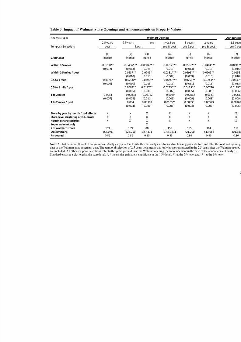
Column (1) in Table 3 provides the coefficients and their standard errors for the

three spatial indicator variables. The standard errors have been clustered at the Walmart

store level. Taken literally, the coefficient on the within 0.5 mile indicator suggests that

Walmarts in our sample reduce the prices of homes within 0.5 miles by approximately

2.5% (statistically significant at the 5% level) and homes between 0.5 and 1 mile by a

little less than 2% (statistically significant at the 10% level). Of course the concern with

interpreting these estimates as the causal impact of Walmart on nearby housing prices is

that they are likely to suffer from omitted variable bias. For example, if Walmart tends to

open stores in areas that are less expensive for unobserved reasons (i.e. lower quality

schools, the local landfill is nearby, further away from downtown, etc.) then these

unobservable disamenities could potentially bias the traditional hedonic coefficients

downwards.

5.2 Difference-in-Differences Results

To help mitigate the concern of omitted variable bias in our analysis we

implement difference-in-differences regressions following Equation (2). The housing

data used in this regression are restricted to houses within four miles of a Walmart that

sold in the two and a half years after (just like in the cross-sectional analysis), but now we

also include houses that sold in the two and a half years before the Walmart was built.

The regression again includes store-by-year-by-month fixed effects and structural



15

characteristics of the house that were described in Table 2. Besides the three spatial

indicator variables that were included in the cross-sectional analysis, interactions of these

indicators with an indicator for the house having sold after the Walmart opened are also

included. The coefficients on these interaction indicators are of primary interest in the

difference-in-differences analysis.

Column (2) in Table 3 provides the coefficients and their standard errors for the

three spatial indicator variables and their interactions with the post-opening indicator

variable. The standard errors have again been clustered at the Walmart store level. The

coefficient on the “within 0.5 miles” indicator suggests that homes within a half mile of

the future Walmart location sold for approximately 5% less than homes two to four miles

away. However, the coefficient on “within 0.5 miles*post” suggests that homes within

0.5 miles of the constructed Walmart store actually sold for approximately 2.5% more

than baseline, after the Walmart was built. In other words, while homes within 0.5 miles

of the future Walmart location sold for 5% less than homes 2 to 4 miles away, they only

sold for 2.5% less after the Walmart was built. Similarly homes between 0.5 and 1 mile

of the future Walmart sold for approximately 3% less before the Walmart, but

experienced an increase in sales prices of approximately one percentage point after the

Walmart was built. Homes between 1 and 2 miles experience a small, but statistically

insignificant increase in housing prices after the Walmart opening relative to the 2 to 4

mile control band.

Column (3) of Table 3 performs a heterogeneity check on our key findings in

Column (2) by focusing the analysis on the 88 Walmart “supercenters” in our sample. 14.

14 A Walmart supercenter is typically larger than a regular Walmart store and also sells grocery items.



16

The magnitude of the coefficient on the indicator “within 0.5 miles*post” is

approximately the same in column (2). The biggest difference is that the coefficient on

“0.5 to 1 mile*post” is twice as large as before suggesting that Walmart supercenters

increase housing prices by approximately 2% for homes between one half and one mile

after a Walmart supercenter opens.

Our Analysis thus far has been using a window of two and a half years before

and after a Walmart opens for the inclusion of housing data in the regressions. In an ideal

quasi-experiment for Walmart openings, the building of a Walmart would be announced

one day and then the next day it would be built and operating. With this sharp

discontinuity in time, one could potentially narrow the temporal window to something

less than two and a half years before and after the opening of the nearest Walmart.

However, the Walmarts in our sample took approximately one and a half years on

average to be built after they were publicly announced. Therefore if there is some change

in housing prices due to the announcement rather than the opening, narrowing the

temporal window would cause the estimates to be attenuated. On the other hand, if we

allow the temporal window to be very large, then we would be forced to drop many

Walmarts from our sample since we analyze only Walmarts that have enough housing

data around the opening date to create a symmetric temporal window. Since we only have

housing data from 1998 to 2008 available to us, requiring five years of pre-opening

housing data and five years of post-opening housing data would only allow us to use

Walmart’s that were built in 2003. Thus two and a half years was chosen to balance the

tradeoff between excluding too many Walmarts and including enough housing sales that



17

occurred before the announcement of the Walmart in an effort to mitigate the attenuation

that may occur from the announcement effect.

Although from an experimental perspective it is nice to keep the temporal window

for the inclusion of housing data symmetric around the Walmart opening date, one could

potentially relax this to include Walmart stores in the analysis that have at least two and a

half years of housing data before and after the opening, but then include housing

observations that were temporally more distant than two and a half years before or after

the opening. Column (4) shows the results of this difference-in-differences specification

that does not exclude housing observations that are temporally more distant than two and

a half years before or after the nearest Walmart’s opening. The key coefficients are

slightly larger with the within 0.5 mile*post coefficient suggesting an approximate 3.3

percent increase in housing prices and the 0.5 to 1 mile*post coefficient suggesting an

approximate 2.3 percent increase.

One could also potentially widen or narrow the temporal window to check for

robustness. Column (5) in Table 3 redoes the difference-in-differences analysis but

widens the temporal window to include three years of housing data pre and post Walmart

opening, while Column (6) narrows the temporal window to include only two years of

housing data pre and post. The main findings are robust to these changes in the temporal

window. The size of the coefficient on the “within 0.5 mile*post” indicator is slightly

larger than in column (2) when the window is expanded to three years before and after,

and slightly smaller when contracted to two years before and after. This is consistent with

our earlier conjecture that if there is some change in housing prices due to the



18

announcement or construction of the Walmart prior to the opening, narrowing the

temporal window would cause the estimates to be attenuated downwards.

We can also more formally analyze whether or not there is an announcement

effect on housing prices by applying our difference-in-differences analysis to the

announcement date rather than the opening date. This time we include the housing data

covering the two and a half years before and after the Walmart is announced . Column (7)

of Table 3 shows the results of this analysis. The coefficient on “within 0.5 miles” shows

once again that homes within a half mile of the future Walmart location sold for

approximately 5% less than homes two to four miles away. The interaction of the post-

Walmart opening indicator for this distance suggests a 1.6% increase in housing prices

although it is not statistically significant using conventional measures. The “0.5 to 1

mile*post” coefficient suggests an approximate 1.4% increase in housing prices in the

year after the announcement in this spatial zone and this result is statistically significant

at the 5 percent level. These results are suggestive of there being some impact even from

the announcement of the Walmart.

5.3 Housing Composition Effects

One issue with how we interpret the results we have found, has to do with

whether or not the types of houses that are selling after a Walmart is built (or announced)

are substantially different than the types of houses that were being sold previously. If

there is a large compositional difference in the types of houses that transacted before and

after, then this may signal that the housing price effects we observe are being at least

partially driven by supply rather than demand. To be clear, this is still an impact of the



19

Walmart being built (or announced), but it suggests that the estimates are not as tightly

linked to household preferences and their perceptions about local externalities and the

benefits of accessibility to shopping.

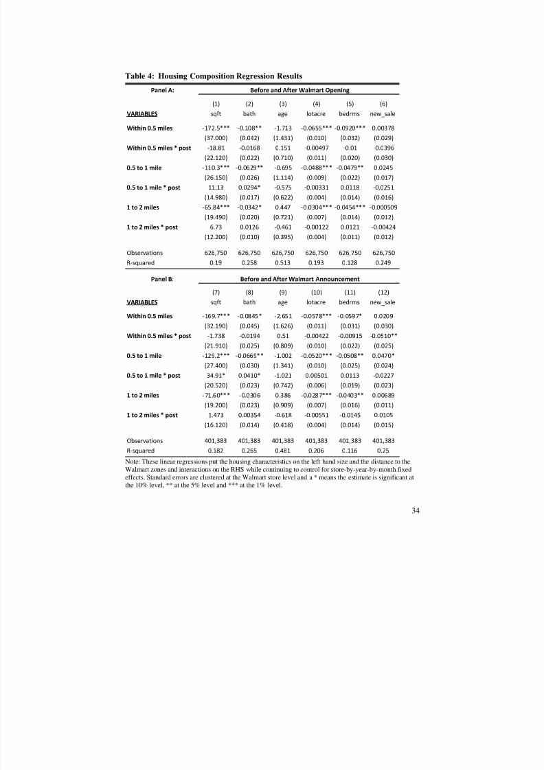
To explore the composition effects in this application, we ran a series of linear

regressions with our key housing attributes on the left hand side and the distance to

Walmart zone indicators and interactions on the right hand side. In these regressions we

continued to control for store-by-year-by-month fixed effects and clustered the standard

errors at the Walmart store level. Once again, the coefficients on the Walmart zone

indicators interacted with the “post” time period are of primary interest as they will signal

if there were substantial changes in these housing characteristics after the Walmart was

built (or announced). Table 4 provides the results from these regressions. Panel A shows

the results where we analyze changes in structural characteristics before and after

Walmart opened , and Panel B shows the results where we analyze changes in structural

characteristics before and after Walmart was announced . Of the 18 interaction

coefficients that are estimated in Panel A, only one is statistically significant (at the 10%

level) suggesting there was no substantial housing composition change before and after

Walmart opened. Of the 18 interaction coefficients estimated in Panel B, 3 are

statistically significant at the 10% level but only 1 of those is significant at the 5% level.

This lone coefficient suggests that there was an approximate 5% decrease in new houses

that were sold after the Walmart was announced in the 0 to 0.5 mile zone. Overall, these

regressions do not seem consistent with strong housing composition effects before and

after either a Walmart’s opening or announcement.



20

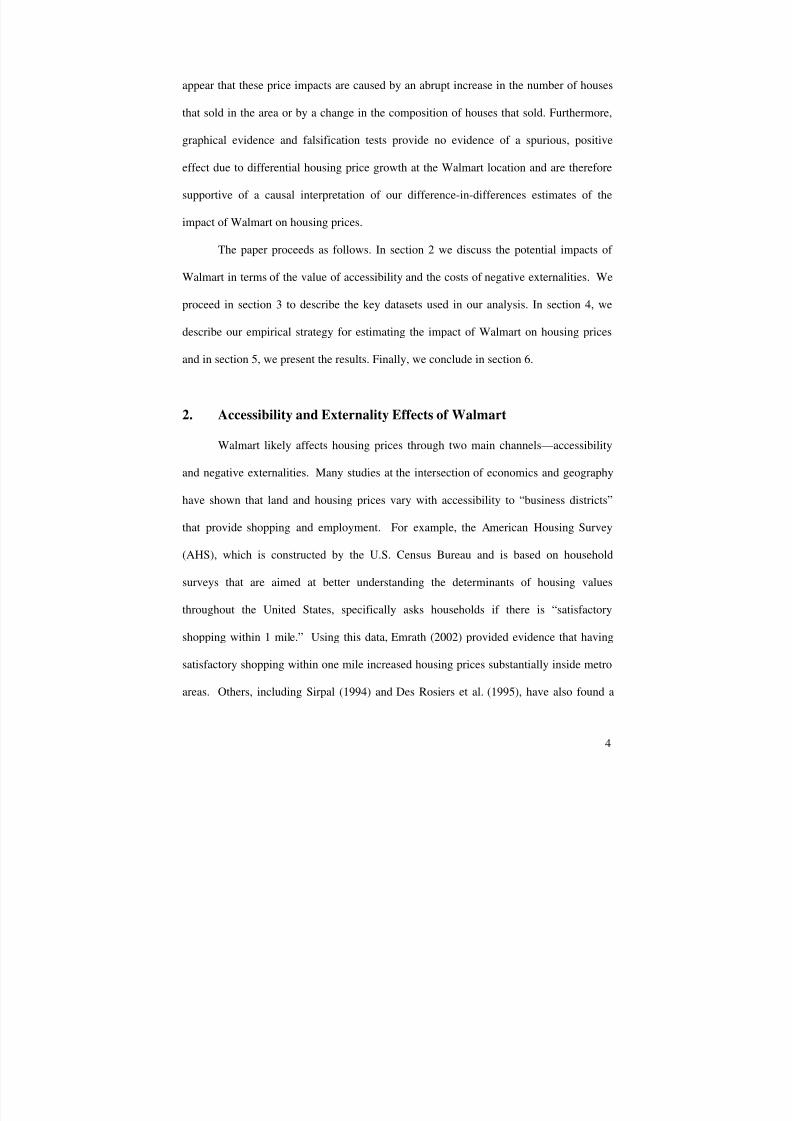
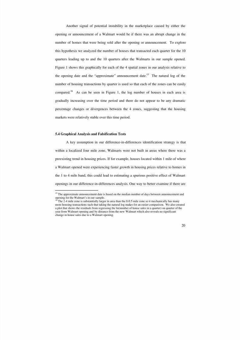
Another signal of potential instability in the marketplace caused by either the

opening or announcement of a Walmart would be if there was an abrupt change in the

number of homes that were being sold after the opening or announcement. To explore

this hypothesis we analyzed the number of houses that transacted each quarter for the 10

quarters leading up to and the 10 quarters after the Walmarts in our sample opened.

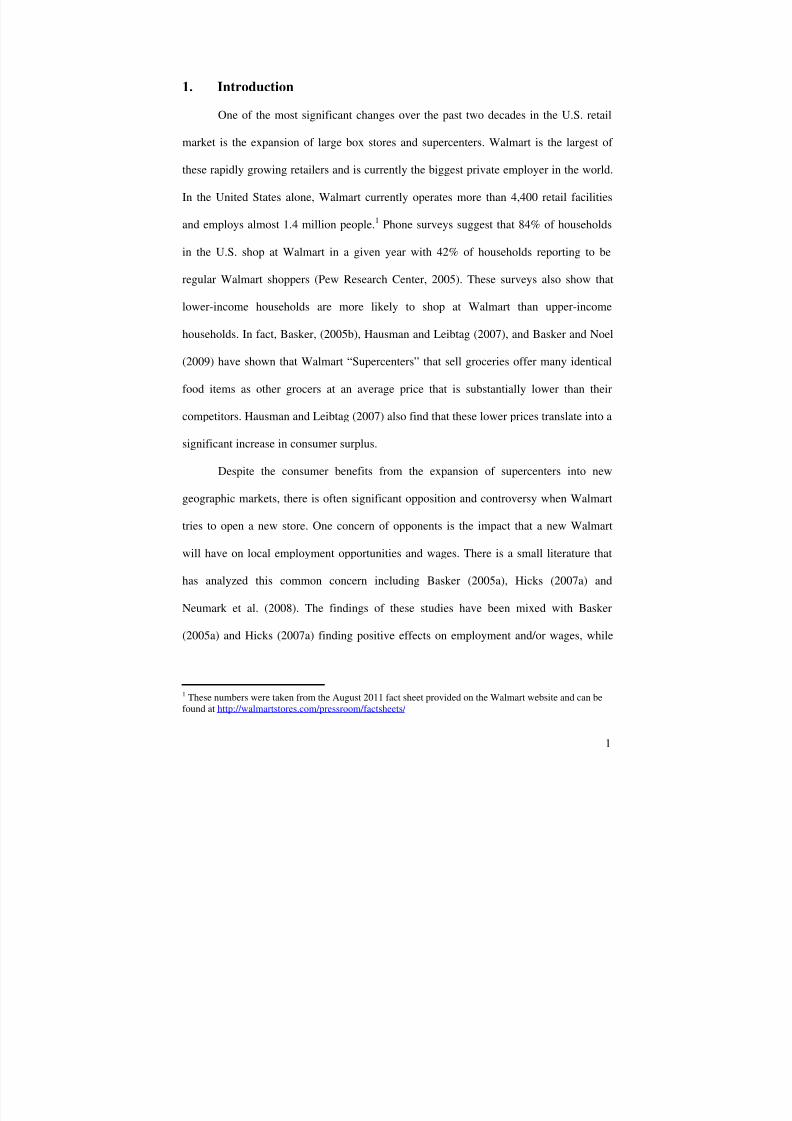
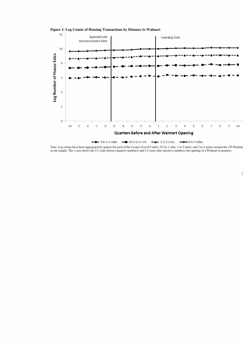
Figure 1 shows this graphically for each of the 4 spatial zones in our analysis relative to

the opening date and the “approximate” announcement date. 15 The natural log of the

number of housing transactions by quarter is used so that each of the zones can be easily

compared. 16 As can be seen in Figure 1, the log number of houses in each area is

gradually increasing over the time period and there do not appear to be any dramatic

percentage changes or divergences between the 4 zones, suggesting that the housing

markets were relatively stable over this time period.

5.4 Graphical Analysis and Falsification Tests

A key assumption in our difference-in-differences identification strategy is that

within a localized four mile zone, Walmarts were not built in areas where there was a

preexisting trend in housing prices. If for example, houses located within 1 mile of where

a Walmart opened were experiencing faster growth in housing prices relative to homes in

the 1 to 4 mile band, this could lead to estimating a spurious positive effect of Walmart

openings in our difference-in-differences analysis. One way to better examine if there are

15 The approximate announcement date is based on the median number of days between announcement andopening for the Walmart’s in our sample.16 The 2-4 mile zone is substantially larger in area than the 0-0.5 mile zone so it mechanically has manymore housing transactions such that taking the natural log makes for an easier comparison. We also createda plot that shows the residuals from regressing the ln(number of house sales in a quarter) on quarter of theyear from Walmart opening and by distance from the new Walmart which also reveals no significantchange in house sales due to a Walmart opening.



21

preexisting trends in the housing prices near where Walmart stores are built is to

graphically illustrate housing price trends in the spatial zones before and after Walmart

opens.

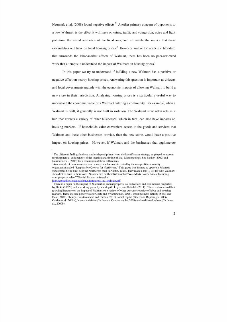
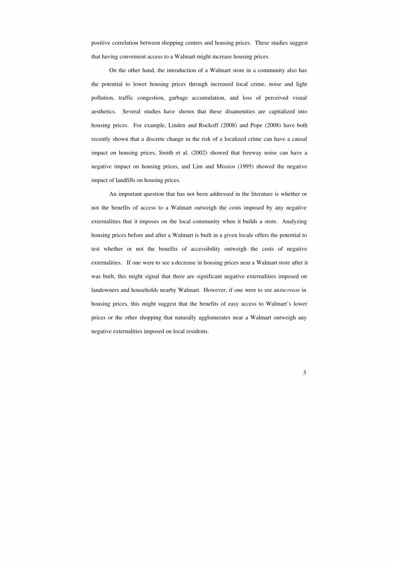
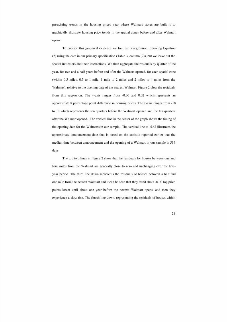
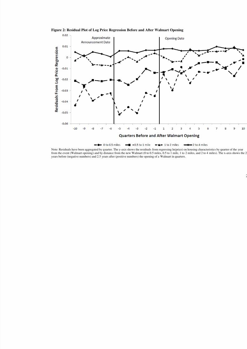
To provide this graphical evidence we first run a regression following Equation

(2) using the data in our primary specification (Table 3, column (2)), but we leave out the

spatial indicators and their interactions. We then aggregate the residuals by quarter of the

year, for two and a half years before and after the Walmart opened, for each spatial zone

(within 0.5 miles, 0.5 to 1 mile, 1 mile to 2 miles and 2 miles to 4 miles from the

Walmart), relative to the opening date of the nearest Walmart. Figure 2 plots the residuals

from this regression. The y-axis ranges from -0.06 and 0.02 which represents an

approximate 8 percentage point difference in housing prices. The x-axis ranges from -10

to 10 which represents the ten quarters before the Walmart opened and the ten quarters

after the Walmart opened. The vertical line in the center of the graph shows the timing of

the opening date for the Walmarts in our sample. The vertical line at -5.67 illustrates the

approximate announcement date that is based on the statistic reported earlier that the

median time between announcement and the opening of a Walmart in our sample is 516

days.

The top two lines in Figure 2 show that the residuals for houses between one and

four miles from the Walmart are generally close to zero and unchanging over the five-

year period. The third line down represents the residuals of houses between a half and

one mile from the nearest Walmart and it can be seen that they trend about -0.02 log price

points lower until about one year before the nearest Walmart opens, and then they

experience a slow rise. The fourth line down, representing the residuals of houses within



22

0.5 miles of the Walmart, shows the most dramatic change from before and after the

Walmart opens. The residuals start out around -0.04 until about one year before the

Walmart opens and then there appears to be a dramatic increase in the residuals until they

are near zero, two and a half years after the Walmart opens. Overall the residuals for the

four zones are “fanned out” before the Walmart opens, are relatively steady until a year

before the Walmart opens, and then they compress until they are nearly identical two and

a half years after the Walmart opens. Given that it is likely to be apparent to homebuyers

that a Walmart is being built two or three quarters before it is complete, this graphical

evidence bolsters the argument that our difference-in-differences estimates are causal.

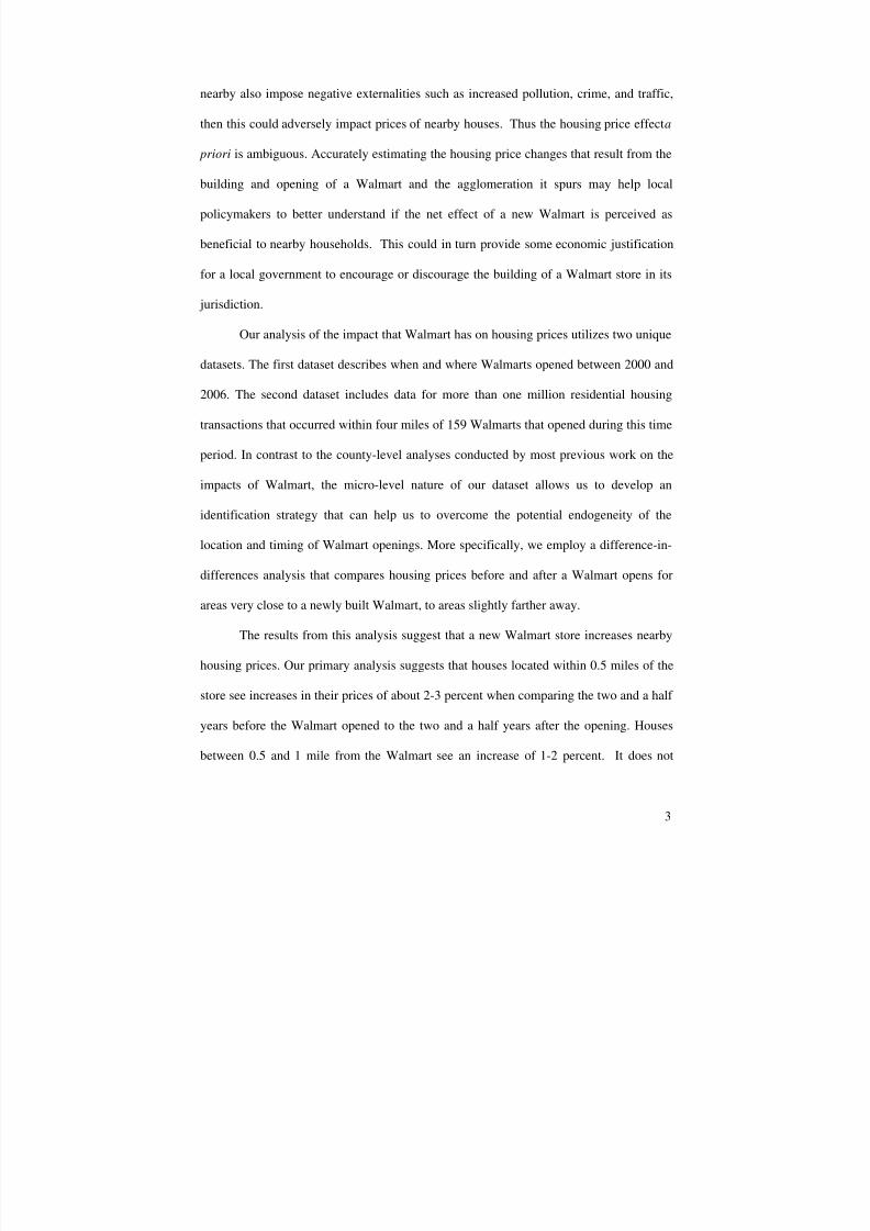
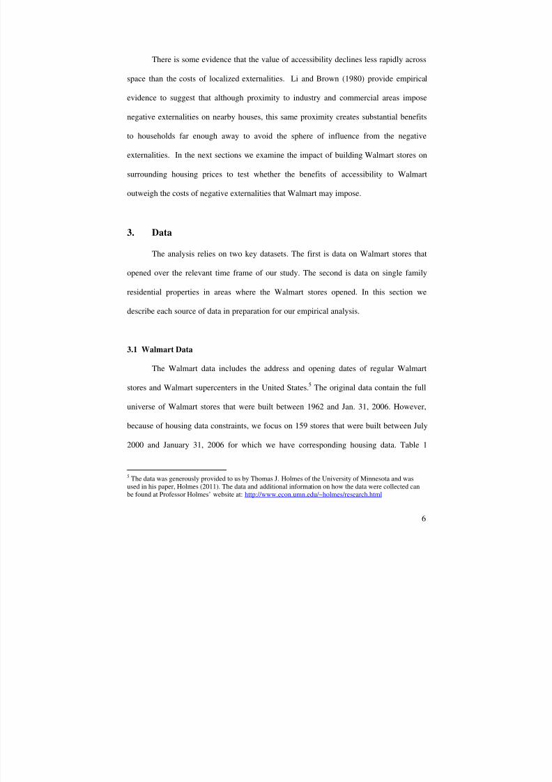
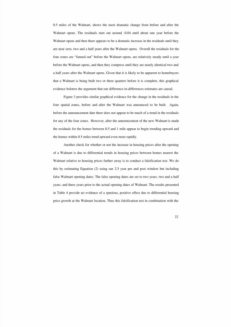
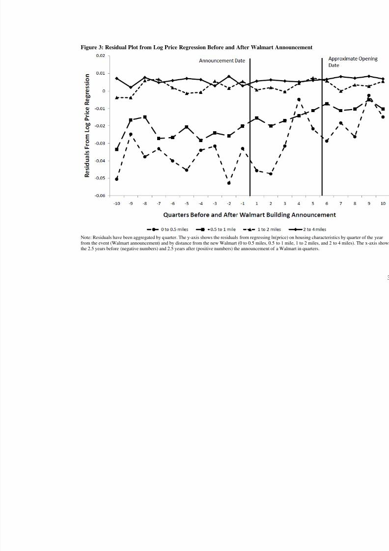
Figure 3 provides similar graphical evidence for the change in the residuals in the

four spatial zones, before and after the Walmart was announced to be built. Again,

before the announcement date there does not appear to be much of a trend in the residuals

for any of the four zones. However, after the announcement of the new Walmart is made

the residuals for the homes between 0.5 and 1 mile appear to begin trending upward and

the homes within 0.5 miles trend upward even more rapidly.

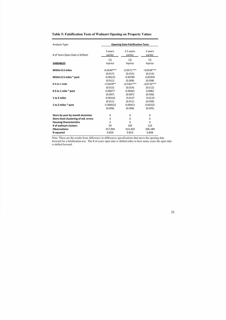
Another check for whether or not the increase in housing prices after the opening

of a Walmart is due to differential trends in housing prices between homes nearest the

Walmart relative to housing prices farther away is to conduct a falsification test. We do

this by estimating Equation (2) using our 2.5 year pre and post window but including

false Walmart opening dates. The false opening dates are set to two years, two and a half

years, and three years prior to the actual opening dates of Walmart. The results presented

in Table 4 provide no evidence of a spurious, positive effect due to differential housing

price growth at the Walmart location. Thus this falsification test in combination with the



23

graphical analysis is supportive of a causal interpretation of our difference-in-differences

estimates of the impact of Walmart on housing prices.

6. Conclusion

Although recent academic work has made it clear that the opening of a Walmart

lowers retail prices for consumers in the area, there has been little work that

systematically tests whether or not the opening of a Walmart lowers housing prices. In

this paper we have attempted to answer this question. We compiled a unique dataset that

linked micro-level housing data to 159 Walmarts that opened in the United States

between 2000 and 2006. Exploiting the spatial resolution of the data we compared areas

very near the Walmarts to areas slightly further away before and after the Walmarts

opened. The results from our primary difference-in-differences specification suggest that

a new Walmart store actually increases housing prices by between 2 and 3 percent for

houses located within a half mile of the store and by 1 to 2 percent for houses located

between a half and one mile from the store. For the average priced home in these areas

this translates into an approximate $7,000 increase in housing price for homes within a

half mile of a newly opened Walmart and a $4,000 increase for homes between a half and

one mile.

Overall, the estimated capitalization effects that we find suggest a revealed

preference by many households to live near a Walmart and the stores that naturally

agglomerate nearby. On average, the benefits to quick and easy access to the lower retail

prices offered by Walmart and shopping at these other stores appear to matter more to

households than any increase in crime, traffic and congestion, noise and light pollution,



24

or other negative externalities that would be capitalized into housing prices. This result is

useful to policymakers that consider passing zoning regulations and other laws that could

affect Walmart’s ability to build new stores within their jurisdiction.

Although we in general find the results to be reasonably credible, some caveats

should also be made. It is possible that while the accessibility benefits appear to extend

out to at least a mile, there may still be negative externalities that affect households that

live very close to a Walmart. Furthermore, our findings provide evidence that Walmarts

increase housing values on average , but it is possible that in certain cases a new store

may actually decrease housing values due to externalities. Finally, our estimates may be

internally valid, but they may not be accurate in more rural areas, for example, where we

do not have housing data. Examining the housing price impacts of Walmart in these

other settings may be important to policymakers and could be looked at in future

research.



25

References

Basker, E. (2005a). "Job creation or destruction? Labor-market effects of Wal-Martexpansion. " Review of Economics and Statistics 87 : 174-183.

Basker, E. (2005b). "Selling a cheaper mousetrap: Wal-Mart’s effect on retail prices."Journal of Urban Economics 58 : 203-229.

Basker, E. (2007). "The causes and consequences of Wal-Mart’s growth." Journal of Economic Perspectives 21 : 177-198.

Basker, E. and M. Noel (2009). "The evolving food chain: competitive effects of Wal-Mart’s entry into the supermarket industry." Journal of Economics andManagement Strategy 18(4) : 977-1009.

Black, S. (1999). "Do Better Schools Matter? Parental Valuation of ElementaryEducation." Quarterly Journal of Economics 114 (2): 577-599.

Carden, A. and C. Courtemanche (2009). "Wal-Mart, leisure, and culture." ContemporaryEconomic Policy 27 : 450-460.

Carden, A., C. Courtemanche and J. Meiners (2009a). "Does Wal-Mart reduce socialcapital?" Public Choice 138 : 109-136.

Carden, A., C. Courtemanche and J. Meiners (2009b). "Painting the Town Red? Wal-Mart and Values." Business and Politics 11 (Article 5).

Chay, K. and M. Greenstone (2005). "Does Air Quality Matter? Evidence from theHousing Market." Journal of Political Economy 113 (2): 376-424.

Des Rosiers, F, A. Lagana, and . (1995). "Shopping centres and house values: anempirical investigation." Journal of Property Valuation and Investment January,2002: 9-13.

Des Rosiers, F., A. Lagana, M. Thériault and M. Beaudoin (1996). "Shopping centresand house values: an empirical investigation." Journal of Property Valuation andInvestment 14( 4): 41-62.

Emrath, P. (2002). "Explaining Housing Prices." Housing Economics January, 2002 : 9-13.

Figlio, D. N. and M. E. Lucas (2004). "What’s in a Grade? School Report Cards and theHousing Market." American Economic Review 94 (3): 591-604.

Goetz, S. and A. Rupasingha (2006). "Wal-Mart and social capital." American Journal of Agricultural Economics 88 : 1304-1310.



Figure 1: Log Counts of Housing Transactions by Distance to Walmart

Note: Log counts have been aggregated by quarter for each of the 4 zones (0 to 0.5 miles, 0.5 to 1 mile, 1 to 2 miles, and 2 to 4 miles) aroin our sample. The x-axis shows the 2.5 years before (negative numbers) and 2.5 years after (positive numbers) the opening of a Walmart



Figure 2: Residual Plot of Log Price Regression Before and After Walmart Opening

Note: Residuals have been aggregated by quarter. The y-axis shows the residuals from regressing ln(price) on housing characteristics by qfrom the event (Walmart opening) and by distance from the new Walmart (0 to 0.5 miles, 0.5 to 1 mile, 1 to 2 miles, and 2 to 4 miles). Thyears before (negative numbers) and 2.5 years after (positive numbers) the opening of a Walmart in quarters.



Figure 3: Residual Plot from Log Price Regression Before and After Walmart Announcement

Note: Residuals have been aggregated by quarter. The y-axis shows the residuals from regressing ln(price) on housing characteristics by qfrom the event (Walmart announcement) and by distance from the new Walmart (0 to 0.5 miles, 0.5 to 1 mile, 1 to 2 miles, and 2 to 4 milethe 2.5 years before (negative numbers) and 2.5 years after (positive numbers) the announcement of a Walmart in quarters.



31

Table 1: Tabulations of the Year, Month and State that Walmarts Opened

Year Freq. Percent Month Freq. Percent State Freq. Percent2000 7 4.4 Jan. 44 27.67 CA 36 22.642001 22 13.84 Feb. 0 0 CO 13 8.182002 34 21.38 Mar. 10 6.29 CT 14 8.812003 29 18.24 Apr. 5 3.14 DE 1 0.632004 34 21.38 May 14 8.81 FL 21 13.212005 24 15.09 June 3 1.89 MA 8 5.032006 9 5.66 July 10 6.29 MI 1 0.63

Aug. 23 14.47 MN 3 1.89Total 159 100 Sept. 11 6.92 MO 1 0.63

Oct. 37 23.27 NV 8 5.03Nov. 2 1.26 NC 6 3.77

Dec. 0 0 OH 10 6.29OR 2 1.26

Total 159 100 PA 17 10.69RI 1 0.63SC 2 1.26TN 1 0.63VA 5 3.14WA 8 5.03WI 1 0.63

Total 159 100

Year Walmart Opened Month Walmart Opened State Walmart Opened

PANEL BPANEL A PANEL C

Note: Tabulations of the year, month and state for the 159 Walmarts that are in our primary sample.



32

Table 2: Summary Statistics of Housing Data

Distance to Walmart: All Houses 1 to 2 miles 0.5 to 1 mile Within 0.5 mile

mean mean mean mean

(st. deviation) (st. deviation) (st. deviation) (st. deviation)

Sale price 267,423 263,628 253,039 237,924(188,323) (181,397) (161,573) (145,603)

Square footage 1,767 1,742 1,721 1,625(743) (720) (681) (593)

# of baths 2.198 2.196 2.201 2.087(0.854) (0.856) (0.832) (0.759)

Age 30.116 30.300 28.487 29.069(25.480) (25.936) (25.222) (24.312)

Lot size (in acres) 0.254 0.242 0.226 0.213(0.327) (0.285) (0.262) (0.236)

# of Bedrooms 3.198 3.186 3.199 3.134(0.811) (0.807) (0.783) (0.756)

Percentage Percentage Percentage Percentage

New Sale 15.29% 15.07% 16.28% 11.70%

Within 0.5 miles 1.57% 0% 0% 100%

0.5 to 1 mile 6.64% 0% 100% 0%

1 to 2 miles 24.54% 100% 0% 0%

Sample size 626,750 153,775 41,622 9,826 Note: Summary statistics for all houses in our primary sample as well as summary statistics for areas closerto the locations of Walmarts in our sample.



Table 3: Impact of Walmart Store Openings and Announcements on Property Values

Analysis Type:

Temporal Selection:

2.5 years

post

>=2.5 yrs

pre & post

3 years

pre & post

(1) (2) (3) (4) (5) VARIABLES lnprice lnprice lnprice lnprice lnprice lnp

Within 0.5 miles -0.0260** -0.0486*** -0.0504*** -0.0512*** -0.0502*** -0.0484*(0.012) (0.013) (0.015) (0.013) (0.013) (0

Within 0.5 miles * post 0.0237** 0.0249* 0.0331*** 0.0296*** 0.020(0.010) (0.013) (0.009) (0.009) (0

0.5 to 1 mile -0.0178* -0.0268** -0.0295** -0.0299*** -0.0255** -0.024(0.009) (0.010) (0.015) (0.011) (0.011) (0

0.5 to 1 mile * post 0.00942* 0.0187** 0.0233*** 0.0125** 0.00

(0.005) (0.008) (0.007) (0.005) (01 to 2 miles -0.0051 -0.00878 -0.00712 -0.0089 -0.00812 -0.0(0.007) (0.008) (0.011) (0.009) (0.009) (0

1 to 2 miles * post 0.004 0.00368 0.0103** 0.00535 0.0(0.004) (0.006) (0.005) (0.004) (0

Store by year by month fixed effects X X X X X Store-level clustering of std. errors X X X X X Housing characteristics X X` X X X Super walmart only X# of walmart stores 159 159 88 159 155 Observations 358,076 626,750 347,371 1,481,811 721,200 513,R-squared 0.86 0.86 0.85 0.85 0.86

Walmart Opening

2.5 years pre

& post

Note: All but column (1) are DID regressions. Analysis type refers to whether the analysis is focused on housing prices before and after tdate or the Walmart announcement date. The temporal selection of 2.5 years post means that only houses transacted in the 2.5 years after are included. All other temporal selections refer to the years pre and post the Walmart opening (or announcement in the case of the annouStandard errors are clustered at the store level. A * means the estimate is significant at the 10% level, ** at the 5% level and *** at the 1%



34

Table 4: Housing Composition Regression Results

Panel A:

(1) (2) (3) (4) (5) (6)VARIABLES sqft bath age lotacre bedrms new_sale

Within 0.5 miles -172.5*** -0.108** -1.713 -0.0655*** -0.0920*** 0.00378

(37.000) (0.042) (1.431) (0.010) (0.032) (0.029)

Within 0.5 miles * post -18.81 -0.0168 0.151 -0.00497 -0.01 -0.0396

(22.120) (0.022) (0.710) (0.011) (0.020) (0.030)

0.5 to 1 mile -110.3*** -0.0629** -0.695 -0.0488*** -0.0479** 0.0245

(26.150) (0.026) (1.114) (0.009) (0.022) (0.017)

0.5 to 1 mile * post 11.13 0.0294* -0.575 -0.00331 0.0118 -0.0251

(14.980) (0.017) (0.622) (0.004) (0.014) (0.016)

1 to 2 miles -65.84*** -0.0342* 0.447 -0.0304*** -0.0454*** -0.000509(19.490) (0.020) (0.721) (0.007) (0.014) (0.012)

1 to 2 miles * post 6.73 0.0126 -0.461 -0.00122 0.0121 -0.00424

(12.200) (0.010) (0.395) (0.004) (0.011) (0.012)

Observations 626,750 626,750 626,750 626,750 626,750 626,750

R-squared 0.19 0.258 0.513 0.193 0.128 0.249

Panel B:

(7) (8) (9) (10) (11) (12)

VARIABLES sqft bath age lotacre bedrms new_sale

Within 0.5 miles -169.7*** -0.0845* -2.651 -0.0578*** -0.0597* 0.0209

(32.190) (0.045) (1.626) (0.011) (0.031) (0.030)

Within 0.5 miles * post -1.738 -0.0194 0.51 -0.00422 -0.00915 -0.0510**

(21.910) (0.025) (0.809) (0.010) (0.022) (0.025)

0.5 to 1 mile -129.2*** -0.0669** -1.002 -0.0520*** -0.0508** 0.0470*

(27.400) (0.030) (1.341) (0.010) (0.025) (0.024)

0.5 to 1 mile * post 34.91* 0.0410* -1.021 0.00501 0.0113 -0.0227

(20.520) (0.023) (0.742) (0.006) (0.019) (0.023)

1 to 2 miles -71.60*** -0.0306 0.386 -0.0287*** -0.0403** 0.00689

(19.200) (0.023) (0.909) (0.007) (0.016) (0.011)

1 to 2 miles * post 1.473 0.00354 -0.618 -0.00551 -0.0145 0.0105(16.120) (0.014) (0.418) (0.004) (0.014) (0.015)

Observations 401,383 401,383 401,383 401,383 401,383 401,383

R-squared 0.182 0.265 0.481 0.206 0.116 0.25

Before and After Walmart Opening

Before and After Walmart Announcement

Note: These linear regressions put the housing characteristics on the left hand size and the distance to theWalmart zones and interactions on the RHS while continuing to control for store-by-year-by-month fixedeffects. Standard errors are clustered at the Walmart store level and a * means the estimate is significant atthe 10% level, ** at the 5% level and *** at the 1% level.



Table 5: Falsification Tests of Walmart Opening on Property Values

Analysis Type:

# of Years Open Date is Shifted:3 yearsearlier

2.5 yearsearlier

2 yearsearlier

(1) (2) (3)VARIABLES lnprice lnprice lnprice

Within 0.5 miles -0.0540*** -0.0571*** -0.0504***(0.017) (0.015) (0.014)

Within 0.5 miles * post -0.00222 0.00785 0.00959(0.011) (0.009) (0.008)

0.5 to 1 mile -0.0398** -0.0363*** -0.0333***(0.015) (0.014) (0.012)

0.5 to 1 mile * post 0.00677 0.00461 0.0082(0.007) (0.007) (0.006)

1 to 2 miles -0.00162 -0.0127 -0.0119(0.011) (0.011) (0.009)

1 to 2 miles * post -0.000522 0.00413 0.00325(0.006) (0.006) (0.005)

Store by year by month dummies X X XStore-level clustering of std. errors X X XHousing Characteristics X X X# of walmart clusters 90 105 123

Observations 257,904 314,302 396,289R-squared 0.859 0.853 0.848

Opening Date Falsification Tests

Note: These are the results from difference-in-differences specifications that move the opening dateforward for a falsification test. The # of years open date is shifted refers to how many years the open dateis shifted forward.

pope pope walmart aej applied

Documents