University of Arkansas, FayettevilleScholarWorks@UARK

Theses and Dissertations

5-2015

Population Dynamics in Active Galactic NucleiJon BesslerUniversity of Arkansas, Fayetteville

Follow this and additional works at: http://scholarworks.uark.edu/etd

Part of the External Galaxies Commons, and the Stars, Interstellar Medium and the GalaxyCommons

This Thesis is brought to you for free and open access by ScholarWorks@UARK. It has been accepted for inclusion in Theses and Dissertations by anauthorized administrator of ScholarWorks@UARK. For more information, please contact scholar@uark.edu, ccmiddle@uark.edu.

Recommended CitationBessler, Jon, "Population Dynamics in Active Galactic Nuclei" (2015). Theses and Dissertations. 1118.http://scholarworks.uark.edu/etd/1118

Population Dynamics in Active Galactic Nuclei

Population Dynamics in Active Galactic Nuclei

A thesis submitted in partial fulllmentof the requirements for the degree of

Master of Science in Physics

by

Jon BesslerUniversity of Arkansas

Bachelor of Science in Physics, 2013

May 2015University of Arkansas

This thesis is approved for recommendation to the Graduate Council.

Dr. Julia KenneckThesis Director

Dr. Daniel KenneckCommittee Member

Dr. Mark ArnoldCommittee Member

Dr. William OliverCommittee Member

Abstract

The goal of this thesis is to present an approach to understanding the dynamics that

govern the evolution of active galactic nuclei (AGN) in general, and those associated with

spiral galaxies in particular. This approach starts with the continuity equation governing the

mass function for a population of supermassive black holes (SMBHs). This approach is then

extended to the luminosity function for AGN. Where the dynamical parameters that govern

accretion are fairly well known, those values are adopted. The values that are not as well

known are constrained by comparing evolved luminosity functions with observed luminosity

functions. Boundary conditions for this model are typically taken to be locally observed

mass functions unless otherwise specied.

It can be concluded that the Eddington ratio is likely a function of time and possibly a

function of mass. The duty cycle is likely a function of both time and mass. The qualitative

evolution of the Eddington ratio and duty cycle can be inferred from the luminosity evolution

and density evolution of observed luminosity functions respectively. Additionally, models

with a break in the duty cycle agree well with observations. This may be an indication of

feedback within the host galaxy. The eect of mergers is also examined briey, and the

results imply lower Eddington ratios than models without mergers.

Acknowledgements

I would like to thank my advisers, Dr. Julia Kenneck and Dr. Daniel Kenneck, for their

support throughout this project. It was their encouragement that allowed me to pursue this

idea to fruition. Had I not had their expertise and oversight, I would not have been able to

accomplish this.

I would also like to thank my wife, Lori, for her support. She has been extremely tolerant

of my research. Her advice, though not related directly to my research, was invaluable. I

could not have been able to see this project through had it not been for her encouragement.

I thank my children, Tobias and Layla, for their patience and understanding as I have

worked on this project.

I also would like to thank my parents, Jack and Janet, and my grandmother Kathryn.

Without their support, my academic endeavors would not have been possible.

Contents

1 Introduction. . . . . . . . . . . . . . . . . . . . . . . . . . . . . . . . . . . 1

2 The Continuity Equation . . . . . . . . . . . . . . . . . . . . . . . . . . . 3

2.1 Mass Function . . . . . . . . . . . . . . . . . . . . . . . . . . . . . . . . . . . 3

2.2 Luminosity Function . . . . . . . . . . . . . . . . . . . . . . . . . . . . . . . 6

2.2.1 Partial Dierential Equation . . . . . . . . . . . . . . . . . . . . . . . 6

2.2.2 Duty Cycle . . . . . . . . . . . . . . . . . . . . . . . . . . . . . . . . 7

2.3 Analytical Solutions . . . . . . . . . . . . . . . . . . . . . . . . . . . . . . . 7

3 Implementation. . . . . . . . . . . . . . . . . . . . . . . . . . . . . . . . . 9

3.1 Accretion Parameters . . . . . . . . . . . . . . . . . . . . . . . . . . . . . . . 9

3.1.1 Eddington Ratio . . . . . . . . . . . . . . . . . . . . . . . . . . . . . 9

3.1.2 Eciency Parameter . . . . . . . . . . . . . . . . . . . . . . . . . . . 9

3.1.3 Duty Cycle . . . . . . . . . . . . . . . . . . . . . . . . . . . . . . . . 10

3.2 Boundary Conditions . . . . . . . . . . . . . . . . . . . . . . . . . . . . . . . 11

3.3 Mergers . . . . . . . . . . . . . . . . . . . . . . . . . . . . . . . . . . . . . . 12

4 Models . . . . . . . . . . . . . . . . . . . . . . . . . . . . . . . . . . . . . . 13

4.1 Constant Eddington Ratio . . . . . . . . . . . . . . . . . . . . . . . . . . . . 13

4.2 Density vs. Luminosity Evolution . . . . . . . . . . . . . . . . . . . . . . . . 15

4.3 Dark Accretion . . . . . . . . . . . . . . . . . . . . . . . . . . . . . . . . . . 15

4.3.1 Diminished eciency . . . . . . . . . . . . . . . . . . . . . . . . . . . 16

4.3.2 Accretion without radiation . . . . . . . . . . . . . . . . . . . . . . . 17

4.4 Break in Duty Cycle . . . . . . . . . . . . . . . . . . . . . . . . . . . . . . . 18

5 Discretized Modeling . . . . . . . . . . . . . . . . . . . . . . . . . . . . . 20

5.1 Algorithm . . . . . . . . . . . . . . . . . . . . . . . . . . . . . . . . . . . . . 20

5.2 Implications . . . . . . . . . . . . . . . . . . . . . . . . . . . . . . . . . . . . 20

6 Conclusion . . . . . . . . . . . . . . . . . . . . . . . . . . . . . . . . . . . . 22

6.1 Spiral AGN functions . . . . . . . . . . . . . . . . . . . . . . . . . . . . . . . 22

Bibliography . . . . . . . . . . . . . . . . . . . . . . . . . . . . . . . . . . 24

7 Appendix . . . . . . . . . . . . . . . . . . . . . . . . . . . . . . . . . . . . 26

7.1 Cosmology . . . . . . . . . . . . . . . . . . . . . . . . . . . . . . . . . . . . . 26

7.2 Tables and Figures . . . . . . . . . . . . . . . . . . . . . . . . . . . . . . . . 27

List of Figures

7.1 Redshift-time Relation . . . . . . . . . . . . . . . . . . . . . . . . . . . . . . 26

7.2 Eddington ratio distribution . . . . . . . . . . . . . . . . . . . . . . . . . . . 28

7.3 Model 1a LF . . . . . . . . . . . . . . . . . . . . . . . . . . . . . . . . . . . 28

7.4 Model 1a MF . . . . . . . . . . . . . . . . . . . . . . . . . . . . . . . . . . . 29

7.5 Model 1a LF evolution . . . . . . . . . . . . . . . . . . . . . . . . . . . . . . 29

7.6 Model 1b LF . . . . . . . . . . . . . . . . . . . . . . . . . . . . . . . . . . . 30

7.7 Model 1b MF . . . . . . . . . . . . . . . . . . . . . . . . . . . . . . . . . . . 30

7.8 Models 2a and 2b LF . . . . . . . . . . . . . . . . . . . . . . . . . . . . . . . 31

7.9 Models 2a and 2b spiral AGN LF . . . . . . . . . . . . . . . . . . . . . . . . 32

7.10 Dark Accretion LF . . . . . . . . . . . . . . . . . . . . . . . . . . . . . . . . 32

7.11 Dark Accretion MF . . . . . . . . . . . . . . . . . . . . . . . . . . . . . . . . 33

7.12 Model 3 LF . . . . . . . . . . . . . . . . . . . . . . . . . . . . . . . . . . . . 33

7.13 Model 3 MF . . . . . . . . . . . . . . . . . . . . . . . . . . . . . . . . . . . . 34

7.14 Model 4 complete MF . . . . . . . . . . . . . . . . . . . . . . . . . . . . . . 34

7.15 Model 4 complete LF . . . . . . . . . . . . . . . . . . . . . . . . . . . . . . . 35

7.16 Model 4 spiral MF . . . . . . . . . . . . . . . . . . . . . . . . . . . . . . . . 36

7.17 Model 4 spiral AGN LF . . . . . . . . . . . . . . . . . . . . . . . . . . . . . 36

7.18 Model 4 LF . . . . . . . . . . . . . . . . . . . . . . . . . . . . . . . . . . . . 37

7.19 Model 4 MF . . . . . . . . . . . . . . . . . . . . . . . . . . . . . . . . . . . . 37

7.20 Model 5a LF . . . . . . . . . . . . . . . . . . . . . . . . . . . . . . . . . . . 38

7.21 Model 5a MF . . . . . . . . . . . . . . . . . . . . . . . . . . . . . . . . . . . 38

7.22 Model 5b LF . . . . . . . . . . . . . . . . . . . . . . . . . . . . . . . . . . . 39

7.23 Model 5b MF . . . . . . . . . . . . . . . . . . . . . . . . . . . . . . . . . . . 39

7.24 Model 5c LF . . . . . . . . . . . . . . . . . . . . . . . . . . . . . . . . . . . . 40

7.25 Model 5c MF . . . . . . . . . . . . . . . . . . . . . . . . . . . . . . . . . . . 40

1 Introduction

The class of objects broadly described as active galactic nuclei (AGN) are among the

most luminous objects observed in the visible universe. There has been much interest in

understanding their evolution on cosmological time scales. Since it has been shown that there

are correlations between AGN and their host galaxies [6, 7, 8], it is hoped that understanding

AGN evolution will give insights into galaxy evolution.

The most distant and luminous of the AGN are quasars. The original observations of

quasars led to the belief that they were stellar in nature and reside within our galaxy. It

was only when Schmidt [16] recognized their high redshift, that they were understood to

be extragalactic in nature, and much more distant than any previously observed galactic

nucleus. In order to account for the extreme distances at which quasars are visible, it is

necessary to develop some mechanism which can produce the extreme luminosities observed.

Salpeter [15] noted that the source of energy for these AGN could be material falling into

the supermassive black hole (SMBH) that resides at the center of the galaxy associated with

the AGN.

Following this, there has been much interest in uncovering the details of accretion. To

understand more about these objects, many surveys have been carried out to catalog AGN

and their associated properties. With suciently large surveys, one can obtain a luminosity

function which describes the number density of quasars as a function of their luminosity [17].

Applying a conservation equation to these luminosity functions can yield insights into

their evolution. The results of these models are then compared with the observed luminosity

and mass functions in order to constrain the parameters that govern accretion. This is a

1

continuation of work done by Cavaliere et al. [3, 4], Small and Blandford [23], and Shankar

et al. [18, 19].

The continuity equation itself will be discussed in Chapter 2. The implementation of

this and some discussion of the parameters of accretion will be considered in Chapter 3.

The actual models developed for this research will be discussed in Chapter 4. In Chapter 5,

an alternative approach to modeling AGN evolution will be discussed. The results will be

summarized in Chapter 6.

2

2 The Continuity Equation

One approach that has been employed to develop models of AGN evolution is to apply

the continuity equation to mass and luminosity functions. The general approach is to take an

observed mass or luminosity function at a particular redshift and extrapolate that function

to other redshifts, assuming a particular cosmic evolution. The evolved functions can then

be compared to observations in order to constrain the details of accretion.

2.1 Mass Function

The starting point for developing these models is to use the analysis of Small and Bland-

ford [23]. A mass function, N(M, t), of supermassive black holes must obey the following

continuity equation:

∂N

∂t+

∂

∂M(N〈M〉) = S(M, t) (2.1)

where N is the number density of supermassive black holes and M is the mass of the black

hole.

S(M, t) is a source function that describes the introduction or removal of black holes

from the system, either through creation or mergers. The bulk of the observations made

with respect to AGN are out to redshift z ≈ 6. It will therefore be assumed that the

dynamics relating to AGN evolution developed in these models are valid only in this regime

(0 < z < 6). It will be also be assumed going forward that the source function does not

contribute to the growth in number of black holes; the bulk of the black holes were formed

before redshift z ≈ 6. The source term will then only account for mergers.

3

The most straightforward way to infer accretion rates for an active galactic nucleus would

be to consider the luminosity. By assuming that there is a conversion of in-falling matter

into radiative energy, the relation is as follows

L = εMc2 (2.2)

where L is the luminosity and ε is an eciency parameter that governs how much in-falling

matter is converted into radiative energy. Now accretion rates are limited, on average, by

the radiation pressure. This leads to a limiting luminosity, the Eddington limit,

LE =4πGMmpc

σT

where mp is the proton mass and σT is the Thomson scattering cross-section [14]. Expressing

the ratio of the luminosity to the Eddington limit as λ = L/LE gives an average accretion

rate that is

〈M〉 =λ(1− ε)εtE

M (2.3)

where the Eddington time, tE = σT c/4πGmp, and the factor of 1−ε accounts for the amount

actually accreted onto the black hole.

Equation 2.3 gives the accretion rate assuming that it is a steady process. In general it is

not, as evidenced by the variability in the luminosity of individual AGN. The introduction

of a duty cycle parameter, δ, can account for intermittent accretion [23]. The duty cycle can

be thought of as the probability of accretion for a particular black hole at a particular time.

4

Taking an ensemble approach, it could be dened as:

δ(M, t) ≡Φ(L, t)L=Mλc2/tE

N(M, t)(2.4)

where Φ is the luminosity function. The average accretion rate then becomes

〈M〉 =δλ(1− ε)

εtEM, (2.5)

where δ, λ, and ε may be functions of mass, time, or both.1 The continuity equation then

becomes

∂N

∂t+

[δλ(1− ε)

εtEM

]∂N

∂M= S(M, t). (2.6)

It would be much more useful to put 2.6 in a form that depends explicitly on redshift,

z, and logM/M. For a ΛCDM cosmology with Ωm = 0.3089 and ΩΛ = 0.6911 [1], the

redshift-time relation can be approximated as:

t ≈ H−10 (1 + z)−3/2, (2.7)

where H0 = 67.74 km s−1 Mpc−1. This form is chosen for simplication of the PDE that

follows. A comparison of this approximation and the exact closed-form relation is shown in

the appendix (Fig. 7.1). So the continuity equation in terms of z and logM/M is

−2H0

3(1 + z)5/2∂N

∂z+δλ(1− ε)εtE ln 10

∂N

∂ logM/M= S(M, z). (2.8)

1These parameters will be discussed in greater detail in Chapter 3

5

In principle, once parameters of accretion are found, solutions to Eq. 2.8 will give the

mass evolution for a population of black holes.

2.2 Luminosity Function

Here we consider two approaches to developing a time-dependent luminosity function. The

rst approach is to derive a continuity equation from 2.6 and solve this. The second approach

is to use the relationship between the mass function and the luminosity function and the

duty cycle. These two approaches are discussed below.

2.2.1 Partial Dierential Equation

The rst approach begins with Eq. 2.6

∂N

∂t+

(δλ(1− ε)

εtEM

)∂N

∂M= S(M, t)

using Eqs. 2.4, 2.2, and 2.3 this can be rewritten as

1

δ

∂Φ

∂t+λ(1− ε)εtE

L∂Φ

∂L= [S(M, t)]M=LtE/λc2

.

Taking this and putting it in terms of z and logL/L gives:

−2H0

3δ(z + 1)5/2∂Φ

∂z+λ(1− ε)εtE ln 10

∂Φ

∂ logL/L= [S(M, t)]M=LtE/λc2

. (2.9)

Assuming appropriate boundary conditions and parameters of accretion, the luminosity func-

tion can be found directly from Eq. 2.9, without the requirement of a known mass function.

6

2.2.2 Duty Cycle

The second approach starts with Eq. 2.4. I have dened the duty cycle as the fraction of

time a black hole is accreting (luminous) at a given time. It could, alternatively, be thought

of as the fraction of black holes in a given population at a given time that are accreting on

average. In both of these cases, the time which is under consideration is long compared to

the uctuations in accretion, but short compared to time scales of the universe. In this view

the luminosity function can be found from

Φ(L, t)L=Mλc2/tE = δ(M, t)N(M, t). (2.10)

Solutions acquired by this method depend directly on the mass function, however they

do not require an input luminosity function.

2.3 Analytical Solutions

Having set up the partial dierential equations that describe the population evolution, it

seems natural at this point to discuss solutions. An analytical solution may be obtained if

certain simplifying assumptions are made. It is possible to assume a form for the mass or

luminosity as a function of time as is done by Cavaliere et al. [3] and extract a solution.

There and in [4] detailed discussion of the characteristics of various analytical solutions are

presented.

While a closed-form analytical solution is desirable, it is dicult to obtain one if the

parameters of accretion are functions of mass, time, or both. Additionally, the source term

7

may be a function of mass or time. With the introduction of these complications, a general

analytical solution is extremely unlikely. The goal of this research then is to obtain numerical

solutions to Eq. 2.6. The obtained solutions will take the form of interpolating functions.

8

3 Implementation

The parameters that govern accretion are given in Eq. 2.5. The following sections discuss

these parameters in detail, specically the forms that are adopted for an initial model.

The results of this initial model are discussed. Models that incorporate renements to the

parameters will be developed and discussed in subsequent chapters.

3.1 Accretion Parameters

3.1.1 Eddington Ratio

The Eddington ratio, λ, is the parameter that links the mass of the supermassive black

hole with the luminosity of the associated AGN. The value of this parameter depends upon

accretion disk structure. While it is possible for supermassive black holes to accrete at

super-Eddington rates, sustained accretion in this regime is not likely. Additionally, super-

Eddington accretion can be considered a possible outcome for non-isotropic (accretion-disk)

models. Various estimates have been given for the Eddington ratio, and it may well be a

function of mass, time, or both. Work done by Kollmeier et al. [11] has shown a scattering

of values with a peak of λ = 0.25 among black holes at redshifts 0.3 < z < 4. Shankar et

al. [18] (hereafter SWM09) use a value of 0.4 for their analysis.

3.1.2 Eciency Parameter

The eciency parameter, ε, depends upon the actual mechanism of mass to energy transfer.

While it is possible to develop models that evolve the SMBH mass function through cosmic

time without understanding the exact details of accretion, it still requires that a value be

9

adopted for this parameter. Using a very simplied non-relativistic calculation Peterson

[14] shows that this parameter can be expected to be around ε ∼ 0.1. This estimate is

based on the assumption that accreting matter falls to within 5 Schwarzschild radii. In

the relativistic case the upper limit is ε ≤ 0.42 [9]. Shapiro [20] claims ε ≈ 0.2 based on

magnetohydrodynamic (MHD) simulations. The value adopted in SWM09 is ε = 0.065. For

most of the models developed here I have adopted a value of 0.1.

3.1.3 Duty Cycle

The duty cycle is probably the least well understood of these parameters. It is most likely a

function of both mass and time. It is possible to directly obtain an expression for the duty

cycle from the mass and luminosity functions via Eq. 2.4, assuming a mass and luminosity

function are available at a particular redshift. This is rather straightforward to do, however

it presents diculties as the observed luminosity functions are incomplete due to ux limits

and the resulting duty cycle is only valid within a particular set of values.

While this can be used to obtain an expression for the duty cycle as a function of mass,

the time dependence is not so clear. This may be found by looking at luminosity functions

and mass functions to see what sort of properties the time dependence might have.

In a simplied model, the duty cycle could be considered to have exponential decay

with time. It seems reasonable that an accreting body will accrete maximally when fuel is

plentiful, then the accretion rate would fall o exponentially with time as fuel is used up.

The mass dependence of the duty cycle could also be modeled as an exponential decay with

mass since the larger mass black holes would use up their fuel rst. For the rst model, I

10

will assume a duty cycle of the form

δ(M, t) = δ0e−t/τ

(M

M

)−µ

(3.1)

where the terms will be discussed as follows.

The coecient of accretion, δ0, is the scale factor for the duty cycle given in Eq. 3.1. It

is constrained to 0 < δ0 < 1 by denition, and will be further constrained by tting the

evolved luminosity functions to observations.

The characteristic time, τ , gives the time scale upon which accretion, and the cessation

thereof is determined. It may be a function of feedback mechanisms within the host galaxy.

The mass parameter, µ, is likely determined by the availability of fuel. In principle there

are no constraints on this parameter. Values of µ > 1 however, render evolution static and

are highly unlikely.

3.2 Boundary Conditions

The PDE shown in Eq. 2.8 requires two boundary conditions to obtain a solution. One

boundary condition is the mass function at a given redshift. For much of this research I will

take a local mass function, N(M, z ≈ 0), and evolve it back in time to get the mass function

at higher redshifts.

The other boundary condition I have imposed is that N(logM/M = 30, z) = 0 since it

could be safely assumed that there are no black holes in that regime. I have adopted the

11

initial mass function from SWM09 at z = 0.02:

N(M, 0.02) =10−2.969(

M108.689M

)0.4320

+(

M108.689M

)1.871 (3.2)

This is a best-t double power law from the tabulated data presented in SWM09.

3.3 Mergers

The data presented in the appendix, from models using the continuity equation, ignore the

eect of mergers. For all of these models, the source term S(M, t) = 0. The introduction of

a simple source term S < 0 that does account for mergers causes the population as a whole

to move to lower number densities. While mathematically consistent with the continuity

equation, this can have the eect of introducing discontinuities or negative populations. It

would seem that any representation of mergers should propagate the mass function not just

to lower density, but also to higher mass. A model incorporating mergers will be discussed

later in Chapter 5.

12

4 Models

In order to constrain the values for the parameters of accretion, numerical solutions to

the continuity equation are found over the interval 0 < z < 6 using an initial set of param-

eters. The results for the luminosity function were compared to those found by Hopkins et

al. (hereafter HRH07) [10]. The parameters were then adjusted to get the greatest apparent

match to the observed luminosity functions. The dynamics are then applied to the mass

function found by Davis et al. [5] to get the evolution of the spiral galaxy BHMF and spiral

AGN luminosity function.

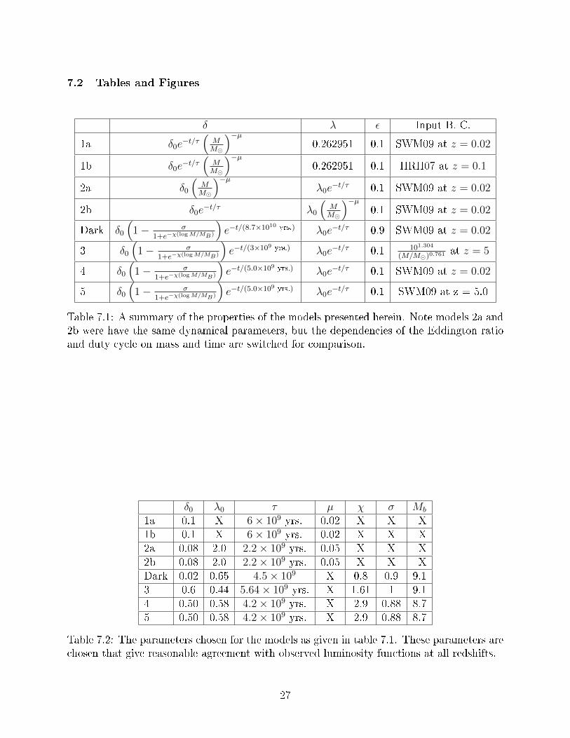
A summary of the properties of the models that were developed can be found in Tables

7.1 and 7.2. The models are numbered, and listed in the table, in the order in which they

were developed. The parameters constrained by each model inform the models that follow.

4.1 Constant Eddington Ratio

A distribution of calculated Eddington ratios is shown in Figure 7.2. This is taken from

the quasar properties catalog compiled by Shen et al. [21]. A peak for this sample from

a best-t PDF gives λ = 0.18466. It should be mentioned that this is not a ux-limited

sample. There are implications to be considered here. A ux-limited sample would possibly

be much more complete in the sense that it could be described as being representative of

the entirety of the population. However, any ux limited sample would have a cut-o with

respect to redshift and a cut-o with respect to luminosity. Since the Eddington ratio is

likely a function of redshift, as considered by McLure & Dunlop [13] and Cao [2], this could

potentially bias the sample to lower Eddington ratios. Any cut-o with respect to luminosity

13

could bias the sample to higher Eddington ratios. This analysis of Eddington ratios is not

intended to be complete; it is only an attempt to constrain the value for xed Eddington

ratio models. For this model I have adopted the mean of this distribution, λ = 0.263.

The functional form for δ(M, t) is δ0e−t/τ

(MM

)−µand the values which give the most

reasonable t to the observed luminosity functions are, δ0 = 0.1, τ = 6× 109 yrs., and µ =

0.02. In solving this equation, I have taken the solar luminosity to be L = 3.846× 1026 W,

the solar mass to be M = 1.99× 1030 kg.

A comparison of these results at dierent redshifts shows that while there is some agree-

ment, there is a great deal of room for renement. The luminosity function determined by

this method is shown in Fig. 7.3. For comparison, the luminosity function determined by

HRH07 is shown. It can be seen that there is signicant disagreement at redshifts of 0.1 and

2.0. A plot of the mass functions at various redshifts for this model is shown in Fig. 7.4. This

model has assumed a constant Eddington ratio; subsequent models will explore a variable

Eddington ratio. This initial model gives a qualitative feel for the time evolution of these

two functions (Fig. 7.5).

14

If instead, a local luminosity function is used as input and the same dynamics are applied,

the results disagree at higher redshifts. Here the solutions are for Eq. 2.9 instead of Eq. 2.8.

The results are shown in Figs. 7.6. The input luminosity function is the best-t QLF at

z = 0.1 from HRH07:

Φ(L, 0.1) =10−5.45(

L1011.94L

)0.868

+(

L1011.94L

)1.97 .

4.2 Density vs. Luminosity Evolution

In order to shed some light on the eect of mass and time dependencies on the accretion rate

parameters, I present two models which contrast these eects. In one model, the Eddington

ratio depends on time and the duty cycle depends on mass. The other model supposes an

Eddington ratio that decays with mass and a duty cycle decays that with time. I have

modeled these with identical parameters so the the evolution of the mass functions is the

same, however the dierence between the luminosity functions is signicant. The results

are shown in Figures 7.8 and 7.9. It can be seen by comparing the luminosity functions

for these that a time-dependent Eddington ratio contributes to luminosity evolution and a

time-dependent duty cycle contributes to the density evolution. This is most evident in the

luminosity function for the spiral AGN (Fig. 7.9).

4.3 Dark Accretion

This section considers an alternative model to those presented previously. The basis for this

model is the idea that tidal disruption of in-falling stellar material is responsible for the

15

bulk of the luminosity of AGN. The implications of this idea are explored, and ultimately it

is found that this is not a viable alternative to the widely accepted model of the accretion

engine.

4.3.1 Diminished eciency

Suppose that the primary mechanism for the AGN fueling is from tidal forces acting on the

in-falling matter. The primary region in which this tidal disruption would occur would be

within the Roche limit. As the black hole accretes matter, the event horizon would grow

and eventually exceed the Roche limit. For a non-rotating black hole with stellar density

material, this would be around logM/M = 8.7. Perhaps the most straightforward way to

represent this in terms of the accretion dynamics would be with an eciency parameter that

decreases at the break mass,

ε = ε0

(1− σ

1 + e−χ(logM/MB)

)(4.1)

where ε0 is the maximum eciency, σ is the fractional contribution of tidal forces to the

accretion engine, and χ controls the transition at the break.

There are two important implications of this: since the eciency parameter decreases,

so then does the luminosity. The accretion then proceeds `dark'. The other implication is

that the accretion onto the black hole actually increases as a result, since matter/energy is

no longer radiated out.

Additionally, it should be considered that the Eddington ratio is not a free parameter.

Consider a black hole with matter in-falling at some fueling rate Mf . This fueling rate is

16

not dependent on the activity within the accretion disk (ignoring feedback). This is related

to the accretion rate by

Mf =M

(1− ε)(4.2)

so the Eddington ratio becomes

λ =εMf tEM

. (4.3)

The Eddington ratio must then be a function of the eciency parameter, which is itself

likely a function of mass. Now since the luminosity function can be found from the mass

function by

Φ(L, t) = N(M, t)M=LtE/λc2

and the Eddington ratio is a function of mass, this leads to a transcendental equation for

the chosen form for ε and for fueling rates that are mass-dependent. Solutions may be found

for the mass function, but not for the luminosity function.

4.3.2 Accretion without radiation

Another approach which avoids this problem is to incorporate the tidal disruption into the

duty cycle. The duty cycle was dened as the probability that a particular black hole

would be accreting at a given time. If we modify this interpretation in consideration of this

`dark' accretion model, it could be thought of as the probability that a black hole would be

luminous at a given time, however it may still be accreting. Modeling the duty cycle in the

17

same manner as the eciency parameter:

δ = δ0

(1− σ

1 + e−χ(logM/MB)

)(4.4)

This can be implemented by solving Eq. 2.8 with a slight modication:

−2H0

3(1 + z)5/2∂N

∂z+λ(1− ε)εtE ln 10

∂N

∂ logM/M= S(M, z) (4.5)

Notice that the duty cycle does not appear in the accretion coecient this time. The

luminosity function can then be extracted in the same manner as before: from Eq. 2.10. The

chosen form for the Eddington ratio for this model is λ = λ0e−t/τ and the duty cycle has the

form given in Eq. 4.4 with an exponential time-dependency as well.

The result of this is that mass is accreted much faster. Since accretion is not limited by

the duty cycle, the resulting mass and luminosity functions are not consistent with observed

mass and luminosity functions. This model can be matched to observations by adopting an

eciency parameter ε = 0.9, which is physically unrealistic. The results of this model are

shown in Figs. 7.10 and 7.11. It would seem then that the contribution of tidally disruptive

`dark' accretion is negligible.

4.4 Break in Duty Cycle

Next I will take a look at a model that uses the duty cycle developed in the previous section.

The duty cycle there is relatively at, then breaks at some mass, dropping to nearly zero. In

this model, the results of which are shown in Figs. 7.12 and 7.13, I have used an input mass

18

function that is a single power law at redshift z = 5. Of note is the fact that the break in the

duty cycle here is responsible for introducing a break in the mass function and luminosity

functions. It is possible that the break in observed luminosity functions is caused by this

break in the duty cycle which is itself possibly caused by feedback [22].

Taking the same dynamics from Model 3 and using an input local mass function, the

evolved luminosity function can be tted closely to the observed luminosity function as shown

in Fig. 7.18. The evolved mass function for this model is shown in Fig. 7.19. This model

seems to be the most reasonable in terms of matching the observed mass and luminosity

functions.

19

5 Discretized Modeling

The models discussed up to now have been developed using the continuity equation.

This essentially represents the populations as continuous functions and is computationally

expedient for modeling a large number of objects. This chapter is devoted to the discus-

sion of a model where the objects are modeled individually and evolved through time in a

probabilistic manner dictated by the duty cycle.

5.1 Algorithm

The population is established with pseudorandom masses distributed according to the mass

function from SWM09 at z = 5. The masses then evolve iteratively through time, where at

each iteration the probability of accretion is determined by the duty cycle. When accretion

occurs, it is determined by M∆t where ∆t is the time step for the iteration. At the end of

a redshift interval, the luminosity function is calculated from the black holes that accreted

at the last iteration. This is then repeated for each redshift interval.

5.2 Implications

This has two advantages over the previous method. First, it requires no articial boundary

conditions. Second, it is relatively straightforward to introduce the eect of mergers without

propagating the entire population to lower number densities. For comparison, the results of

this model are presented with no mergers (5a), `dark' mergers (5b), and mergers that result in

an increase in luminosity (5c). The modeling of mergers in this fashion is somewhat primitive.

For this model I chose the probability of a merger per Gyr. to be 0.4 for an individual black

20

hole. This probability is somewhat exaggerated simply to illustrate the qualitative eect

of mergers. For Model 5c, where the mergers produce an increase in luminosity, this was

implemented by introducing an eciency parameter η that represents the fraction of the

merging body mass that contributes to the luminosity during the merger. For this case I

chose η = 0.2. This model is not intended to be comprehensive, and it requires further study.

This model is introduced and the results are presented to illustrate the eect of mergers.

The luminosity and mass functions of these models are shown in Figs. 7.20 - 7.25.

It should be pointed out that the parameters for accretion in Model 5 dier from those

in Model 4. Each was chosen to provide a best t to the observed luminosity function. They

dier because they rely on dierent input mass functions: Model 4 has the MF from SWM09

at z = 0.02 and Model 5 has a single power law tted to the mass function from SWM09 at

z = 5. Model 4 ts the observed luminosity functions fairly well; Model 5a ts the observed

luminosity functions at higher luminosities, and ts the mass functions from SWM09 as well.

One consequence of this approach is that it forces special attention to be paid to the low

mass end of the function. With this approach, the bulk of the objects are in that regime, so

the shape of the function becomes important at the low mass/luminosity end. These objects

contribute greatly to the evolution of the mass/luminosity function. However, this presents

diculties in implementation since computation time depends directly on the number of

objects modeled. To balance this, I have restricted the objects to logM/M > 2. The

total number of objects used in the starting sample was 1,040,921, and it was run with 10

iterations per unit redshift.

21

6 Conclusion

The results presented herein indicate that any model based on a tidal disruption of in-

falling material is untenable given the dynamics assumed here. Additionally the agreement

between observed and derived mass and luminosity functions for models with a duty cycle

with a break with mass seem to indicate that there is some mechanism responsible for the

break, and it is most likely a result of feedback. Discretized models seem to indicate that

mergers cause a mass evolution, as expected, and any model incorporating mergers may

imply a lower Eddington ratio to match observed luminosity functions (though this was not

explored in this research).

6.1 Spiral AGN functions

Much of the discussion up to this point has dealt with the comparison between the complete

luminosity functions and the luminosity functions derived in the models developed herein.

It would be useful at this point to discuss the spiral galaxy mass and luminosity functions.

First, the evolution of the spiral AGN luminosity function provides a constraint on the

dynamics in general. Any dynamics that allow a luminosity function for spiral AGN to

exceed that of the AGN population as a whole are not viable and so set constraints on

allowed dynamics.

Another point worth mentioning, as pointed out in Section 4.2, the peak of the spiral

AGN luminosity function can be used to surmise density evolution or luminosity evolution.

The propagation of the peak in the spiral AGN function is more obvious than the propagation

of the break in a double power law luminosity function. It should be pointed out however,

22

that the peak may be articial. It is likely that the low mass end of the spiral SMBH mass

function is underestimated [5]. It is possible that with more estimates of the low mass end

of this function, it may turn out to have a double power law shape. It should be mentioned

again that the dynamics applied to the spiral AGN in this research are the same dynamics

applied to the complete AGN population This work assumes that the dynamics that govern

black holes in spiral galaxies are the same as those found in early-type galaxies.

23

Bibliography

[1] Ade, P. A. R., et al. Planck 2013 results. XVI. Cosmological parameters. Astronomy &Astrophysics 571 (2014): A16.

[2] Cao, Xinwu. Cosmological evolution of massive black holes: Eects of Eddington ratiodistribution and quasar lifetime. The Astrophysical Journal 725.1 (2010): 388.

[3] Cavaliere, A., P. Morrison, and K. Wood. On Quasar Evolution. The AstrophysicalJournal 170 (1971): 223.

[4] Cavaliere, A., et al. Quasar evolution and Gravitational Collapse. The AstrophysicalJournal 269 (1983): 57-72.

[5] Davis, Benjamin L., et al. The black hole mass function derived from local spiral galax-ies. arXiv preprint arXiv:1405.5876 (2014).

[6] Ferrarese, Laura, and David Merritt. A fundamental relation between supermassive blackholes and their host galaxies. The Astrophysical Journal Letters 539.1 (2000): L9.

[7] Gebhardt, Karl, et al. A relationship between nuclear black hole mass and galaxy velocitydispersion. The Astrophysical Journal Letters 539.1 (2000): L13.

[8] Häring, Nadine. On the black hole mass-bulge mass relation. The Astrophysical JournalLetters 604.2 (2004): L89.

[9] Hartle, James B. Gravity: An Introduction to Einstein's General Relativity. San: Fran-cisco: Addison Wesley, 2003. Print.

[10] Hopkins, Philip F., Gordon T. Richards, and Lars Hernquist. An observational deter-mination of the bolometric quasar luminosity function. The Astrophysical Journal 654.2(2007): 731.

[11] Kollmeier, Juna A., et al. Black hole masses and Eddington ratios at 0.3 < z < 4. TheAstrophysical Journal 648.1 (2006): 128.

[12] Macdonald, Alan. Comment on The Cosmic Time in Terms of the Redshift, byCarmeli et al. arXiv preprint gr-qc/0606038 (2008).

[13] McLure, Ross J., and James S. Dunlop. The cosmological evolution of quasar black holemasses. Monthly Notices of the Royal Astronomical Society 352.4 (2004): 1390-1404.

[14] Peterson, Bradley M. An Introduction to Active Galactic Nuclei. Cambridge: CambridgeUniversity Press, 1997. Print.

[15] Salpeter, E. E. Accretion of interstellar matter by massive objects. The AstrophysicalJournal 140 (1964): 796-800.

[16] Schmidt, Maarten. 3C 273: a star-like object with large red-shift. Nature 197.4872(1963): 1040.

24

[17] Schmidt, Maarten. Space distribution and luminosity functions of quasi-stellar radiosources. The Astrophysical Journal 151 (1968): 393.

[18] Shankar, Francesco, David H. Weinberg, and Jordi Miralda-Escudé. Self-consistentmodels of the AGN and black hole populations: duty cycles, accretion rates, and themean radiative eciency. The Astrophysical Journal 690.1 (2009): 20.

[19] Shankar, Francesco, David H. Weinberg, and Jordi Miralda-Escudé. Accretion-drivenevolution of black holes: Eddington ratios, duty cycles, and active galaxy fractions. Monthly Notices of the Royal Astronomical Society (2012).

[20] Shapiro, Stuart L. Spin, accretion, and the cosmological growth of supermassive blackholes. The Astrophysical Journal 620.1 (2005): 59.

[21] Shen, Yue, et al. A catalog of quasar properties from Sloan Digital Sky Survey release7. The Astrophysical Journal Supplement Series 194.2 (2011): 45.

[22] Silk, Joseph, and Martin J. Rees. Quasars and galaxy formation. arXiv preprint astro-ph/9801013 (1998).

[23] Small, Todd A., and Roger D. Blandford. Quasar evolution and the growth of blackholes. Monthly Notices of the Royal Astronomical Society 259.4 (1992): 725-737.

25

7 Appendix

7.1 Cosmology

Figure 7.1: Comparison between redshift-time relation from Eq. 7.1 [12] shown as solid lineand approximation used in Eq. 2.7 (dashed line).

Here the time as a function of redshift is taken to be

t(z) =2H−1

0

3Ω1/2Λ

sinh−1

[(ΩΛ

ΩM

)1/2

(z + 1)−3/2

]. (7.1)

This approximation is valid over the range of redshifts used in this research, and is used

as a means of simplifying the forms of dierential equations being solved numerically.

26

7.2 Tables and Figures

δ λ ε Input B. C.

1a δ0e−t/τ

(MM

)−µ0.262951 0.1 SWM09 at z = 0.02

1b δ0e−t/τ

(MM

)−µ0.262951 0.1 HRH07 at z = 0.1

2a δ0

(MM

)−µλ0e

−t/τ 0.1 SWM09 at z = 0.02

2b δ0e−t/τ λ0

(MM

)−µ0.1 SWM09 at z = 0.02

Dark δ0

(1− σ

1+e−χ(logM/MB)

)e−t/(8.7×1010 yrs.) λ0e

−t/τ 0.9 SWM09 at z = 0.02

3 δ0

(1− σ

1+e−χ(logM/MB)

)e−t/(3×109 yrs.) λ0e

−t/τ 0.1 101.304

(M/M)0.761at z = 5

4 δ0

(1− σ

1+e−χ(logM/MB)

)e−t/(5.0×109 yrs.) λ0e

−t/τ 0.1 SWM09 at z = 0.02

5 δ0

(1− σ

1+e−χ(logM/MB)

)e−t/(5.0×109 yrs.) λ0e

−t/τ 0.1 SWM09 at z = 5.0

Table 7.1: A summary of the properties of the models presented herein. Note models 2a and2b were have the same dynamical parameters, but the dependencies of the Eddington ratioand duty cycle on mass and time are switched for comparison.

δ0 λ0 τ µ χ σ Mb

1a 0.1 X 6× 109 yrs. 0.02 X X X1b 0.1 X 6× 109 yrs. 0.02 X X X2a 0.08 2.0 2.2× 109 yrs. 0.05 X X X2b 0.08 2.0 2.2× 109 yrs. 0.05 X X XDark 0.02 0.65 4.5× 109 X 0.8 0.9 9.13 0.6 0.44 5.64× 109 yrs. X 1.61 1 9.14 0.50 0.58 4.2× 109 yrs. X 2.9 0.88 8.75 0.50 0.58 4.2× 109 yrs. X 2.9 0.88 8.7

Table 7.2: The parameters chosen for the models as given in table 7.1. These parameters arechosen that give reasonable agreement with observed luminosity functions at all redshifts.

27

Figure 7.2: Logarithmic distribution of the Eddington ratio for a sample of quasars. Thepeak is at λ = 0.18466. The mean value of this sample is λ = 0.262951.

Figure 7.3: The luminosity function for Model 1a at various redshifts shown in blue. Thespiral AGN luminosity function is shown in red. For comparison the observed luminos-ity function from HRH07 is plotted as blue dots. This is taken from the complete set ofobservations.

28

Figure 7.4: The mass functions for Model 1a at various redshifts shown in blue. The spiralAGN mass function is in red. The dots are calculated mass functions at the correspondingredshifts from SWM09.

Figure 7.5: The luminosity function for Model 1a at various redshifts (blue curves fromFig. 7.3 shown here on single plot). This model exhibits both luminosity and density evolu-tion as evidenced by the movement of the break.

29

Figure 7.6: The luminosity function for Model 1b at various redshifts shown in blue. Thespiral AGN luminosity function is shown in red. The observed luminosity function fromHRH07 is shown for comparison.

Figure 7.7: The mass functions for Model 1b at various redshifts shown in blue. The spiralAGN mass function is in red. The dots are calculated mass functions at the correspondingredshifts from SWM09.

30

Figure 7.8: Comparison of luminosity functions for Models 2a (top) and 2b (bottom). Bluelines are the total luminosity functions for this model. Red lines are the spiral AGN lu-minosity functions. Blue dots indicate the luminosity functions taken from HRH07. Themass functions are not shown here since they are identical for both models. The luminosityfunctions are the same for redshifts 2 < z < 5, however, they begin to show disagreement atz < 2.

31

Figure 7.9: The spiral AGN luminosity function for Models 2a and 2b. Purple denotesredshift 0.1, blue: redshift 1, green: redshift 2, orange: redshift 3, yellow: redshift 4, red:redshift 5. Notice that model 2a on the left exhibits purely luminosity evolution, as wouldbe expected with a time-varying Eddington ratio. Model 2b on the right exhibits mostlydensity evolution, as would be expected with a time-varying duty cycle.

Figure 7.10: Luminosity function of the `dark accretion' model at various redshifts. Theblue line is the LF for the entire AGN population, the red line is the spiral AGN LF. Shownfor comparison (blue dots) is the observed LF from HRH07. The results shown here dependon an eciency parameter ε = 0.9. Such a high eciency parameter renders this modelphysically unrealistic.

32

Figure 7.11: Mass function of the `dark accretion' model for spiral galaxy SMBH (red) andthe total BHMF (blue). Shown with the calculated mass functions from SWM09 (blue dots).

Figure 7.12: The luminosity function for Model 3 (blue line) with a single power law inputmass function at z = 5. The red line is the spiral AGN LF. Blue dots are the observed LFfrom HRH07 using the complete set of observations. The break in the duty cycle inducesa break in the luminosity function here giving it a double power law line-shape at lowerredshifts.

33

Figure 7.13: Mass function for Model 3, with single power law input mass function at z = 5.The input mass function is that shown in the bottom right frame. Notice that as the massfunction evolves with time, a break is introduced around logM/M ∼ 9. This is caused bythe break in the duty cycle around the same mass.

Figure 7.14: Complete mass function for Model 4 plotted as a function of mass and redshift.The time evolution of the break in the mass function can be seen qualitatively here.

34

Figure 7.15: Complete bolometric luminosity function for Model 4 as a function of redshift.

35

Figure 7.16: Mass function for spiral galaxies for Model 4.

Figure 7.17: Luminosity function for spiral AGN for Model 4.

36

Figure 7.18: Complete luminosity function (blue) and the spiral AGN luminosity function(red) computed from Model 4 plotted at various redshifts.

Figure 7.19: Complete mass function and spiral galaxy black hole mass function from Model4 shown at various redshifts. Red line is the spiral BHMF, blue line is the total BHMF. Bluedots are BHMF estimates from SWM09.

37

Figure 7.20: Luminosity function of Model 5a shown at various redshifts in red. Comparisonwith HRH07 shown in blue. Axes are not scaled the same for each plot.

Figure 7.21: Mass function of Model 5a shown at various redshifts in red and calculatedmass function from SWM09 shown in blue. Axes are not scaled the same for each plot.

38

Figure 7.22: Luminosity function of Model 5b (red) including the eect of mergers on pop-ulation. Comparison with HRH07 shown in blue. Axes are not scaled the same for eachplot.

Figure 7.23: Mass function of Model 5b (red) including the eect of mergers on populationshown with mass functions from SWM09 in blue. Axes are not scaled the same for each plot.

39

Figure 7.24: Luminosity function of Model 5c (red) including the eect of mergers on pop-ulation and luminosity. Comparison with HRH07 shown in blue. Axes are not scaled thesame for each plot.

Figure 7.25: Mass function of Model 5c (red) including the eect of mergers on populationand luminosity. Comparison with SWM09 shown in blue. This mass function is almostidentical to that of Model 5b. There are slight variations at the high mass end due tosmaller sample sizes in that regime and the stochastic nature of the accretion and mergers.Axes are not scaled the same for each plot.

40