population sample parameter: proportion p count mean median statistic: proportion count mean median
TRANSCRIPT
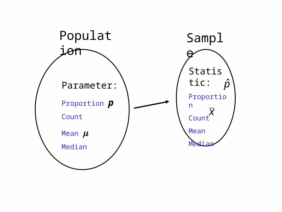
Population Sample
Parameter:
Proportion p
Count
Mean Median
Statistic:
Proportion
Count
Mean
Median
x
p̂
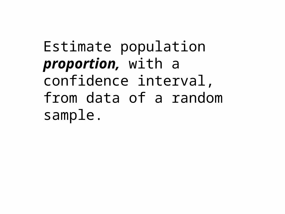
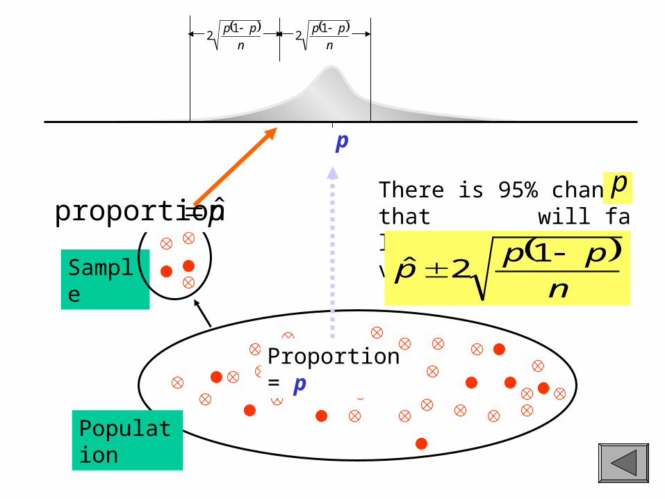
Estimate population proportion, with a confidence interval, from data of a random sample.
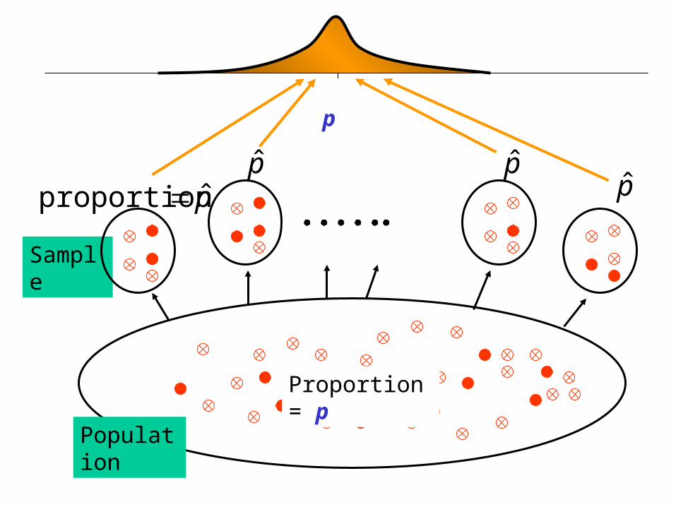
Population
Proportion = p
Sample
p̂proportion
p
p̂ p̂p̂
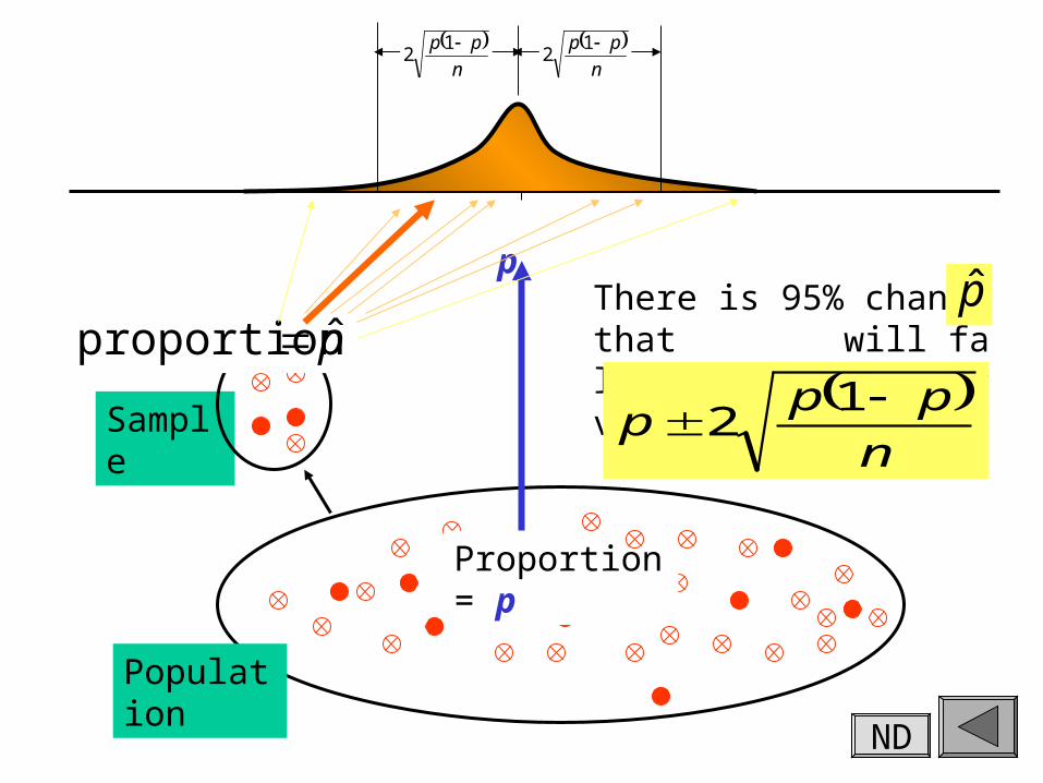
Population
Proportion = p
Sample
p̂proportion
p
There is 95% chance that will fall inside the interval
p̂
n
ppp
12
n
pp 12
n
pp 12
ND
Population
Sample
p̂proportion
Proportion = p
p
There is 95% chance that will fall inside the interval
n
ppp
12ˆ
p
n
pp 12
n
pp 12

Population
Sample
p̂proportion
Proportion = p
p
There is 95% chance that will fall inside the interval
n
ppp
ˆ1ˆ2ˆ
p
n
pp ˆ1ˆ2
n
pp ˆ1ˆ2
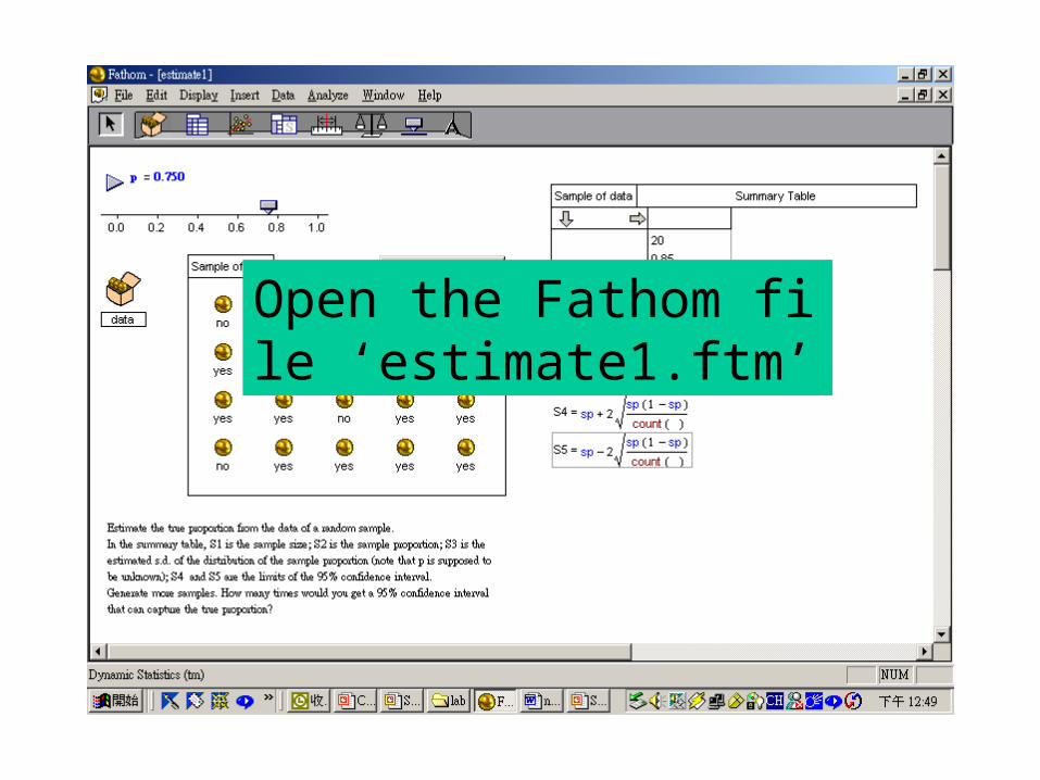
Open the Fathom file ‘estimate1.ftm’
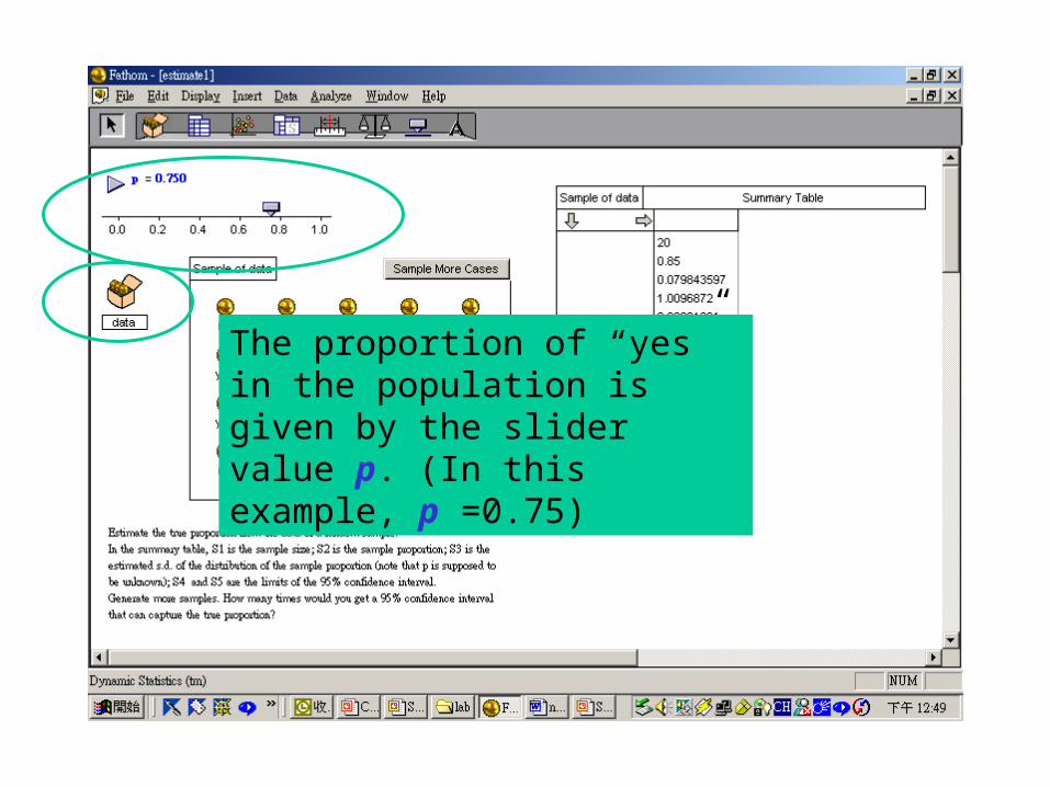
The proportion of “yes” in the population is given by the slider value p. (In this example, p =0.75)
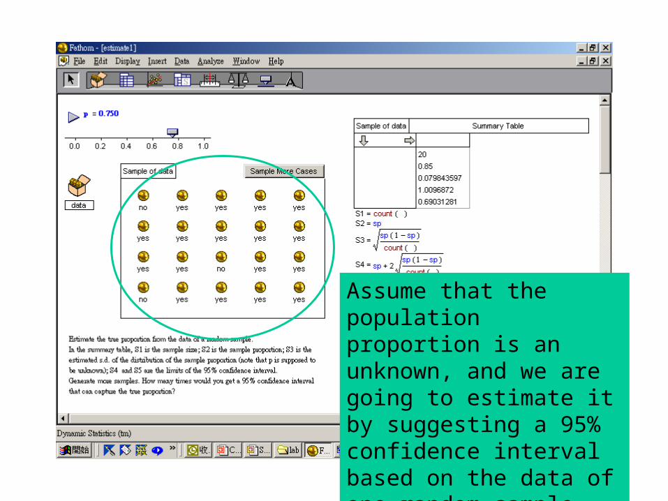
Assume that the population proportion is an unknown, and we are going to estimate it by suggesting a 95% confidence interval based on the data of one random sample.
Size of this sample is n = 20.
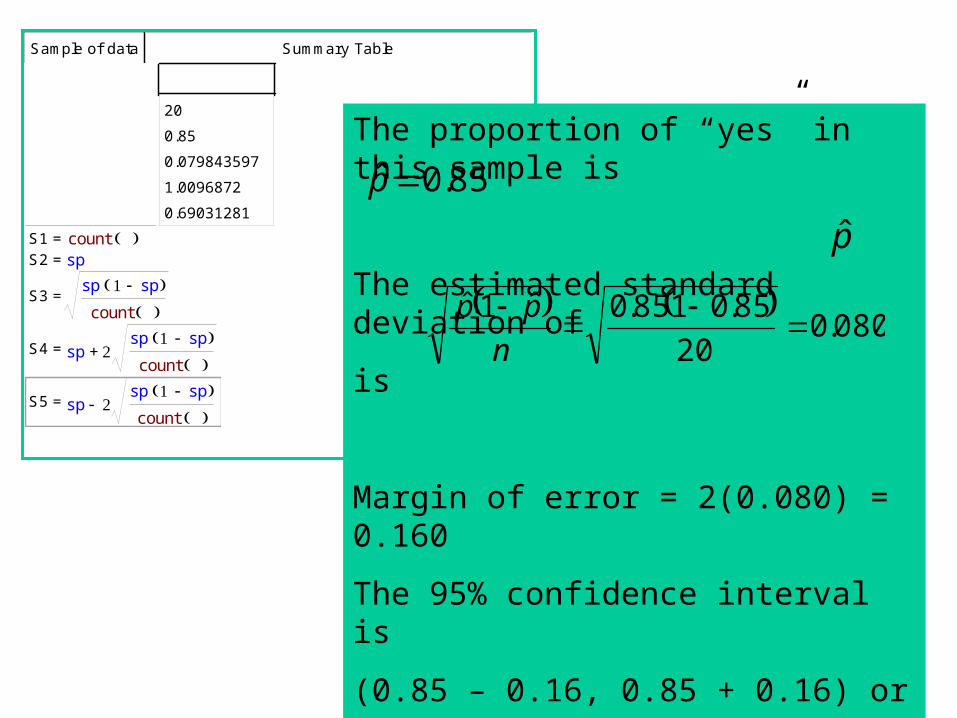
Summary TableSample of data
20
0.85
0.079843597
1.0096872
0.69031281
S1 = countS2 = sp
S3 = sp sp
count
S4 = sp sp sp
count+
S5 = sp sp sp
count
The proportion of “yes” in this sample is
The estimated standard deviation of
is
Margin of error = 2(0.080) = 0.160
The 95% confidence interval is
(0.85 – 0.16, 0.85 + 0.16) or
(0.69, 1.01)
85.0ˆ p
p̂
080.0
20
85.0185.0ˆ1ˆ
n
pp
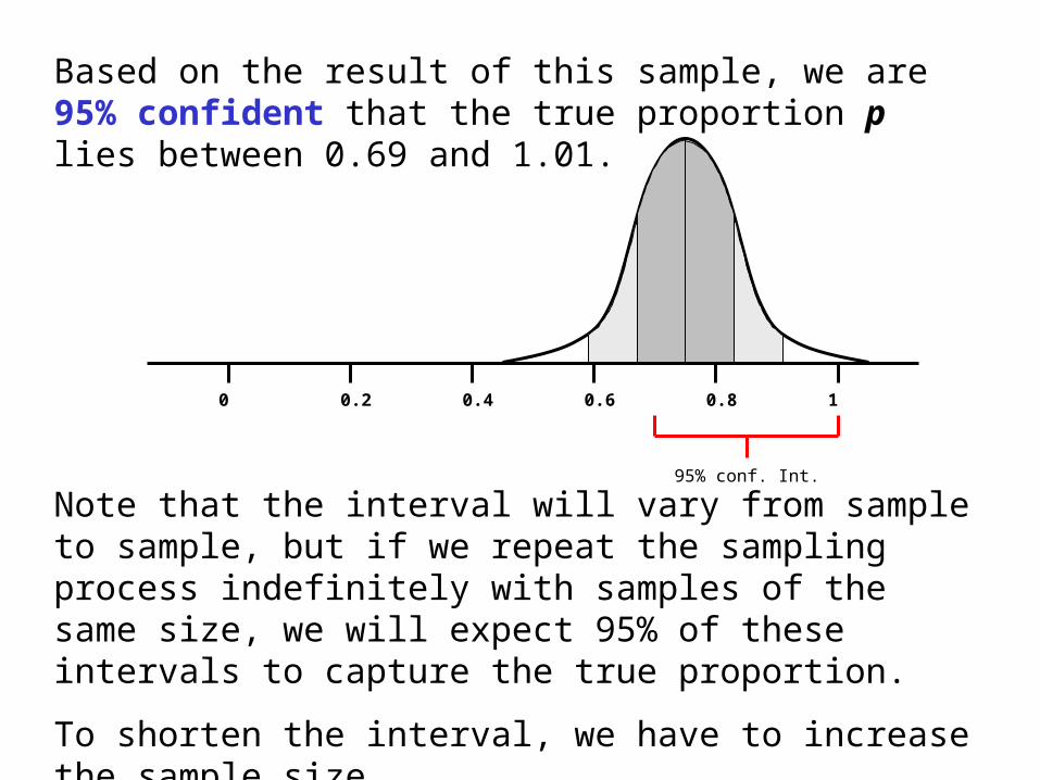
Based on the result of this sample, we are 95% confident that the true proportion p lies between 0.69 and 1.01.
Note that the interval will vary from sample to sample, but if we repeat the sampling process indefinitely with samples of the same size, we will expect 95% of these intervals to capture the true proportion.
To shorten the interval, we have to increase the sample size.
0 0.2 0.4 0.6 0.8 1
95% conf. Int.
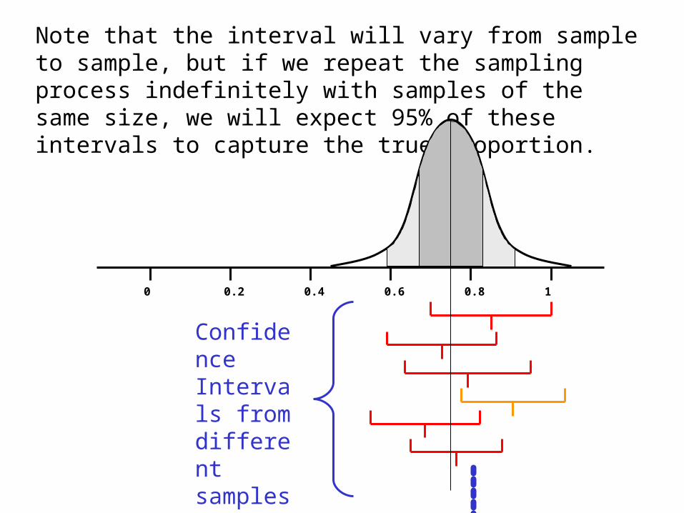
Note that the interval will vary from sample to sample, but if we repeat the sampling process indefinitely with samples of the same size, we will expect 95% of these intervals to capture the true proportion.
0 0.2 0.4 0.6 0.8 1
Confidence Intervals from different samples
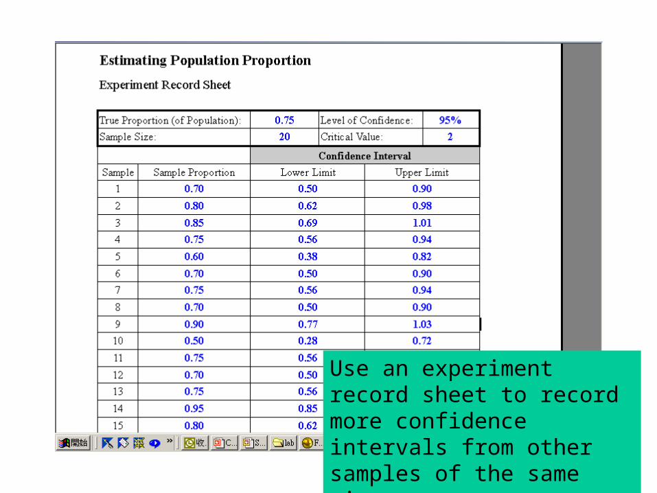
Use an experiment record sheet to record more confidence intervals from other samples of the same size.
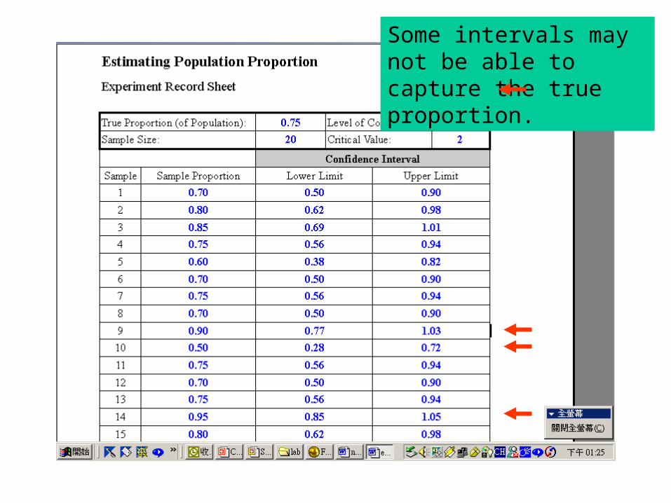
Some intervals may not be able to capture the true proportion.
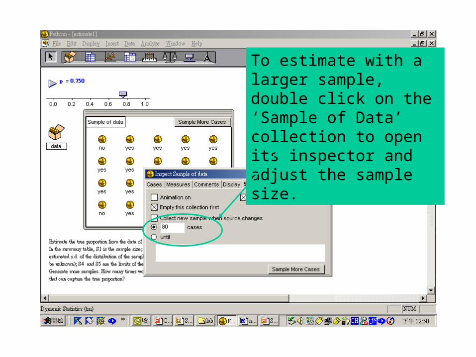
To estimate with a larger sample, double click on the ‘Sample of Data’ collection to open its inspector and adjust the sample size.
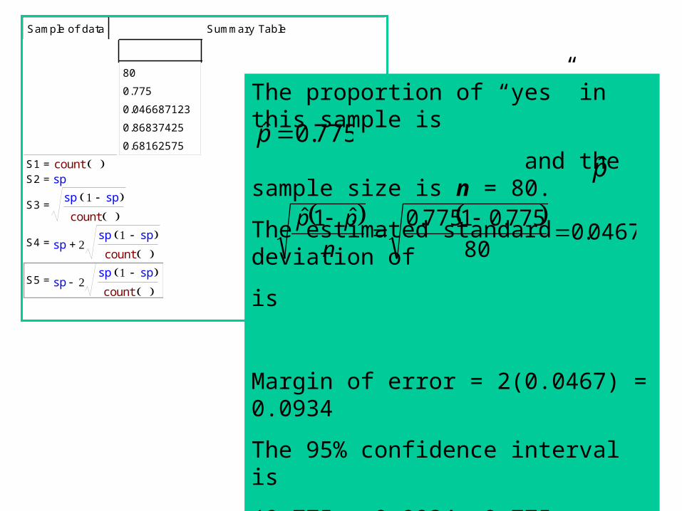
Summary TableSample of data
80
0.775
0.046687123
0.86837425
0.68162575
S1 = countS2 = sp
S3 = sp sp
count
S4 = sp sp sp
count+
S5 = sp sp sp
count
The proportion of “yes” in this sample is
and the sample size is n = 80.
The estimated standard deviation of
is
Margin of error = 2(0.0467) = 0.0934
The 95% confidence interval is
(0.775 – 0.0934, 0.775 + 0.0934) or
(0.682, 0.868)
775.0ˆ pp̂
0467.0
80
775.01775.0ˆ1ˆ
n
pp
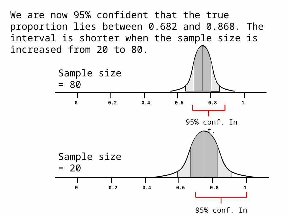
0 0.2 0.4 0.6 0.8 1
95% conf. Int.
Sample size = 20
0 0.2 0.4 0.6 0.8 1
95% conf. Int.
Sample size = 80
We are now 95% confident that the true proportion lies between 0.682 and 0.868. The interval is shorter when the sample size is increased from 20 to 80.
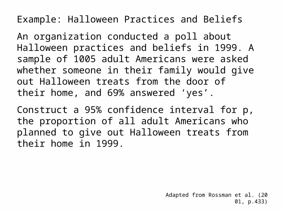
Example: Halloween Practices and Beliefs
An organization conducted a poll about Halloween practices and beliefs in 1999. A sample of 1005 adult Americans were asked whether someone in their family would give out Halloween treats from the door of their home, and 69% answered ‘yes’.
Construct a 95% confidence interval for p, the proportion of all adult Americans who planned to give out Halloween treats from their home in 1999.
Adapted from Rossman et al. (2001, p.433)
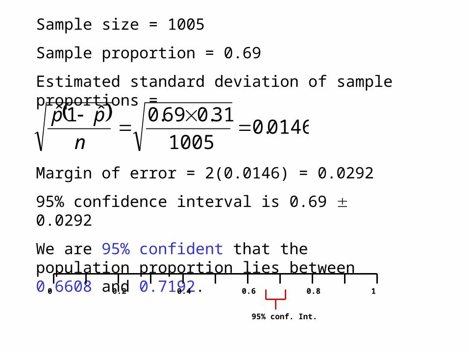
Sample size = 1005
Sample proportion = 0.69
Estimated standard deviation of sample proportions =
0146.0
1005
31.069.0ˆ1ˆ
n
pp
Margin of error = 2(0.0146) = 0.0292
95% confidence interval is 0.69 0.0292
We are 95% confident that the population proportion lies between 0.6608 and 0.7192.
0 0.2 0.4 0.6 0.8 1
95% conf. Int.
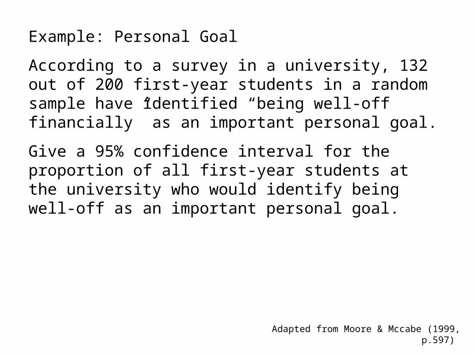
Example: Personal Goal
According to a survey in a university, 132 out of 200 first-year students in a random sample have identified “being well-off financially” as an important personal goal.
Give a 95% confidence interval for the proportion of all first-year students at the university who would identify being well-off as an important personal goal.
Adapted from Moore & Mccabe (1999, p.597)
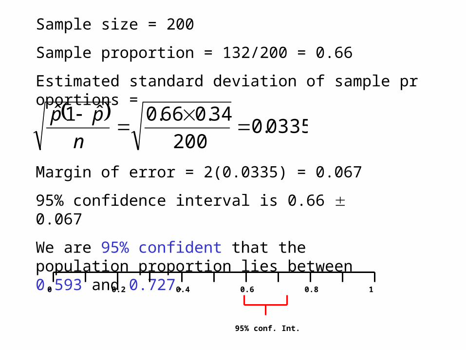
Sample size = 200
Sample proportion = 132/200 = 0.66
Estimated standard deviation of sample proportions =
0335.0
200
34.066.0ˆ1ˆ
n
pp
Margin of error = 2(0.0335) = 0.067
95% confidence interval is 0.66 0.067
We are 95% confident that the population proportion lies between 0.593 and 0.727.
0 0.2 0.4 0.6 0.8 1
95% conf. Int.
Estimate population mean, with a confidence interval, from data of a random sample.
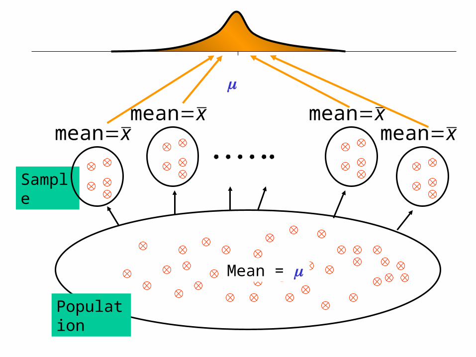
Population
Mean =
Sample
xmeanxmean
xmeanxmean
Population
Mean =
Sample
xmean
n
2
n
2
s.d. =
There is 95% chance that will fall inside the interval
x
n
2
ND
Population
Sample
xmean
Mean =
n
2
n
2
s.d. =
There is 95% chance that will fall inside the interval
nx
2
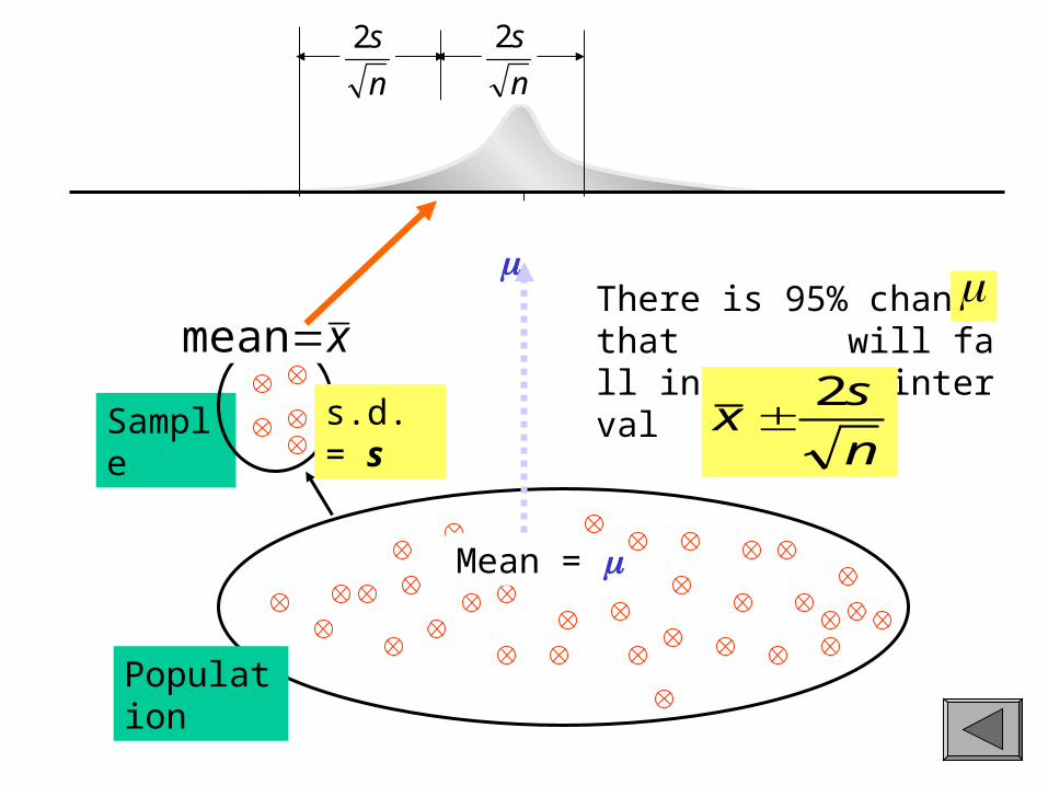
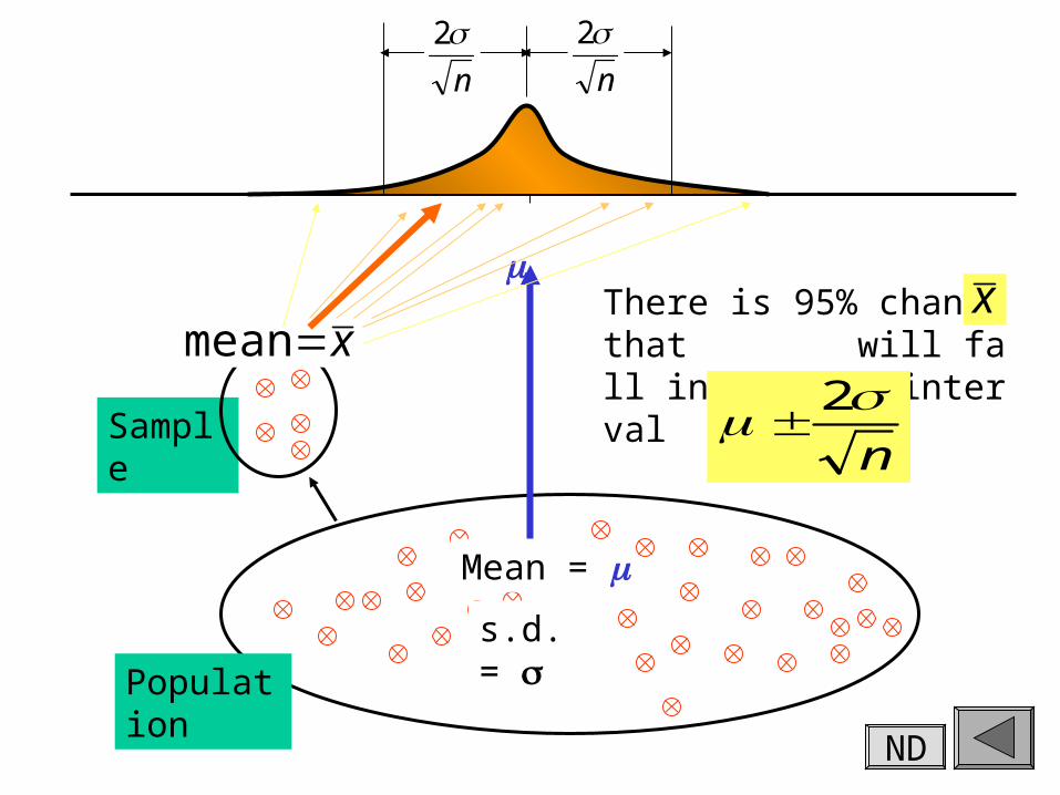
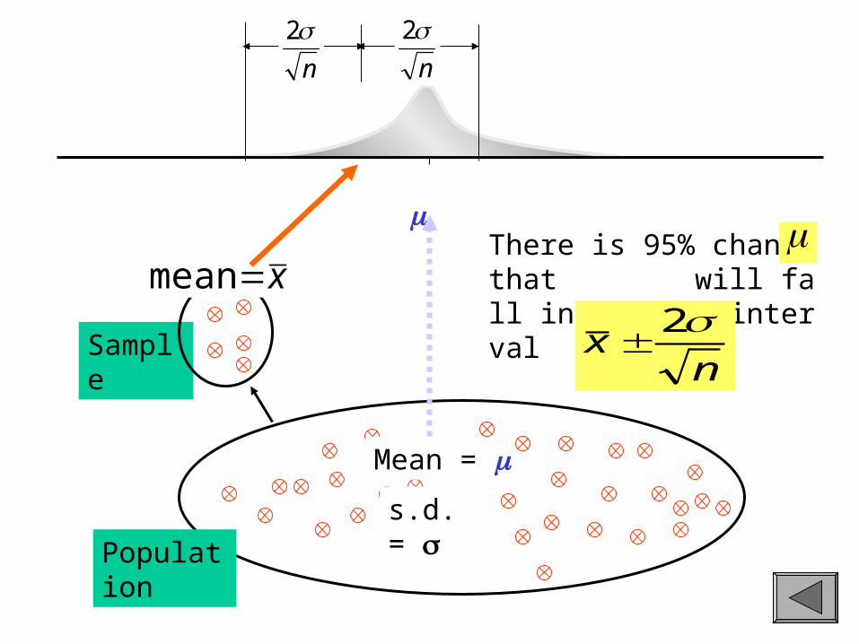
Population
Sample
xmean
Mean =
n
s2
n
s2
s.d. = s
There is 95% chance that will fall inside the interval
n
sx
2
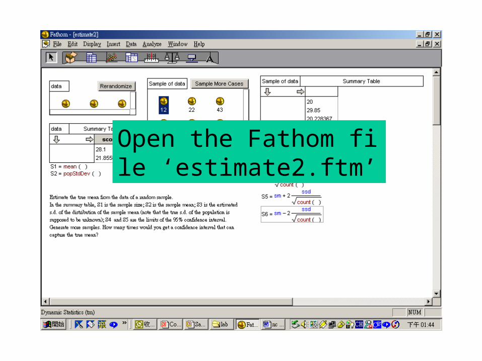
Open the Fathom file ‘estimate2.ftm’
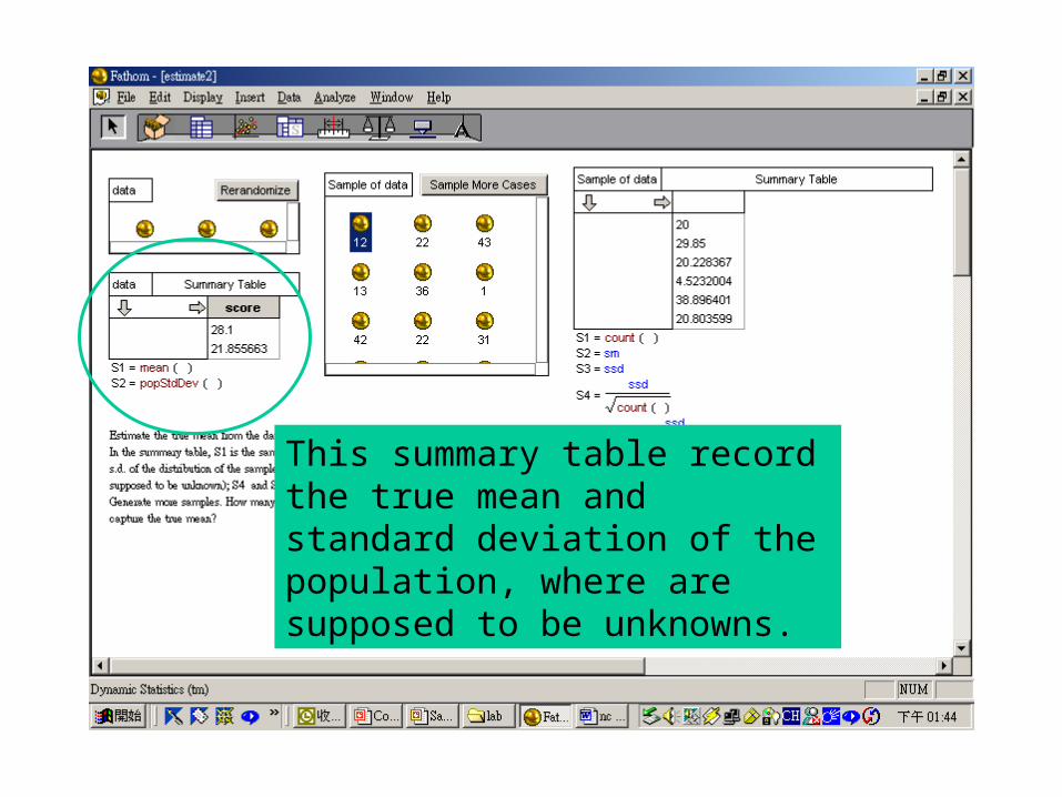
This summary table record the true mean and standard deviation of the population, where are supposed to be unknowns.
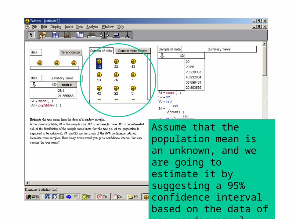
Assume that the population mean is an unknown, and we are going to estimate it by suggesting a 95% confidence interval based on the data of one random sample.
Size of this sample is n = 20.
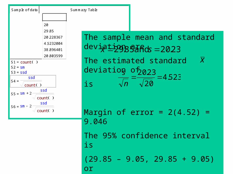
Summary TableSample of data
20
29.85
20.228367
4.5232004
38.896401
20.803599
S1 = countS2 = smS3 = ssd
S4 = ssd
count
S5 = sm ssd
count+
S6 = sm ssd
count
The sample mean and standard deviation are
The estimated standard deviation of
is
Margin of error = 2(4.52) = 9.046
The 95% confidence interval is
(29.85 – 9.05, 29.85 + 9.05) or
(20.80, 38.90)
23.20 and 85.29 sxx
523.420
23.20
n
s
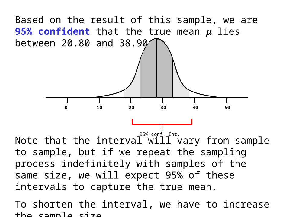
Based on the result of this sample, we are 95% confident that the true mean lies between 20.80 and 38.90.
Note that the interval will vary from sample to sample, but if we repeat the sampling process indefinitely with samples of the same size, we will expect 95% of these intervals to capture the true mean.
To shorten the interval, we have to increase the sample size.
0 10 20 30 40 50
95% conf. Int.
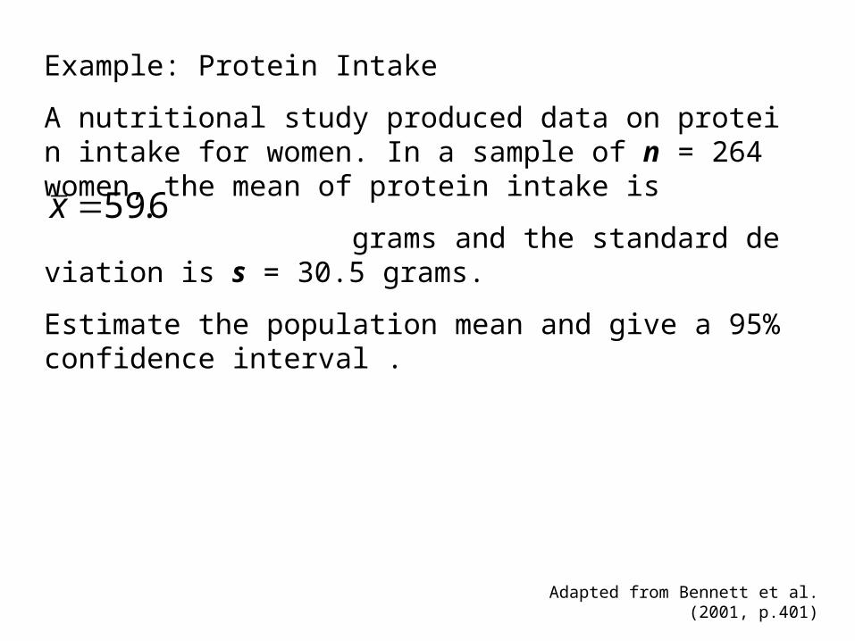
Example: Protein Intake
A nutritional study produced data on protein intake for women. In a sample of n = 264 women, the mean of protein intake is
grams and the standard deviation is s = 30.5 grams.
Estimate the population mean and give a 95% confidence interval .
6.59x
Adapted from Bennett et al. (2001, p.401)
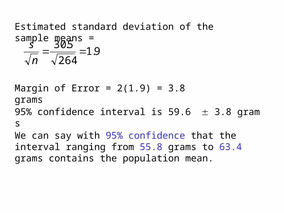
Estimated standard deviation of the sample means =
9.1264
5.30
n
s
Margin of Error = 2(1.9) = 3.8 grams
95% confidence interval is 59.6 3.8 grams
We can say with 95% confidence that the interval ranging from 55.8 grams to 63.4 grams contains the population mean.
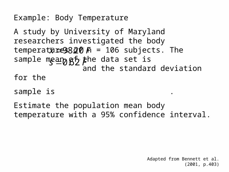
Example: Body Temperature
A study by University of Maryland researchers investigated the body temperatures of n = 106 subjects. The sample mean of the data set is and the standard deviation for the
sample is .
Estimate the population mean body temperature with a 95% confidence interval.
Fx 20.98Fs 62.0
Adapted from Bennett et al. (2001, p.403)
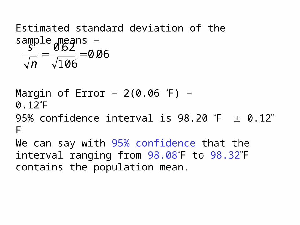
Estimated standard deviation of the sample means =
06.0106
62.0
n
s
Margin of Error = 2(0.06 F) = 0.12F
95% confidence interval is 98.20 F 0.12F
We can say with 95% confidence that the interval ranging from 98.08F to 98.32F contains the population mean.
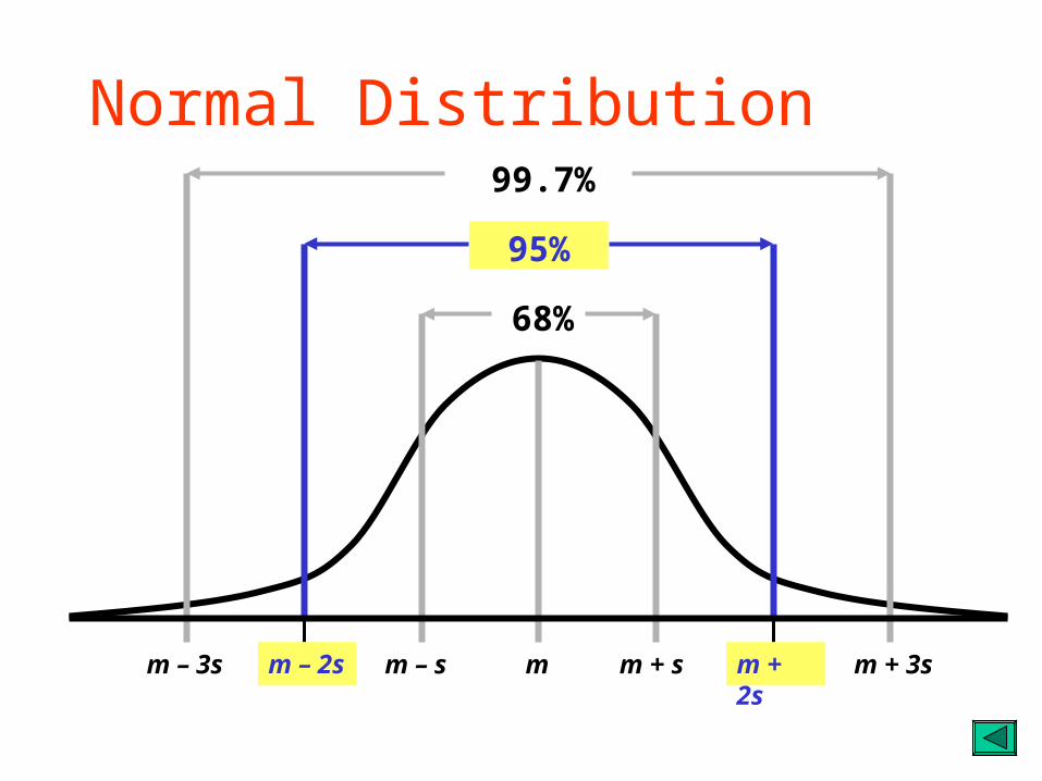
Normal Distribution
m – s mm – 2s m – 3s m + s m + 2s m + 3s
68%
95%
99.7%