population stochastic modelling (psm): model de nition
TRANSCRIPT

Population Stochastic Modelling (PSM):
Model definition, description and examples
Stig Mortensen and Søren Klim
November 5, 2018
Package: PSM, version 0.8-12URL: http://www.imm.dtu.dk/psm
Contents
1 Introduction 1
2 Model definition 2
3 Estimation 3
4 User’s guide to PSM 7
5 Examples 105.1 Dosing in two-compartment model (Linear) . . . . . . . . . . . . 115.2 Extraction of insulin secretion rate (Linear) . . . . . . . . . . . . 16
References 23
1 Introduction
Functions for fitting linear and non-linear mixed-effects models using stochasticdifferential equations (SDEs). The package allows for any multivariate non-linear time-variant model to be specified, and it also handles multidimensionalinput, covariates, missing observations, and specification of dosage regimen. Theprovided pipeline relies on the coupling of the FOCE algorithm and Kalmanfiltering as outlined by Klim et al (2009, <doi:10.1016/j.cmpb.2009.02.001>)and has been validated against the proprietary software ’NONMEM’ (Tornoeet al, 2005, <doi:10.1007/s11095-005-5269-5>). Further functions are providedfor finding smoothed estimates of model states and for simulation.
Some of the most essential parts of the implentation, namely the Kalmanfilter, is for linear models run using compiled code written in Fortran, whichgives significant improvements in the parameter estimation times in R. However,
1

otherwise this version is almost entirely created in R, and estimation times arethus in no way comparable to state-of-the-art software for similar types of modelsbased on ordinary differential equations.
2 Model definition
A mixed-effects model is used to describe data with the following general struc-ture
yij , i = 1, ..., N, j = 1, ..., ni (1)
where yij is a vector of measurements at time tij for individual i, N is thenumber of individuals and ni is the number of measurements for individual i.In a mixed-effects model the variation is split into intra-individual variation andinter-individual variation, which is modelled by a first and second stage model.For further detail regarding the model definition please refer to [1, 2, 3].
First stage model
The first stage model for a mixed effects model can be written in the form ofa state space model. A state space model consists of two parts, namely a setof continuous state equations defining the dynamics of the system and a set ofdiscrete measurement equations, which defines a functional relationship betweenthe states of the system and the obtained measurements. In the linear form thestate space equations are written as
dxt = (A(φi)xt +B(φi)ut)dt+ σω(φi)dωt (2)
yij = C(φi)xij +D(φi)uij + eij (3)
and for a general non-linear model as
dxt = f(xt,ut, t,φi)dt+ σ(ut, t, φi)dωt (4)
yij = g(xij ,uij , tij ,φi) + eij (5)
where t is the continuous time variable, the states of the model and the optionalinputs at time t are denoted xt and ut respectively and ωt is a standard Wienerprocess such that ωt2 − ωt1 ∈ N(0, |t2 − t1|I). Both the state, measurementand input can be multi-dimensional, and are in such cases thus represented by avector at time tij . The input is assumed constant between sample times (zero-order hold). The individual model parameters are denoted φi. Measurementsare assumed observed with a Gaussian white noise measurement error, thatis eij ∈ N(0,S(φi)). For a non-linear model the covariance matrix may alsodepend on input and time, that is S(ut, t,φi)).
2

In the evaluation of the non-linear model it is necessary to specify a Jacobianmatrix function with first-order partial derivatives for f and g. These functionsare defined as
∂f
∂xt,
∂g
∂xt(6)
and must be given with the model specification. PSM will check the user definedJacobian functions with numerical evaluations of the Jacobians of f and g toensure that they are correct. It is possible to avoid specifying the Jacobianfunctions in the model and use numerical approximations instead, but this willincrease estimation time at least ten-fold. See the help file in R for PSM.estimatefor details regarding this.
The initial state of the model is given as a function of t1, φi, and ui1 anddefines the model state at time t1 before update based on the first observation.The initial state can thus be included in the parameter estimation as necessary.The covariance matrix of the initial state is set to the integral of the Wienerprocess and the dynamics of the system over the first sample interval t2 − t1 asalso done in [3].
The concept of states is essential to the understanding of the model setup.The state vector describes the state of the entire system and is only observablethrough measurement noise. The actual relation between measurements andstates is defined in the measurement equation (3). A state can represent manydifferent aspects of the system of interest, e.g. concentrations or amounts incompartments, a volume, a parameter with unknown time varying behavior oran input to the system, that we wish to estimate.
Second stage model
The second stage model describes the variation of the individual parameters φi
between individuals and is defined as
φi = h(θ,ηi,Zi) (7)
where ηi is the multivariate random effect parameter for the ith individual,which is assumed Gaussian distributed with mean zero and covariance Ω, i.e.ηi ∈ N(0,Ω). The fixed effect parameter of the model is θ and Zi is a vectorof co-variates for the ith individual.
3 Estimation
Parameter estimation is done using maximum likelihood. The likelihood func-tion will only be outlined briefly here, so please refer to [1, 2, 3] for a detaileddescription.
The full set of model parameters to be estimated for the final mixed effectsmodel based on SDEs are the matrices Σ, σω, Ω and the fixed effect parametersin the vector θ. The three matrices are usually fixed to some degree so that
3

only the diagonals or other partial structure remains to be estimated. In PSMthe parameters in Σ and σω are included in θ.
In PSM the function ModelPar defines which part of the model parametersshould estimated. These parameters are denoted Θ (in PSM: THETA) such that
ModelPar : Θ→ (θ,Ω). (8)
The exact population likelihood function cannot be evaluated analyticallyand thus a second-order Taylor expansion is made of the individual a posteriorilog-likelihood function around the value of ηi that maximizes it. The objectivefunction for PSM is thereby given as
− logL(Θ) ≈N∑i=1
(1
2log
∣∣∣∣−∆li2π
∣∣∣∣− li) (9)
where li is the a posteriori log-likelihood function for the ith individual. Thislikelihood function is evaluated using the Kalman Filter which gives an exactsolution for linear models. For non-linear models the Extended Kalman filter(EKF) is used which is only an approximation. The 2nd derivative ∆li isapproximated using the First-Order Conditional Estimation (FOCE) method,in the same way as it is normally done in mixed effects models based on ordinarydifferential equations (ODEs).
Uncertainty of parameters
PSM estimates the uncertainty for the parameter estimates based on the ob-served Fisher information. The parameters to be estimated are denoted Θ andthe observed information is then defined as
j(Θ) = − ∂2
∂Θ∂ΘTlogL(Θ) = −∇2 logL(Θ) (10)
which is equal to the Hessian matrix of the negative log-likelihood function.If the parameters maximizing the likelihood function are called Θ they willasymptotically have the distribution
Θ ∼ N(Θ, j(Θ)−1). (11)
This is used in PSM to provide a Wald 95% confidence interval, standarderror and correlation matrix for the estimates. The Hessian is evaluated usinghessian in the numDeriv package.
State estimates
A key feature of the SDE approach to population modelling is the ability togive improved estimates of the system states given the individual parametersand also to provide confidence bands for the states. Confidence bands at a time
4

point t are directly given by the estimated state covariance matrix P i(t|...) fromthe EKF, where t can be both at or between measurements.
There are four types of state and state covariance estimates available whenusing the EKF, each of which differs in the way data is used. The four typesare:
• Simulation estimate: xi(j|0), P i(j|0)Provides an estimate of the state evolution for a repeated experiment,without updating based on measurements. This is an ODE-like estimate,but it also yields a confidence band for the state evolution.
• Prediction estimate: xi(j|j−1), P i(j|j−1)The prediction is used here to give the conditional density for the nextobservation at time tij given the observations up to ti(j|j−1).
• Filtering estimate: xi(j|j), P i(j|j)Best estimate at time tij given the observations up to time tij .
• Smoothing estimate: xi(j|N), P i(j|N)
Optimal estimate at time tij utilizing all observations both prior to andafter time tij .
For a conventional ODE model the state is found by the simulation estimate,which is entirely given by the (possibly ML-estimated) initial state of the system.The covariance matrix for the states is 0 since no system noise is estimated.
With SDEs three new types of estimates, apart from the simulation estimate,also become available. In the present setup the prediction estimate is used togive conditional Gaussian densities to form the likelihood function. The filterestimate is the best obtainable state estimate during the experiment, where thesubsequent observations are not present. The third type of state estimate isthe smoothed estimate. This provides the optimal state and state covarianceestimate (xi(j|N) and P i(j|N)) based on all obtained observations, both priorand subsequent to the time of interest. The smoothed estimate is thereforeoften the natural estimate of choice when studying the behavior of the systemin post hoc analysis [1].
Comparison to NONMEM
The NONMEM software is a widely used tool for mixed effects modelling basedon ODEs [4]. NONMEM also performs maximum likelihood estimation usingthe FOCE approximation and for many it might thus be of interest to knowhow the two objective functions are related.
The objective function in NONMEM (lNM ) is advertised as −2 logL but infact it lacks a constant equal to the likelihood of the data. The PSM objectivefunction (lPSM ) is − logL as seen in Eq. (9) and the relation thereby becomeslNM = 2 · lPSM − log(2π) ·
∑ni. The relation has been tested for a number of
models [1].
5

Models with no random effects
A special case arises in models where no random effects are specified. This maybe defined in PSM by setting OMEGA = NULL in the ModelPar function. Thisgreatly simplifies the likelihood function, as it is no longer necessary to integrateout the random effects. The likelihood function is thus reduced to a productof conditional probabilities of the observations. In the form of a log-likelihoodfunction this may be written as
− logL(Θ) = −N∑i=1
ni∑j=1
log p(yij |·) (12)
where the · indicates conditioning on parameters and past observations for in-dividual i. The latter conditioning is necessary due to the inclusion of SDEs inthe model.
The likelihood function in Eq. (12) is identical to the one used in CTSM[3], and is sometimes referred to as a pooled likelihood. The inner sum of thelikelihood function is also equal to the a priori individual log-likelihood functionin the mixed effects framework.
Implementation issues
The estimation algorithm in PSM for linear models is based on the ordinaryKalman filter, which has been written in Fortran for faster execution times.However, the Fortran code does not support a singular A-matrix, and will inthese cases fall back on an R version of the Kalman filter. This may be circum-vented by adding a very small value to the diagonal of A, at least in order tofind the first rough parameter estimates.
6

4 User’s guide to PSM
PSM is built around two key objects. These are
• a data object and
• a model object.
The data object contains sample times, observations and possible input,covariates and dosing regimen for all individuals and the model object containseverything related to the model.
Model object
Before setting up a model in PSM it is a good idea to write it down on paper andnote the dimensions of the state, observations and possible input and randomeffects. When this is done the function PSM.template() can be used for bothlinear and non-linear models as shown below to print a template for the model.
> PSM.template(Linear=TRUE,dimX=3,dimY=1,dimU=0,dimEta=3)
MyModel <- vector(mode="list")
MyModel$Matrices=function(phi)
list(
matA=matrix(c( ), nrow=3, ncol=3),
matC=matrix(c( ), nrow=1, ncol=3)
)
MyModel$h = function(eta,theta,covar)
phi <- theta
phi
MyModel$S = function(phi)
matrix(c( ), nrow=1, ncol=1)
MyModel$SIG = function(phi)
matrix(c( ), nrow=3, ncol=3)
MyModel$X0 = function(Time,phi,U)
matrix(c( ), nrow=3, ncol=1)
MyModel$ModelPar = function(THETA)
list(theta=list( ),
OMEGA=matrix(c( ), nrow=3, ncol=3)
)
The structure of the model object and what each function should return canbe derived from the template shown above. It is important to keep the inputarguments of all functions unchanged even though a particular model may notneed use every argument in a function.
7

The input arguments to the functions are defined as follow:
Input arg. TypeTHETA Vector (possibly named) containing the pa-
rameters to be maximum likelihood estimated.theta Vector of all parameters in the model.phi As standard a list of individual parameters,
but can also be a vector as defined in $h.eta An unnamed vector of random effects.
Time, time A scalar value.covar As specified in the user defined data object.x,u,U Column matrices with state or input at a sam-
ple time.
Data object
The data object is a list with one element for each individual in the data set.Each element in the list must contain:
• Y - Matrix with observations. Each columns holds one (possibly multi-dimensional) observation. Missing observations should be marked as NA.
• Time - Vector of sample times. The length must correspond to the numberof columns in Y for the individual.
Each element in the list can optionally contain:
• U - Matrix with input at sample times. The input cannot contain missingvalues and is assumed constant between sample times (zero-order hold).It must have the same number of columns as Y.
• covar - A vector/list with covariates to be used in the function $h.
• Dose - A list containing three vectors: Time, State and Amount. Seehelp(PSM.estimate) for more detail.
The data object is illustrated with a small example. The object showncontains 4 and 5 observations for two individuals sampled at different times andit also has ’BMI’ as a covariate for each individual.
> MyData <- list()
> MyData[[1]] <- list(Time=1:4,Y=matrix(c(2.1,3.2,3.4,3.7),nrow=1),covar=c(BMI=20.1))
> MyData[[2]] <- list(Time=3:7,Y=matrix(c(1.9,2.1,2.0,2.9,3.5),nrow=1),covar=c(BMI=23.4))
Main functions
The PSM program is accessed in R through five main functions:
8

• PSM.simulate(Model, Data, THETA, deltaTime)
Simulates data for multiple individuals. The number of individuals isdetermined by length(Data). The simulation is based on the Euler methodto be able to simulate SDEs and thus a short time step should be chosen.
• PSM.estimate(Model, Data, Par, CI)
Estimates population parameters for any linear or non-linear model. ThePar argument is a list containing initial estimates and bounds for theparameter search.
• PSM.smooth(Model, Data, THETA, subsample)
Optimal estimates of model states based on estimated parameters. Itreturns both the predicted, filtered and smoothed state estimates and formodels with random effects an estimate of these are also returned.
• PSM.plot(Data, Smooth, indiv, type)
Creates a matrix plot with a column for each individual. The rows canshow observations, inputs, simulated and estimated states, residuals andauto-correlation functions. The x and/or y axis can be on log-scale and itis possible to list simulated or estimated random effects on the plot.
• PSM.template(Linear,dimX,dimY,dimU,dimEta,file)
Creates a template with R-syntax to help setup a model in PSM. It worksfor both linear and non-linear models and it can output the resultingtemplate to the screen or a file.
For detailed information please refer to the help files in R.
9

5 Examples
5.1 Dosing in two-compartment model (Linear) . . . . 115.2 Extraction of insulin secretion rate (Linear) . . . . 16
The following provides two examples to illustrate the use of PSM. It may alsobe useful when trying to set up a new model, by using the code shown as modeltemplates. The document is written using Sweave1, and thus all R-code in theexamples shown here can be extracted into an R-script file by calling Stangle()
on the Sweave file, which is found in the PSM package installation folder.To save time in the processing of the document all computer intensive oper-
ations are skipped by setting a flag Redo = FALSE and instead the outcome isloaded from a saved .Rdata file. Changing the flag to TRUE in PSM.Rnw andwriting Sweave("PSM.Rnw") in R will generate a new version of the documentwith analysis and plots based on the new simulated data sets.
> Redo = FALSE
1http://www.ci.tuwien.ac.at/∼leisch/Sweave/
10

5.1 Dosing in two-compartment model (Linear)
This example illustrates how a standard two-compartment model with a randomdiffusion between the compartments can be set up. An overview of the modelis shown in Figure 1.
CL
CLd
CLd
DOSE
Peripheral
V2
Central
V1sig1
Figure 1: Model layout
The model is used to simulate data based on two doses of 1500mg given after30 and 180 minutes. In state space formulation the model is described as
dA1 =
(−CLV i1
A1 −CLd
V i1
A1 +CLd
V2A2
)dt+ σ1dω (13)
dA2 =
(CLd
V i1
A1 −CLd
V2A2
)dt− σ1dω (14)
Y = A1/Vi1 + e (15)
or in matrix notation
dAt =
[−(CL/V i
1 + CLd/Vi1 ) CLd/V2
CLd/Vi1 −CLd/V2
]Atdt+
[σ1 0−σ1 0
]dω(16)
Yij = [ 1/V i1 0 ]Aij + eij (17)
where At = [A1 A2]T is the amount in each compartment and thus A1/Vi1
is the measured concentration. It is seen that the elimination will follow anormal two-compartment model, but with a small random diffusion betweenthe compartments. The mass is preserved since the diffusion terms are equalwith opposite signs.
For simplicity the individual variation is modelled as
V i1 = V1 exp(η1) (18)
The parameters of the model is V1 = 5L, V2 = 10L, CLd = 0.005L/min,CL = 0.002L/min, σ1 = 10, S = 20mg2/L2 and Ω = 0.5.
11

The model can be defined in R as shown below.
> Model.SimDose = list()
> Model.SimDose$Matrices = function(phi)
+ V1i <- phi$V1i; V2=phi$V2; CL = phi$CL; CLd = phi$CLd;
+ matA <- matrix(c(-(CL+CLd)/V1i , CLd/V2 ,
+ CLd/V1i , -CLd/V2 ) ,nrow=2,byrow=T)
+ matC <- matrix(c(1/V1i,0),nrow=1)
+ list(matA=matA,matC=matC)
+
> Model.SimDose$X0 = function(Time=Na,phi,U=Na)
+ matrix(0,nrow=2)
+
> Model.SimDose$SIG = function(phi)
+ sig1 <- phi[["sig1"]]
+ matrix(c( sig1,0,
+ -sig1,0), nrow=2, byrow=T)
+
> Model.SimDose$S = function(phi)
+ matrix(phi[["S"]])
+
> Model.SimDose$h = function(eta,theta,covar)
+ phi <- theta
+ phi$V1i <- theta$V1*exp(eta[1])
+ phi
+
> Model.SimDose$ModelPar = function(THETA)
+ V2 <- 10
+ CLd <- 0.1
+ list(theta=list(V1 = THETA[’V1’],V2=V2,CLd=CLd,CL=THETA[’CL’], sig1=THETA[’sig1’], S=THETA[’S’]),
+ OMEGA=matrix(THETA[’OMEGA1’]) )
+
> SimDose.THETA <- c(CL=0.05,V1 = 5, sig1 = 10 , S = 20 , OMEGA1 = .2)
Five parameters in the model will be estimated, as it can be seen from theModelPar function above. The parameters to be estimated are Θ = (CL, V1,sig1, S, OMEGA1).
For this example 5 individuals will be simulated. They will all be sampledevery 10min for 400min which is described as below.
> N = 5
> SimDose.Data <- vector(mode="list",length=N)
> for (i in 1:N)
+ SimDose.Data[[i]]$Time <- seq(from=10,by=10,to=400)
+ SimDose.Data[[i]]$Dose <-list(
+ Time = c(30,180),
+ State = c(1, 1),
+ Amount = c(1500,1500)
+ )
+
Everything is now setup and the simulation can be performed.
12

> if(Redo)
+ SimDose.Data <- PSM.simulate(Model.SimDose, SimDose.Data, SimDose.THETA, deltaTime=.1)
+ else
+ load("simdose.RData")
The simulated data are shown in Figure 2 using the PSM.plot function. Thefirst row shows the observations for individuals 1 and 2, the next two show state1 and 2 which we wish to estimate and the simulated values of η1 is shown.
> PSM.plot(SimDose.Data,indiv=1:2,type=c(’Y’,’longX’,’eta’))
> #par(mfcol=c(3,2),mar = c(2, 4, 2, 2)+.1)
> #for(id in 1:2)
> # plot(SimDose.Data[[id]]$Time , SimDose.Data[[id]]$Y,
> # ylab="Observations", main=paste(’Individual ’,id,’, eta= ’,
> # round(SimDose.Data[[id]]$eta,3),sep=""))
> # for(i in 1:2)
> # plot(SimDose.Data[[id]]$longTime , SimDose.Data[[id]]$longX[i,],type="l",
> # ylab=paste(’State’,i))
> # rug(SimDose.Data[[id]]$Time)
> #
> #
0 100 200 300 400
020
040
0
Y1
Subject 1
0 100 200 300 400
050
015
00
long
X1
0 100 200 300 400
040
010
00
long
X2
sim−eta1: −0.7555
0 100 200 300 400
050
150
Subject 2
0 100 200 300 400
010
00
0 100 200 300 400
040
080
0
sim−eta1: 0.5646
Figure 2: Simulated data and states.
As initial guess for the parameters in Θ the true parameters are used andthe bounds are ± a factor away.
13
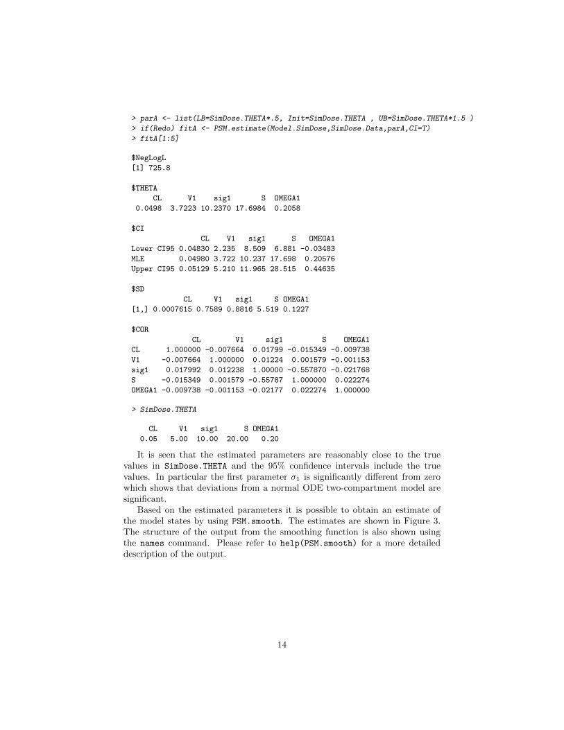
> parA <- list(LB=SimDose.THETA*.5, Init=SimDose.THETA , UB=SimDose.THETA*1.5 )
> if(Redo) fitA <- PSM.estimate(Model.SimDose,SimDose.Data,parA,CI=T)
> fitA[1:5]
$NegLogL
[1] 725.8
$THETA
CL V1 sig1 S OMEGA1
0.0498 3.7223 10.2370 17.6984 0.2058
$CI
CL V1 sig1 S OMEGA1
Lower CI95 0.04830 2.235 8.509 6.881 -0.03483
MLE 0.04980 3.722 10.237 17.698 0.20576
Upper CI95 0.05129 5.210 11.965 28.515 0.44635
$SD
CL V1 sig1 S OMEGA1
[1,] 0.0007615 0.7589 0.8816 5.519 0.1227
$COR
CL V1 sig1 S OMEGA1
CL 1.000000 -0.007664 0.01799 -0.015349 -0.009738
V1 -0.007664 1.000000 0.01224 0.001579 -0.001153
sig1 0.017992 0.012238 1.00000 -0.557870 -0.021768
S -0.015349 0.001579 -0.55787 1.000000 0.022274
OMEGA1 -0.009738 -0.001153 -0.02177 0.022274 1.000000
> SimDose.THETA
CL V1 sig1 S OMEGA1
0.05 5.00 10.00 20.00 0.20
It is seen that the estimated parameters are reasonably close to the truevalues in SimDose.THETA and the 95% confidence intervals include the truevalues. In particular the first parameter σ1 is significantly different from zerowhich shows that deviations from a normal ODE two-compartment model aresignificant.
Based on the estimated parameters it is possible to obtain an estimate ofthe model states by using PSM.smooth. The estimates are shown in Figure 3.The structure of the output from the smoothing function is also shown usingthe names command. Please refer to help(PSM.smooth) for a more detaileddescription of the output.
14

> if(Redo)
+ out <- PSM.smooth(Model.SimDose, SimDose.Data, fitA$THETA, subsample = 20)
> # View the data structure
> names(out[[1]])
[1] "Time" "Xs" "Ps" "Ys" "Xf"
[6] "Pf" "Xp" "Pp" "Yp" "R"
[11] "eta" "negLogL"
By comparing the smoothed estimates of the states to the true simulatedstates, it can be seen that they are very close. This shows that the system noiseand observation noise has been separated properly in the reconstruction.
0 100 200 300 400
020
040
060
0
Individual 1
SimDose.Data[[id]]$Time
Obs
erva
tions
Smooth est.
0 100 200 300 400
050
010
0015
00
SimDose.Data[[id]]$longTime
Sta
te 1
SimulationSmooth est.
0 100 200 300 400
040
080
012
00
Sta
te 2
SimulationSmooth est.
0 100 200 300 400
050
100
150
200
Individual 2
SimDose.Data[[id]]$Time
Obs
erva
tions
Smooth est.
0 100 200 300 400
050
010
0015
00
SimDose.Data[[id]]$longTime
Sta
te 1
SimulationSmooth est.
0 100 200 300 400
020
060
010
00
Sta
te 2
SimulationSmooth est.
Figure 3: Smoothed estimate of states.
15

5.2 Extraction of insulin secretion rate (Linear)
Insulin secretion rates (ISR) can be estimated based on measurements of theconcentration of C-peptide in the blood, since insulin and C-peptide are secretedin equi-molar amounts. This example will first illustrate a way to simulate C-peptide data based on a model for ISR, and then how ISR can be estimated againusing a more simple model. The models used in the example are described infurther detail in [5].
The simulated measurements of C-peptide spans over 24H, during which thepatients recieves three meals at 8 a.m., 12 a.m. and 6 p.m. These meals will giverise to an increase in insulin secretion, which will be modelled and estimated.
The simulation model for the C-peptide measurements is based on the com-monly used two compartment model for C-peptide as shown in Figure 4. Thekinetic parameters are set equal to the Van Cauter estimates [6].
ke k2
k1
C2C1
ISR
Figure 4: Model layout
The first two states of the simulation model is concentration in compartment1 and 2, C1, C2. The third state is ISR and is the secretion which is modelledas a structural part based on the three meal time plus a constant baseline B andrandom noise through a Wiener process. The fourth state Q is used to modelISR, where Q is controlled by an input u2 which is equal to 1 for 30min aftermeal times. The model can be defined as
dC1 = [−(k1 + ke)C1 + k2C2 + ISR]dt (19)
dC2 = [k1C1 − k2C2]dt (20)
dISR = [−a1ISR+ a1Q+Bi]dt+ σISRdω (21)
dQ = [−a2Q+ a2Kiu2]dt (22)
which is linear and can thus again be written on matrix form.The model is initialized in steady state just prior to the first meal time. The
individual variation in the model is included in the initial concentration C1(0)i,baseline Bi and height of the peaks Ki such that
Bi = B exp(η1) (23)
Ki = K exp(η2) (24)
C1(0)i = C1(0) exp(η3) (25)
16

In order to write a model containing a constant in the differential equations(here Bi) on the linear form as defined in Eq. (2) and (3) it is necessaryto include a constant input u1 = 1 and multiply this with Bi. The matrixdescription of the model can be found in [5] p. 69. Using this, the model canbe defined in PSM as follows.
17

> k1 = 0.053; k2 = 0.051; ke = 0.062;
> Model.SimISR <- list()
> Model.SimISR$Matrices = function(phi)
+ a1 <- phi[["a1"]]
+ a2 <- phi[["a2"]]
+ B <- phi[["B"]]
+ K <- phi[["K"]]
+ matA <- matrix( c(-(k1+ke) , k2 , 1 , 0,
+ k1 , -k2 , 0 , 0,
+ 0 , 0 , -a1 , a1,
+ 0 , 0 , 0 , -a2),nrow=4,byrow=T)
+ matB <- matrix( c(0 , 0 ,
+ 0 , 0 ,
+ B , 0 ,
+ 0 , a2*K),byrow=T,nrow=4)
+ matC <- matrix(c(1,0,0,0),nrow=1)
+ matD <- matrix(c(0,0),nrow=1)
+ list(matA=matA,matB=matB,matC=matC,matD=matD)
+
> Model.SimISR$X0 = function(Time=NA,phi,U=NA)
+ C0 <- phi[["C0"]]
+ tmp <- C0
+ tmp[2] <- C0*k1/k2
+ tmp[3] <- C0*ke
+ tmp[4] <- 0
+ matrix(tmp,ncol=1)
+
> Model.SimISR$SIG = function(phi)
+ diag( c(0,0,phi[["SIG33"]],0))
+
> Model.SimISR$S = function(phi)
+ return( matrix(phi[["S"]]))
+
> Model.SimISR$h = function(eta,theta,covar)
+ phi <- theta
+ phi[["B"]] <- theta[["B"]]*exp(eta[1])
+ phi[["K"]] <- theta[["K"]]*exp(eta[2])
+ phi[["C0"]] <- theta[["C0"]]*exp(eta[3])
+ return(phi)
+
> Model.SimISR$ModelPar = function(THETA)
+ list(theta=list(C0=900,S=8500,
+ a1=THETA[’a1’],a2=THETA[’a2’],
+ SIG33=THETA[’SIG33’],
+ K = THETA[’K’], B = THETA[’B’]),
+ OMEGA=diag(c(.2,.2,.2))
+ )
+
>
For this example two individuals will be simulated. They will both be sam-
18

pled at predefined time points during 24H. This defined as below together withthe input data for each individual.
> Sim.Data <- vector(mode="list",length=2)
> for (i in 1:2)
+ Sim.Data[[i]]$Time <- c( 0,15,30,45,60,75,90,120,150,180,210,240,270,300,330,
+ 360,420,480,600,615,630,645,660,675,690,720,750,780,810,
+ 840,960,1140,1320,1410,1440)
+ Sim.Data[[i]]$U <- matrix(c( rep(1,35) ,
+ as.numeric( Sim.Data[[i]]$Time %in% c(0,15,240,600,615)) )
+ ,byrow=T,nrow=2)
+
Both the model, sample times and input is now prepared and the simulationcan be performed. The parameter estimates are taken from [5] p. 70. Thesimulated data are shown in Figure 5.
> Sim.THETA <- c(a1=0.02798, a2=0.01048, SIG33=4 , K=427.63 , B=1.7434)
> if(Redo)
+ Sim.Data <- PSM.simulate(Model.SimISR, Sim.Data, Sim.THETA, deltaTime=.1 )
+ else
+ load("simisr.RData")
The next step is to generate a model for estimation of ISR. It is again basedon the model illustrated in Figure 4 only this time the ISR is simply modelledas a random walk. Thus no information about the meal times is used in theestimation of ISR.
The model simplification is done by replacing Eq. (21) and (22) by Eq. (26)below. The model for estimation can thus be seen as estimating the outcome ofthe random walk for ISR based on the observed (simulated) data for C1.
dISR = σISR (26)
19

0 200 400 600 800 120050
015
00
Sim.Data[[id]]$longTime
Sta
te 1
Individual 1, eta=(−0.556,0.104,0.538)
Obs.
0 200 400 600 800 1200
500
1500
Sim.Data[[id]]$longTime
Sta
te 2
0 200 400 600 800 1200
050
150
Sim.Data[[id]]$longTime
Sta
te 3
0 200 400 600 800 1200
040
8012
0
Sta
te 4
0 200 400 600 800 1200
500
1500
Sim.Data[[id]]$longTime
Sta
te 1
Individual 2, eta=(−0.192,−0.189,−0.343)
Obs.
0 200 400 600 800 1200
600
1200
1800
Sim.Data[[id]]$longTime
Sta
te 2
0 200 400 600 800 12000
5010
015
0
Sim.Data[[id]]$longTime
Sta
te 3
0 200 400 600 800 1200
040
80
Sta
te 4
Figure 5: Simulated data and states.
> Model.Est <- list(
+ Matrices=function(phi) list(
+ matA=matrix(c(-(k1+ke), k2, 1,
+ k1 , -k2, 0,
+ 0 , 0, 0 ),ncol=3,byrow=T),
+ matB=NA,
+ matC=matrix(c(1,0,0),nrow=1),
+ matD=NA ) ,
+ X0 = function(Time=NA,phi=NA,U=NA)
+ C0 <- phi[["C0"]]
+ tmp <- C0
+ tmp[2] <- C0*k1/k2
+ tmp[3] <- C0*ke
+ return(matrix(tmp,ncol=1) ) ,
+ SIG = function(phi)
+ return( diag( c(1e-3,1e-3,phi[["SIG33"]])) ) ,
+ S = function(phi)
+ return( matrix(phi[["S"]])) ,
+ h = function(eta,theta,covar)
+ phi <- theta
+ phi[["C0"]] <- theta[["C0"]]*exp(eta[1])
+ return(phi) ,
+ ModelPar = function(THETA)
+ return(list(theta=list(C0=THETA[’C0’],S=THETA[’S’],SIG33=THETA[’SIG33’]),
+ OMEGA=matrix(THETA[’OMEGA’])))
+ )
20

Looking at the ModelPar-function it is seen that it is chosen to include theaverage initial concentration C1(0), measurement variation S, the coefficient ofthe random walk for ISR σISR and the variance of the random effect on C1(0)denoted ΩC1(0) in the likelihood estimation.
Since the model now does not use any input, this must be removed from thesimulated data before estimation.
> Pop.Data <- Sim.Data
> for (i in 1:2)
+ Pop.Data[[i]]$U <- NULL
The data and model for estimation is now prepared, and the model canbe estimated by calling PSM.estimate. This is done below and the output inobj1[1:3] containing the log-likelihood value, parameter estimates and confi-dence intervals is shown as output.
> par1 <- list(LB = c(C0= 200, S= 50^2, SIG33= 0, OMEGA=.0 ),
+ Init = c(C0=1000, S=100^2, SIG33=10, OMEGA=.25),
+ UB = c(C0=3000, S=150^2, SIG33=15, OMEGA=.50))
> if(Redo) obj1 <- PSM.estimate(Model.Est, Pop.Data, par1,CI=T,trace=1)
> obj1[1:5]
$NegLogL
[1] 497.6
$THETA
C0 S SIG33 OMEGA
1.121e+03 1.023e+04 4.768e+00 1.464e-01
$CI
C0 S SIG33 OMEGA
Lower CI95 490.8 2265 3.556 -0.1717
MLE 1121.1 10227 4.768 0.1464
Upper CI95 1751.5 18188 5.979 0.4645
$SD
C0 S SIG33 OMEGA
[1,] 321.6 4062 0.6181 0.1623
$COR
C0 S SIG33 OMEGA
C0 1.00000 -0.03063 0.03367 -0.09409
S -0.03063 1.00000 -0.39152 0.04218
SIG33 0.03367 -0.39152 1.00000 -0.05177
OMEGA -0.09409 0.04218 -0.05177 1.00000
Looking at the estimated confidence intervals, it is seen that the values usedin the simulation Θ = (900,8500,4,0.2) are nicely contained within the limits.
The estimation time including the confidence interval is about 3 minuteson a 2GHz computer. Since the matrix A in the estimation model is singular,
21

the estimation cannot make use of the compiled Fortran code. As mentioned,this may be circumvented by adding e.g. 10−6 to the diagonal. This reducesthe estimation time to 12 sec. It changes the maximum log-likelihood value to499.4781, and thus yields virtually no difference in parameter estimates.
Using the estimated model parameters it is possible to give smoothed esti-mates of the three model states C1, C2 and ISR. This is done below and theresult is plottet in Figure 6. In Figure 7 the smoothed ISR state is plottedtogether with the estimated uncertainty. For both figures the true simulatedstates is also plotted for reference.
> if(Redo)
+ Data.Sm <- PSM.smooth( Model.Est , Pop.Data, obj1$THETA, subsample=10)
0 200 400 600 800 1200
500
1500
Individual 1
Sta
te 1
Simul.Sm. est.
Individual 1
0 200 400 600 800 1200
500
1500
Individual 1
Sta
te 2
Simul.Sm. est.
0 200 400 600 800 1200
050
150
Individual 1
Sta
te 3
Simul.Sm. est.
0 200 400 600 800 1200
040
8012
0
Sta
te 4
Simul.Sm. est.
0 200 400 600 800 1200
500
1500
Individual 2
Sta
te 1
Simul.Sm. est.
Individual 2
0 200 400 600 800 1200
600
1200
1800
Individual 2
Sta
te 2
Simul.Sm. est.
0 200 400 600 800 1200
050
100
150
Individual 2
Sta
te 3
Simul.Sm. est.
0 200 400 600 800 1200
040
80
Sta
te 4
Simul.Sm. est.
Figure 6: Smoothed estimate of states.
22

0 200 400 600 800 1000 1200 1400
050
100
150
minutes
pmol
/min
SimulationSmooth est.
0 200 400 600 800 1000 1200 1400
040
8012
0
minutes
pmol
/min
SimulationSmooth est.
Figure 7: Smoothed estimate of insulin secretion rate ±1SD for individual 1 and2 compared with the true simulated ISR.
References
[1] Mortensen SB, Klim S, Dammann B, Kristensen NR, Madsen H, Overgaard RV(2007) A Matlab framework for estimation of nlme models using stochastic dif-ferential equations: applications for estimation of insulin secretion rates. J ofParmacokinet Pharmacodyn 34:623-642
[2] Overgaard RV, Jonsson N, Tornøe CW, Madsen H (2005) Non-linear mixed-effectsmodels with stochastic differential equations: implementation of an estimationalgorithm. J of Parmacokinet Pharmacodyn 32(1):85-107
[3] Kristensen NR, Madsen H (2003) Continous time stochastic modelling: CTSM2.3 mathematics guide, Technical University of Denmarkhttp://www2.imm.dtu.dk/ctsm/MathGuide.pdf
[4] Beal SL, Sheiner LB (2004) NONMEM R©Users Guide. University of California,NONMEM Project Group.
[5] Klim S, Mortensen SB (2006) Stochastic PK/PD Modelling. M.Sc. thesis,Informatics and Mathematical Modelling, Technical University of Denmark.http://www2.imm.dtu.dk/pubdb/views/edoc download.php/4533/pdf/imm4533.pdf
[6] Van Cauter E, Mestrez F, Sturis J, Polonsky KS (1992) Estimation of insulinsecretion rates from C-peptide levels. Comparison of individual and standardkinetic parameters for C-peptide clearance. Diabetes, 41(3), pp. 368-77.
23