portable xrf: a very brief introduction

Drake, L. (2016), Portable XRF: A (very) brief introduction. In: Homem, P.M. (ed.) Lights On…

Cultural Heritage and Museums!. Porto: LabCR | FLUP, pp.140-161

140

1 Bruker, US, University of New Mexico, US, [email protected]

PORTABLE XRF: A (VERY) BRIEF

INTRODUCTION Lee Drake1

ABSTRACT The growth of portable x-ray fluorescence instruments (pXRF) have challenged traditional analytical protocols, primarily in its use in non-destructive contexts.

The present manuscript evaluates the ways that pXRF differs from traditional laboratory XRF, and the limitations and opportunities which emerge from this difference. Both qualitative and quantitative uses are illustrated with a focus on applications for cultural heritage management.

KEYWORDS Portable X-Ray Fluorescence; Methodology; Qualitative; Quantitative



141

Perception of visible light

The perception of colors, from the reds of the thin, subtle smile in Da

Vinci’s Mona Lisa to the blue sky of Picasso’s Starry Night, owe a debt

to the evolution of our primate ancestors. While most mammals can

clearly see blue and red, the ability to differentiate lower-

energy/longer wavelength colors is rare. In the deep past, the primate

ancestors of humans were dependent on differentiating red from

green to find fruit in dense jungle stands - this created a powerful

selective force which gave primates a broader spectrum than most

other mammals (Regan et al. 1998). As can be seen in FIG. 1, the long

and medium cone cells, responsible for red and green, have very subtle

differences in sensitivity to different photon energies, as can be seen

in FIG. 1. Our ability to see green may be due to a gene duplication

event with some mutation that formed the M-cone from the L-cone

(Nathans and Thomas, 1986).

Despite the closeness of energy sensitive, the eyes of modern humans

are generally capable of differentiating between multiple hues

between red and green, giving the world, and art, its richness of

experience. It is important to underline here that the color range of

humans, which extends from 1.7 to 3.1 electron volts (eV) of energy

FIG. 1 - Cone cell energy

sensitivity (Stockman et

al., 1993).



142

(700 - 300 nanometers), is a product of our unique evolutionary

history. Our perception of the world is confined to these limits. Other

organisms have colors which exceed the unusually broad and detailed

spectrum humans enjoy; some species of honeybees can see into the

ultraviolet (UV) range, while others such as snakes perceive in the

infrared (IR) range.

Outside the visible spectrum

The developments in instrumental science over the past several

decades have used increasingly sophisticated light generators and

detectors to make the known entirety of light’s spectrum available to

humans for study, from radio waves with 100 km wavelengths

(1.2398e-11 eV) to the gamma rays of supernova of 300 keV (0.0004

nm wavelength). As such, the concept of color expands dramatically

when we consider these higher and lower energy photons.

Miniaturization of components have taken formerly large laboratory-

confined instruments into smaller, handheld devices (Bostco, 2013).

This displacement from the lab has led to the use of handheld

instrumentation in contexts which present unique challenges and

opportunities. This paper concerns itself primarily with handheld x-ray

fluorescence (pXRF) spectrometers, however the principles of matrix

effects and attenuation will affect other types of instrumentation as

well.

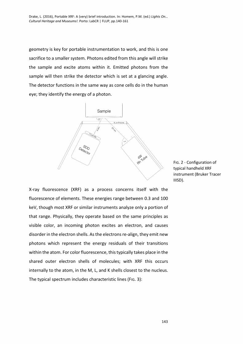
XRF instruments (FIG. 2) attain their portability by using geometry to

fit key components in small spaces. An X-ray tube is configured at a 52°

angle relative to the nose of the instrument. This is not the best

geometry of an XRF instrument, an angle of 90° is preferable for

maximum limits of detection (Klockenkaemper, 1997). However, the



143

geometry is key for portable instrumentation to work, and this is one

sacrifice to a smaller system. Photons edited from this angle will strike

the sample and excite atoms within it. Emitted photons from the

sample will then strike the detector which is set at a glancing angle.

The detector functions in the same way as cone cells do in the human

eye; they identify the energy of a photon.

X-ray fluorescence (XRF) as a process concerns itself with the

fluorescence of elements. These energies range between 0.3 and 100

keV, though most XRF or similar instruments analyze only a portion of

that range. Physically, they operate based on the same principles as

visible color, an incoming photon excites an electron, and causes

disorder in the electron shells. As the electrons re-align, they emit new

photons which represent the energy residuals of their transitions

within the atom. For color fluorescence, this typically takes place in the

shared outer electron shells of molecules; with XRF this occurs

internally to the atom, in the M, L, and K shells closest to the nucleus.

The typical spectrum includes characteristic lines (FIG. 3):

FIG. 2 - Configuration of

typical handheld XRF

instrument (Bruker Tracer

IIISD).



144

In this case, each element fluoresces with unique peaks - Potassium

(K) has a K-alpha line at 3.55 keV, and a K-beta peak at 3.60 keV. These

can be thought of as the colors of Potassium, if red is 1.7 eV and blue

3.0 eV, then Potassium’s K-alpha line is a color at 3,550 eV.

Again, the XRF spectrum is an extension of our color vision, something

which enables us to see more than the colors our primate ancestors

left us with. The big difference is what we see - with visible color

fluorescence it is the molecules which fluoresce. For example, reduced

iron (Fe2+) looks black to us, because all visible photons are absorbed.

If it is oxidized to hematite (Fe2O3) then we would see an orange-red

color. This is because photons of an energy of 1.7 - 1.9 eV are emitted

from the shared outer electron shells of the molecule following light’s

absorption.

To an XRF unit, the Fe K-alpha and K-beta lines (6.4 and 6.9 keV,

respectively) would fluoresce just the same - the arrangement in the

outer electron shells does not affect the absorption or emission

energies of those orbitals closest to the nucleus. As such, XRF is

primarily a method to detect elements.

FIG. 3 - XRF spectrum of

NIST 1547, Apple Mango

Leaves.



145

The XRF spectrum

The XRF spectrum is most typically used in the identification and/or

quantification of elemental fluorescence peaks. However, there are

multiple other types of photon interaction present than simple

fluorescence.

In FIG. 4, numerous other peaks manifest in the spectrum. These

include the Rayleigh peak, which is formed by elastic scatter of

photons from the XRF tube. These will have an energy that matches

the K-alpha (or L-alpha) line of the x-ray target.

They are formed when photons leave the tube and are reflected by the

sample without losing any energy - they are the parallel for white light

in this portion of the spectrum. The Rayleigh peak is situated between

two Compton peaks, one at a lower energy at another at a higher

energy. These are the inelastic scatter that results from photons with

the energy of the XRF target (e.g. same as Rayleigh) but they loose (or

gain) energy on their way back to the detector. The ratio of the lower-

energy Compton peak to Rayleigh will correspond to the density of the

electron cloud (e.g. higher ratio with lighter elements). These three

peaks overlay a broader set of photon counts, collectively known as

Bremsstrahlung radiation. These are the x-ray photons which simply

FIG. 4 - Spectrum of a

diamond taken with a 25

μm Ti/300 μm Al filter and

a rhodium (Rh) tube.



146

bounce around in the matrix of the material and loose energy - they

are informally known as the backscatter. To the left, the backscatter

does not mirror its counterpart to the right, it has a bowl-curve

descending to 0 counts per second. This is the consequence of adding

a filter, which eliminates a portion of the spectrum. This is typically

done to increase the signal-to-noise ratio of elements with fluoresce

in a given region.

Peaks fluoresce in the spectrum based on the quantity of atoms

present and the luminescence settings of the instrument used. Just as

with color fluorescence, more energy must be sent than is returned.

Each element has a range of photons which can excite electrons in its

K, L, and M orbitals. There is a terminal point at which a certain photon

can no longer excite these orbitals for a given element, this is known

as the absorption edge. This point is also the point of maximum

excitation potential, the effectiveness of a photon to excite the

element in question declines with higher energies. The overall

potential of excitation looks something like a Gaussian distribution

which was cut in half (FIG. 5).

The fewer photons there are to the right of the absorption edge, the

smaller the chance of fluorescence there is. The converse is also true,

FIG. 5 - Absorption Edge of

Rubidium (Rb).



147

the more photons on the absorption edge, the higher the chance of

fluorescence. Filters can be used to increase or decrease the chance of

an element fluorescing, but ultimately the ability to seen an element

rests with the sample.

What makes pXRF different?

For decades, laboratory XRF units have been highly reliable systems

with straightforward quantification. However, portable XRF

instruments are much more difficult to use quantitatively (Frahm,

2013). The components between the two are the same, why would

portable XRF underperform? The reason has less to do with the

configuration of the XRF and more to do with the sample. Laboratory

XRF units typically analyze prepared samples, usually fused glass

beads. This means samples have been homogenized and prepared for

analysis - this also means the matrix (in this case SiO2) matches that of

the reference standards of the equipment. Portable XRF, in contrast,

is used in situations where samples are not prepared. In fact, the use

of pXRF is frequently on heterogenous samples. As such, the

limitations stem not from the physical components but rather the use

of the system to analyze paintings, ceramics, and other heterogenous

objects in a non-destructive manner (Kaiser and Shugar, 2012). That

said, when samples are prepared the same way, portable

instrumentation can have equal performance to laboratory equipment

(Guerra et al., 2014).

This means, in short, that matrix effects are essential considerations in

the use of portable XRF. Some elaboration may be needed on the term

matrix; this simply refers to the majority material by composition. The

matrix of soil would be SiO2, the matrix of stainless steel would be a



148

crystalline mixture of Fe, Cr, and Ni. The matrix affects the spectrum in

two primary ways, the first is by affecting the depth of analysis.

The depth of analysis is the product of the mass attenuation of

photons as they enter any matrix, be it gas, liquid, or solid. The atoms

of the matrix gradually absorb photons. The denser the matrix, the

more rapid this loss of photons is. Photons with higher energies will be

able to make it further into the matrix. The relationship can be

expressed as follows:

I/I0 = e[-(μ/ρ)ρ]

where I is the quantity of photons returning from the sample, I0 is the

quantity of photons entering the sample, μ/ρ represents the mass

attenuation coefficient of a given element for a particular matrix, and

ρ represents the density of the object. Assuming only 1% of photons

return from a sample, the equation can be reduced to:

depth (cm) = 4.61/(-μ/ρ*ρ)

In this case, the depth of analysis for a silicate can be calculated (FIG.

6):

For light elements, such as Si, the analytical depth is only 27 μm for the

K-alpha peak. For heavier elements, such as the K-alpha emission for

FIG. 6 - Depth of analysis

for a silicate by photon

energy.



149

Fe, it can be 300 μm deep. The L-line for Pb would be 1,130 μm, and

Ag’s K-alpha peak can be seen at a depth of over 200,000 μm, or 2 cm,

deep. As such, the spectrum will produce a biased view of different

elements depending on their energy.

Second, the presence of new elements can influence the fluorescence

of others as they can overly each other’s absorption edges.

In FIG. 7, Fe sits on the absorption edge of Ti, which in turn sits on the

absorption edge of S.

In this case, each element heightens the fluorescence of an element of

lower energy. And in turn, each element of lower energy reduced the

height of the higher energy peak lying in its absorption edge. An Fe K-

alpha photon can be emitted, then strike a Ti atom, which in turn emits

a Ti K-alpha photon, which is absorbed by S. This highlights the

resonance effect which takes place in elemental spectra. As an

analogy, the spectrum can be thought of as a symphony, and each

element an instrument. As the violins swell, the clarinet deepens. The

user of portable XRF equipment can conduct analysis more effectively

by shaping the energy, current, filter, and even atmosphere that the

analysis is taken in to accentuate the fluorescence of elements.

FIG. 7 - Absorption edges

for S, Ti, and Fe.



150

As mentioned before, laboratory instruments also deal with these

physical phenomenon, but in a controlled setting. They standardize

the matrix, and can be calibrated to a higher degree. Portable

instrumentation is much more vulnerable to matrix effects because

the sample analyzed are typically heterogenous and unprepared.

While this is a sacrifice from the point of view of spectrum quality, it is

an advantage in that it is non-destructive. A painting can be painlessly

analyzed using XRF, while in most cases the homogenization of the

pigments into a fused glass bead are unpalatable. It is important to

note, in non-destructive uses of the equipment, that matrix effects not

be taken for granted. It is important for spectra to be assessed

qualitatively given these conditions.

Qualitative analysis

The utility in art conservation for XRF consists in expanding our

spectrum to see those elements which are compositionally important

to a piece of art or a heritage object. For conservation, XRF can be used

to identify elements or materials which may not be consistent with the

point of origin of an object, identifying potentially reactive elements,

or to analyze variation in the composition, among other tasks. In

general, any analysis first needs context. For example, analysis of a

historical painting means that a certain set of pigments are expected

for its point of composition. A Rembrandt painting will include

historical pigments such as lead white (PbCO3), vermillion (HgS) and

bone black (CaPO4) based on their availability during the time in which

he was alive. If a synthetic pigment base such as titanium dioxide (TiO2)

or zinc oxide (ZnO) is present, then the painting is either retouched, or

is not secure in its provenance. Likewise, the identification of calcite

(CaCO3) or gypsum (CaSO4) could indicate the presence of the recent,



151

reversible restoration. In either case, the context of the object is

inseparable from the interpretation of XRF spectra - neither exists in

isolation.

A similar example can exist with heritage objects. In North America,

pre-Colombian cultures rarely used anything other than pure copper

or gold as metals. An XRF spectrum of these objects should produce

pure K lines for Cu or L lines for gold, with the potential for small

impurities like Ag and Pb. The presence of a substantial amount of Zn

or Sn would indicate a brass or bronze alloy, technology with had no

president prior to the arrival of the Spanish in 1492.

Note that in these two examples XRF does not need to be used

quantitatively to answer a straightforward question: do we

understand the object’s place in time? Qualitative analysis is sufficient

to answer this question. The qualitative analysis of XRF spectra is, in

essence, the same as qualitative analysis performed with human eyes

- no further elaboration is always needed when describing a color such

as red. In the same sense, no further elaboration is needed when a

brass object shows up in a prehistoric collection - it is impossible for it

to be both brass and prehistoric.

Complications to qualitative analysis

The intensity of the K-, L-, and M- peaks in an XRF spectrum

corresponds to the relative abundance of that element give the

fluorescence parameters (energy, filter, atmosphere, etc.). The

spectral peaks can be thought of as proxies for atoms themselves,

though there are some basic factors that complicate this picture (FIG.

8).



152

By atomic abundance, sodium chloride is 50% Na and 50% Cl. So, why

is the Cl K-alpha peak magnitudes of order higher than the Na peak?

There are three reasons why:

1. The depth of analysis of Cl is 38 μm, while Na is 5μm;

2. Cl is closer to the medium of the Brehmsstralung radiation, while

Na at the tail;

3. Cl has a fluorescence efficiency of 9%, while Na has a fluorescence

efficiency of 2%.

As such, there are few photons to fluoresce Na, which in turn

fluoresces less efficiently, and at a shallower depth than Cl. These

factors combine to dramatically reduce the Na K-alpha peak. The first

two factors have been covered earlier in this manuscript, the latter is

in need of further elaboration. Fluorescence efficiency refers to how

many atoms out of 100 will fluoresce in a given electron orbital if a

photon has the necessary energy. This efficiency is determined by the

number of electrons in the outer orbitals and the repulsive charges

they have on each other. A lower number means less atoms will light

up; a higher number means more. Typically, the more electrons in the

outer orbitals, the more likely a K-alpha or L-alpha emission will occur.

FIG. 8 - Spectrum of

sodium chloride taken

using a helium flush. The

small peak to the left of

the Na K-alpha peak is the

escape peak for Cl.



153

Because Na is a lighter element than Cl, there are less candidates for

the transfer.

For these reasons, the spectral peaks cannot be considered perfect

proxies for atomic counts - there are many biases at work that affect

the fluorescence of elements, not all of which can be controlled by the

user. That said, if fluorescence parameters, or illumination, is kept

constant from sample to sample (e.g. same energy, current, filter,

time, and atmosphere) then peaks of the same element in different

samples will vary based on their concentrations/atomic abundances.

Quantitative analysis

Typically, we tend to think about the presence of elements in material

in terms of concentrations, e.g. 7% Fe, 325 ppm Rb. These percentages

refer to either volume or, more commonly, weight. However, the use

of weight percent to characterize material can sometimes obscure its

composition somewhat. Take our earlier example of salt. It is 50% Na

and 50% Cl by atomic abundance, captured by its chemical formula

NaCl. However, Na has 11 protons while Cl has 17. This means that Na

has an atomic weight (with common isotopes included) of 22.99 while

Cl has one of 35.45. Cl thus weights 54% more than Na. As such, NaCl

is by weight 39% and Cl 61%. Think about the contradiction there for

just a moment - while there are just as many atoms of Na and Cl in salt

the latter is a greater weight percent than the former. Phrasing

composition in the context of weight conflates two different points of

variation - the atomic abundance of an element and its atomic weight.

A more dramatic example can be seen with water, H2O. H has an

atomic weight of 1 while O has an atomic weight of 16. There are twice

as many H atoms as there are of O, yet those H atoms compose roughly

11% of water’s weight.



154

The prominence of weight % in chemical composition analysis owes to

the history of chemistry. In the classical and medieval eras, there were

two major branches of chemistry, the first being alchemy (the

attempts to transform elements into gold) and the second being

metallurgy (the process of creating tools, weapons, and structures).

Both carefully weighed out ingredients prior to incorporation into

materials and experiments. For example, a metallurgist would add 1

kg Sn for every 9 kg Cu to create a bronze sword. This tradition carried

over into modern material science in most cases, remaining the

standard by which we analyze objects today.

From the perspective of XRF, a major complication is added - the

traditional units of composition are not directly reflected in the atomic

spectrum. To perform quantitative analysis - specifically in terms of

weight percent - some kind of calibration is needed. There are two

primary mathematical approaches to doing this. The first is to use

fundamental parameters of the instrumentation to create estimates

of an item’s composition. This includes the angle of the x-ray tube, the

glancing angle of the detector, the space from the sample to the

detector, and assumptions about composition. If dealing with a sample

in which 100% of the atoms fluoresce in range of the tube and

detector’s capabilities, this approach can work quite well because all

points of variation can be included. If, however, not all elements can

be seen, then the situation becomes much more complicated. For

example, a piece of glass is, by both weight and volume, mostly O.

EDXRF cannot detect this element - even if it could it would only be at

a depth of 10 nm in the sample. FP algorithms must from this point

make a guess about the elements it cannot see to estimate the weight

percent of Fe, Cu, Zn, and other metals. The inability to see Na without

atmospheric changes further complicates the task. Though glass



155

represents a partially synthetic material, SiO2 and Al2O3 are dominant

and oxygen can be extrapolated from there. Soils and ceramics are

much more challenging. There are multiple forms for Ca, including

CaSO4, CaPO4, CaO, CaCO3, etc. There are two common oxidization

states for Iron, Fe2O3, FeO, etc. FP algorithms work best with highly

synthetic substances such as metals in which all elements present can

be excited by the instrument. An example is the Rosseau (2009) FP

algorithm:

Ci = Ri ((1 + ΣjAijCj)/(1+ΣjεijCj))

where Ci represents the concentration of an element, Ri is the relative

intensity of an element, aij are the absorption coefficients, Cj

represents the element at concentration, and εij represents the

enhancement coefficients. Determination of aij and εij require

information on total matrix composition - thus the algorithm only

functions if a prior is given to it (e.g. information about the sample).

For proper FP calculation, additional information about the tube and

detector geometry/distance is needed, such as those details

documented in FIG. 2.

The second major method to quantify XRF spectra is to use reference

standards, these are known as empirical calibrations. The approach of

an Empirical calibration is most commonly a variant of the common

linear model developed by Lukas-Tooth and Price (1961):

Ci = r0 + Ii(ri + Σrin+In)

Where Ci represents the concentration of element, r0 is the

intercept/empirical constant for element i, ri - slope/empirical

coefficient for intensity of element i, rn is the slope/empirical constant

for effect of element n on element i, Ii is the net intensity of element I,



156

and In is the net intensity of element n. This equation descends from a

simple linear model,

y = mx + b

In which y is Ci, b is r0, m is ri, and Ii is x (eg. Ci = riIi + r0). The additional

variables present in the Lukas-Tooth equation indicate a slope

correction for an element which influences the fluorescence of the

element to be analyzed (subscript i represents the element being

analyzed, subscript n represents the influencing element). An

illustration of how this effect occurs can be seen in FIG. 7. Here, the K-

alpha peak of Fe overlays the absorption edge for the K-alpha emission

of Ti. In this circumstance, the quantification of Ti may use Fe as a slope

correction. While the Lukas-Tooth method of quantification has been

criticized for being a brute-force statistical quantification approach,

physical principles can be used to guide the application of corrections.

It is important, however, to strive for minimalism in these

quantifications. Too many corrections can artificially increase the r2

value of a linear/non-linear model. Unrelated corrections will inflate

the perceived accuracy of the model; real world application will

increase the chance of a violation to its generalizability. The fewer

corrections, the more generalizable the model. An additional benefit

is that violations to a simple Empirical Calibration can result in

systematic error as opposed to random error (Nazaroff et al., 2010).

By using matrix-specific calibrations, almost any material can be

quantified using EDXRF data (Speakman and Shackley, 2013). FIG. 8

shows a simple empirical calibration built for ppm-levels of Pb in water

in this case, 10,000 ppm of a reference standard (Lead, 10,000 ppm,

ICP Standard Solution) was titrated down to 1ppm using repeat half-

dilutions with distilled water (FIG. 9).



157

This calibration represents the simplistic possible implementation of a

calibration, in which there are no overlapping peaks. Note that even in

this case the effect is beyond a simple linear model; a quadratic

formula was used due to the effects of depth on the analysis.

Calibration curves become more complicated as different overlapping

elemental lines influence the curve. The Lukas-Tooth and Price

equation will turn these into multilinear models - thus creating multi-

dimensional calibration curves that cannot easily be displayed in a

bivariate plot. Nonetheless, the principles are simple and

straightforward.

Layer thickness and position

XRF has one highly unique application in which non-destructive

analysis provides more detailed information than simple

concentrations. In the right circumstances, it can be used to predict

the thickness of an object with micron-level accuracy. This is a

consequence of two factors in XRF; the first is that there are multiple

peaks for each element at different energies, the second is that higher

energy photons penetrate greater depths of a material. To return to

FIG. 9 - Pb in water

empirical calibration.



158

the example of Pb, it has two primary L peaks, an L-alpha at 10.5 keV

and an L-beta at 12.5 keV. The attenuation of the L-alpha peak will be

greater in every matrix than the L-beta since it has 20% less energy.

This means that as the L-beta peak rises relative to the L-alpha peak,

the depth of the surface covering must also increase. FIG. 10 illustrated

this effect with different thicknesses of pure Al foil, ranging from 0 to

775 μm Al overlaying pure Pb.

This principle can be used to identify surface coverings - indeed an

entire industry of coating thickness analyzers exists based on this

principle. The same principle holds true for any conceivable layering;

varnishes on a painting, pigments on top of other pigments, metal

plating on other metal. The analysis can be done spectrally, provided

that a surface-level reading of the low layer is available. An example of

this is the spectrum of Pb in Figure 9: The smallest L-beta represents

the surface-level measurement of Pb; the L-beta/L-alpha ratio here is

about 0.85. By contrast, the L-beta/L-alpha ratio for Pb beneath 775

μm of Al is 4.92; in other words, the L-beta peak went from being 85%

the size of the L-alpha peak to being 492% larger. It is important to

note that it is not the case that the L-beta peak is getting bigger - rather

it is simply shrinking less quickly. 775 μm Al shrunk the L-alpha peak by

FIG. 10 - Pure Pb covered

with increments of 25 μm

of Al; as the Al layer gets

thicker, the Pb L-beta/Pb

L-alpha ratio gets larger.



159

96.5%, while only striking the L-beta peak by 80%. It is resistance to

attenuation that creates this effect.

One important word of caution, the above application assumes that

there are no independent influences on the fluorescence of Pb. As

noted earlier in this manuscript, absorption edges are an important

secondary influence on the fluorescence of an emission line. A

spectrum should be screened qualitatively for overlapping elements

on the absorption edge of the target element.

Summary

XRF is most commonly used as a laboratory technique for determining

concentrations, this has been the primary interaction with the

technology for decades. The rise of portable, non-destructive

instrumentation has challenged many researchers - how to make this

technology work in circumstances in which samples are

heterogenous? But with every challenge comes an opportunity if one

can interpret the spectrum properly.

The present manuscript focuses on a few important spectral effects

and guidelines for interpretation. There are many more ways to use

XRF as either a qualitative or quantitative tool, but the first step is in

the spectrum. Further analysis, qualitative, quantitative, or otherwise,

follows from it.

References

Bosco, G.L. (2012), Development and application of portable, hand-

held X-ray fluorescence spectrometers. Trends in Analytical Chemistry,

45: pp.121-134.



160

Frahm, E. (2013), Validity of “Off-the-Shelf” handheld portable XRF for

sourcing near eastern Obsidian chip debris. Journal of Archaeological

Science, 40(2).

Guerra, M.B.B.; de Almeida, E.; Carvalho, G.G.A.; Souza, P.F.; Nunes,

L.C.; Santos, D., Krug, F.J. (2014), Comparison of analytical

performance of benchtop and handheld energy dispersive X-ray

fluorescence systems for the direct analysis of plant materials. Journal

of Analytical Atomic Spectroscopy, 29, pp.1667-1674.

Kaiser, B.; Shugar, A. (2012), Glass analysis utilizing handheld X-ray

fluorescence. In Shugar, A. & Mass, J.L. (eds), Handheld XRF for Art and

Archaeology. Leuven, BE: Leuven Press, pp.449-470.

Klockenkaemper, R. (1997), Total-Reflection X-ray Fluorescence

Analysis, New York: Wiley.

Lucas-Tooth, H.J. & Price, B.J. (1961), A Mathematical Method for the

Investigation of Interelement Effects in X-Ray Fluorescence Analysis

Metallurgia, 64, pp.149–152.

Nathans, J. & Thomas, D. (1986), Molecular genetics of human color

vision: the genes encoding blue, green and red pigments. Science, 232

(4747): pp.193–203.

Nazaroff, A.J.; Prufer, K.M.; Drake, B.L. (2010), Assessing the

applicability of portable X-ray fluorescence spectrometry for obsidian

provenance research in the Maya lowlands. Journal of Archaeological

Science, 37: pp.885-895

Regan, B.C.; Julliot, C.; Simmen, B.; Viénot, F.; Charles-Dominique, P.,

Mollon, J.D. (1998), Frugivory and colour vision in Alouatta seniculus,

a trichromatic platyrrhine monkey. Vision Research, 38(21): pp.3321-

3327



161

Rosseau, R.M. (2009), The quest for a fundamental algorithm in X-ray

fluorescence analysis and calibration. The Open Spectroscopy Journal,

3: pp.31-42.

Speakman, R.J.; Shackley, M.S. (2013), Silo science and portable XRF in

archaeology: a response to Frahm. Journal of Archaeological Science,

40: pp.1435-1443.

Stockman, A.; MacLeod, D.I.A.; Johnson, N.E. (1993) Spectral

sensitivities of the human cones. Journal of the Optical Society of

America A, 10(12): pp.2491-2521.

portable xrf: a very brief introduction

Documents