i  

   

Habitat structural complexity in the 21st century: measurement, fish responses and why it matters 

 

Thesis submitted in fulfilment of the requirements for the degree of  

Doctor of Philosophy 

 

 

School of Life and Environmental Sciences 

The University of Sydney 

 

  

Augustine Gregory Porter 

August 2018 

 

 

ii  

Contents Acknowledgements ................................................................................................................................ vi 

Author Attribution ................................................................................................................................ vii 

Abstract ................................................................................................................................................ viii 

Chapter 1: General Introduction.................................................................................................................1 

Summary .................................................................................................................................................1 

1.1  Habitat Structural Complexity ....................................................................................................1 

1.1.1  History of marine HSC evaluation ......................................................................................2 

1.1.2  HSC in the Anthropocene ...................................................................................................4 

1.1.3  3D Capture ..........................................................................................................................5 

1.1.4  Metrics of marine HSC ........................................................................................................7 

1.1.5  Complexity as design criteria ..............................................................................................9 

1.2  Fish and structural complexity ................................................................................................ 10 

1.2.1  Known fish responses to HSC .......................................................................................... 10 

1.2.2  Importance of functional assemblages ........................................................................... 12 

1.2.3  Multi‐scale fish responses ............................................................................................... 12 

1.3  Thesis aims ............................................................................................................................... 13 

1.3.1  Key Questions: ................................................................................................................. 13 

Chapter 2: Marine infrastructure supports abundant, diverse fish assemblages at the expense of β 

diversity .................................................................................................................................................... 15 

Summary .............................................................................................................................................. 15 

2.1  Introduction ............................................................................................................................. 15 

2.2  Methods ................................................................................................................................... 18 

2.2.1  Study area and design ..................................................................................................... 18 

2.2.2  Data collection ................................................................................................................. 21 

2.2.3  Fish Groups ...................................................................................................................... 22 

iii  

2.2.4  Univariate metrics ........................................................................................................... 23 

2.2.5  Statistical analysis ............................................................................................................ 23 

2.3  Results ...................................................................................................................................... 24 

2.3.1  Univariate metrics ........................................................................................................... 24 

2.3.2  Multivariate metrics ........................................................................................................ 26 

2.4  Discussion ................................................................................................................................ 29 

2.4.1  Functional groups ............................................................................................................ 30 

2.4.2  Trophic structure ............................................................................................................. 30 

2.4.3  Regional differences ........................................................................................................ 31 

2.4.4  β diversity......................................................................................................................... 32 

2.5  Conclusion ................................................................................................................................ 33 

Chapter 3: Novel metrics of structural complexity from 3D benthic habitat data ................................. 34 

Summary .............................................................................................................................................. 34 

3.1  Background .............................................................................................................................. 34 

3.1.1  Context ............................................................................................................................. 34 

3.1.2  3D data ............................................................................................................................. 35 

3.1.3  Metrics of complexity ...................................................................................................... 35 

3.2  Metrics Extracted ..................................................................................................................... 36 

3.2.1  Metric Validation ............................................................................................................. 40 

3.3   Deriving Feature Size ............................................................................................................... 42 

3.3.1  Resolution and Complexity .............................................................................................. 42 

3.3.2  From Complexity loss to Object Size ............................................................................... 48 

3.3.3  Object size validation ....................................................................................................... 49 

3.4  Discussion ................................................................................................................................ 52 

3.4.1  Conclusion........................................................................................................................ 53 

Chapter 4: Exploring structural niche space in benthic habitats using 3D modelling ............................ 55 

iv  

Summary: ............................................................................................................................................. 55 

4.1   Introduction ............................................................................................................................. 55 

4.2   Methods ................................................................................................................................... 58 

4.2.1  Mapping ........................................................................................................................... 59 

4.2.2   Data extraction ................................................................................................................ 60 

4.2.3   Statistical analysis ............................................................................................................ 60 

4.3   Results ...................................................................................................................................... 62 

4.3.1   Structure metrics ............................................................................................................. 62 

4.3.2  Distribution structure metrics ......................................................................................... 65 

4.4  Discussion ................................................................................................................................ 73 

Chapter 5: Structural complexity drivers of reef fish assemblages: which metrics are important? ...... 76 

Summary: ............................................................................................................................................. 76 

5.1   Introduction ............................................................................................................................. 76 

5.2   Methods ................................................................................................................................... 78 

5.2.1  Study Design .................................................................................................................... 78 

5.2.2  Habitat Structural Complexity (predictor) Data .............................................................. 79 

5.2.3   Fish (response) Data ........................................................................................................ 80 

5.2.4   Statistical analysis ............................................................................................................ 82 

5.3   Results ...................................................................................................................................... 82 

5.3.1  Predictor Variables .......................................................................................................... 82 

5.3.2  Random Forest results ..................................................................................................... 83 

5.4   Discussion ................................................................................................................................ 89 

Chapter 6: General discussion ................................................................................................................. 93 

6.1 Summary of research and findings ................................................................................................ 93 

6.2  Fish responses to structure ..................................................................................................... 95 

6.2.1  The importance of object size distributions .................................................................... 95 

v  

6.2.2  Textural Discontinuity ...................................................................................................... 96 

6.3 Anthropogenic habitats and remediation ..................................................................................... 98 

6.3.1  Fish responses to anthropogenic habitat ........................................................................ 98 

6.3.2  Habitat creation and remediation ................................................................................... 99 

6.4  Measuring structural complexity ........................................................................................... 100 

6.5  Future directions .................................................................................................................... 101 

6.5.1  Generalising to other benthic habitats ......................................................................... 101 

6.5.2  The importance of considering fish functional groups ................................................. 102 

6.5.3  Applications for communication and outreach ............................................................ 102 

6.6  Conclusion .............................................................................................................................. 102 

References .............................................................................................................................................. 104 

Chapter 2 Appendices ............................................................................................................................ 114 

Chapter 3 Appendices ............................................................................................................................ 121 

Chapter 4 Appendices ............................................................................................................................ 127 

Chapter 5 Appendices ............................................................................................................................ 130 

 

vi  

Acknowledgements  

“Octonauts, Let’s do this!” Thank you, Ellis, for being even more excited about the ocean than me, and 

for sticking to your bedtime… sometimes.  

Melanie, thank you for ferociously pursuing our best life, even when I want to do it the hard way. 

It is my pleasure to acknowledge my primary supervisor, Will Figueira, for the even‐keeled and 

thoughtful guidance he administered through the highs and the lows of this endeavour. This thesis 

would not have been possible without Will, and I count myself lucky to have worked with him. My co‐

supervisors Ross Coleman and Renata Ferrari also contributed mightily to the ideas and concepts in 

this thesis, pushing where needed and occasionally applying the brakes. Thank you. 

The lab members at CMEG are also a part of this thesis. Cello, Januar, Tash, Chris, Roberta, Steve D, 

Steve H, Anna, Arne, Patrick, Neill, Tom, Marine, Julia, Elliot, Mitch, Clarissa, you have been an 

inspiration, a safety net, and a nice distraction too. 

Thank you to Dr Mitch Bryson at the Australian Centre for Field Robotics for his collaboration and for 

tolerating my pedantic views on ecology and complexity. My collaborators in Coffs Harbour at the 

National Marine Science Centre and Southern Cross University provided valuable perspective and key 

local knowledge. Thank you, Brendan Kelaher and Steve Smith.  

Fieldwork was supported by a grant from the NSW Environmental Trust to Kelaher, Smith, Dworjanyn, 

Coleman, Figueira and Byrne. A grant from the Great Barrier Reef Foundation to Byrne, Figueira, 

Williams et al. supported work at Heron and One Tree Islands. A grant from the University of Sydney 

Faculty of Science Research Equipment Infrastructure Scheme to Figueira, Byrne, Coleman, Vila‐

Concejo, Ferrari provided computing infrastructure. 

Finally, thank you to my family both in the US and Australia. I have felt your love and support 

throughout this process. 

vii  

Author Attribution 

Chapter 2: I co‐designed the study with R Ferrari, W Figueira and R Coleman. I conducted the analyses 

and interpreted results with co‐authors. I prepared the drafts of the manuscript. Fieldwork was done 

with W Figueira, R Ferrari, S Smith and B Kelaher. 

This chapter is published as:  

A.G. Porter, R.L. Ferrari, B.P. Kelaher, S.D.A. Smith, R.A. Coleman, M. Byrne, W. Figueira (2018). Marine 

infrastructure supports abundant, diverse fish assemblages at the expense of beta diversity. Marine 

Biology 165: 112.  

Chapter 3: I conceived the study, designed the experiments, conducted analyses and wrote the 

chapter. I co‐created the software package in Chapter 3 with Dr. Mitch Bryson of the Australian 

Centre for Field Robotics. 

Chapters 4 and 5: I co‐designed experiments with W Figueira, R Coleman and R Ferrari. I conducted 

analyses, interpreted results and wrote the chapters. Fieldwork was done with W Figueira and R 

Ferrari. 

 

viii  

Abstract 

The physical shape or structure of a habitat is a key driver of species’ distributions and central to 

maintaining diversity through ecological niche differentiation. Anthropogenic influences are changing 

the structure of habitats and the assemblages of associated organisms globally. Understanding the 

links between the physical shape of habitats and the organisms they support will be essential to 

predicting and mitigating anthropogenic impacts. In marine ecosystems climate change, bottom 

trawling and marine infrastructure drive changes to the structure of habitats. While many of the 

observed and forecast changes to structure are incidental (e.g. loss of coral or addition of shoreline 

armouring), there are also concerted efforts to create ecologically beneficial structures. Ecologically 

informed engineering presents an opportunity to augment local ecology through changes to the 

physical structure of an environment. Yet much of the hard earned knowledge from past studies is not 

applicable to the design of habitats because structurally vague summary metrics are the standard. 

This aim of the research described in this study is to improve the mechanistic understanding of fish 

responses to structure, both natural and man‐made, providing advice for the creation of future 

habitat and insight into the underlying ecological processes.  

Chapter 2 compares fish assemblages at breakwalls and natural reefs in three different regions of 

South East Australia. Fish assemblages at breakwalls were more diverse than those at natural reefs in 

two of the three regions studied. The functional niches being filled were similar at both habitats, with 

the exception of a higher abundance of piscivores at some breakwalls. However, β diversity tended to 

be low on the homogenous breakwalls compared to more heterogeneous natural reefs and was 

significantly lower in one region. The habitat heterogeneity model suggests a hypotheses that the 

landscape scale structural diversity may be lower on breakwalls than natural reefs and this may be 

driving the observed differences in fish β diversity. This hypothesis is evaluated further in chapters 4 

and 5 of the thesis. The habitat heterogeneity model also points to structural alterations to the layout 

of infrastructure that could contribute to improving their ecological effects, potentially increasing β 

diversity. 

Chapter 3 created and validated novel metrics of structural complexity for ecologically relevant 

analysis of digital landscapes. The new metrics, as well as several commonly used metrics were trialled 

using digital landscapes of known proportions. Equations and algorithms presented here allow 

detailed analysis of object sizes in a landscape. This represents an important step beyond structurally 

 

ix  

non‐explicit metrics of complexity and links theory, mapping and habitat creation with measures of 

complexity directly applicable to all three disciplines.  

Chapter 4 analysed the structural character of different reef habitat types (coral slopes, coral patches, 

breakwalls and rocky reef) using the metrics detailed in chapter 3. Coral slopes and coral patches 

shared similar structural attributes with high abundance of small structural features. Breakwalls had 

high surface rugosity but few small features. Natural reefs had relatively even distributions of feature 

sizes and low surface rugosity. Structural features in these landscapes were un‐evenly distributed 

across scales and among habitat types. This chapter highlights the variability in structural elements 

amongst landscapes and suggests this as a factor driving variability in fish assemblages, especially 

between the rocky reef and breakwall habitats explored in chapter 2.   

Chapter 5 linked structural attributes to fish distribution, showing that fish generally respond 

positively to structure, but that certain aspects of structure are exceptionally important. Objects in the 

0.03 m3 size range were the most important structural attribute at temperate reefs. Habitat type was 

important to 4 of the 14 fish responses indicating that there are important aspects of habitat not 

explained by physical structure. The results in this chapter are directly applicable to the design of 

temperate reef habitat. Designed reefs should have at least 15% of their complexity made of features 

in the 0.03 m3 size range to facilitate fish abundance, species richness and midwater piscivores. At 

least 10% of the complexity at designed reefs should also be made of larger objects in the 14 to 110 

m3 size range to facilitate abundant midwater planktivores and increased numbers of large fishes. 

The results of these studies highlight the need to consider structurally explicit habitat shape at 

multiple scales, providing tools and a conceptual framework to do so. These improvements in 

understanding the mechanistic relationships between fish distribution and habitat structural 

complexity bring us closer to actively managing habitats in the Anthropocene. By creating links 

between the metrics used for measuring habitat complexity and those used to create it, this thesis 

paves the way for further insight into building environments to augment local biota. 

 

 

 

 

 

1  

Chapter 1: General Introduction 

 

Summary 

The work presented in this thesis aims to improve the mechanistic understanding of how species 

relate to their habitats. Specifically, it focuses on fish responses to changes in habitat structural 

complexity and the implications for ecological theory, habitat design, and predictive modelling. 

1.1  Habitat Structural Complexity 

Species are in constant competition for resources. The competitive exclusion principle (Hardin 1960; 

Armstrong and McGehee 1980) states that “complete competitors cannot coexist”. This competition 

necessitates diversification (or exclusion) of plants and animals to fit distinct ecological niches. 

Concepts of the ecological niche have evolved from a physical characteristic of habitat shape (Grinnell 

1917) to include trophic, biotic, temporal and other interactions. Ecological niches can be 

conceptualized as a volume of theoretical space bounded by the acceptable ranges of every constraint 

determining the survival of a species (Hutchinson 1957). But the older Grinnellian concept of a species 

“fitting” in its physical environment remains an important determinant of species distributions and 

diversification (MacArthur and MacArthur 1961), especially in the context of climate change induced 

changes ((Holt 2009) and see section 1.1.1 below).  

The shape and position of physical objects in space can have profound effects on ecosystems 

(McCoy and Bell 1991). Numerous ecological theories incorporate this principle in describing the 

distribution and abundance of organisms in nature. The species‐area relationship (SAR) (Arrhenius 

1921; Preston 1962; Dahl 1973) postulates that the number of species in a “patch” is a direct 

function of patch size. One contributing factor to this relationship is the straightforward 

explanation that more area is likely to include more heterogeneity of habitats and therefore more 

species (Lack 1969; Williamson 1981). The SAR is not constrained to 2‐dimensional “patch size”. 

More structurally complex habitats (those containing more 3‐dimensional habitat area or surface 

area) support more species independent of patch size (Lawton and Schroder 1977; Strong Jr and 

Levin 1979). The concept of more usable space in the same planar area has inspired innumerable 

studies and the concept of habitat structural complexity (HSC), or the shape and positioning of 

physical objects in a habitat (Crowder and Cooper 1982). 

 

2  

Both structure and diversity operate at multiple spatial scales. Habitat heterogeneity (Rosenzweig 

1995) drives increased diversity as scale increases (Tews et al. 2004). This heterogeneity of habitats at 

larger scales is reflected in measures of diversity that also operate at larger scales. For instance, β 

diversity, the turnover of species among patches in a landscape (Whittaker 1960) is driven by habitat 

heterogeneity (Condit et al. 2002). Habitats vary not only in the total amount of structural complexity, 

but also in the size of structural components creating that complexity. Grasslands, for example are 

extremely complex at the centimetre scale, but may be relatively flat and homogenous at the 

kilometre scale. By linking available refuge sizes with animal body sizes Holling (1992) devised the 

textural discontinuity hypothesis (TDH). The TDH postulates that A) texture or structure is not evenly 

distributed across scales, and B) animal body sizes are driven by available structure. This idea is 

expanded with the concept of keystone structures (such as pine trees in arboreal forests and corals in 

tropical reef systems) driving abundance of refuges in specific size ranges (Tews et al. 2004). 

Considering the SAR and TDH together, it is clear how the number, shape and distribution of structural 

elements in a landscape are critically important in determining distributions of organisms. 

1.1.1  History of marine HSC evaluation 

Covering roughly 70% of the world, the ocean has long been a barrier, threat, resource, avenue and 

fascination to humans. Mapping this unknown frontier has captured the imagination of explorers, 

empires, film audiences, and scientists. From hand drawn charts to satellite bathymetry and 

unmanned ocean gliders our understanding of the oceans has increased drastically over time. Yet 

despite holding mythical status in the eyes of humans globally, we have explored only about 5‐10% of 

the ocean (Sandwell et al. 2003; Gjerde 2006), leaving an estimated 900 ship‐years to map the entire 

ocean (Weatherall et al. 2015). The need to understand the majority of our planet that is below the 

high tide mark is increasingly urgent as numerous threats and opportunities present themselves in the 

context of a changing climate and increasing global population. 

A mapping method has 3 primary variables: extent, resolution and dimensionality. Extent is how much 

area is covered. Resolution is the amount of information per area. Dimensionality determines the type 

of information contained in each “cell” of a map. For example, in the 18th century bathymetric 

information was collected as soundings. These points with known depths had one dimension. 

Methods capturing depth information along transects or lines, generate two‐dimensional data. 

Methods capturing depth across areas of seafloor are said to be 3‐dimensional information. True 3 

dimensionality, however, includes height information over areas, with the possibility of multiple 

 

3  

heights at a point (e.g. overhangs). This distinction, while nuanced, is important to marine organisms 

(Glasby and Connell 2001; Morris et al. 2018) and habitat creation (Hixon and Beets 1989; Liversage et 

al. 2017) (and see section 1.1.5). 

Numerous methods have been deployed in the pursuit of mapping the oceans (e.g. sonar, satellite, 

manual measurement, LiDAR and photogrammetry). These methods have plotted a steady increase in 

all 3 of the mapping variables above. For most of the history of ocean exploration, soundings 

(lowering a heavy object to the bottom on a rope) was the only method of measuring ocean depth. 

Sonar revolutionized marine mapping in the early 20th century providing relatively high resolution 2D 

information over very large spatial extents (transects). Multi‐beam and side‐scan sonar methods 

improved this technology in the 1970s by increasing the dimensionality of the methods to 2.5D 

(height‐field or raster) data (Russell 1966; Moravec and Elfes 1985). These methods continue to 

improve and remain relevant today. Around the same time as multi‐beam sonar emerged as a 

mapping tool, ecologists devised several manual methods to measure complexity at high resolution 

and small spatial extent in 2D. Risk (1972) draped a chain over substrate and comparing its length to 

the linear distance covered. This fraction is known as rugosity and remains an important and widely 

used complexity metric in marine ecology. Numerous other manual methods have been trialled and 

proved ecologically important (Luckhurst and Luckhurst 1978; Hixon and Beets 1989; McCormick 

1994; Nash et al. 2013). These manual methods, however, are generally only 2D at best, and operate 

at relatively small extents. 

Increasing spatial extent, while keeping resolution is important as mechanisms that drive HSC 

(Bellwood et al. 2004; Hughes et al. 2017) and ecological responses to HSC operate at a wide range of 

scales (Tews et al. 2004). Technological advances promise improvements in both extent and 

resolution of mapping methods. Light detection and ranging (LiDAR) has been deployed to capture 

HSC of marine habitats (Wedding et al. 2008) at spatial extents in excess of 25 km2 (Zawada and Brock 

2009). These increases in spatial extent are exciting, but they come at the expense of the fine 

resolution relevant to many fishes (Luckhurst and Luckhurst 1978; Roberts and Ormond 1987). One 

approach that has demonstrated the potential to capture high resolution HSC at fish‐relevant spatial 

extent is photogrammetry‐derived 3D models (Chandler and Padfield 1996; Friedman et al. 2012; 

Burns et al. 2015; Figueira et al. 2015). While photogrammetry introduces the possibility of capturing 

HSC at relevant resolution and extent, methods to extract metrics of complexity from these data are 

 

4  

scarce. If gains are to be made using 3D models, 21st century methods are needed to make this new 

data ecologically meaningful.  

1.1.2  HSC in the Anthropocene 

Anthropogenic effects in natural environments are apparent at unprecedented levels, inspiring the 

concept of the Anthropocene (Zalasiewicz et al. 2011). Multiple anthropogenic influences are driving 

unprecedented change in marine environments and are having an especially profound effect on their 

physical shape (Wilson et al. 2006). Climate change encompasses a wide range of effects such as 

ocean warming (Bellwood et al. 2004; Hughes et al. 2017), increased extreme weather events (Cheal 

et al. 2017), species range shifts (Vergés et al. 2014) and ocean acidification (Hoegh‐Guldberg et al. 

2007). The kelp dominated reefs of North America and Tasmania have seen drastic changes in 

structural complexity as the keystone kelp structure is lost due to climate change and hunting altering 

food webs (Estes and Palmisano 1974; Johnson et al. 2005). In coral reefs, climate change is expected 

to “flatten” reefs, reducing their HSC through bleaching and increased wave energy (Bozec et al. 2015; 

González‐Rivero et al. 2016) although some areas have seen increases in measured HSC after 

bleaching (Ferrari et al. 2015). Due to the global nature of climate change, these changes in HSC are 

likely to have global effects on the distribution of marine organisms including fishes (Wilson et al. 

2006; Graham and Nash 2013; Graham et al. 2015). 

The Anthropocene has also been characterised by efforts to augment and restore marine ecosystems 

through changes in structural complexity. Artificial reefs are a tool that has been used for centuries to 

augment the structure of the seafloor in attempts to effects fish distribution (Seaman 2000). Despite 

ferocious debate on whether artificial reefs simply attract fish or contribute to fish production 

(Grossman et al. 1997; Pickering and Whitmarsh 1997), they are widely used to augment fish 

populations (Baine 2001). Several aspects of artificial reefs are known to influence fish assemblages. In 

many places artificial reefs present a more complex structure than the surrounding habitat which is 

linked to high species richness (Perkol‐Finkel et al. 2006; Pastor et al. 2013). The small footprint and 

isolated nature of many artificial reefs (as compared to natural reefs) is likely responsible for increased 

species richness per area (Koeck et al. 2014). This result, which seems to contradict the SAR, is 

explained by high immigration to desirable “islands” of habitat by mobile fishes (Wilson and 

MacArthur 1967). High vertical relief is another trademark of many artificial reefs and is linked to 

increases in planktivorous fishes (Morris et al. 2018). Finally, many artificial reefs are built with holes 

 

5  

or tunnels through the structure which are linked to abundance and species richness (Hixon and Beets 

1989; Sherman et al. 2001; Morris et al. 2018).  

Marine infrastructure is another anthropogenic effect creating changes in marine HSC. With 

expanding global populations and increasing urbanization, coastal areas are experiencing increased 

“marine urbanization” (Dafforn et al. 2015). As with artificial reefs, marine infrastructure such as 

breakwalls (aka breakwaters), pilings and seawalls create habitat that is structurally distinct from pre‐

existing substrata (Connell 2001; Bulleri and Chapman 2010; Dugan et al. 2011). The introduction of 

these structures drives changes in the epi‐biota and fishes on and around them (Connell and Glasby 

1999; Bulleri and Chapman 2004; Clynick et al. 2008; Airoldi et al. 2009). These changes are attributed 

to several aspects of the structures. The material used (i.e. rock, concrete or eco‐concrete) has been 

linked to changes in epi‐biota (Airoldi et al. 2009; Dafforn et al. 2012). The orientation of the new 

substrate is also important, with homogenous vertical walls affording limited habitat for native 

organisms (Glasby and Connell 2001; Browne and Chapman 2011). Specific habitat requirements like 

rock pools are also an important feature often missing from marine infrastructure (Chapman and 

Blockley 2009; Browne and Chapman 2011; Chapman and Underwood 2011). Finally, the distinct 

shape of the habitat such as breakwalls is associated with fish assemblages distinct from natural reefs 

(Burt et al. 2009; Burt et al. 2011; Fowler and Booth 2013). 

One increasingly prevalent response to anthropogenic changes in HSC is Eco‐engineering (Odum et al. 

1963). Eco‐engineering in the marine realm overlaps with the use of artificial reefs as they both seek 

to augment assemblages of organisms by changing the shape of an environment (NOAA 2007; Mitsch 

2012). Unlike artificial reefs, however, eco‐engineering projects have not focused primarily on fish as 

an ecological response (Strain et al. 2018). With almost unlimited possibilities for creating complexity 

(Loke and Todd 2016), the field of eco‐engineering raises questions around mechanistic links between 

structure and fish assemblages. These questions require answers in the form of structurally explicit 

guidance for creating HSC (Loke et al. 2015). 

1.1.3  3D Capture 

While rugosity and point intercept counts capture the 3‐dimensionality of the world in 2‐dimenstional 

metrics, newer approaches are allowing greater understanding of HSC by capturing the environment 

with more structural fidelity. To express these digitized landscapes, a standard language is needed. 

The Triangulated Irregular Network (TIN) (Peucker et al. 1978) is a series of points positioned in space 

 

6  

and connected by lines, forming triangles (Figure 1.1). This format is distinct from raster data (or 

height field data) in that it can create models with surfaces beyond vertical, increasing its structural 

fidelity to objects in the real world. Photogrammetric methods are capable of generating TIN’s that 

capture overhang (Figueira et al. 2015; Ferrari et al. 2017) but the setup of cameras and the processes 

used to generate models (Friedman et al. 2012) often preclude models from including surfaces 

beyond vertical. Many metrics of structure are designed around raster or height field data, and 

therefore completely overlook the possibility of surfaces beyond vertical. This nuance may seem 

trivial, but surfaces beyond vertical are known to be ecologically important for benthic assemblages 

(Glasby and Connell 2001; Liversage et al. 2017) and fish (Luckhurst and Luckhurst 1978; Hixon and 

Beets 1993; Glasby and Connell 2001; Morris et al. 2018). 

The digital capture of marine habitats in full 3D at fish‐relevant extents opens new possibilities in the 

search for mechanistic links between fish and HSC. Interrogating what elements of complexity 

influence fishes across multiple scales and resolutions using structurally explicit metrics promises new 

insights into this relationship by linking ecological theory and ecological engineering endeavours. 3D 

capture of environments offers other opportunities as well. The archival of corals and other organisms 

in high resolution digital form is an increasingly important endeavour in the face of climate change. 

Additionally, capturing complexity in engineer‐able shapes and metrics would be an important 

advance for eco‐engineering and other forms of habitat creation. 

 

 

7  

 

Figure 1.1. An example of a Triangulated Irregular Network (TIN) modelling the surface of a breakwall. Links 

connect vertices, which are positioned in 3D space along a modelled surface. The resulting “mesh” of links has 

resolution equal to the average link length. Features smaller than the mesh resolution will not be captured by 

the 3D model. 

 

1.1.4  Metrics of marine HSC 

Countless studies have linked “complexity” with abundance or diversity of organisms since the 

seminal studies of McCoy and Bell (1991). Many of these studies have not, however, defined their use 

of the term “complexity”, leaving confusion as to the mechanisms at play (McCoy and Bell 1991; 

Kovalenko et al. 2012; Loke et al. 2015; Morris et al. 2018). The general character of a site (i.e. aspect, 

depth, coral cover) (Talbot 1965; Roberts and Ormond 1987) is important and often captured 

(Kovalenko et al. 2012; Morris et al. 2018). But these measures are not metrics of HSC. Numerous 

specific metrics have been calculated such as curvature (Burns et al. 2015), viewshed (González‐Rivero 

et al. 2017), point intercept count (McCormick 1994), holes (Hixon and Beets 1989; Friedlander and 

 

8  

Parrish 1998; Gratwicke and Speight 2005b), vertical relief (Luckhurst and Luckhurst 1978) and slope 

(Friedman et al. 2012). Several generally accepted metrics of HSC have, however, emerged.  

Rugosity is a ratio of the distance required to traverse a complex surface, compared to the linear 

distance travelled (Risk 1972). The measurement of this ratio has traditionally been made by laying a 

chain across the surface of a substrate to fit its curvatures and comparing this value with a linear 

distance measured by a tape (the chain and tape method). Rugosity is one of the first and most 

commonly used metrics of complexity in marine ecology (Frost et al. 2005; Kovalenko et al. 2012). As a 

simple ratio, however, rugosity contains no information about the size, number, or spacing of features 

in a landscape. This structurally non‐explicit nature of rugosity allows the metric to summarize 

complexity in a single number, but is problematic for many applications such as eco‐engineering and 

habitat design (Loke et al. 2015).  

The recognition that complexity operates at multiple scales has inspired several extensions of the 

original rugosity index. Altering the link size of the chain used to fit a substrate surface has been used 

to intentionally include or exclude certain sized features (Commito and Rusignuolo 2000). The spatial 

extent over which rugosity is measured has also been varied to capture complexity at different scales 

(Frost et al. 2005; Harborne et al. 2011). Another approach to making rugosity more responsive to the 

size of features in a landscape is “scaled rugosity” (Nash et al. 2013). By rolling different sized wheels 

over a substrate, small features can be excluded, thus calculating their relative contribution to overall 

complexity (Wilding et al. 2007). Rugosity is a linear (2D) approximation of a 3D surface. Recent 

advances in remote sensing and photogrammetry methods (see section 1.1.3 above) have enabled 

the widespread capture of surfaces for marine ecological study at various scales (Knudby et al. 2010; 

Figueira et al. 2015; Ferrari et al. 2017). Surface rugosity (SR) is based on the same principle as 

rugosity but extends the metric to 3D surfaces by comparing the surface area of a substrate patch to 

the planar area covered (Parravicini et al. 2006; Wedding et al. 2008). Finally, SR and scaled rugosity 

have been combined to create metrics of scaled SR (Friedman et al. 2012). These methods blur the 

line between 2.5D and 3D data, but most methods for analysing surfaces are currently 2.5D, 

sacrificing the ability to capture surface beyond vertical. 

Attempts to quantify complexity across scales have led to a search for ways to summarize the 

relationship between complexity and scale. The fractal dimension (D) (Mandelbrot 1967) is a measure 

of how complexity changes as scale changes. This concept has been applied to a wide variety of 

natural landscapes including ferns (Figure 1.2), rivers, rocky shores, reefs and coasts (Mandelbrot 

 

9  

1982; Frost et al. 2005; Zawada and Brock 2009; Kovalenko et al. 2012; Young et al. 2017). One 

assumption of ascribing a value of D to a landscape, however, is that the complexity of that landscape 

scales linearly (on a log‐log scale). While this assumption holds true surprisingly often (Mandelbrot 

1982; Tokeshi and Arakaki 2012) it has been questioned in environments including reefs (Halley et al. 

2004; Knudby and LeDrew 2007). Understanding the distribution of complexity and refugia across 

scales has direct relevance habitat creation and ecological theory like the TDH. Assumptions of even 

distributions of complexity across scales run directly contrary to the “discontinuity” prediction of the 

TDH. If theory is to be implemented in designing ecologically informed habitats, HSC metrics will need 

to provide structurally explicit advice across scales. D, therefore, has limited use as design criteria.  

 

Figure 1.2. Fractal fern demonstrating self‐similarity across scales. The shape in the small red rectangle is a 

scaled down version of the shape in the large light blue rectangle. Picture copyright released to public domain, 

accessed from Wikimedia commons. 

 

1.1.5  Complexity as design criteria 

The ecologically informed design of artificial habitats requires structurally explicit metrics of 

complexity across a range of relevant scales, capturing ecologically important habitat features. While 

the above metrics of structure are useful for capturing ecologically important aspects of shape, they 

leave some significant gaps, especially in the context of 3D capture and using structure metrics as 

design criteria. The structurally non‐explicit nature of rugosity makes it almost useless as a design 

criterion, apart from the general advice of “more complex” or “less complex”. The assumption of 

 

10  

linear scaling complexity implicit in D is also problematic, especially when applied to anthropogenic 

infrastructure. While the complexity of natural environments may scale in a linear way, there is no 

reason to presume that anthropogenic structures would do the same. In fact, the very nature of man‐

made structures being designed for a single purpose, at a single scale suggests that their structure 

would not scale in a consistent way. Many of the metrics calculated from surface‐capturing methods 

(section 1.1.3) imply true 3‐dimensionality, while ignoring any surface area beyond vertical. The 

known ecological importance of overhangs, shelves and surface orientation is cause for concern in the 

context of using these metrics for the design of HSC. Designing and replacing complexity in natural 

and anthropogenic habitats is increasingly important. If metrics of HSC that were structurally explicit, 

multi‐scale and true 3D were available, they could inform this endeavour. 

1.2  Fish and structural complexity 

Distribution of fish populations is driven by habitat variables at multiple spatial scales. Global patterns 

of water temperature, nutrient supply and ocean currents drive latitudinal differences in both 

functional and species assemblages (Hamilton et al. 2010; Stuart‐Smith et al. 2013). Fish assemblages 

also differ across depth strata with fewer small individuals at depth (Fitzpatrick et al. 2012). Habitat 

type (e.g. coral vs rocky vs anthropogenic reef) drives changes in assemblage structure (Jenkins et al. 

2008). At smaller scales (hundreds of metres to centimetres) fish show strong responses to HSC (Rilov 

et al. 2007; Harborne et al. 2012; Graham and Nash 2013). This association with structure provides an 

opportunity to inform ecological theory and responses to anthropogenic changes. 

1.2.1  Known fish responses to HSC 

The study of how HSC relates to fish distribution has yielded some generalities. More structure is 

loosely correlated with more abundance and diversity of fishes (Risk 1972; Friedlander and Parrish 

1998; Gratwicke and Speight 2005b; Harborne et al. 2012; Graham and Nash 2013). But the generality 

of metrics like rugosity and fractal dimension has made them very difficult to implement as design 

criteria (Morris et al. 2018; Strain et al. 2018). When examined as functional groups, fish do not 

conform to the above generalizations with different trophic groups showing different responses to 

structure (Rilov et al. 2007; Harborne et al. 2012). Species reliant on foraging in soft sediments, for 

example, often respond negatively to increased structural complexity (Ferrari et al. 2018). Moving 

beyond generalities to understand species and functional group responses to structural elements, 

therefore, is an important step in predicting the effects of climate change and interpreting structure 

as design criteria. 

 

11  

Table 1. Structural features and metrics known to influence fish (both species and functional groups). Table re‐

produced from review which A. Porter co‐authored (Morris et al. 2018). 

 

While rugosity is a common metric in marine ecology, different aspects of structure have been 

captured for different purposes. The literature on HSC in intertidal environments is rich with insights 

and has shaped approaches to submarine reef studies (Underwood 1997). Studies of artificial reefs 

have focused on aspects of structure like hole size and reef position (Baine 2001; Morris et al. 2018). 

Studies of natural reefs often include different (although perhaps similar) metrics when analysing reef 

structure (Table 1). Fish show strong positive responses to vertical relief (Rilov and Benayahu 2002) 

and overhang (Kerry and Bellwood 2015), two measures of HSC studied predominantly at natural 

reefs (Table 1 and (Morris et al. 2018)). In the artificial reef literature metrics of “large holes” and 

“density of holes” may well correspond to the metrics of overhang found in natural reef studies. 

Acquiring data on both overhangs and holes typically relies on manual measurement and/or visual 

estimation (Gratwicke and Speight 2005b). 3D capture could quantify these elements of HSC but only 

if captured in appropriate ways (Figueira et al. 2015; Ferrari et al. 2017), and rendered in true 3D. 

These differences in terminology and focus among studies in different environments highlight the 

need for explicit, 3D and multi‐scale metrics of HSC. 

 

12  

1.2.2  Importance of functional assemblages 

Organisms in nature interact with each other, contributing to the functioning of ecosystems. By 

grouping organisms by their ecological roles rather than their species or genus, the ecological function 

of systems can be compared (Bremner et al. 2006). Both functional equivalence (Scheffer et al. 2018) 

and functional redundancy (Dıaz and Cabido 2001) are important for ecosystem function and 

resilience (Bellwood et al. 2003; Stuart‐Smith et al. 2013). Fishes are known to perform ecological 

functions beyond those necessary for their survival and reproduction such as maintaining ecosystem 

resilience through herbivory (Mumby et al. 2006). The functional richness of an ecosystem has been 

used as a proxy for ecosystem condition (Hewitt et al. 2008a). In addition to being ecologically 

important, functional groups of fishes are known to respond to several aspects of habitat structural 

complexity (Friedlander and Parrish 1998; Ferrari et al. 2018; Morris et al. 2018). Understanding the 

functional groups which constitute a local assemblage is arguably more ecologically important than 

quantifying the species present. 

1.2.3  Multi‐scale fish responses 

Fishes are diverse and often highly mobile organisms. The scale at which fishes interact with their 

habitat ranges from extremely localized (i.e. a single coral colony (Rilov et al. 2007)) to entire ocean 

basins (Nakano and Stevens 2008). To accurately quantify relationships between habitat and fish 

distribution, habitat metrics must be considered at multiple spatial extents. Ecologists have taken 

several approaches to this challenge. The fractal dimension (Mandelbrot 1982) (D, mentioned above 

in section 1.1.2) is a measure of how complexity scales with spatial extent and resolution. D has been 

calculated across a wide range of spatial scales (Frost et al. 2005; Zawada et al. 2010) and used to 

approximate the relative levels of complexity experienced by more and less mobile organisms 

(Kovalenko et al. 2012; Tokeshi and Arakaki 2012). The implicit assumption, however, that complexity 

of natural environments scales in a linear way (Mandelbrot 1982) has been questioned (Halley et al. 

2004; Knudby and LeDrew 2007). A different approach that does not assume linear scaling of 

complexity is multi‐scale rugosity (Friedman et al. 2012; Nash et al. 2013; Yanovski et al. 2017). By 

taking rugosity measurements at multiple spatial extents (and often multiple resolutions), complexity 

can be calculated at scales relevant to more and less mobile organisms. Multi‐scale rugosity has been 

shown to be a useful predictor of fish distribution for both species groups (Harborne et al. 2012; 

González‐Rivero et al. 2017) and functional groups (Ferrari et al. 2018). Coupling multi‐scale measures 

of habitat to appropriate multi‐scale measures of species is also important. The concept of β diversity 

 

13  

(Whittaker 1960; Condit et al. 2002) refers to the turnover of species among samples within an area. β 

diversity is linked to heterogeneity of habitat patches (as distinct from complexity within a patch) 

(Shmida and Wilson 1985; Hewitt et al. 2005).  

1.3  Thesis aims 

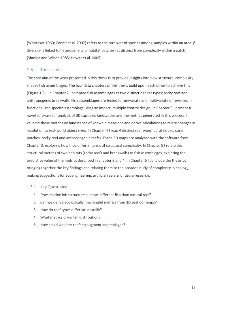
The core aim of the work presented in this thesis is to provide insights into how structural complexity 

shapes fish assemblages. The four data chapters of this thesis build upon each other to achieve this 

(Figure 1.3).  In Chapter 2 I compare fish assemblages at two distinct habitat types; rocky reef and 

anthropogenic breakwalls. Fish assemblages are tested for univariate and multivariate differences in 

functional and species assemblage using an impact, multiple control design. In Chapter 3 I present a 

novel software for analysis of 3D captured landscapes and the metrics generated in this process. I 

validate these metrics on landscapes of known dimensions and derive calculations to relate changes in 

resolution to real‐world object sizes. In Chapter 4 I map 4 distinct reef types (coral slopes, coral 

patches, rocky reef and anthropogenic reefs). These 3D maps are analysed with the software from 

Chapter 3, exploring how they differ in terms of structural complexity. In Chapter 5 I relate the 

structural metrics of two habitats (rocky reefs and breakwalls) to fish assemblages, exploring the 

predictive value of the metrics described in chapter 3 and 4. In Chapter 6 I conclude the thesis by 

bringing together the key findings and relating them to the broader study of complexity in ecology, 

making suggestions for ecoengineering, artificial reefs and future research.  

1.3.1  Key Questions: 

1. Does marine infrastructure support different fish than natural reef? 

2. Can we derive ecologically meaningful metrics from 3D seafloor maps? 

3. How do reef types differ structurally?  

4. What metrics drive fish distribution? 

5. How could we alter reefs to augment assemblages? 

 

 

 

14  

 

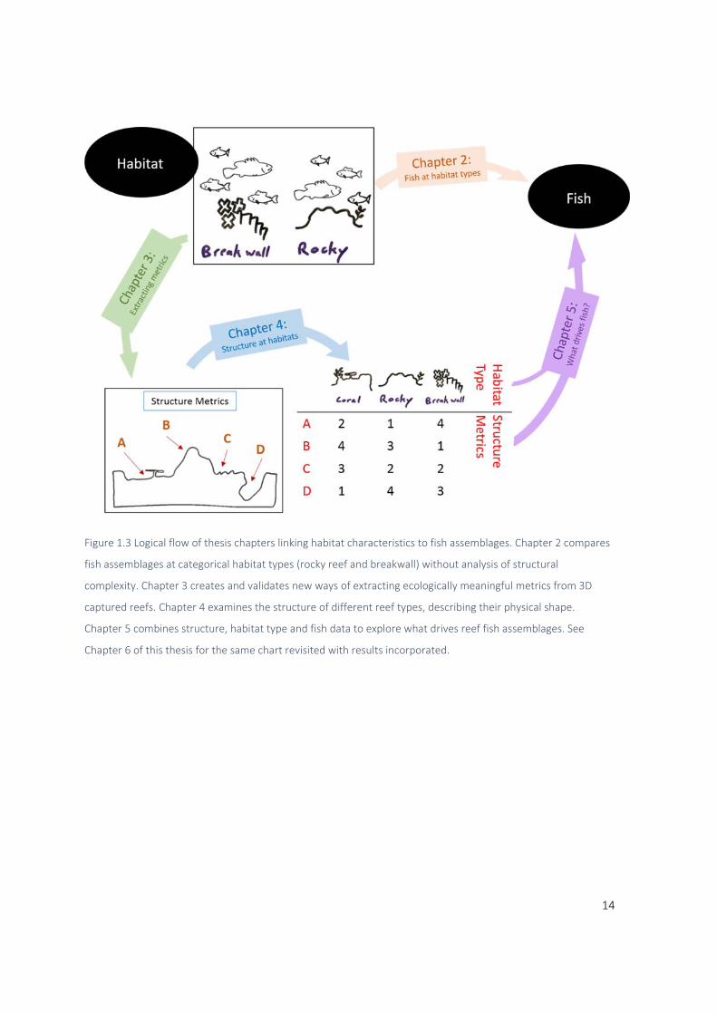
Figure 1.3 Logical flow of thesis chapters linking habitat characteristics to fish assemblages. Chapter 2 compares 

fish assemblages at categorical habitat types (rocky reef and breakwall) without analysis of structural 

complexity. Chapter 3 creates and validates new ways of extracting ecologically meaningful metrics from 3D 

captured reefs. Chapter 4 examines the structure of different reef types, describing their physical shape. 

Chapter 5 combines structure, habitat type and fish data to explore what drives reef fish assemblages. See 

Chapter 6 of this thesis for the same chart revisited with results incorporated. 

 

 

15  

Chapter 2: Marine infrastructure supports abundant, diverse fish 

assemblages at the expense of β diversity 

 

Summary 

1. Breakwalls support diverse, abundant and high‐biomass assemblages, often more so than 

natural reefs. 

2. Fish assemblages at 2 of 3 breakwalls differ from natural reef controls by having higher 

species richness and a greater abundance of mid‐water piscivores. 

3. Despite high transect‐scale diversity at breakwalls, landscape‐scale β diversity is sometimes 

low. 

2.1  Introduction 

The expanding global human population is intensifying environmental impacts, especially along 

coastlines (Burke et al. 2001; Duarte 2014).  Anthropogenic habitat manipulation is significant and 

increasing in marine ecosystems, with over half of shorelines altered by engineered structures in parts 

of Europe, North America, Australia and Asia (Dafforn et al. 2015). These changes to the physical 

structure of coastlines can have substantial impacts on local flora and fauna associated with the 

substratum (Clynick et al. 2008; Bulleri and Chapman 2010; Chapman and Underwood 2011; Dugan et 

al. 2011). Indeed, hardening shorelines with engineered structures can reduce ecosystem services 

(Gittman et al. 2016), fragment habitats (Bishop et al. 2017) and impact sessile and benthic organisms 

(Heery et al. 2017). We are also starting to develop a mechanistic understanding of the effects these 

changes have on mobile fish assemblages (Davis and Smith 2017; Morris et al. 2018). Recent work in 

the field of ecoengineering has identified promising developments in mitigating impacts to intertidal 

biodiversity (Browne and Chapman 2011), threatened species (Perkol‐Finkel et al. 2012), bivalves 

(Strain et al. 2017), ecosystem services (Mayer‐Pinto et al. 2017) and social values (Morris et al. 2016).  

But significant gaps remain in our knowledge about how mobile organisms, such as fish, relate to 

these structures (Morris et al. 2017). This information is required to predict impacts of future 

shoreline hardening and facilitate the development of effective mitigation measures.  

 

16  

Breakwalls, (aka. breakwaters) are an example of shoreline armouring commonly used around the 

world in shore stabilisation and the construction of marinas and canals.  Breakwalls provide habitat 

distinct from most natural reefs in terms of slope, habitat structural complexity and substratum 

material. There is sparse and sometimes conflicting information about how fish respond to breakwall 

habitats (Gittman et al. 2016). Diversity and species richness are often greater on breakwalls than 

adjacent natural reefs (Burchmore et al. 1985; Smith 1994; Stephens Jr et al. 1994; Burt et al. 2009; 

Burt et al. 2012; Fowler and Booth 2013). However, questions remain about the overall effects of 

breakwalls on fish assemblage structure with few studies examining this response and significant 

disagreement among them (Morris et al. 2017; Strain et al. 2018). Latitudinal gradients in diversity 

and abundance of fishes (Stuart‐Smith et al. 2013) leave open the possibility of interacting effects of 

habitat and latitude. However, even when comparing breakwalls of similar construction in the same 

region, some breakwalls support similar fish assemblages to natural reef, while others differ 

significantly (Burt et al. 2013).  

While many impacts are local (e.g. artificial reef or breakwall) fish assemblages are mobile and often 

quite variable (Smith et al. 2008). Capturing trends among this variation requires replication at scales 

that are often not feasible for ecological impact studies (Strain et al. 2018).  Additionally, fish 

responses to structural changes in their environment are not necessarily consistent across different 

spatial scales (Morris et al. 2017). Thus, studies encompassing scales from at least 10s to 100s of 

metres, and ideally including multiple controls, are needed to effectively examine the responses of 

mobile fish to anthropogenic impacts.  

It is clear that the physical shape and structure of a substratum influences the local fish assemblage 

(Nash et al. 2014; Ferrari et al. 2017). The number of species detected on artificial reefs is often much 

greater than on natural reefs (Branden et al. 1994; Hackradt et al. 2011). While patch size is likely 

contributing to these differences (Koeck et al. 2014), complexity is implicated as a primary cause 

(Perkol‐Finkel et al. 2006; Kovalenko et al. 2012; Pastor et al. 2013). Breakwalls are usually not 

designed with fish communities in mind, but they share many characteristics with artificial reefs that 

are designed for fish (Morris et al. 2018). Namely, they often have high vertical relief, are made of 

large concrete or rock objects, and have a large number of physical niches or holes. If assemblages of 

fish are influenced by the physical structure of the local substratum, then we would expect 

assemblages at breakwall habitat to differ from those at natural reef due to the different physical 

 

17  

shapes of the habitats. Likewise, the physically distinct shapes of breakwall habitat likely influence fish 

alpha diversity at these habitats. 

In addition to the species that constitute local assemblages, it is important to know whether breakwall 

habitat emulates the ecological functions of natural reefs. Grouping organisms by functional traits can 

give an indication of the ecological function of a habitat (Bremner et al. 2006; Stuart‐Smith et al. 

2013). Increases in the number of functional groups present is understood to improve ecosystem 

function (Tilman 2000) and functional traits have been used as a surrogate for ecosystem health 

(Hewitt et al. 2008b). Likewise, if functional groups (e.g. herbivores) are missing from a habitat, this is 

likely to reduce ecological function. There is evidence that anthropogenic habitats often do not 

support assemblages fulfilling the same ecological function as their natural counterparts (Strain et al. 

2018). The number of ecological niches being exploited (functional richness) on purpose‐built artificial 

reefs has been shown to be higher than natural reefs (Koeck et al. 2014). However, marine 

infrastructure (e.g. pilings) has been shown to support assemblages of fish that are functionally poor 

compared to natural reefs (Rilov and Benayahu 1998). It is possible that the increased complexity, 

niches, and proximity to other habitat types of breakwall habitat will support greater functional 

richness than natural reefs, but this has not yet been robustly tested. It is also possible that, like other 

infrastructure, breakwalls support assemblages which are performing relatively few ecological 

functions. Therefore, examining the functional roles being performed by assemblages at breakwall 

habitat is important. 

Another potentially important way in which shoreline armouring differs from natural reefs is in its 

homogeneity. While different armouring structures vary in their surface roughness, each one is 

typically built with consistent materials throughout. This is analogous to low landscape heterogeneity 

and is likely to have important ecological implications for local assemblages of fish (Ellingsen 2002). β ‐

diversity (the turnover of species among samples within a larger area) (Whittaker 1960; Condit et al. 

2002) is one aspect of an assemblage that is known to respond to landscape heterogeneity (Shmida 

and Wilson 1985; Hewitt et al. 2005). Marine rocky reefs remain heterogeneous at scales of 10s of 

metres (transect‐scale in this study) through 100s of metres (landscape‐scale in this study) (Connell 

and Irving 2008). Engineered structures such as breakwalls also provide heterogeneous habitat at the 

scale of 10s of meters, with large overhangs, cracks and crevices and this is likely driving the high 

alpha diversity at these habitats. However, at the scale of 100s of metres, breakwalls have low 

heterogeneity as they typically employ a uniform design across the whole structure. This landscape‐

 

18  

scale uniformity is likely to result in low β ‐diversity as the assemblages at each transect are relatively 

similar to each other due to almost identical underlying habitats (Hewitt et al. 2005). However, to our 

knowledge, β ‐diversity of mobile organisms has not been studied on breakwalls. 

In this study we quantify fish assemblages at natural reefs and breakwalls in order to evaluate 

hypotheses about fish use of marine infrastructure. Assemblages are grouped by species identity, and 

by functional groups. Each hypothesis applies to both grouping methods. We predict that: 

1. Abundance and biomass will be greater at breakwall habitat.  

2. Richness (α diversity) will be greater at breakwall habitat.  

3. Landscape‐scale β diversity will be lower at breakwall habitat. 

4. Assemblage structure will differ between natural and breakwall habitat.  

2.2  Methods 

2.2.1  Study area and design 

Fish assemblages were surveyed on breakwalls and natural reefs at three regions spanning 531 

kilometres across a sub‐tropical – temperate transition zone along the SE coast of Australia; Coffs 

Harbour (CH) (30°18'13.42"S, 153° 8'52.23"E), Botany Bay (BB) (33°58'56.81, 151°12'52.32"E) and Port 

Kembla (PK) (34°27'46.43"S, 150°54'20.84"E) (Figure 2.1). All sites consisted of rocky reefs supporting 

interspersed kelp and sand patches.  The design was asymmetrical at the level of site because 

comparable breakwalls are limited in size, number and geographical distribution. Thus, at each region 

there was one site for the breakwall reef type and three sites for the natural reef. Six replicate 

transects were sampled at each site.  

 

19  

 

Figure 2.1 Map of study sites. Three regions (Coffs Harbour, Botany Bay, Port Kembla), each with one breakwall 

(red) and three natural reef controls (black). 

 

Each region had a breakwall site that was selected to minimize differences in confounding 

environmental variables (i.e. exposure, aspect, depth, adjacent habitat types) that could influence fish 

assemblages. The breakwalls at CH and PK protect coastal marinas and the BB breakwall bordered a 

cargo area for commercial shipping ~2.5 km inside a large open bay with limited estuarine input, but 

dominated by oceanic water (Jones and Candy 1981). At each breakwall site, the oceanic side of the 

wall was sampled. All breakwalls were constructed from a mix of concrete coastal protection 

structures known as tetrapods (Gürer et al. 2005), concrete blocks (~1.5m3) and/or large boulders. All 

breakwalls were older than 40 years.  

 

20  

Within each region, 3 natural reefs (control sites) were selected to minimize environmental 

differences among them and the breakwall site (i.e. pollutants, depth, exposure, reef size, general 

habitat condition). All sites supported benthic assemblages that were characteristic of the naturally 

variable healthy reefs in the region (kelp, branching algae, turfing algae, occasional coral at CH and 

sparse kelp and branching algae, cunjevoi, bare rock and encrusting algae at BB and PK). All reefs were 

between 420 and 1800 m in length with a mean length of 1260 m. Breakwall lengths were 660 m at 

CH, 1720 m at BB and 1240 m at PK. Photos of representative reef patches were taken at each site 

(Figure 2.2). Mean distance from natural reefs to their respective breakwall was 4.8 ± 2.1 SE km (<1% 

of the total study area) ensuring that the sites were exposed to similar temperature and 

oceanographic conditions. Sites were chosen to balance proximity to breakwalls with comparability of 

habitat (i.e. aspect, patch size, depth) and all sites in a region were sampled in the same season. All 

transects (breakwall and natural reef) were evaluated at places sheltered from the prevailing 

southerly swell, over hard substrata (concrete /boulders at breakwalls, solid rock/boulders at natural 

reef) and bordered by open sand flats. All transects were between 2 and 10 m deep with mean depths 

for a site ranging from 4.2 (CH 1) to 7.5 (PK 4). All of the transects were in areas where fishing is 

permitted. All field work was conducted in 2015: PK was sampled in May, CH was sampled in July – 

Sept, and BB was sampled in Oct – Nov. 

 

 

21  

 

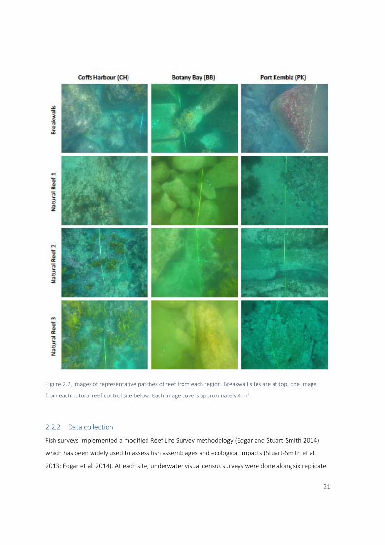
Figure 2.2. Images of representative patches of reef from each region. Breakwall sites are at top, one image 

from each natural reef control site below. Each image covers approximately 4 m2. 

 

2.2.2  Data collection 

Fish surveys implemented a modified Reef Life Survey methodology (Edgar and Stuart‐Smith 2014) 

which has been widely used to assess fish assemblages and ecological impacts (Stuart‐Smith et al. 

2013; Edgar et al. 2014). At each site, underwater visual census surveys were done along six replicate 

 

22  

25 x 10 m transects demarcated using tape measures prior to the survey. Each transect was at least 10 

m from others to ensure independence of samples. Fish were visually sampled by two divers 

experienced in conducting visual censuses of fish on SCUBA. Divers were randomly allocated sites to 

minimise systematic biases associated with any one sampler. Divers sampled transects in pairs, and 

each diver sampled a longitudinal half of each transect (5 m on one side of the transect tape and 5 m 

off the substratum). Fish were identified to species level, counted and sized into length classes of 2.5, 

5, 7.5, 10, 20, 35, 50+ cm. Counts from the two divers were summed to produce a total count for each 

250 m2 transect. Searches for cryptic species (Reef Life Survey method 2) were not conducted. Highly 

mobile coastal pelagic species (e.g. Yellowtail Scad Trachurus novaezelandiae and Common Jack Mackerel T. 

declivis) were excluded from the study. These mobile schooling species were extremely patchy (98% of 

them encountered at one breakwall and one natural reef site) and not well quantified at the scale of 

this study. 

2.2.3  Fish Groups 

Fish data were aggregated, and total abundance and biomass were calculated for each site. All fish 

were subsequently grouped in two ways: A ‐ assemblage grouped by species identity; B ‐ assemblage 

grouped by functional groups. Both of these expressions of the observed assemblage were analysed 

for the following metrics:  

1. Richness (α diversity) 

2. β diversity 

3. Multivariate assemblage structure 

Species were categorized into one of 15 functional groups based on the combination of their water 

column position (3 categories) and their trophic level (5 categories) (see Appendix 1 for full list of 

species and functional groups).  The three levels of water column position were: mid‐water, demersal 

(associated with, but not living in the benthos), and benthic (living in/on the benthos). The five trophic 

groups were: planktivores, herbivores, infauna predators (feeding primarily on organisms in/on the 

benthos), meso‐predators (feeding on a range of small organisms with opportunistic piscivory) and 

piscivores. This combination of trophic niche and positional niche is designed to capture the most 

ecologically important functions on a reef, while not splitting the assemblage into categories so small 

they are not reliably detected. This approach is known to be sensitive to changes in habitat (Ferrari et 

al. 2017). Functional groups were identified using information from Fishbase.org and dietary 

 

23  

information from field guide (Kuiter 1993). Fifteen individual cleaner wrasses from 2 species were 

excluded from this analysis as it was deemed they did not warrant the inclusion of a separate 

“cleaner” trophic category. 

2.2.4  Univariate metrics    

Four univariate metrics (total abundance, total biomass, richness, β diversity) were calculated for each 

transect. Total abundance was the number of individual fish detected in a transect. Biomass was 

calculated for individual fish based on established length‐weight relationships for each species (Duffy 

et al. 2016).  While α diversity (richness) captures the diversity within a transect, β diversity quantifies 

the variability (percent unshared species) among transects at a site.  Jaccard’s index of β diversity was 

calculated using Bray‐Curtis dissimilarity matrices on presence/absence transformed abundance data 

(Jaccard 1900b; Anderson 2006). This metric gives an indication of the species differences among 

transects within a site. Where transects share a high proportion of species (low species turnover) β 

diversity is low, irrespective of diversity at each transect. All univariate responses except β diversity 

used Euclidian distances to generate similarity matrices for statistical tests. 

2.2.5  Statistical analysis  

Species abundance data were log transformed to reduce the influence of a few abundant species 

(Clarke 1993). Functional groups were presence/absence transformed to test if assemblages filled a 

similar numbers of functional niches at different habitats. Both abundance and functional group data 

used Bray‐Curtis similarity matrices (Bray and Curtis 1957) for the tests described below. Differences 

among assemblages were visualized using a non‐metric multi‐dimensional scaling plot (nMDS) (Field 

et al. 1982). Dispersion of assemblages was tested using PERMDISP (Anderson 2006). Individual 

species and functional groups were then ranked according to their contribution to assemblage 

differences between the two reef types using similarity percentage (SIMPER) analysis (Clarke and 

Gorley 2006). All multivariate analyses were performed using routines in the PRIMER6 + PERMANOVA 

package. 

We used the same analysis structure for all response variables. Permutational Analysis of Variance 

(PERMANOVA) (Anderson et al. 2008) was used to test for main and interactive effects of the factors 

site, reef type and region in both univariate and multivariate response variables. Permutation‐based 

analyses have been shown to be effective for univariate tests (Anderson and Millar 2004) and robust 

to the non‐normality often experienced in variable marine community data (Anderson 2001; Kelaher 

 

24  

and Castilla 2005). We used 9999 permutation (residuals under reduced model) with type 3 (partial) 

sums of squares. Where few unique permutations were possible, Monte Carlo p‐values are presented. 

Where interactions involving region were detected, data from each region were analysed separately. 

PERMDISP analyses were used to test for differences in dispersion among sites in a region (Anderson 

and Walsh 2013). At each region, an asymmetrical design was utilised with 1 breakwall site and 3 

natural reef sites. The fixed factor reef type had 2 levels (breakwall and natural reef), site (random) 

was nested within reef type (1 site on breakwall and 3 sites on natural reef), and each site had 6 

replicate transects. This model compared breakwall assemblages to those on natural reefs with an 

estimate of variability among natural reef sites in a region. Due to the inherent variability of 

assemblages among natural reefs and the partitioning of variability for nested factors, this model is 

likely to be conservative at the level of reef type (Underwood 1994). This design provides a robust test 

of differences among control and impacted sites (Underwood 1991). 

2.3  Results 

At the 72 transects conducted for this study, 34,157 reef‐associated fishes were detected from 112 

species and 12 functional groups (Appendix 1). There was a consistent interaction between region and 

reef type, whereby CH showed different patterns than BB and PK. 

2.3.1  Univariate metrics    

The full models indicated significant interactions between region and reef type (Appendix 2). 

Therefore, regions were analysed separately to test hypotheses about differences between habitat 

types at each region.  There were no differences in the metrics for CH but in the other two regions 

univariate metrics differed significantly (Figure 2.3). In these two regions, the average breakwall 

transect had 784 more individual fish, 8 more species and 33% greater diversity, which translated to 

634% more biomass than adjacent natural reef transects.  Of the seven univariate metrics tested 

(abundance, biomass, species richness, diversity, functional richness and β diversity) only functional β 

diversity showed a consistent pattern, remaining equal at all three breakwall/natural reef contrasts 

(Appendix 3). The only metric that was significantly greater on natural reef habitat was β diversity at 

PK. 

 

 

25  

 

Figure 2.3. Univariate metrics (Abundance, Biomass, Species Richness, Functional Richness, β Diversity, and 

Functional β Diversity) on contrasting reef types (breakwall = black, natural reef = white) at each region. 

Asterisks indicate significant difference (p < 0.05) between breakwall and all control reefs in that region. 

 

26  

2.3.2  Multivariate metrics    

2.3.2A  Assemblage Grouped by species 

Assemblage data grouped by species showed a significant interaction between region and reef type 

(Pseudo‐Fx,y = 5.0615 , Pperm = 0.0001), indicating that differences in multivariate assemblages 

between breakwall and natural reef were not consistent across regions. Each region, therefore, was 

analysed independently.  

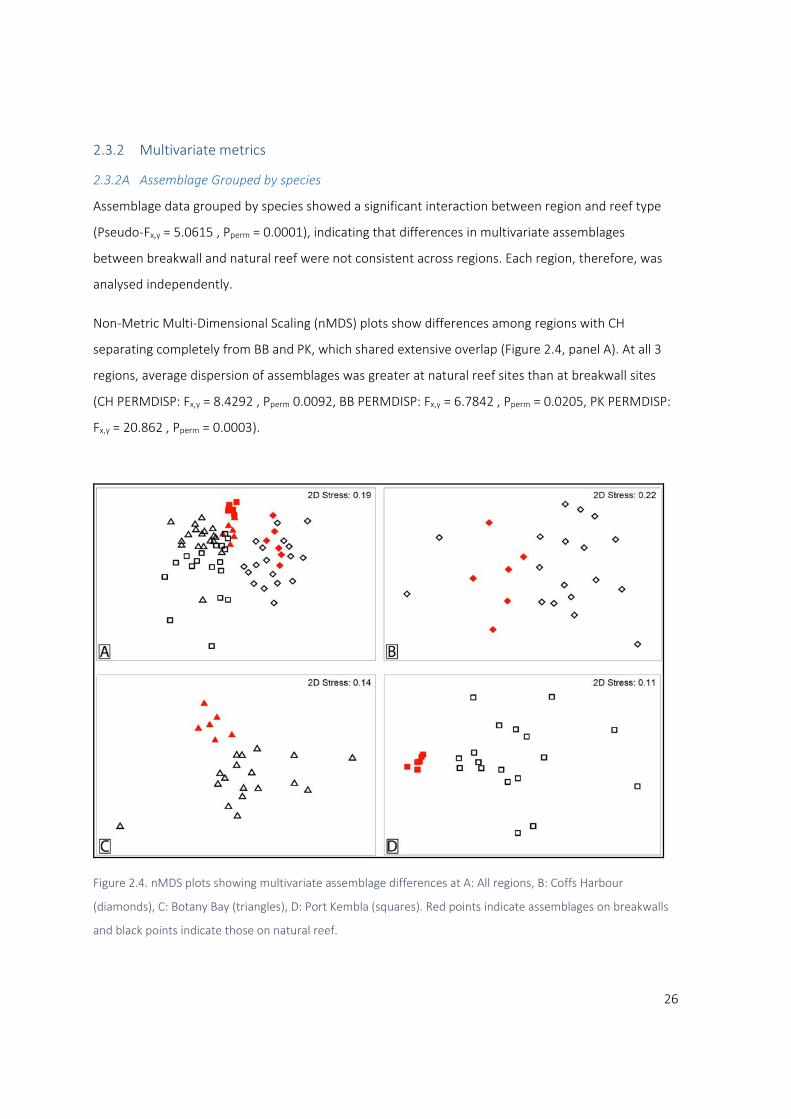
Non‐Metric Multi‐Dimensional Scaling (nMDS) plots show differences among regions with CH 

separating completely from BB and PK, which shared extensive overlap (Figure 2.4, panel A). At all 3 

regions, average dispersion of assemblages was greater at natural reef sites than at breakwall sites 

(CH PERMDISP: Fx,y = 8.4292 , Pperm 0.0092, BB PERMDISP: Fx,y = 6.7842 , Pperm = 0.0205, PK PERMDISP: 

Fx,y = 20.862 , Pperm = 0.0003).  

 

 

Figure 2.4. nMDS plots showing multivariate assemblage differences at A: All regions, B: Coffs Harbour 

(diamonds), C: Botany Bay (triangles), D: Port Kembla (squares). Red points indicate assemblages on breakwalls 

and black points indicate those on natural reef. 

 

27  

Asymmetrical analysis of variance at CH confirmed similarities in assemblages on different reef types 

(Pseudo‐Fx,y = 1.2876  , Pmc = 0.2969). At BB, variability among natural reefs outweighed the differences 

between reef types resulting in a non‐significant asymmetrical PERMANOVA (Pseudo‐Fx,y = 2.031 , Pmc 

= 0.1328, Appendix 4). This result remained even when the outlier transect visible in the bottom left 

of Figure 2.4C was removed.  Assemblage structure differed between reef types at PK (Pseudo‐Fx,y = 

3.0941 , Pmc = 0.0449). 

SIMPER analysis revealed that Mado (Atypichthys strigatus) and Eastern Pomfred (Schuettea 

scalaripinnis) were among the top three contributors to differences between breakwall and natural 

reef assemblages in all regions. Mado contributed between 6.8% and 9.9% and Pomfred contributed 

between 5.7% and 9.82% (see Appendix 5 for Simper results). Mado were consistently more abundant 

on breakwall habitat across all regions. Pomfred, however, showed a strikingly different pattern across 

regions. At CH, Pomfred were abundant on natural reef habitat, and completely absent from 

breakwall habitat. At BB and PK, the opposite was the case with Pomfred abundant on breakwall 

habitats and rare or absent from natural reefs. The planktivore Silver Sweep (Scorpis lineolata) was 

consistently more abundant on breakwall habitat and was among the top six contributors to 

assemblage differences at all regions (4.03% at CH, 8.59% at BB and 5.49% at PK). 

2.3.2B  Assemblage Grouped by functional traits 

Of the 15 functional groups based on the combination of traits, 12 were detected in this study. 

Planktivores accounted for 11.6% of the individual fish detected, herbivores 18.8%, infauna predators 

13.4%, meso‐predators 45.5% and piscivores 10.7%. In terms of water‐column position, 79.5% were 

demersal, 7.1% were mid water column and 13.4% were benthic. 

Differences in multivariate assemblages between breakwall and natural reef were not consistent 

across regions in that analyses of assemblage data grouped by functional groups showed significant 

interactions between region and reef type (Pseudo‐Fx,y = 4.5558 , Pperm 0.0002, Appendix 6). 

Dispersion of functional group assemblages was not significantly different between breakwall and 

natural reef habitat in any of the regions (CH Fx,y = 1.3919, Pperm = 0.3195, BB Fx,y = 0.1877, Pperm = 

0.7009, PK Fx,y = 4.5836, Pperm = 0.0597). Removing the natural reef outlier at PK (see Figure 2.5D) did 

not change this result. Overall functional assemblages were not significantly different between 

breakwall and natural reef habitats in any of the regions (Figure 2.5, Appendix 7) (CH, Pseudo‐Fx,y = 

0.6226, Pmc = 0.6192, BB, Pseudo‐Fx,y = 0.7170, Pmc = 0.5571, PK, Pseudo‐Fx,y = 1.3996, Pmc = 0.3433). 

 

28  

 

 

Figure 2.5. nMDS of fish assemblages aggregated to by functional group at A: All regions, B: Coffs Harbour 

(diamonds), C: Botany Bay (triangles), D: Port Kembla (squares).  Red points indicate assemblages on breakwalls 

and black points indicate those on natural reef. Where multiple points have mapped onto the same location, 

they appear as red with a black outline. 

 

SIMPER analyses indicated underlying trends in distribution of these functional groups. As with other 

measures, there was a strong interaction between regions and reef type with CH showing different 

patterns than BB and PK. At CH, benthic and demersal predator categories were more abundant on 

breakwall reefs (contributing 13%–15% to differences, see Appendix 8), while demersal planktivores 

and midwater piscivores were more abundant at natural reefs, contributing 21% and 12% 

respectively. At both PK and BB, however, mid‐water piscivores (primarily Long‐fin Pike (Dinolestes 

lewini) and Snapper (Chrysophrys auratus)) were more abundant at breakwall reefs and contributed 

strongly (23% at PK and 21% at BB) to breakwall/natural reef assemblage difference.  

 

29  

2.4  Discussion 

This study found that fish assemblage metrics showed mixed results across the three regions. Species 

richness was significantly greater at breakwall habitat than natural reefs at two of the three regions 

studied. Hypotheses about abundance and biomass were not supported, with each being greater in 

breakwall habitats at only 1 of 3 regions (Table 2.1). Hypotheses about species α diversity being 

greater in breakwall habitats were supported at BB and PK with Luderick (Girella tricuspidata), 

Yellowfin Bream (Acanthopagrus australis) and Eastern Pomfred (S. scalaripinnis) among other species 

frequently found at breakwalls, but not natural reefs.  Hypotheses about functional α diversity, 

species β‐diversity and assemblage structure grouped by species were not supported, with each only 

being confirmed at 1 of 3 regions. Hypotheses about functional β‐diversity and assemblage structure 

grouped by functional traits were not supported at any region. 

Table 2.1. Level of support for hypotheses that univariate responses will be at each region. “+” indicates a 

significant (p < 0.05) result in the direction hypothesized, blank indicates insignificant result. There were no 

significant results opposite the direction hypothesized. 

  Species Identity Functional Groups

 Hypothesis  CH  BB PK CH BB PK

Total Abundance (BW > NR)   + +Biomass (BW > NR)    + +Richness (α Diversity) (BW > NR)    + + +β Diversity (BW < NR)    +Multivariate assemblage (BW ≠ NR)    +

 

When multivariate assemblages were grouped by species identity there were significant region x 

habitat interactions: this was the same for univariate metrics. Assemblages associated with the two 

habitats did not differ significantly at CH and BB, while they were distinct at PK, with Mado (A. 

strigatus) and Eastern Pomfred (S. scalaripinnis) more abundant at breakwalls. These conflicting 

results are consistent with previous studies on the effect of breakwalls on fish assemblages (Pérez‐

Ruzafa et al. 2006; Burt et al. 2009; Burt et al. 2013; Fowler and Booth 2013; Taira et al. 2017). There 

have been two previous studies of fish at breakwall and natural reef habitat at the same bay as BB in 

this study (Burchmore et al. 1985; Fowler and Booth 2013). Though they sampled different areas of 

breakwall and each only used one natural reef control. Both studies found increased richness and 

abundance at breakwall habitat, but findings on multivariate assemblage structure disagreed with 

Burchmore et al. (1985) reporting a significant difference while Fowler and Booth (2013) found no 

difference. In the case of Fowler and Booth, the breakwall had 30+ years to establish a mature benthic 

 

30  

community. In the case of Burchmore et al., however, the breakwall community only had 8‐10 years 

to establish which is marginal for considering a community to be mature (Perkol‐Finkel and Benayahu 

2005). It is possible that resulting differences in benthic assemblage were driving the differences 

between assemblages at the two habitat types. Conversely, these findings may simply highlight the 

inherently variable nature of these habitats over space and time (Stephens Jr et al. 1994; Fowler and 

Booth 2013).  

2.4.1  Functional groups 

Hypotheses about multivariate assemblages grouped by functional traits were not supported with no 

significant differences detected. These results indicate that even when species identity and 

abundance of assemblages differed among sites, similar functional niches were filled.  

Hypotheses about functional richness were not supported at two of the three regions. Functional 

richness was not significantly different between natural reefs and breakwalls at CH or PK. These 

findings suggest that breakwall habitat is functioning similarly to surrounding natural reefs. Breakwall 

habitat at BB, however, had significantly higher functional richness as well as elevated species 

richness. This suggests that some of the additional species present at the BB breakwall were from 

functional groups not found at the natural reefs. Investigating these trends further with SIMPER 

analyses highlighted the higher prevalence of midwater piscivores on the breakwall at BB. Specifically, 

higher prevalence of Long‐fin Pike (D. lewini) and Snapper (C. auratus) were primarily responsible for 

these differences. Both of these fish are important fisheries species in NSW (Griffiths 2012). 

Additionally the presence of larger, higher‐trophic‐order species like piscivores is consistent with 

relatively un‐impacted ecosystems (Duffy 2003). These findings would suggest that the breakwall 

habitats studied here are functioning similarly to surrounding natural reefs. 

2.4.2  Trophic structure 

While the high occurrence of midwater piscivores on breakwalls at PK and BB is a desirable 

recreational fishing outcome, it also raises questions about the ecological function of this habitat. 

Similar patterns have been documented at other breakwalls (Burt et al. 2009) and attributed to 

availability of small prey fishes. The idea of an ecological trap (Dwernychuk and Boag 1972), or 

attractive sink (Pulliam 1988; Doak 1995) is that individuals can be drawn to an area that is ultimately 

detrimental to their survival or fitness. This idea has been applied to artificial reefs (Grossman et al. 

1997) because they concentrate fish in small areas, subjecting them to high fishing pressure. While 

 

31  

this is a hotly contested debate in the artificial reef literature (Brickhill et al. 2005), the idea that fish 

could be attracted from natural reef to breakwall habitat, only to suffer exceptionally high mortality 

from fishing warrants consideration. This idea is predicated on there being high fishing pressure at 

breakwalls. However, we were unable to find any studies quantifying this. If breakwalls were indeed 

acting as an ecological trap, drawing  fish to a habitat where they experience exceptionally high fishing 

pressure, we would expect to find size spectra skewed towards small individuals (Dulvy et al. 2004). 

This trend was not observed, with high numbers of both large and small individuals found at 

breakwalls. At all regions, fish in the 10 cm and 20 cm length categories accounted for the most 

biomass (Appendix 9). The breakwalls at BB and PK supported elevated biomass overall, including 

from large individuals (35‐cm category). The data on small individuals (5 cm and 7.5 cm classes) 

presents a mixed picture. At the BB breakwall levels of small individuals fall in line with natural reefs. 

At PK, however, breakwall habitat supported high biomass of small individuals. These data are 

certainly not enough to rule out the ecological trap model, but neither do they support it. 

2.4.3  Regional differences 

This study consisted of 3 comparisons between breakwall habitat and natural reef controls in the local 

area. By necessity it spanned a latitudinal gradient. The three regions in this study are exposed to 

different levels of environmental stressors. PK has high levels of metal contamination and BB is 

recovering from historical metals pollution (Piola and Johnston 2006). Commercial boat traffic at BB 

and PK is also likely to be higher than CH, as they are active commercial ports. It is unknown if these 

factors influence the local fish assemblages but unlikely that they are driving differences between 

habitat types as all sites in a region are exposed to similar levels of these stressors. 

While latitudinal gradients were not the focus of this study, some patterns emerged. One strong 

pattern is the region x habitat interaction whereby breakwall habitat affected fish at BB and PK, but 

not at CH. The strongest pattern was increased diversity and richness at breakwall habitat in BB and 

PK. This begs the question why fish assemblages did not differ between breakwall and natural reef 

habitat at CH. The habitat heterogeneity model (Tews et al. 2004) states that more heterogeneous 

habitats support more diverse assemblages. The natural reefs at CH are notable for supporting 

patches of dense macro algae over rocky reef, as well as interspersed coral habitat (Harriott et al. 

1994; Malcolm et al. 2010). In contrast, the natural reefs at both BB and PK were exclusively rock with 

some macro algae. Following the habitat heterogeneity model, this would suggest that the similarity 

between assemblages at breakwall and natural reef habitat at CH is driven by elevated diversity at 

 

32  

natural reefs due to their high habitat heterogeneity. Indeed, the broader CH region is valued for its 

high biodiversity (Malcolm et al. 2010). It seems likely that observed differences between breakwall 

and natural reef habitat are moderated by the type of natural reef habitat adjacent to a breakwall. 

This likely contributes to the persistent discrepancies in studies comparing these habitat types. 

2.4.4  β diversity 

The physical structure of habitats is known to affect fish at different spatial scales (Nash et al. 2013). 

While transect‐scale richness and diversity were high at breakwall habitats, landscape‐scale β‐diversity 

showed a very different pattern. β‐diversity was consistently low at breakwall habitats, and this trend 

was significant at PK. In the context of the habitat heterogeneity model, it is important to note that 

landscapes can have different levels of structural heterogeneity at different scales. While the 

structural heterogeneity of natural environments tends to scale consistently (Mandelbrot and Pignoni 

1983), artificial reefs do not (Abelson and Shlesinger 2002). Therefore, it is not inconsistent to 

hypothesize that while the transect‐scale (10s of m) structural heterogeneity of breakwalls is high, the 

landscape‐scale (100s of m) structural heterogeneity could be low. Indeed, this is what would be 

expected of an engineered environment built of large complex objects (boulders, cement blocks, 

tetrapods) but constructed with the same material and design across the whole structure. While β 

diversity of mobile organisms on breakwall habitat has not been studied to our knowledge, habitats 

with low, large‐scale complexity have been shown to support less β‐diverse assemblages (Schneider et 

al. 1987; Hewitt et al. 2005) and studies have found similar patterns with sessile organisms on 

breakwalls (Aguilera et al. 2014). Therefore, it seems likely that the landscape‐scale uniformity of 

breakwall habitat is driving low β‐diversity, despite the high complexity and diversity at smaller scales. 

This broad‐scale uniformity has negative implications for diversity at regional (Ellingsen 2002) and 

global scales (Thomas 1990). Because β diversity measures the percent of unshared species between 

patches, it is sensitive to rare species. If detecting rare species was more difficult at one habitat type, 

this could have influenced the results. BW habitat tended to have more caves and overhangs, but 

dives were not timed, and these features were explored.  

This study tested categorical habitat types. But the variability of natural reefs is evident both visually 

(Figure 2) and in the fish assemblages (Figures 3, 4 and 5). Rigorously quantifying complexity (Matias 

et al. 2007; Figueira et al. 2015) as well as benthic assemblage would likely shed light on the drivers of 

the observed differences. Breakwalls are known to have increased slope, higher structural complexity, 

and more niches than most natural rocky reefs (Fowler and Booth 2013). This, coupled with the 

 

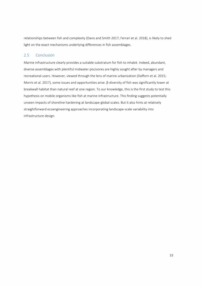
33  

relationships between fish and complexity (Davis and Smith 2017; Ferrari et al. 2018), is likely to shed 

light on the exact mechanisms underlying differences in fish assemblages.  

2.5  Conclusion 

Marine infrastructure clearly provides a suitable substratum for fish to inhabit. Indeed, abundant, 

diverse assemblages with plentiful midwater piscivores are highly sought after by managers and 

recreational users. However, viewed through the lens of marine urbanization (Dafforn et al. 2015; 

Morris et al. 2017), some issues and opportunities arise. β‐diversity of fish was significantly lower at 

breakwall habitat than natural reef at one region. To our knowledge, this is the first study to test this 

hypothesis on mobile organisms like fish at marine infrastructure. This finding suggests potentially 

unseen impacts of shoreline hardening at landscape‐global scales. But it also hints at relatively 

straightforward ecoengineering approaches incorporating landscape‐scale variability into 

infrastructure design. 

 

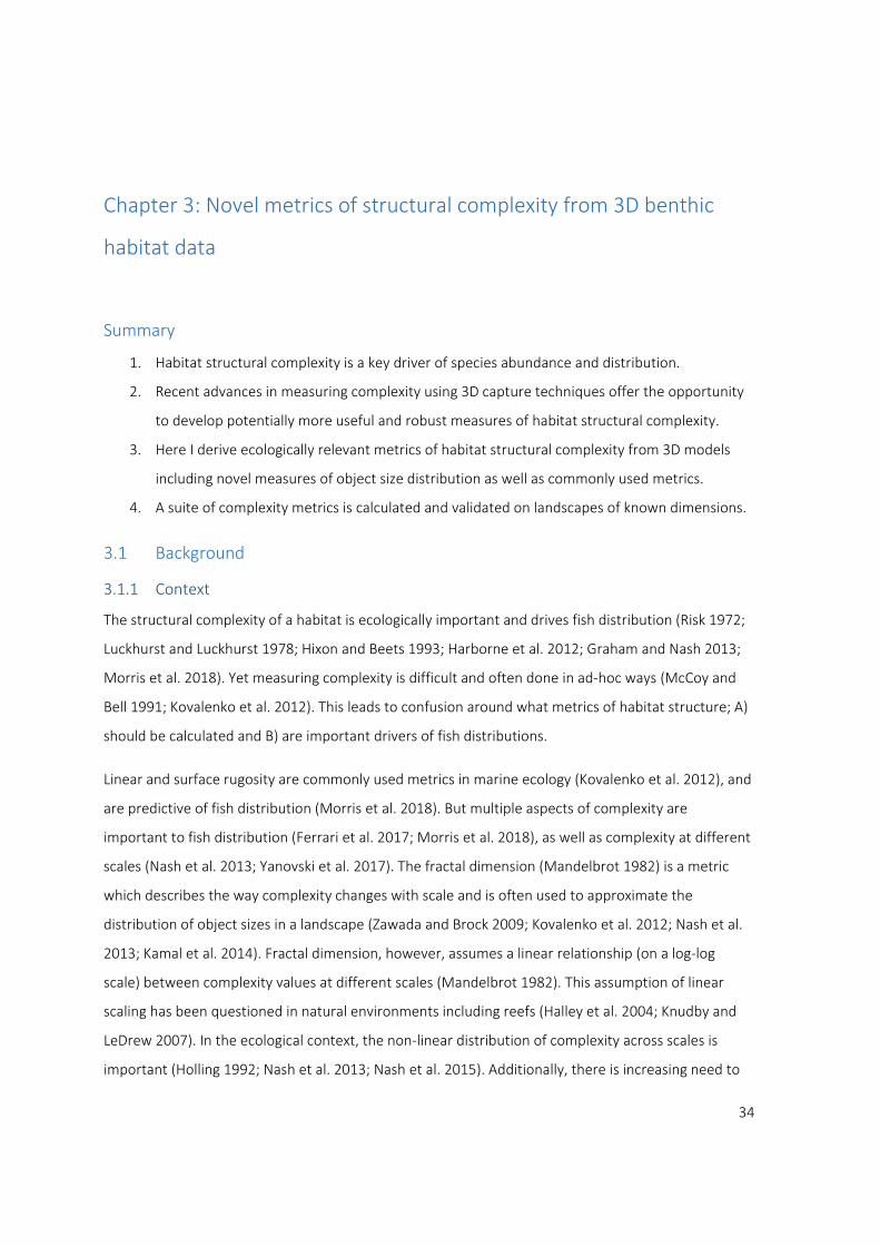
34  

Chapter 3: Novel metrics of structural complexity from 3D benthic 

habitat data 

 

Summary 

1. Habitat structural complexity is a key driver of species abundance and distribution.  

2. Recent advances in measuring complexity using 3D capture techniques offer the opportunity 

to develop potentially more useful and robust measures of habitat structural complexity. 

3. Here I derive ecologically relevant metrics of habitat structural complexity from 3D models 

including novel measures of object size distribution as well as commonly used metrics. 

4. A suite of complexity metrics is calculated and validated on landscapes of known dimensions. 

3.1  Background 

3.1.1  Context 

The structural complexity of a habitat is ecologically important and drives fish distribution (Risk 1972; 

Luckhurst and Luckhurst 1978; Hixon and Beets 1993; Harborne et al. 2012; Graham and Nash 2013; 

Morris et al. 2018). Yet measuring complexity is difficult and often done in ad‐hoc ways (McCoy and 

Bell 1991; Kovalenko et al. 2012). This leads to confusion around what metrics of habitat structure; A) 

should be calculated and B) are important drivers of fish distributions. 

Linear and surface rugosity are commonly used metrics in marine ecology (Kovalenko et al. 2012), and 

are predictive of fish distribution (Morris et al. 2018). But multiple aspects of complexity are 

important to fish distribution (Ferrari et al. 2017; Morris et al. 2018), as well as complexity at different 

scales (Nash et al. 2013; Yanovski et al. 2017). The fractal dimension (Mandelbrot 1982) is a metric 

which describes the way complexity changes with scale and is often used to approximate the 

distribution of object sizes in a landscape (Zawada and Brock 2009; Kovalenko et al. 2012; Nash et al. 

2013; Kamal et al. 2014). Fractal dimension, however, assumes a linear relationship (on a log‐log 

scale) between complexity values at different scales (Mandelbrot 1982). This assumption of linear 

scaling has been questioned in natural environments including reefs (Halley et al. 2004; Knudby and 

LeDrew 2007). In the ecological context, the non‐linear distribution of complexity across scales is 

important (Holling 1992; Nash et al. 2013; Nash et al. 2015). Additionally, there is increasing need to 

 

35  

develop design criteria for reefs that support abundant and diverse assemblages of fish (Morris et al. 

2016; Mayer‐Pinto et al. 2017; Morris et al. 2018). Rugosity, while useful as a predictor of fish 

distribution, is not useful as a design criterion as it provides very little explicit information about the 

nature of the structure itself (e.g, size, volume…).  

In this chapter I develop standardized analysis of 3D data across different scales and introduce a new, 

structurally explicit way of analysing object sizes in a landscape. Algorithms for metric extraction have 

been included in a software package for repeatability (see Chapter 3 Appendices). 

3.1.2  3D data 

3D data is a collection of triangular faces positioned in space to model a surface. True 3D data is 

different from most structural data that is commonly referred to as “3D” (eg. raster or height field 

data) in that it can capture surfaces beyond vertical. For ecological applications this distinction is 

highly important as overhangs and downward‐facing surfaces are ecologically distinct (Connell 2001; 

Clynick et al. 2007). In this thesis I use structural data collected with the methods outlined in Figueira 

et al. (2015). Therefore, I use the term 3D as distinct from 2.5D (which would apply to raster or height 

field data) to indicate data that includes surfaces beyond vertical. The data presented in this chapter 

are triangulated irregular networks (TINs) (Peucker et al. 1978) captured using underwater 

photogrammetry following Figueira et al. (2015). 

The field of remote sensing shares many questions about structure with fish ecologists working at 

smaller scales. As such there are existing approaches, metrics and packages to extract data from 

satellite derived imagery using Geographical Information Systems. Some of these approaches have 

been used in conjunction with photogrammetry for ecological questions (Friedman et al. 2012; Burns 

et al. 2015). These metrics, however, typically are not built for true 3D data as they were often 

developed with raster data structures in mind. 

3.1.3  Metrics of complexity 

There is no unified suite of metrics extracted from 3D models, or even a standardized method for 

attaining these structural complexity data (Loke et al. 2015). Several metrics are commonly calculated 

and appear to be useful in understanding fish distribution. Slope, vertical relief, surface orientation 

and rugosity are all ecologically important metrics (Kovalenko et al. 2012; Morris et al. 2018). In 

addition to the above metrics, the size of features in a landscape is both ecologically important 

(Holling 1992; Peterson et al. 1998; Kostylev et al. 2005) and difficult to measure (Friedman et al. 

 

36  

2012; Nash et al. 2013). In this chapter I develop a suite of ecologically relevant complexity metrics 

from 3D models, validating them against landscapes with objects of known size and structure. The 

metrics include commonly used measures of HSC as well as novel measures of overhang, surface 

steepness, and object sizes in a landscape. 

3.2  Metrics Extracted 

In this chapter I develop metrics of HSC that are based on the size and orientation of every face in a 

3D model, as well as the area it occupies when projected onto the horizontal plane. Additionally, I 

derive equations relating resolution to real‐world object sizes, allowing the relative abundance of 

different sized features (i.e. coral branches vs. caves vs. drop‐offs) within a 3D modelled landscape to 

be quantified. This allows the direct and structurally explicit analysis of object sizes in a landscape 

across orders of magnitude of scale. This is a first for ecological data and enables new analyses of 

structural complexity including testing ecological theory and providing advice for the design of 

habitats (see Chapters 4 and 5). Table 3.1 outlines the metrics extracted in this chapter. 

Table 3.1. Metrics of habitat structural complexity extracted from 3D models in this chapter. For further 

explanations of metrics see Chapter 3 Appendices. 

Metric  Explanation 

Landscape slope   This metric is a measure of the mean slope of the entire model calculated from least 

squares of points on a plane to mesh surface 

Quadrat fitted 

slope 

 This metric is a measure of the slope within each quadrat, irrespective of the landscape 

slope. Calculated as above, but only for the section of model within each quadrat 

Face angle 

histogram 

 This metric is a measure of the distribution of surface area steepness. Calculated as the 

proportion of the total area of faces that fall within 10 degree vertical angle bins. Face 

angle is the degrees from vertical (facing directly up) of each face A flat surface would 

have a face angle of zero, while a perfectly vertical one would have an angle of 90 

Overhang   This metric is a measure of the surface area at or beyond vertical (Face angle >= 90). This 

is calculated as proportion of the total available surface area. Note: in this chapter vertical 

areas are referred to as “Overhang” 

Vertical relief   This metric is a measure of the total height range in a model, calculated as the highest 

point in a model minus the lowest point in a model 

Surface rugosity 

(XY) 

 This metric is a generalized measure of surface complexity. It is calculated as 3D area / 2D 

area of a region where the 2D area is based on the XY plane of the whole model. This 

metric essentially incorporates any variation in slope amongst regions within a model 

Surface rugosity 

(PoBF) 

 This metric is a generalized measure of surface complexity similar to Surface rugosity XY 

but where the 2D area is calculated relative to a plane of best fit (PoBF) for region of 

interest. This metric explicitly de‐couples surface rugosity from slope and allows them to 

be assessed independently 

 

 

37  

To evaluate the accuracy of these derived metrics, theoretical “landscapes” with known proportions 

were created using CAD Software (Geomagic Control 2015).   Each landscape consisted of 100 

identical objects in a 10 object by 10 object grid on a flat “field” spaced at regular intervals. Each of 

the 100 objects on each theoretical landscape has a known volume but is merged with the floor to 

form one continuous surface.  

Natural objects are inherently variable, so theoretical landscapes were populated with one of four 

shapes, each having the same volume but different surface area to volume ratios, and thus different 

1D to 3D ratios. When modelled by 3D reconstruction software most objects in a reef can be 

approximated by various sized cones, cubes, hemispheres or tall rectangles (Figure 3.1). Therefore, a 

landscape with each of these four shapes was constructed. Landscapes were 50 m x 50 m and all 100 

objects on each landscape had exactly 1m3 volume (Figure 3.2). Cones had radius of .75 m, and height 

of 1.69765 m. Cubes were 1 m x 1 m x 1 m. Hemispheres had radius of 0.7816 m. Tall rectangles were 

0.5 m x 0.5 m x 4 m tall. The scale of the landscape and the objects within them were chosen to 

represent that of the landscapes to which these photogrammetry based mapping techniques have 

been applied. Landscapes of 50 m x 50 m were chosen because they are similar to the extent and 

resolution of the models examined later in this thesis. This process, however, can be carried out on 

any resolution and extent of model as long as there is sufficient resolution to capture small features, 

and sufficient extent to allow for the landscape to be modelled at courser resolutions.  

Theoretical landscapes were sampled using 10 m2 virtual quadrats. At least 90% of the quadrat had to 

fall on the mesh for it to be included in the calculations. Nine quadrats were sampled per theoretical 

landscape all within the central 30 x 30 m, thus avoiding edge effects. The resulting values were 

compared with known values from the construction of the theoretical landscapes to determine 

accuracy of the analysis process. 

 

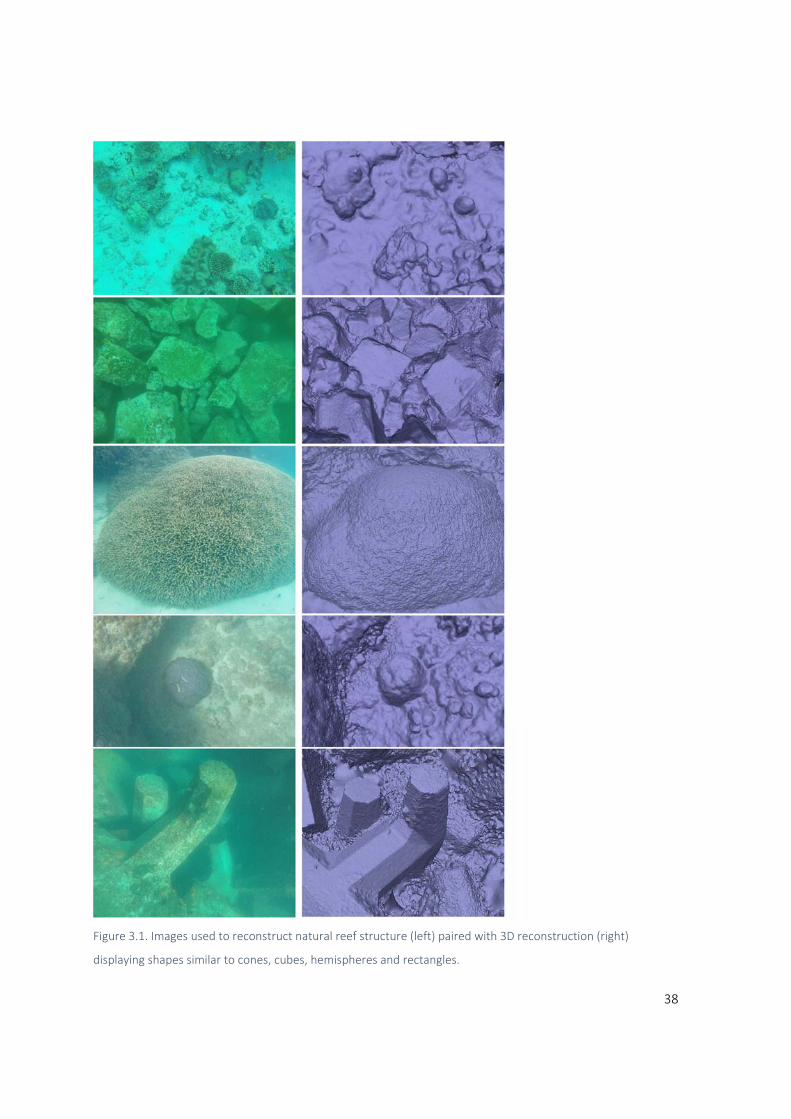
38  

 

Figure 3.1. Images used to reconstruct natural reef structure (left) paired with 3D reconstruction (right) 

displaying shapes similar to cones, cubes, hemispheres and rectangles. 

 

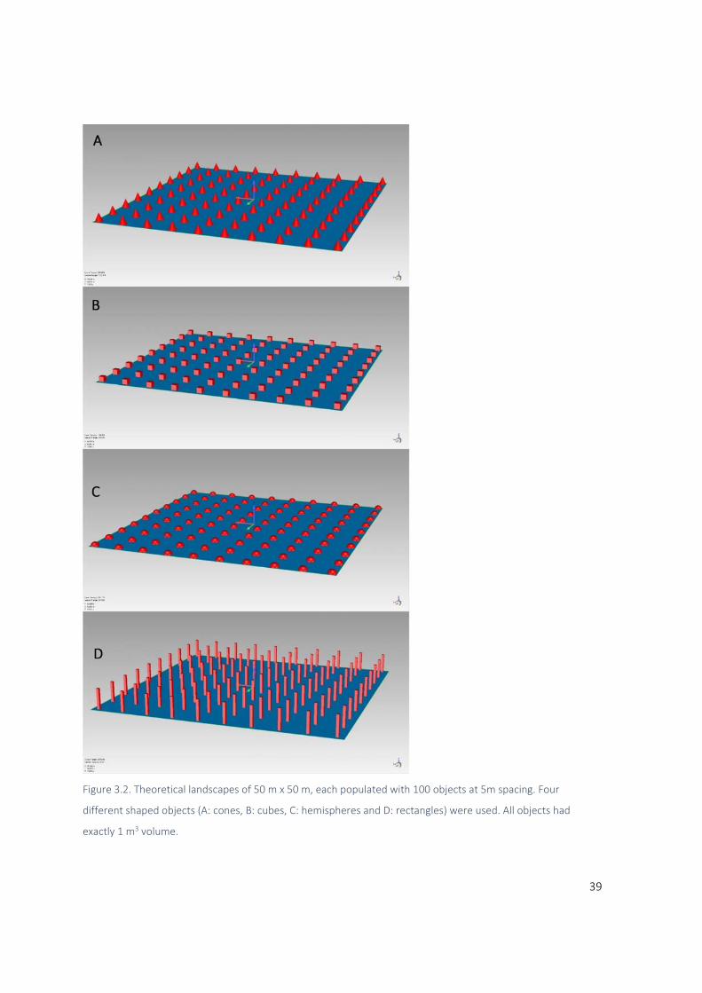
39  

 

Figure 3.2. Theoretical landscapes of 50 m x 50 m, each populated with 100 objects at 5m spacing. Four 

different shaped objects (A: cones, B: cubes, C: hemispheres and D: rectangles) were used. All objects had 

exactly 1 m3 volume.  

 

40  

3.2.1  Metric Validation 

There was generally good agreement between estimated and true values for all metrics Figure 3.3. 

rugosity xy and rugosity pobf were identical because all landscapes had zero landscape slope. Error 

rates (% difference from actual value) for calculated rugosity values were between 0.43% and 1.29% 

(Table 3.2). Averaged across all shapes, error rates for rugosity were +0.84%. Error rates for vertical 

relief were between 0% and 0.74%. Averaged across all shapes, error rates for vertical relief were ‐

0.23 %. Error rates for overhang were between 0% and 0.66%. Averaged across all shapes, error rates 

for overhang were +0.34%. Error rates for slope were 0% for all shapes. Despite these results being 

zero, it is important to include slope as a check because other variables depend on the orientation of 

the models. 

 

Figure 3.3. Measured levels of structural metrics (4 plots) from theoretical landscapes with different shaped 

objects (colours). Horizontal lines represent known levels of each metric for each landscape. 

 

 

41  

Table 3.2. Calculated structural metrics and known values for theoretical landscapes of different object shapes. 

 

 

Face angles were categorised into 10 degree bins from 0 (flat) to 90 (vertical). Non horizontal face 

angles for the landscape populated with cones was correctly apportioned to the 60‐70 degree 

category (true face angle of 66.16 degrees) (Figure 3.4). For landscapes populated with cubes non 

horizontal face angles were correctly apportioned to the 90‐100 degree category (90 degree vertical 

sides of cubes). For landscapes populated by hemispheres non horizontal face angles were distributed 

between 10 and 90 degrees reflecting the curved surface of a hemisphere. Non horizontal face angles 

in landscapes populated by rectangles were correctly apportioned to the 90‐100 degree category. 

Object Shape Known Calculated % error Known Calculated % error Known Calculated % error Known Calculated % error

Cone 1.1042 1.109 0.43 3.395 3.37 ‐0.74 0 0 0.00 0 0 0

Cube 1.16 1.168 0.69 2 2 0.00 0.1375 0.138 0.36 0 0 0

Hemisphere 1.0767 1.087 0.96 1.563 1.56 ‐0.19 0 0.001 na 0 0 0

Rectangle 1.32 1.337 1.29 8 8 0.00 0.2424 0.244 0.66 0 0 0

Rugosity Vertical relief Overhang Slope

 

42  

 

 

Figure 3.4. Polar plots visualizing the proportion of surface area in each surface angle category for each 

landscape. Surface area is binned in 10‐degree slope categories for A: cones, B: cubes, C: hemispheres, and D: 

rectangles.  

 

3.3   Deriving Feature Size 

While the above metrics are ecologically useful, this chapter aims to calculate the distribution of 

object sizes in a landscape. The following process was employed to separate objects in a landscape 

into size categories and calculate the amount of complexity contributed by each category.  

3.3.1  Resolution and Complexity 

As a complex surface is modelled at courser resolutions, features are smoothed over by links or pixels 

too large to resolve them. This decrease in resolution results in measured rugosity values decreasing 

to an asymptote near 1 (minimum possible rugosity) as resolution approaches quadrat size (Figure 

 

43  

3.5). Small objects are smoothed over first, then medium objects, then large objects are smoothed 

over. This allows rugosity to be measured with courser resolutions, calculating how much complexity 

is lost at each step. Then, by relating resolution to object sizes, the amount of complexity each object 

size contributed to the original rugosity can be calculated (Table 3.3). Note, this process does not 

distinguish between positive objects (e.g. a rock) vs. negative objects (e.g. a hole). It simply 

determines how much complexity is lost when these features are selectively excluded by resolutions 

too course to capture them. 

To describe the relationship between resolution and the size of objects lost, a sequential decimation 

process was conducted (see appendix “Complexity‐Metrics”). To capture the span of rugosity loss, 

resolutions were chosen between 0.04 m and 5.12 m. Resolutions were incremented in 1/3 log units 

such that when plotted on a logarithmic scale they were evenly distributed. The 4 theoretical 

landscapes were modelled at these resolutions to observe patterns in the loss of rugosity.  

 

44  

 Cone  Cube  Hemisphere  Rectangle 

0.04 m

 0.08 m

 0.16 m

 0.32 m

 0.64 m

 1.28 m

 2.56 m

 5.12 m

 

Figure 3.5. Visualization of complexity loss as objects are modelled at courser resolutions. Individual objects of 1 

m3 volume (in columns) from theoretical landscapes modeled at courser resolutions (in rows). Resolutions in 

metres are: 0.04, 0.08 , 0.16, 0.32, 0.64, 1.28, 2.56 and 5.12.  

 

45  

Table 3.3. Process for deriving object size. 1. Each landscape is modelled at courser resolutions and complexity is 

lost. 2. Complexity loss is standardized on a logistic curve, identifying the point of maximum complexity loss (Ȓ). 

3. Shapes in nature can be approximated by a range of geometric shapes. 4. Landscapes populated with 

geometric shapes (cones, cubes, hemispheres and rectangles) are modelled at courser resolution, identifying 

point of maximum complexity loss (Ȓ) for each. 5. This range of (Ȓ) values is used to derive an equation relating 

resolution to object size plus/minus the error introduced by different object shapes (Section 3.3 below). 

  Concept 

1  Measured complexity decreases as resolution gets courser 

 2  Resolution of maximum complexity loss (Ȓ) is 

found 

   3  Shapes in nature can be approximated by 

shapes with different surface area to volume ratios 

Photo:                         

3D model:                    

Shape:                          

4  Different shapes lose complexity at slightly different resolutions. This results in a range of Ȓ values for objects with the same volume but different shape 

 5  Different shapes are used to derive an equation 

relating resolution to object size (+/‐ 95% CI) Res. ∗ 3.410 7.37 1.49 Vol. 

 

46  

  With small increments of resolution change, objects do not disappear instantly, but are smoothed 

over gradually (Figure 3.6). Therefore, instead of calculating when an object is “gone”, it is more 

sensible to calculate at what resolution the object experiences maximum rugosity loss. 

 

Figure 3.6. Rugosity as a function of resolution for theoretical landscapes populated by different shapes. 1 m3 

landscapes shown here as example. For visualization cubes are shown modelled at the resolutions indicated on 

the x axis. 

 

Maximum rugosity loss was calculated by standardizing rugosity by initial (full resolution) rugosity at 

each landscape (as there are inherent differences in the overall max rugosity values for each 

landscape (Figure 3.6). A logistic curve was fitted to standardized data from each of the landscapes 

(cones, cubes, hemispheres and rectangles (Figure 3.7). The inflection point of each logistic curve was 

calculated and solved for x (resolution at maximum rugosity loss). This value is referred to as Ȓ and 

ranged from 0.38 m to 0.87 m resolution. Cubes consistently lost their rugosity at the finest 

resolutions while cones lost theirs at the coarsest resolutions. 

 

47  

 

Figure 3.7. Rugosity (standardized as proportion full rugosity) as a function of resolution. Data fit with logistic 

curve (coloured lines) modelling rugosity loss for each object shape. The point of maximum rugosity loss (Ȓ) is 

indicated by vertical dashed line. 

 

The range of Ȓ values was used as a proxy for the inherent variability of shapes in natural 

environments. To achieve this, Ȓ values were divided by the cube root of the object’s volume (its 1D 

size) giving the ratio of resolution to object size at the point of maximum rugosity loss. The mean and 

variance of the resulting Ȓ/1D value was calculated among object shapes (Table 3.4). The resulting 

mean Ȓ/1D (+/‐ 95% confidence interval from variance among object shapes) is the resolution at 

maximum rugosity loss for any feature in the range of cubes, cones, hemispheres and rectangles. It is 

known that objects of different shapes have different length to volume ratios. Therefore, the 95% 

confidence intervals are expected to be wide. This intentionally reflects the variability of objects that 

will be mapped in the future. 95% confidence intervals will inform the spacing of object size categories 

in the final analysis. 

 

48  

Table 3.4. Variance of Ȓ/1D values among object shapes (cones, cubes, hemispheres and rectangles). Ȓ/1D is 

calculated by dividing the resolution at maximum rugosity loss by the cube root of the object volume (i.e. the 

object’s 1D size). 

  

 

The coefficient of variation of Ȓ/1D among object shapes was CV = 0.325. The 95% confidence interval 

was 0.212. Overall Ȓ/1D +/‐ 95% confidence interval was Ȓ/1D = 0.664 +/‐ 0.212 (from this point 

forward, the 95% CI will be replaced by these derived numbers). This means that the average shape 

will experience its maximum loss in rugosity at a resolution that is 0.664 of its generalised 1D size.  

This relationship is generalized to objects with height to base ratios and surface area to volume ratios 

in the range of the cones, cubes, hemispheres and rectangles used to derive this equation.  

3.3.2  From Complexity loss to Object Size 

To approximate the size of objects in a landscape using their 1D size, we must explore the relationship 

between the 1D size (resolution) and the 3D size (volume) of objects. In general, the way volume is 

calculated is by cubing an object’s length and multiplying by a constant specific to the object’s shape. 

This allows us to know an objects 3D size (volume) by knowing its 1D size (length). For example, the 

constant relating a cube’s length to its volume is 1, so the volume of a cube with edge length E is 

simply Vol = 1 * E3. The constant relating a sphere’s length (radius) to its volume is 4/3π or about 4.19, 

so the volume of a sphere is Vol = 4.19 * r3. This principle is true of all 3D objects, but the constant is 

different for different shapes and of course the edge distances may vary (e.g. rectangles). 

The objective in this step is to derive a general equation which allows us to use the resolution (1D size) 

at which mapped features disappear to infer the approximate volume (3D size) of those features. This 

can be expressed as Equation 1. 

Equation 1. Generalized formula relating resolution to volume for any shape. 

Resolution ∗ Constant Volume        (Equation 1) 

Shape Ȓ/1D

1 m3 Cone 0.87

1 m3 Cube 0.38

1 m3 Hemisphere 0.80

1 m3 Rectangle 0.63

Variance (CV) 0.325

Mean Ȓ/1D  0.664

Mean 95% CI 0.212

 

49  

 

The objective is not to precisely calculate the volume of all features, but to group features into broad 

size bins of ecological importance (i.e. distinguishing between coral fingers and boulders and drop‐

offs). Importantly, the variance among these shapes is also carried through the calculations and 

included in the final equation. 

Once resolutions are related to rugosity loss for the four shapes with 95% CI, it is possible to calculate 

a generalized constant C that relates resolution to the volume of unknown objects (in the range of 

those used above). This is done using Equation 2. Ȓ/1D and Vol are known, allowing C to be solved for. 

The 95% confidence intervals are carried through to C by calculating C at the upper and lower bounds 

of Ȓ/1D. This results in a constant “C +/‐ 95%” that relates the length of shapes (in the range of those 

used here) to a measure of their generalised volume. 

Equation 2. Solving for the constant C relating 1D size to 3D size of objects. Ȓ /1D is the point of maximum 

complexity loss divided by the 1D size of objects. Vol is the known volume of objects (1 m3). 

Ȓ/1D Vol      (Equation 2) 

0.664 / 0.212 1 

C 3.410 7.37/ 1.49  

 

Using the established constant C, I was a then able to convert resolution to feature size using Equation 

3. Volume can be approximated by cubing any resolution, and multiplying by 3.41 (+/‐), assuming 

objects are (on average) in the range of cones, cubes, hemispheres or tall rectangles. 

Equation 3. Relating resolution to volume with asymmetrical 95% confidence interval. 

Res. ∗ C Vol.      (Equation 3) 

   Res. ∗ 3.410 7.37 1.49 Vol. 

 

3.3.3  Object size validation  

Using Equation 3, the original 4 landscapes were analysed for object size distribution. Resolution bins 

were: 0.03 ‐ 0.08, 0.08 ‐ 0.16, 0.16 ‐ 0.32, 0.32 ‐ 0.64, 0.64 ‐ 1.3, 1.3 ‐ 2.6, 2.6 ‐ 5.2 and 10 – 13 metres. 

 

50  

Object size analysis was sensitive to object shape, resulting in a spread of peaks for rugosity 

contributed by different shaped objects (coloured lines in Figure 3.8). When comparing the known 

peaks to the mean (and 95% CI) object size estimated the process above from the volume of cubes 

was consistently underestimated while the volume of hemispheres was consistently overestimated. 

When data for all objects were combined, a peak at 1 m3 was evident (black line in Figure 3.8) which is 

very close to the estimated object size value. 95% confidence intervals were calculated using the 

confidence around C (plotted in grey). 

 

Figure 3.8. Rugosity contributed by 1 m3 objects. Object size analysis of the 4 theoretical landscapes (red = 

cones, green = cubes, turquoise = hemispheres, purple = rectangles). Each is modelled by loess moving average 

lines to aid visualization. Black curve models average of all landscapes. Grey curves model 95% CI’s. Dashed 

vertical lines indicate object size with 95% CI’s. 

 

To further test object size analysis, two new landscapes of 8 m3 objects and 0.125 m3 objects were 

created for each shape, resulting in a total of 12 landscapes. Each new landscape shared the same 

 

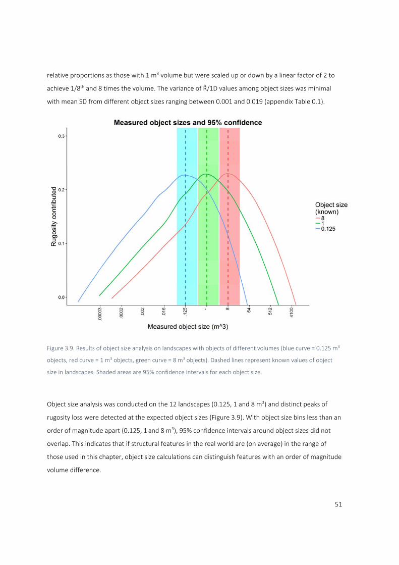
51  

relative proportions as those with 1 m3 volume but were scaled up or down by a linear factor of 2 to 

achieve 1/8th and 8 times the volume. The variance of Ȓ/1D values among object sizes was minimal 

with mean SD from different object sizes ranging between 0.001 and 0.019 (appendix Table 0.1).  

 

Figure 3.9. Results of object size analysis on landscapes with objects of different volumes (blue curve = 0.125 m3 

objects, red curve = 1 m3 objects, green curve = 8 m3 objects). Dashed lines represent known values of object 

size in landscapes. Shaded areas are 95% confidence intervals for each object size. 

 

Object size analysis was conducted on the 12 landscapes (0.125, 1 and 8 m3) and distinct peaks of 

rugosity loss were detected at the expected object sizes (Figure 3.9). With object size bins less than an 

order of magnitude apart (0.125, 1 and 8 m3), 95% confidence intervals around object sizes did not 

overlap. This indicates that if structural features in the real world are (on average) in the range of 

those used in this chapter, object size calculations can distinguish features with an order of magnitude 

volume difference.  

 

52  

3.4  Discussion 

This chapter presents methodology for the systematic derivation of standard as well as novel metrics 

to assess the structural complexity represented within 3D models of landscapes. The metrics derived 

are available via a software package and the analyses presented here suggest this package accurately 

calculates surface rugosity, vertical relief, vertical surface, slope and the distribution of face angles in 

3D models. Importantly, the approach presented here allows the direct assessment of complexity 

contributed by different object sizes in 3D models, marking a new step in the progression of structural 

analysis for ecology.  

Despite being conducted on theoretical landscapes, there were several sources of error present in 

these analyses. Rugosity was likely overestimated because of dropped triangles around the edges of 

virtual quadrats. At least 75% of every triangle had to fall within a virtual quadrat to be calculated as 

part of the rugosity. This likely resulted in minor edge effects, reducing the calculated rugosity values 

and contributing to the roughly 1% under‐estimation of rugosity as compared to known values. There 

was an artefact of the resolution‐reduction process whereby the right angles on the cubes and 

rectangles interacted with the grid of large triangles, introducing some variability in the way squares 

and rectangles lost their complexity. This is not likely to apply to natural landscapes as regularly 

spaced objects with right angles are rare. Vertical faces were well captured by the 90‐100 degree face 

angle bin however this resulted in vertical areas being calculated as “overhang”. This will not be an 

issue in natural environments as perfectly vertical flat surfaces are exceedingly rare. 

This object size analysis in this chapter is not intended for precise calculations of the volume of objects 

with unknown shape. That would be impossible. It is, however, valid to use the derived equation to 

approximate the size of objects, grouping them in broad categories of volume. The shapes used in this 

chapter represent a wide range of surface area to volume ratios. This range is intentionally wide and 

informed the confidence intervals around object size categories. The 95% confidence intervals 

calculated based on the cones, cubes, hemispheres and tall rectangles used in this study indicate that 

object size bins should be at least 8‐fold apart (i.e. 1 m3, 8 m3, 64 m3) in order to be uniquely 

characterised. In other words, this equation would distinguish a car from a washing machine or an 

apple from a soccer ball. Dividing objects into 8‐fold or even 10‐fold volume bins across multiple 

orders of magnitude still marks a significant advance in the ecological questions that can be asked 

with structural complexity data.  

 

53  

The range of feature sizes that can be calculated in a landscape will always be limited by the 

quadrat/transect size on the upper bound, and by resolution on the lower bound. The extent and 

resolution of 2.5D and 3D data from natural landscapes is already enough to calculate ecologically 

important ranges of complexity at different scales (Friedman et al. 2012; Figueira et al. 2015; 

Ierodiaconou et al. 2018). With ever increasing spatial data acquisition and computational power the 

utility of digital measures of cross‐scale structure in ecology is likely to expand. While the fractal 

dimension is a useful framework for generalising cross‐scale trends in structures(Frost et al. 2005), it 

does not present data that are easily interpreted by managers of engineers likely to be designing 

habitats. In fact, in some cases, expressing structurally explicit measurement as fractal dimensions can 

actually obscure the ecological utility of hard‐earned measurements (Nash et al. 2013; Young et al. 

2017). The methods in this chapter for calculating object sizes outline an alternative and structurally 

explicit avenue from fractal dimension. 

The Textural Discontinuity Hypothesis (Holling 1992), postulates that refugia are discontinuously 

distributed across scales in natural landscapes and that this drives observed “clumpyness” in animal 

body sizes. Empirical data to test this hypothesis have been difficult to acquire at high resolution and 

across multiple spatial scales. This has been exceptionally acute at marine environments where 

measurement is inherently difficult. The methods presented in this chapter should provide data on 

the (dis)continuity of structure across multiple orders of magnitude and at resolutions relevant to fish 

assemblages.  

This approach provides structurally explicit metrics of complexity, increasing the utility of structural 

analysis for habitat creation (Loke et al. 2015). Moving beyond summary metrics like rugosity and 

fractal dimension to more structurally and spatially explicit metrics like object size enables these 

analyses to be directly implemented in eco‐engineering and artificial reef design. In the following 

chapters of this thesis the methods from this chapter will be used to analyse a range of marine reef 

habitats for metrics of structural complexity. The resulting structural analysis will be used to address 

questions of fish habitat use, informing ecological theory and habitat design. 

3.4.1  Conclusion 

The methods and formulae for analysis of 3D data outlined in this chapter provide a standardized 

approach to calculating a suite of commonly used and ecologically important metrics of habitat 

structural complexity. The approach is shown to be sufficiently accurate in all metrics. Additionally, an 

 

54  

entirely new metric of habitat structural complexity is calculated, potentially allowing marine mapping 

to directly inform eco‐engineering practices and ecological theory. 

 

55  

Chapter 4: Exploring structural niche space in benthic habitats using 

3D modelling 

 

Summary: 

1. The physical shape or structure of a habitat is a key driver of species’ distributions and central 

to ecological niche differentiation. Ecological niche theory would imply that a contributing 

factor to the striking richness and abundance of coral reefs is the abundance of small physical 

niches in these environments. 

2. Here I employ the suite of metrics described in Chapter 3 to test hypotheses about the 

structure of four related, but distinct habitat types: rocky reef, coral reef slopes, coral reef 

patches, and anthropogenic breakwaters. 

3. Face angle distribution was variable on rocky reefs, but relatively consistent at breakwalls and 

consistently steeper at coral slopes and coral patches. Breakwall habitat contains significantly 

more features in the 1.7 m3 (roughly refrigerator size) range while coral habitats have high 

density of small features. 

4.  Structural analysis confirms the extreme levels of complexity contributed by small objects at 

coral reefs. 

4.1   Introduction 

The structural complexity of habitats is an important driver of species distribution (MacArthur and 

MacArthur 1961; Graham and Nash 2013). Developing a mechanistic understanding of this 

relationship is important, especially in the context of unprecedented changes to habitat structural 

complexity in the Anthropocene (Wernberg et al. 2012). Climate change and coral mortality 

associated with bleaching (Hughes et al. 2017), along with shoreline armouring (Mayer‐Pinto et al. 

2017) are expected to change the structural complexity of marine habitats by removing high‐

complexity coral habitats and mangroves and increasing vertical structures. Limitations around the 

measurement of habitat structure have led to summary metrics being commonplace in ecology 

(Kovalenko et al. 2012). These metrics generally assume complexity to be linear across scales (e.g. 

fractal dimension) or homogenous in object sizes (e.g. surface rugosity) (see chapter 1 of this thesis). 

In many circumstances, these summary metrics are appropriate to the question at hand. Developing a 

 

56  

mechanistic understanding of the relationship between habitat structural complexity and ecological 

responses, however, is increasingly important for many applications from modelling the impacts of 

climate change to informing eco‐engineering and artificial reef construction. To inform these pursuits, 

detailed capture and analysis of structure is critical. 

One framework for conceptualizing the importance of detailed metrics of structure is the textural 

discontinuity hypothesis (TDH) (Holling 1992). The TDH is based on 2 premises: (1) animal body sizes 

are driven by the size of physical refugia in a landscape; and (2) the distribution of refuge size in 

landscapes is uneven or discontinuous. Holling paired these two ideas to explain the observed 

“clumpyness” of animal body size distributions in nature. There is strong evidence in marine 

environments for the first part of the TDH, linking body size to refuge size. Complexity at the scale of 

coral colonies is linked to the abundance of small to medium sized fishes (Rogers et al. 2014), and loss 

of fine habitat structure from coral has been shown to result in fewer small fishes locally (Wilson et al. 

2010). The second premise about discontinuity is fairly intuitive when one compares a rocky reef with 

relatively smooth surfaces and steep drop‐offs to a coral reef with its enormous number of small 

refugia as well as drop‐offs. But surprisingly, evidence for this second part of the TDH is relatively 

scarce. This is likely in part due to the fact that collecting those data at relevant scales is difficult, 

especially under water. This difficulty is compounded by a lack of suitable metrics to express such 

discontinuity even when it is measured (Loke et al. 2015). 

The most commonly used metric of structural complexity in marine ecology is linear rugosity (Risk 

1972; Kovalenko et al. 2012). Rugosity, being a ratio of fitted to linear distance, contains no 

information about object sizes. The fractal dimension (Mandelbrot 1982) is another metric of 

complexity which moves in the direction of quantifying object sizes in a landscape. Fractal dimension 

is based on the idea that the perceived length of a complex line depends on the size of the ruler used 

to measure it. The larger the ruler, the more small complexity will be ignored. In ecology the slope of 

this “ruler‐to‐distance” relationship is used as a measure of complexity at different scales or 

resolutions. Nash et al. (2013) quantified complexity on a reef at 3 scales, yielding 2 fractal dimension 

values (small to medium and medium to large), and found that small bodied fishes were linked to 

smaller reef features. More recently, technological advances such as computer vision and 

photogrammetry have enabled metrics of structure to be efficiently calculated at multiple scales 

(Friedman et al. 2012; Ferrari et al. 2016b) . Multi‐scale rugosity has been linked to coral recovery 

 

57  

(Ferrari et al. 2016a) and fish abundance (Roberts and Ormond 1987), suggesting that these metrics 

are ecologically important. 

Different phenomena drive the habitat structural complexity of different ecosystems. Coral reefs are a 

biogenic habitat typically considered highly structurally complex (Luckhurst and Luckhurst 1978; 

Knudby and LeDrew 2007). At rocky reefs, in contrast, the habitat structural complexity is primarily 

driven by a‐biotic rock substrate. Like coral reefs, rocky reefs often support rich and abundant benthic 

assemblages that influence the structure of the local fish assemblages (Trebilco et al. 2015). 

Breakwalls are comparable to rocky reefs and coral reefs in that they provide habitat to rich and 

abundant fish assemblages (Chapter 2 of this thesis). However, because they are engineered 

structures, they provide a habitat structurally distinct from natural reef (Firth et al. 2014). Another 

result of the anthropogenic nature of breakwalls is their homogeneity across the whole structure 

(author’s personal observation). 

Numerous studies have claimed that landscapes in nature are fractal, meaning that their complexity 

remains constant as spatial extent and resolution scale together (Sugihara and May 1990). However, 

Halley et al. (2004) questioned the existence of such a relationship, pointing out that many landscapes 

do not conform to it. But perhaps more importantly, the TDH implies that it is specifically the 

departures from a linear relationship between scale and complexity (the discontinuities) that are 

important ecologically. While natural reefs may or may not be truly fractal, there is no reason to 

presume that anthropogenic structures would conform to this phenomenon of scale invariant 

complexity. In fact, breakwalls are usually built of cast concrete hanbars or tetrapods (Gürer et al. 

2005) and concrete blocks. These distinct structures provide an interesting extreme case for object 

size distributions in a landscape. 

Niche differentiation theory provides a different perspective on habitat use from the TDH. Niche 

differentiation tells us that a high density of physical niches facilitates increased abundance and 

diversity of animals. These patterns have been observed on coral reefs (Sale 1977; Luckhurst and 

Luckhurst 1978). The TDH predicts that animals respond to complexity at scales relevant to their body 

size and that the distribution of object or refuge sizes is important. There is some evidence for this 

discontinuity existing in marine environments such as coral reefs (Knudby and LeDrew 2007). Taken 

together, these two theories could provide a more complete picture of how habitats drive species 

distributions. But evidence of, and indeed metrics to describe the object size makeup of different 

habitat types is lacking. Quantifying the characteristics of different reef habitat types, including object 

 

58  

sizes or textural (dis)continuity is fundamental to understanding the relationship between habitats 

and ecology. Information on object size distributions spanning meaningful ranges of resolution and 

spatial extent would contribute to several broad ecological goals. These data could underpin tests of 

ecological theory such as the TDH. Structural data could also be incorporated into predictive models 

of ecological responses to climate change, especially at coral reef environments. And finally, the 

explicit measurement of object size distributions and 3D capture of structure moves ecology closer to 

engineerable measures of habitat structural complexity for application in eco‐engineering.  

In this chapter I extract the structure metrics detailed in chapter 3 of this thesis from four real‐world 

habitats (coral slopes, coral patches, rocky reefs and breakwalls) to achieve the following aims: 

A. Examine reef types for differences in structural character. 

B. Examine reefs for cross scale discontinuity (differences in object size distributions). 

C. Explore theories of biodiversity in the context of detailed structural complexity. 

Specifically, I hypothesize the following differences among reef types will be evident: 

1. Reef types will be differentiated by their levels of structural complexity with coral habitats 

being similar to each other and distinct from rocky reef and breakwall habitats, which will be 

distinct from each other. 

2. Anthropogenic breakwall habitat will be less structurally variable than the other habitat types. 

3. Distributions of object sizes will differ among habitat types with coral transects having more 

small objects. 

4.2   Methods 

79 transects from 4 habitat types were mapped and analysed for metrics of habitat structure. Habitat 

types were breakwall (BW, n = 12), coral patches (CP, n = 18), coral slopes (CS, n = 15) and rocky reefs 

(RR, n = 34) (Figure 4.1). Breakwall and rocky reef transects were from Botany Bay and Port Kembla, 

each of which had 6 BW transects and 17 RR control transects (these are the same transects 

described in Chapter 2 of this thesis). Coral transects were imaged at One Tree Island and Heron 

Island on the Southern Great Barrier Reef. CP transects were inside reef lagoons and ran along the 

side of a coral bommie between 1 and 5 m depth. CS transects were areas of reef outside the reef 

crest, taken along an isobath at between 3 and 12 m depth and with a slope range of 15 – 60 degrees.  

All transects were 25 x 10 m. 

 

59  

 

Figure 4.1. Typical sections of each habitat type. Breakwall (A), coral patch (B), coral slope (C), and rocky reef (D). 

Images taken from 3D reconstructions. 

 

4.2.1  Mapping 

Mapping and 3D mesh reconstruction were conducted as described in Figueira et al (2015). This 

method involved systematically capturing several thousand still images of each transect and 

reconstructing the shape of the substrate using photogrammetry. The method is precise to 3 cm and 

generates digital reconstructions of habitats. In addition to being an extremely high‐resolution 3D 

capture method, this approach yields full 3D models which include overhanging surfaces (i.e. not 2.5D 

raster data). Each digitally captured transect was scaled using a minimum of 2 scale features and 

 

60  

oriented to real‐world up. Areas of obviously bad mesh and any visually apparent edge effects were 

removed and holes of <2m diameter filled using the fill with flat surfaces tool in CAD software 

Geomagic Studio. Models were standardized to approximately 8,000 triangles per m2 yielding triangle 

size of approximately 3cm edge length and roughly 2 million triangles in a model of a 25 m x 10 m 

transect. 

4.2.2   Data extraction 

Reefs transects were analysed with the “complexitymetrics” software described in chapter 3. This 

resulted in 4 univariate metrics of structure (surface rugosity, vertical relief, percent overhang and 

slope) as well as 2 distribution metrics (face angle distribution and object size distribution). For each 

transect, the proportion of surface area in each face angle bin was calculated, creating a distribution 

of face angles. A process of controlled sequential decimation (resolution reduction) was conducted to 

calculate the amount of surface rugosity contributed by each object size bin, creating a distribution of 

object sizes. Resolutions were chosen on a log (2) scale between maximum resolution and the largest 

triangles that would fit on transects. This resulted in the original landscapes being modelled with 0.05, 

0.1, 0.2, 0.4, 0.8, 1.6, 3.2, 6.4 and 12.8 million triangles. By accounting for the unknown shape of real‐

world objects and testing which object sizes are lost at these resolutions a formula was derived linking 

resolutions to object sizes (see Chapter 3). The resulting 9 object size categories were centred on the 

following volumes: 0.0004, 0.003, 0.02, 0.2, 1.7, 14, 110, 890 and 7200 (m3). Object size data were 

displayed in two ways. First the surface rugosity contributed by each object size to the total surface 

rugosity was plotted. Then standardised object size distribution curves were created by dividing the 

object size contributions for each transect by the initial surface rugosity of that transect. This latter 

approach allows comparison of the relative frequency of object sizes amongst transects, decoupled 

from the absolute magnitude of surface rugosity, which does vary amongst transects. The result was 6 

metrics of habitat structure (surface rugosity, vertical relief, percent overhang, slope, face angle 

distribution, and object size distribution). 

4.2.3   Statistical analysis 

Statistical analysis was conducted with the software package R v3.4.0 (Team 2013). To investigate 

differences among the six complexity metrics (surface rugosity, vertical relief, overhang, slope, surface 

steepness and object size) among the four habitat types (BW, CS, CP and RR) Analyses of Variance 

(ANOVA) in package stats (Team 2013) was used. A separate ANOVA was run for each of the six 

complexity metrics, with habitat type as the sole explanatory variable and transects as replicates. 

 

61  

Assumptions of normality and heteroscedasticity were tested using Shapiro‐Wilk test (Royston 1982) 

and Levene’s test respectively. Where data did not meet the assumption of homoscedasticity, non‐

parametric ANOVAs were conducted using Kruskal‐Wallis tests and Dunn’s post hoc tests with 

Bonferroni corrections for multiple comparisons. This test compared median values, rather than mean 

values as in standard parametric ANOVAs. Tukey HSD post‐hoc tests were used with p‐values adjusted 

for multiple comparisons. 

Individual metrics were visually displayed with boxplots. Additionally, transects were plotted in 

multivariate space with Principal Component Analysis (PCA) using all 6 structure metrics. PCA allows 

the vectors of each structure metric to be displayed, illustrating the differences in metric composition 

of each transect and among habitat types. Multivariate compositions of each transect were compared 

among habitat types by permutational multivariate ANOVA using the ‘Adonis’ function in the package 

vegan 2.4‐5 (Dixon 2003) with Bonferroni adjusted p values for multiple comparisons. 

To test hypotheses about variability of structure metrics at different habitat types, dispersion of 

transects multivariate position was calculated using the ‘betadisper’ function in the r package vegan. 

This function implements Marti Anderson’s PERMDISP2 function (Anderson 2004) to calculate 

multivariate dispersion. Dispersion data were compared among habitat types using ANOVA. 

Data on surface angle distribution and object size distribution were represented by distribution curves 

as well as non‐metric multi‐dimensional scaling (nMDS) plots. nMDS is similar to PCA in that it 

positions transects in multi‐dimensional space, visualising their differences. nMDS was chosen for 

surface angle and object size distributions because of the prevalence of zeros in these datasets. To 

test hypotheses about relative proportions of object sizes in transects, object size distributions were 

calculated at each transect and the skewness of these distributions was calculated using the R 

package moments v.14 (Komsta and Novomestky 2015). This routine evaluates the central tendency 

of a distribution (e.g. object sizes) and expresses it as more or less skewed towards large objects. This 

test was performed to establish the relative amount of large, medium or small objects (in the case of 

object sizes) and the relative amount of “upward”, “vertical” or “downward” facing surfaces (in the 

case of surface angles). ANOVA was then used to compare the skewness of distributions among reef 

types, with assumptions of normality and homoscedasticity tested as above. 

 

62  

4.3   Results 

79 transects between 164 m2 and 544 m2 planar area were captured at native resolutions between 

8,000 and 40,000 triangles per m2. These were standardized to roughly 8,000 triangles per m2 and 

analysed for 6 metrics. Object size analysis returned results for objects between 0.0004 m3 and 7200 

m3 for all habitat types. At 23 of the 79 transects the largest object size was not calculated due to the 

overall transect size being too small to accommodate this coarse resolution.  

Examples of 3D captured reef habitats are available for viewing on Sketchfab.com at the following 

links: 

Breakwall: https://sketchfab.com/models/00f90332ba9f4a8db61a61b60ef7b0bf 

Coral Slope: https://sketchfab.com/models/9cb8643835d74a32b1de7096cbb423b7 

Coral Patch: https://sketchfab.com/models/98fe62762eef4b449e0c98b6e1227949 

Rocky Reef: https://sketchfab.com/models/0f647c2dbe584f57a8cec351103be569 

4.3.1   Structure metrics 

Values for overhang, face angle skewness and object size skewness were normally distributed. Values 

for slopes, vertical relief and face angle skewnesses were not normally distributed, as indicated by 

significant Shapiro‐Wilk normality tests. These data were not transformed as ANOVA is robust to non‐

normality when sample sizes are large, as is the case here (Underwood 1997). Values for overhang, 

face angle skewnesses and object size skewnesses were heteroscedastic as indicated by significant 

Levene’s tests. Non‐parametric ANOVAs were used in these instances. 

ANOVA results for differences among habitat types were significant for all 6 metrics (Table 4.1 and 

 

Table 4.2). Pair‐wise tests of surface rugosity indicated three groups with BW habitat significantly 

more rugose than CP and CS, which were significantly more rugose than RR (Table 4.3 for summary 

and Appendix 4.1 and Appendix 4.2 for full results). Pair‐wise tests on vertical relief indicated two 

groups with BW habitat having significantly more vertical relief than CP, CS and RR Pair‐wise tests of 

overhang indicated that BW had significantly more overhang than RR and CP but was not significantly 

different from CS. CS and CP were similar, and RR had significantly less overhang than BW or CS. Pair‐

 

63  

wise tests on slope indicated two groups with BW significantly more sloped than CP, CS and RR. 

Correlation of metrics ranged from <0.1 to 0.92 R2 (Appendix 4.3). 

Table 4.1. Differences in 3 structure metrics (surface rugosity, vertical relief and slope) among habitat types as 

tested by ANOVA. 

Metric  Factor  Df  SS  MS  F  p 

Surface Rugosity  habtype  3  4.66  1.55  26.1  << 0.01 

  Resid  72  4.28 0.06

Vertical relief  habtype  3  135.6 45.19 24.0 << 0.01

  Resid  72  135.5  1.88 

Slope  habtype  3  1733  577.5  13.2  << 0.01 

   Resid  72  3163  43.9       

 

 

Table 4.2. Differences in 3 heteroscedastic structure metrics (overhang, face angle distribution and object size 

distribution) among habitat types as tested by Non‐parametric ANOVA. 

Metric  Factor  Df  chi‐squared  p 

Overhang  habtype  3  30.44  << 0.01 

Face Angle Dist.  habtype  3  38.8  << 0.01 

Object Size Dist.  habtype  3  43.12  << 0.01 

 

 

64  

 

Figure 4.2. Boxplots of structure metrics for 4 habitat types (red = breakwall, blue = coral patch, green = coral 

slope, purple = rocky reef). Boxplots show median, first and third quartiles (box) range of data (points) and data 

within 1.5 inter quartile range of median (whiskers). Structure metrics are, A: surface rugosity, B: vertical relief, 

C: overhang and D: slope. Each point = 1 transect. Grey letters indicate significantly different (p<0.05) groups 

based on post‐hoc tests. Plot A: BW > CS and CP > RR, Plot B: BW > CP, CS and RR, Plot C: BW > CP and RR, RR < 

CS and BW. Plot D: BW > CS, CP and RR. 

 

 

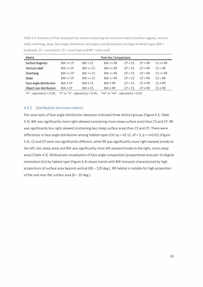
65  

Table 4.3. Summary of Pair‐wise post‐hoc results comparing size structure metrics (surface rugosity, vertical 

relief, overhang, slope, face angle distribution and object size distribution) amongst 4 habitat types (BW = 

breakwall, CP = coral patch, CS = coral slope and RR = rocky reef).  

Metric  Post‐Hoc Comparisons

Surface Rugosity  BW >> CP  BW > CS  BW >> RR  CP = CS  CP > RR  CS >> RR 

Vertical relief  BW >> CP  BW >> CS  BW >> RR  CP = CS  CP = RR  CS = RR 

Overhang  BW >> CP  BW >> CS  BW >> RR  CP = CS  CP > RR  CS >> RR 

Slope  BW >> CP  BW >> CS  BW >> RR  CP = CS  CP = RR  CS = RR 

Face angle distribution  BW ≠ CP  BW ≠ CS  BW ≠ RR  CP = CS  CP ≠ RR  CS ≠ RR 

Object size distribution  BW ≠ CP  BW ≠ CS  BW ≠ RR  CP = CS  CP ≠ RR  CS ≠ RR 

"=" : adjusted p > 0.05,    ">" or "<" : adjusted p < 0.05,    ">>" or "<<" : adjusted p < 0.01 

 

4.3.2  Distribution structure metrics 

Pair‐wise tests of face angle distribution skewness indicated three distinct groups (Figure 4.3, Table 

4.3). BW was significantly more right‐skewed (containing more steep surface area) than CS and CP. RR 

was significantly less right‐skewed (containing less steep surface area) than CS and CP. There were 

differences in face angle distribution among habitat types (Chi sq = 43.12, df = 3, p = <<0.01) (Figure 

4.3). CS and CP were not significantly different, while RR was significantly more right skewed (mode to 

the left; less steep area) and BW was significantly more left skewed (mode to the right; more steep 

area) (Table 4.3). Multivariate visualization of face angle composition (proportional area per 10 degree 

orientation bin) by habitat type (Figure 4.4) shows trends with BW transects characterized by high 

proportions of surface area beyond vertical (90 – 120 deg.). RR habitat is notable for high proportion 

of flat and near‐flat surface area (0 – 10 deg.).  

 

 

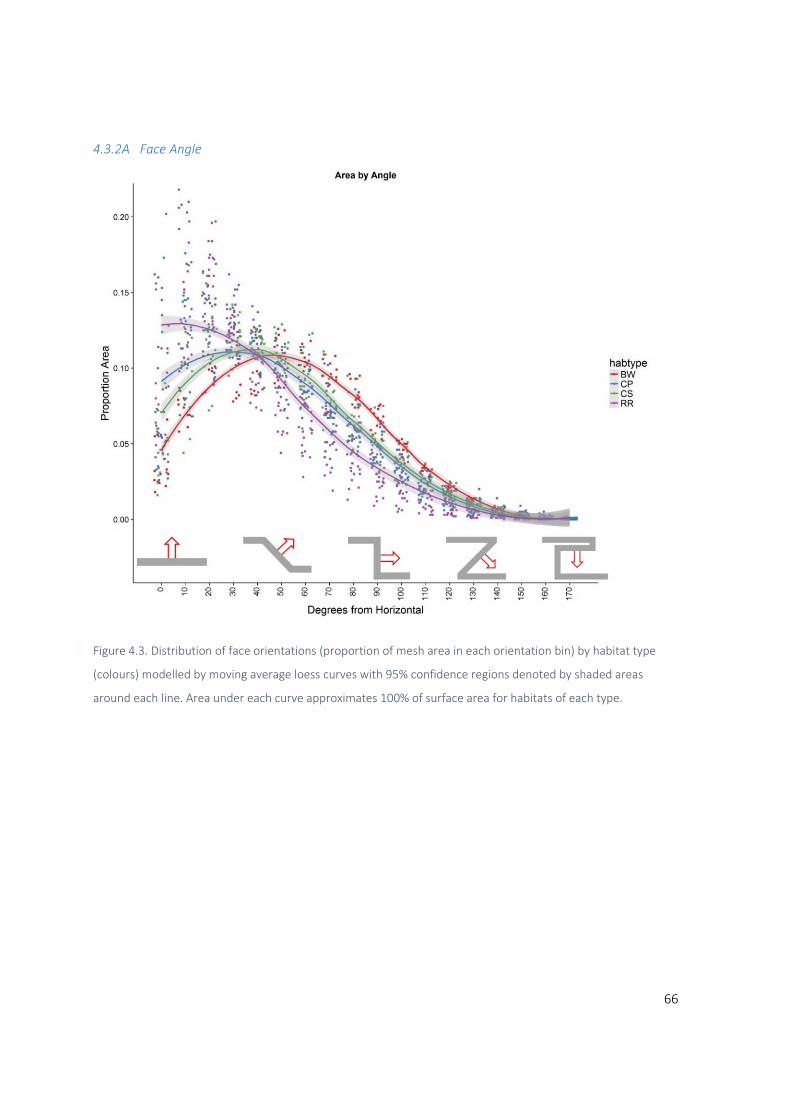
66  

4.3.2A  Face Angle 

 

Figure 4.3. Distribution of face orientations (proportion of mesh area in each orientation bin) by habitat type 

(colours) modelled by moving average loess curves with 95% confidence regions denoted by shaded areas 

around each line. Area under each curve approximates 100% of surface area for habitats of each type. 

 

 

67  

 

Figure 4.4. Multivariate visualization of differences among the composition of face angles at different habitat 

types (colours). Grey annotations indicate the loadings of each face angle bin such that transects closer to a grey 

number have relatively more of that face angle. 

 

4.3.2B  Object Size 

Tests on skewness of object size distributions were conducted on the non‐standardized distribution 

data. While standardizing distributions across habitat types is important to visualize differences 

among habitats, it does not change the shape (specifically mode or skewness) of distribution curves 

(Figure 4.5, Figure 4.6). There were significant differences in object size composition among habitat 

types (F = 4.53, df = 3, p = <0.001). Pair‐wise tests of object size distribution indicated two distinct 

groups. CS and CP were similar to each other (H= ‐1.61, df= 1, p = 0.321) and both were significantly 

more right‐skewed (i.e. modes to the left; containing more small objects) than RR and BW which were 

similar to each other (H= ‐2.20, df= 1, p = 0.084) (Figure 4.7).  

 

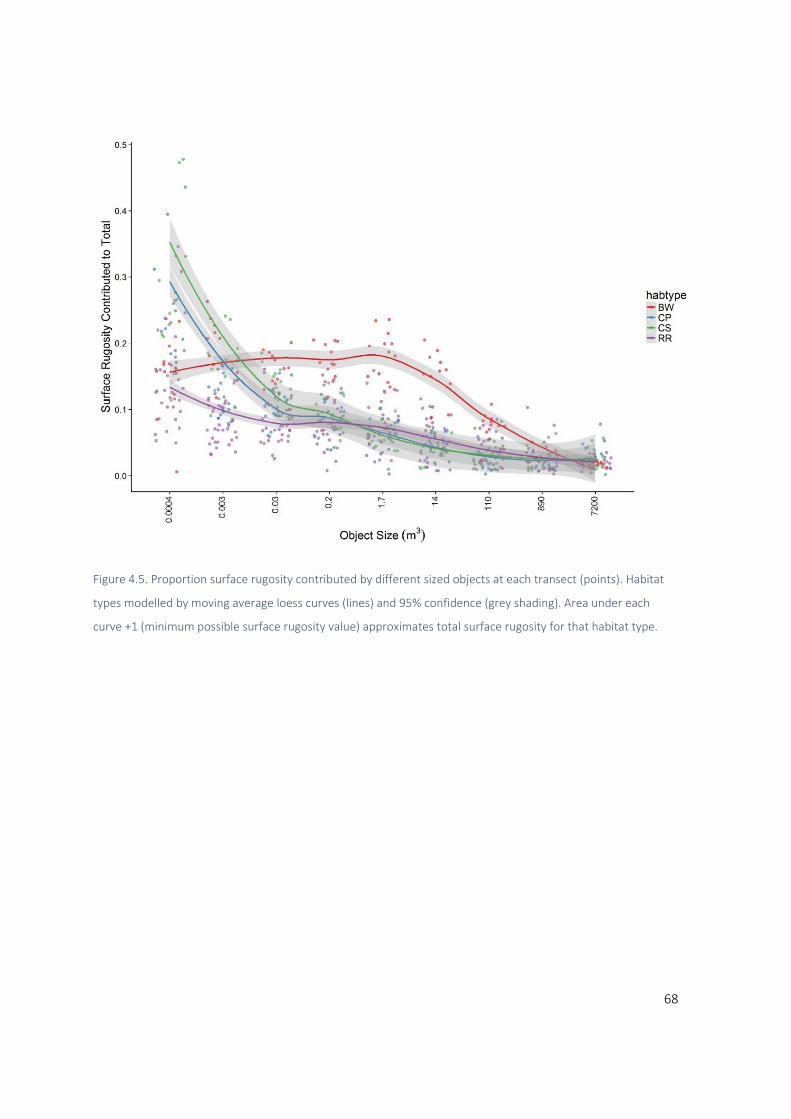
68  

 

Figure 4.5. Proportion surface rugosity contributed by different sized objects at each transect (points). Habitat 

types modelled by moving average loess curves (lines) and 95% confidence (grey shading). Area under each 

curve +1 (minimum possible surface rugosity value) approximates total surface rugosity for that habitat type. 

 

69  

 

Figure 4.6. Standardized surface rugosity contributed by different sized objects at each habitat type modelled by 

moving average loess curves with 95% confidence intervals in grey. Area under each curve approximates 1.  

 

70  

 

Figure 4.7. Boxplot of object size distributions by habitat type. Boxplots show median, first and third quartiles 

(box) range of data (points) and data within 1.5 inter quartile range of median (whiskers). Skewness of object 

size distributions (modes) are plotted on relative axes from distributions having more small objects to those 

having more large objects. Dashed grey line indicates significantly different groups (CS and CP have significantly 

more small objects than BW and RR). 

 

4.3.2C  Metric Composition 

There were significant differences in multivariate composition of structure metrics among habitat 

types (F = 20.47, df = 3, p = <0.001) (Figure 4.8). Habitats were significantly different for all pairwise 

comparisons except between the two coral habitats CS and CP, which were not significantly different 

(Table 4.4 and Figure 4.9). There were significant differences in mean dispersions among habitat types 

(F = 5.63, df = 3, p = 0.002). BW transects were significantly less dispersed than RR but none of the 

other pair‐wise comparisons were significant. 

 

71  

 

Figure 4.8. PCA plot of multivariate composition of all transects (points) based on all 6 structure metrics (black 

labels). Colour outlines indicate the multivariate space occupied by each habitat type (its characteristics). Grey 

vectors indicate increasing levels of each structure metric. 

 

Table 4.4. Multivariate pair‐wise ANOVA on structure composition among habitat types. P values are Bonferroni 

corrected for multiple comparisons and significant results indicate that habitats occupy a different multivariate 

space as defined by the 6 structure metrics measured. 

 Pair‐wise   F  p (adj) 

BW vs CP  38.92  0.006   * 

BW vs CS  36.49  0.006   * 

BW vs RR  37.92  0.006   * 

CS vs CP  1.84  0.82 

RR vs CP  8.96  0.006   * 

RR vs CS  14.79  0.006   * 

 

 

72  

 

Figure 4.9. Variability of habitat types as quantified by multivariate dispersion of transects. Boxplots show 

median, first and third quartiles (box) range of data (points) and data within 1.5 inter quartile range of median 

(whiskers). 

 

Multivariate visualization of object sizes by habitat types (Figure 4.10) displays clear trends with BW 

transects having high proportions of 1.7 and 0.2 m3 objects. RR habitat is notable for its variability, as 

well as having high proportions of the large 890 m3 size objects. CP and CS are characterized by high 

proportions of the smallest 0.0004 and 0.003 m3 size classes.  

 

73  

 

Figure 4.10. Multivariate visualization of differences among the composition of object sizes in m3 (grey overlay) 

at different habitat types (colours). Object sizes are standardized by total surface rugosity to allow comparisons 

of relative object size makeup of habitat types. 

 

4.4  Discussion 

In this chapter reef types are shown to differ significantly in structural character. Object size analysis 

captures important differences among reef types with coral habitats having more small features. 

Anthropogenic BW habitat have higher surface rugosity than the other habitats (at the resolutions 

captured here) but has less complexity from small objects. BW habitat is also more homogenous 

among transects than RR habitat and has more vertical surfaces and overhangs. 

Hypotheses about reef types differing in structure were supported with three groups emerging. BW 

and RR habitat consistently differentiated from other habitats while CS and CP remained similar to 

each other. There were some exceptions to these trends. BW and RR shared similar object size 

distributions, both having relatively larger objects than the coral habitats. RR also remained similar to 

the coral habitats in terms of slope and vertical relief. The fact that CP and CS remained similar in all 

the structural metrics calculated here implies that these metrics are sensitive to changes underlying 

broad habitat differences, but not to differences among habitats with similar sized objects. 

 

74  

Hypotheses about anthropogenic habitats being less variable were partially supported. When habitats 

were positioned in multivariate space, BW habitat occupied an almost entirely unique space, and was 

significantly less variable in structure than RR habitats. Chapter 2 of this thesis showed that β diversity 

at BW habitats is often low in comparison to rocky reefs. Homogeneity at large scales (i.e. among 

transects) is known to drive β diversity (Schneider et al. 1987) and is likely driving the trends observed 

in chapter 2 of this thesis. 

Hypotheses about object size distributions being different, and non‐linear were supported with three 

groups emerging. CS and CP, hereafter referred to as coral habitats, were not significantly different 

from each other, but had significantly higher abundance of small objects than BW and RR which were 

distinct from each other. The coral habitats mapped for this study generally had coral cover of at least 

40% (personal observation) and the underlying substratum and geomorphology of the area is 

dominated by coral processes (Harris et al. 2011). Therefore, the structural attributes of these 

transects were largely driven by the interaction of corals with external physical and ecological factors. 

Perhaps it is not surprising, therefore, that these landscapes display high abundance of small objects. 

But despite these data being intuitive, there have been very few successful attempts to quantify these 

patterns at ecologically meaningful extents and resolutions (10s of m2). In contrast to coral habitats, 

BW habitat showed a distinct peak in complexity contributed by the 1.7 m3 (refrigerator‐sized) 

category. This size of feature aligns with the roughly 1.5 metre protruding sides of the concrete 

hanbars, tetrapods and blocks used to construct BW (Blacka et al. 2005). Rocky reefs were quite 

variable in object size distributions (Figure 4.7).  

Object size distributions were significantly different among habitats, non‐linear and often unimodal. 

This has implications for the use of fractal dimension as a linear metric of complexity scaling. The 

method used in this chapter allows complexity to vary over the span of object sizes analysed, or 

spatial resolution, which it clearly does. Coral transects had 35% of their total complexity in the 

smallest object sizes while BW had a peak at medium object sizes. If fractal dimension is to be used as 

a metric of cross‐scale complexity, it should be calculated at numerous spatial resolutions to account 

for the non‐linear distribution of object sizes in marine habitats. 

Applying the TDH to these data, we would expect coral reefs to have significantly greater abundances 

of small fishes than BW, and especially RR habitat. This work would suggest that if elevated 

biodiversity on tropical reefs (Sale 1977) is being driven by some aspect of structural niche availability, 

it is likely an abundance of small sized features driving the pattern. Fishes are known to utilise physical 

 

75  

refugia corresponding to their body size (Luckhurst and Luckhurst 1978; Hixon and Beets 1993; 

Harborne et al. 2011; Harborne et al. 2012). Additionally, small bodied fishes have been shown to 

respond most to loss of small‐scale structure (i.e. corals) (Rogers et al. 2014). This has important 

implications for predicting biodiversity loss with climate change, as the complexity provided by coral 

habitat is projected to be highly impacted (Wernberg et al. 2013; Hughes et al. 2017). Understanding 

the implications of structural complexity for fish assemblages will be explored further in Chapter 5 of 

this thesis. 

This study was conducted at a defined spatial extent and resolution. Complexity across larger extents 

(i.e. embayments or seamounts) and smaller extents and resolutions (i.e. interstitial spaces in a coral 

colony) are also ecologically important. The object size curves at coral habitats show sharp increases 

at the smallest object sizes measured in this study (0.0004 m3 or approximately apple size). Even if 

coral habitats are not truly fractal, they certainly contain many objects smaller than an apple. 

Therefore, increasing the resolution of these 3D captured landscapes is likely to reveal more 

interesting patterns in habitat structural complexity of these landscapes, likely resulting in elevated 

surface rugosity values at coral habitats. Increasing the extent of these 3D captured landscapes would 

also likely yield other insights on cross‐scale ecological processes such as species richness (Peterson et 

al. 1998) or ecosystem resilience (Nash et al. 2015).  While increasing computational power will allow 

increases in resolution and spatial extent, the analysis conducted here represents some of the most 

thorough analysis of structure between and among habitat types to date. These measures of habitat 

structural complexity should provide fertile ground for exploration of fish/habitat relationships both 

within and among habitat types. 

 

76  

Chapter 5: Structural complexity drivers of reef fish assemblages: 

which metrics are important? 

 

Summary: 

1. Habitat structure is known to influence the distribution of organisms, but the specifics of this 

relationship are often lost in summary metrics. 

2. Here I test the relative importance of the structure metrics derived in Chapter 4 and their 

relationships with temperate fish assemblages, providing advice on which metrics should be 

captured to balance the trade‐off between cost of collection and ecological usefulness. 

3. Captured metrics explained between 8 and 61 % of variation in fish responses. Object sizes 

between 0.003 m3 and 1.7 m3 were consistently important and positively related to fish 

metrics.  

4. While overall complexity (as captured by surface rugosity) is important, the size of objects in a 

landscape appears to drive fish distribution on temperate reefs. 

5.1   Introduction 

Fish assemblages are known to respond to changes in physical habitat structure (Risk 1972; Luckhurst 

and Luckhurst 1978; Hixon and Beets 1989; Friedlander and Parrish 1998; Graham and Nash 2013). 

Relating fish assemblages to the structure of their habitats is important for numerous endeavours 

including fisheries management (Nash and Graham 2016), predicting climate change impacts (Wilson 

et al. 2006) and eco‐engineering (Strain et al. 2018). Historically, rugosity has been widely used to 

relate fish to HSC (Kovalenko et al. 2012). While ecologically predictive, rugosity is structurally non‐

explicit, limiting its usefulness as a design criterion (Loke et al. 2015). Recent advances in the digital 

capture of seascapes (Wedding et al. 2008; Zawada et al. 2010; Figueira et al. 2015) present an 

opportunity to analyse HSC in new ways ((Friedman et al. 2012; González‐Rivero et al. 2017) and 

Chapters 3 and 4 of this thesis). Emerging metrics derived from digitized seascapes are useful in 

predicting fish distribution (González‐Rivero et al. 2017; Ferrari et al. 2018). The wide variety of 

metrics calculated from digitized landscapes begs the question of which metrics are the most 

important predictors of biological assemblages such as fishes. 

 

77  

The habitat types tested in this chapter (breakwall and natural rocky reef) have different levels of 

structure metrics as detailed in Chapter 4 of this thesis. These metrics are likely to influence the 

distribution of fishes at these habitats (Chapter 1 of this thesis). There are, however, many aspects of 

habitat not captured by HSC that influence fish distribution. Assemblages of benthic and sessile 

organisms, for example, are known to influence fish distribution (Coleman and Connell 2001; Clynick 

et al. 2007; Trebilco et al. 2016). Like fish, benthic assemblages are also influenced by HSC (Loke et al. 

2017). Breakwalls have been shown to support different benthic assemblages than surrounding 

natural reefs (Airoldi et al. 2009; Burt et al. 2011; Dugan et al. 2011). It is possible that once HSC is 

thoroughly captured and explained, other elements of habitat will be un‐important in explaining fish 

distribution. Alternatively, there may be important aspects of breakwalls and natural reefs that are 

intrinsically different and not explained by metrics of HSC.  

The co‐linear nature of ecological predictor variables (Dormann et al. 2013), especially metrics of HSC 

(Ferrari et al. 2018) presents a significant barrier to developing an understanding of which metrics are 

most important to ecological response variables. The powerful and commonly used linear and additive 

modelling techniques are highly susceptible to over fitting and variance inflation in the presence of 

multi collinearity of predictor variables (Farrar and Glauber 1967; Dormann et al. 2013). The effort 

required to obtain and analyse these 3D captured seascapes is not trivial (author’s personal 

observation). Optimising data collection should, therefore, be a priority. One statistical method that is 

capable of discerning relationships between responses and multiple, co‐linear predictor variables is 

random forest (RF) analysis (Breiman 2001). This method is based on many boosted regression trees 

(Schapire et al. 1998) and implements an ensemble learning algorithm (Breiman 2001) to determine 

the effect and relative importance of each predictor variable. By calculating the effects of randomly 

permuted subsets of predictors at each node of every tree, relationships are modelled, and relative 

importance of variable is determined. This method does not assume linear relationships between 

dependent and independent variables. 

There is a gap in knowledge around what metrics are most important to different fish groups, and 

what metrics should be captured. This chapter will compare the suite of metrics from Chapters 3 and 

4 to fish assemblage data from some of the transects described in chapter 2 to determine which 

metrics are important in explaining the distribution of fishes at temperate reefs. 

 

78  

Aims 

1. Determine the level of correlation among predictor variables and object sizes in a landscape. 

2. Compare the relative importance of complexity metrics for explaining variance in fish species and functional groups. 

3. Determine if habitat type remains important even when structure metrics are explained. 

5.2   Methods 

This study related temperate reef fish assemblages to metrics of habitat structural complexity to 

determine which metrics are most useful in explaining habitat‐fish relationships. Fish were counted by 

underwater visual census over 25 m long and 10 m wide transects following the Reef Life Survey 

Methodology (Edgar and Stuart‐Smith 2014), as described in Chapter 2. The terrain in each transect 

was mapped in 3D using the methods described in Figueira et al. (2015). The 3D maps were analysed 

for the metrics of habitat structural complexity detailed in Chapter 3 of this thesis. Due to the 

expected co‐linearity of metrics of structure, standard modelling techniques were not appropriate. 

Therefore, random forest analysis (RF) (Breiman 2001; Liaw and Wiener 2002) was conducted in R v 

3.4.0 to determine the relative importance of the structure metrics in explaining observed variance in 

14 different aspects of fish assemblages. Each of these methodologies is described in greater detail 

below. 

5.2.1  Study Design 

Fish census and 3D structure capture was carried out at 46 transects from a total of 8 sites in two 

regions: Botany Bay and Port Kembla. Each region included 4 sites, one at breakwall habitat and 3 

control sites at rocky reef habitat. Each site had 6 transects. The 3D capture process failed at one 

control transect at each of the regions, resulting in a total n of 46 transects. All transects were at rocky 

reef (either natural or anthropogenic breakwall) with interspersed sand patches and kelp. Transects in 

this chapter are the same as those at Botany Bay and Port Kembla in Chapters 2 and 4 of this thesis. 

Transects were selected to control for depth, reef size and exposure. See Chapter 2 of this thesis for 

full details on sites and transects. This study is designed to quantify the relative influence of structural 

features on fish assemblages, and to determine if they explain differences between breakwall and 

natural reef habitats. The factors of habitat type and region are known to be important (see chapter 

2). This chapter focuses on the underlying structural causes for observed differences. Therefore, 

transects were pooled and compared among sites and habitats. 

 

79  

5.2.2  Habitat Structural Complexity (predictor) Data 

Transect were mapped and reconstructed using the photogrammetry software Agisoft Photoscan Pro 

(v1.3.0‐1.3.3) following Figueira et al. (2015) (see chapter 4 of this thesis for details). Each mesh was 

scaled using a minimum of 2 features of known size and oriented to real‐world up (z coordinate) using 

mid water buoys deployed at the sites. Each transect was expressed as a 3D mesh of approximately 

8,000 triangles per m2 yielding resolutions (distance between vertices) of approximately 3 cm. Areas 

of obviously bad mesh and any visually apparent edge effects were removed. Holes smaller than 2 

metres at their widest point were filled with flat mesh using the CAD software Geomagic Control 

(v2015.1.1). Meshes were then analysed for metrics of structure described in Table 5.1 following the 

methods described in Chapter 3 of this thesis. 

 

80  

Table 5.1. Metrics of structural complexity and descriptions of how they are calculated. For further details see 

Chapter 3 Appendix on complexity metrics software and Chapter 3 of this thesis. 

Metric Abbreviation  Metric  Calculated as 

sr_pbf  Surface Rugosity (plane of best fit) 

The ratio of the total surface area over the planar extent covered (the shadow cast). Calculated on the plane of best fit to the whole transect. This metric includes information on the mean slope of each transect.

sr_xy  Surface Rugosity (horizontal xy plane) 

The ratio of the total surface area over the planar extent covered (the shadow cast). Calculated on the xy (horizontal plane. This metric is a measure of the surface roughness which is not independent of broader landscape slope. 

oh  Overhang  Sum of all surface area in each transect with face angle > 90 deg (area beyond vertical). 

slope  Landscape slope  Mean slope of each transect. 

relief  Vertical relief  Highest (shallowest) point on each transect minus the lowest (deepest) point.  

steep  Face angle (steepness) 

Right skewness of face angle distribution. Larger numbers indicate habitat with proportionally more surface area of steep faces.

os_lrg  Skewness of object size distribution towards large objects

Degree of right skew of object size distribution. Larger numbers indicate habitat with proportionally more large objects. 

os_###  Object Sizes  Complexity contributed by 9 individual object size categories. Note that objects include both protrusions of the specified size, and depressions of that size. Each category encompasses a range of sizes, centred on the size listed. Object sizes in m3 and roughly equivalent sized real‐world objects: 0.0004 m3 = apple size 0.003 m3 = soccer ball size 0.03 m3 = suitcase size 0.2 m3 = washing machine size 1.7 m3 = refrigerator size 14 m3 = van size 110 m3 = shipping container size 890 m3 = house size 7200 m3 = airplane hangar size 

 

5.2.3   Fish (response) Data 

Fish were identified to species level and their length visually estimated by teams of two trained divers 

at each transect (as per standard Reef Life Survey methodology) (Edgar and Stuart‐Smith 2014). 

 

81  

Length categories of 2.5, 5, 7.5, 10, 20, 35, 50+ cm. were used to calculate biomass based on 

established length to weight ratios (Duffy et al. 2016). Fish were also categorised into functional 

groups based on the taxon’s recorded water column position and trophic group using information 

from Fishbase.com and a published field guide (Kuiter 1993). Highly mobile coastal pelagic species 

were excluded from analyses as they were not well quantified at the scale of this study. See chapter 2 

of this thesis for full fish survey method details. 

β diversity of fish species at each site was calculated among transects at a site using Jaccard’s index 

(Jaccard 1900a) and the package betapart (Baselga and Orme 2012). This resulted in a β diversity 

value for each site (a linear stretch of habitat at least 200 m long). Jaccard’s index was chosen because 

it is directly interpretable as the percent of unshared species among transects at a site. Because β 

diversity operates at the scale of multiple transects in a site, the above predictor variables (which 

summarize complexity of individual transects) were not expected to drive β diversity within sites. 

Instead, the coefficient of variation (CV) of each predictor variable amongst transects within a site was 

calculated. These data were used as predictors of β diversity in analyses. 

Table 5.2. Metrics of fish assemblages and descriptions of each. See Chapter 2 of this thesis for further details on 

capture and calculation of each metric. All metrics are calculated per transect. 

Fish Metrics Metric  Description 

Total abundance  The total number of individual fishes observed.

Biomass  The total weight of individuals as calculated by estimated length of each individual and established length to weight ratios for each species. 

# large fishes   The number of individual fishes weighing more than 200 g. 

# midsize fishes  The number of individual fishes between 20 g and 200 g. 

# small fishes  The number of individual fishes weighing less than 20 g. 

Shannon diversity (H)  Richness corrected for evenness.

β Diversity   Species turnover among transects. Calculated as Jaccard Index and interpretable as % unshared species between transects. 

Species richness  The number of species present.

Functional richness  The number of distinct functional groups present (see functional groups below) 

Functional groups  Each species was allocated to one of three water column positions (benthic, demersal or midwater) and one of five trophic groups (herbivore, planktivore, infauna‐predator, meso‐predator or piscivore). The combination of water column position and trophic group resulted in 15 distinct functional groups. 

 

 

82  

5.2.4   Statistical analysis 

To test the level of correlation among habitat structural complexity metrics, all pairwise comparisons 

plotted in a correlation plot. To test the relative importance of metrics of habitat structural complexity 

in explaining fish responses, all structure metrics were compared to each fish response. Due to the 

expected co‐linear nature of structure metrics, however, normal linear and additive modelling 

techniques were not appropriate as they are sensitive to collinearity of predictor variables (Farrar and 

Glauber 1967). A different approach was required. Random forests (RFs) are a class of supervised 

machine learning algorithm based on bootstrap aggregated regression trees. By considering a random 

subset of predictor variables at each node of each tree, and comparing the results of all trees, multi‐

collinearity is accounted for. This method enables assessment of relative importance of predictor 

variables even when they are highly correlated (Cutler et al. 2007).  

The r package randomForest (Liaw and Wiener 2002) was used to determine the relative importance 

of structure metrics to fish responses. A separate RF model was fit for each fish responses metric as a 

function of all 17 predictor variables (fixed factors) following the same procedure. Bagging (Breiman 

1996) was used to identify the optimal number of variables to consider at each node. Then the RF 

model was fit using 9000 permutations of regression trees. Predictor (structure) variables were 

ranked by importance based on % incremental MSE which is a measure of how much each variable 

contributes to the splitting at each node of all regression trees in the forest. The relationship of each 

fish response to all structure metrics was visualized based on relative importance of the structure 

metrics using scaled (as each metric has a different max value) % incremental MSE values. The three 

most important structure variables for each fish response were further visualised with partial 

dependence plots using the package plotmo (Milborrow 2015). Partial dependence plots display the 

relationship between a predictor variable (structure) and response variable (fish) once the effect of 

the other predictors has been accounted for by the RF analysis. 

To verify that this analysis is robust to multi‐collinearity, a model was run using the methods described 

above, but excluding habitat type as a variable (see Appendix 5.3). 

5.3   Results 

5.3.1  Predictor Variables 

Surface rugosity horizontal (sr_xy) and surface rugosity plane of best fit (sr_pbf) were 99.05% 

correlated (Figure 5.1). Sr_xy was more closely correlated with other structural metrics, especially 

 

83  

slope and overhangs, and was therefore dropped from further exploration. Different metrics of 

structure were up to 97% correlated. The established metrics (surface rugosity xy, overhang, slope 

and relief) were between 76% and 95% correlated to each other. Object sizes between os_0.003 and 

os_14 were also highly correlated with standard metrics of complexity (between 70% and 96%). 

Os_0.0004 and the large (os_890 and os_7200) sized objects were less than 40% correlated to all 

other metrics of structure. 

 

Figure 5.1. Correlation table of the 16 metrics of structure, including 9 object size categories. Blue numbers are 

positively correlated, red negatively correlated. Numbers in each cell are R2 values. 

 

5.3.2  Random Forest results 

5.3.2A  Assemblage summary metrics 

When considering the overall assemblage summary metrics, between 8% and 60% of variation was 

explained by the 15 structure metrics. Object sizes between os_0.03 and os_1.7 were consistently 

among the most important metrics (Figure 5.2 and Figure 5.3). Slope, os_lrg, os_0.0004 and os_7200 

 

84  

were not important predictors of any fish responses. Habitat type was highly important to richness, 

diversity and medium sized fishes, all of which were higher at BW habitat. Sr_pbf was positively 

associated with all fish responses, but not among the most important metrics. Most metrics of 

structure were positively correlated with fish responses, although a few instances of important 

negative relationships did occur with diversity and β diversity, although relatively little variance was 

explained in these metrics (Figure 5.4). 

Models including and excluding habitat type showed only minimal differences in correlations between 

fish and structural metrics (Appendix 5.3). Models including habitat type are presented here. 

 

85  

 

Figure 5.2. Partial dependence plots of the three most important predictor variables (in columns) for each fish 

assemblage summary metric (in rows). These plots display the relationship between the dependent variable (the 

aspect of fish assemblages, y axes) and the independent variables (structure metric noted above each plot, x 

axes) as determined by random forest analysis. The relationships are observed data and not predictions. 

 

86  

 

Figure 5.3. Partial dependence plots of the three most important predictor variables (in columns) for each fish 

size class (in rows). These plots display the relationship between the dependent variable (the aspect of fish 

assemblages, y axes) and the independent variables (structure metric noted above each plot, x axes) as 

determined by random forest analysis. The relationships are observed data and not predictions. 

 

Abundance and biomass showed similar patterns with 60% and 55% of variation explained 

respectively and both highly responsive to os_0.03. Species richness was most responsive to habitat 

type and os_0.03 with a total of 39% of variation explained. Habitat type was also the most important 

predictor of diversity with a total of 13% of variation explained. Vertical relief was also important in 

explaining changes in diversity, with more relief associated with lower diversity. The most important 

metric for the number of large fishes was os_110, with overhang and steep surfaces also important 

and a total of 17% of variation explained. Medium fish had 43% of variation explained and were 

responsive to habitat type, steep surfaces, os_1.7 and os_14. For small fish, in contrast, os_0.2 stood 

 

87  

out as the one important metric. β diversity was responsive to variation in os_0.2 and os_1.7 and 8% 

of variation was explained. Partial dependence plots of the 3 most important predictors for each fish 

response illustrated the relationships. Non‐linear relationships were apparent for many of the 

relationships, including apparent thresholds at which response variables responded strongly. 

 

Figure 5.4. Direction and relative importance (as determined by random forest analysis) of relationships 

between predictor variables (columns) and fish responses (rows) based on standardised % incremental MSE. 

Green indicates a positive relationship, red a negative relationship, and the intensity of the colour denotes the 

importance of each variable (darker being more important). 

 

5.3.2B  Functional groups 

Of the 15 possible combinations of trophic group and water column position, 12 were detected in our 

data and 5 were detected consistently enough to analyse with the random forest method (i.e. 

occurring in at least 15 transects). They were midwater piscivores, midwater planktivores, demersal 

herbivores, demersal planktivores and demersal predators. Small os_0.003 objects were the most 

important single metric to these functional groups in general (Figure 5.5). Habitat type and sr_pbf 

were only marginally important for functional groups. Slope, os_lrg, os_0.0004, os_890 and os_7200 

were not important predictors of any functional groups.  

 

88  

 

Figure 5.5. Partial dependence plots of the three most important predictor variables (in columns) for each of the 

functional group fish responses (in rows). These plots display the relationship between the dependent variable 

(the aspect of fish assemblages, y axes) and the independent variables (structure metric noted above each plot, 

x axes) as determined by random forest analysis. The relationships are observed data and not predictions. 

 

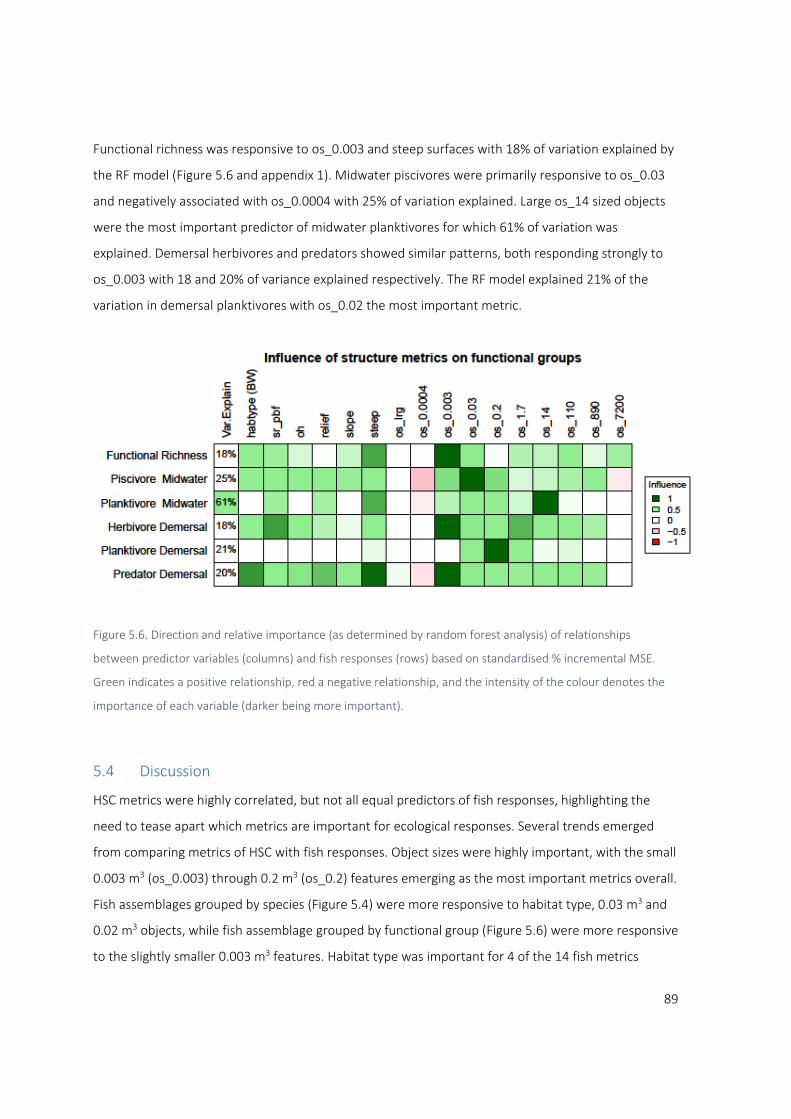
89  

Functional richness was responsive to os_0.003 and steep surfaces with 18% of variation explained by 

the RF model (Figure 5.6 and appendix 1). Midwater piscivores were primarily responsive to os_0.03 

and negatively associated with os_0.0004 with 25% of variation explained. Large os_14 sized objects 

were the most important predictor of midwater planktivores for which 61% of variation was 

explained. Demersal herbivores and predators showed similar patterns, both responding strongly to 

os_0.003 with 18 and 20% of variance explained respectively. The RF model explained 21% of the 

variation in demersal planktivores with os_0.02 the most important metric. 

 

Figure 5.6. Direction and relative importance (as determined by random forest analysis) of relationships 

between predictor variables (columns) and fish responses (rows) based on standardised % incremental MSE. 

Green indicates a positive relationship, red a negative relationship, and the intensity of the colour denotes the 

importance of each variable (darker being more important). 

 

5.4   Discussion 

HSC metrics were highly correlated, but not all equal predictors of fish responses, highlighting the 

need to tease apart which metrics are important for ecological responses. Several trends emerged 

from comparing metrics of HSC with fish responses. Object sizes were highly important, with the small 

0.003 m3 (os_0.003) through 0.2 m3 (os_0.2) features emerging as the most important metrics overall. 

Fish assemblages grouped by species (Figure 5.4) were more responsive to habitat type, 0.03 m3 and 

0.02 m3 objects, while fish assemblage grouped by functional group (Figure 5.6) were more responsive 

to the slightly smaller 0.003 m3 features. Habitat type was important for 4 of the 14 fish metrics 

 

90  

calculated, with increases of each metric at breakwall habitat. Figure 5.4 and Figure 5.6 highlight the 

generally positive relationship between all metrics of HSC and all metrics of fish measured here. The 

primary exception to this generalization was the sharp decline in species diversity at about 4 m of 

vertical relief. This pattern is likely driven by increases in one highly abundant midwater planktivore 

species reducing evenness, and therefore Shannon diversity (Figure 5.6).  

Non‐linear relationships between structure and fish were quite prevalent (Figure 5.2, Figure 5.3 and 

Figure 5.5). Many of the most important relationships appear to be thresholds, above which fish 

groups increase sharply. Objects in the 0.03 m3 size range, for example, was a consistently important 

predictor that appeared to have a threshold effect. Fish abundance, species richness, species 

diversity, biomass, midwater planktivores and demersal planktivores all displayed marked increases 

when roughly 10‐15% of the complexity in a habitat was contributed by 0.03 m3 objects. Midwater 

piscivores also showed a threshold response to 0.03 m3 objects but this group appeared to require 

closer to 20% of the complexity to consist of this object size. The slightly smaller 0.003 m3 objects also 

drove threshold responses in fish groups. Species richness, functional richness, demersal predators 

and demersal herbivores all increased markedly when at least 12‐15% of the complexity was created 

by 0.003 m3 objects.  

There were some notable instances of high percent variance in a fish group explained by a single HSC 

metric. Midwater planktivores showed a striking positive association with large 14 m3 objects. This 

finding aligns with behavioural knowledge of this functional group utilising turbulence and upwelling 

from large vertical structures for feeding and schooling behaviour to mitigate predation (Kuiter 1993; 

Champion et al. 2015; Morris et al. 2018). Biomass increased sharply when at least 10% of the 

complexity in a habitat was created by 0.03 m3 objects. Abundance also responded strongly to 0.03 m3 

objects, as well as 0.2 m3 objects. The response of both biomass and abundance likely indicates a 

broad‐based increase in many fish groups associated this object size. 

Surface rugosity (Sr_pbf) was a relatively un important predictor of the fish groups analysed here. 

Rugosity was, however, positively correlated with all but one of the fish responses. This evidence does 

not conflict with the species area relationship (Preston 1962), but it does suggest that other ecological 

processes may be more important in driving fish distribution. Habitat type (breakwall or natural rocky 

reef) was important for 4 of the fish responses measured in this study. Breakwall habitat was the 

single most important predictor of increases in three fish metrics; species richness, species diversity 

and medium sized fishes. Abundance of demersal predators was also weakly associated with 

 

91  

breakwall habitat. This relationship points to edge effects related to the breakwalls in this study being 

entirely surrounded by sand. While the rocky reefs in this study were also surrounded by sand, they 

were often larger. Smaller reef size has been linked to increased abundance and diversity of fish 

(Bohnsack et al. 1994). Ecotones (the meeting of two habitats such as sand and rock) also drive 

changes in assemblages, especially ecotone specialists like many demersal predators (Bellquist et al. 

2008). 

Chapter 2 of this thesis documented increases in fish at breakwalls but did not include rigorous 

analysis of HSC metrics. The data presented in this chapter indicate that breakwall habitat drives some 

aspects of fish distribution even when the structural complexity of the habitat is rigorously quantified. 

This suggests that either breakwalls coincidentally have a mix of habitat features that are particularly 

attractive to fish, or that there is another component of the habitat driving increases in these fish 

metrics at breakwalls. Benthic assemblages differ between natural and artificial substrates with 

breakwalls often supporting less diverse benthic assemblages than adjacent natural reefs (Moschella 

et al. 2005; Dugan et al. 2011). It is, however, unclear how less diverse benthic assemblages would 

drive increased diversity of fishes. Chapter of this thesis 2 also found decreased β diversity at 

breakwall habitat. The results presented here do not provide strong support for this theory, with only 

a small amount of variance in β diversity explained by variance in complexity metrics. 

In the context of the textural discontinuity hypothesis (Holling 1992), object sizes would be expected 

to drive corresponding body size categories of resident animals. The data in this chapter present some 

evidenced for this relationship, although at larger scale than expected. Object sizes of 0.2 m3, 1.7 m3 

and 110 m3 were the most important object sizes for small (<20 g), medium (20 g – 200 g) and large 

(>200 g) fishes respectively. While shelter size – body size mechanistic relationships were anticipated 

(Hixon and Beets 1989), 1.7m3 refugia are larger than expected to provide shelters for 20g – 200g 

fishes. These results suggest that other mechanisms are likely at play in determining the relationships 

between body size and refuge size. 

Many of these findings translate directly to design advice for the construction of temperate fish 

habitat. If abundant and high biomass assemblages are a desirable outcome, at least 10 ‐15% of the 

complexity should be created by objects in the 0.03 m3 size range. If midwater planktivores (often 

valued as bait and attractants for highly desirable recreationally fished species (Kuiter 1993; Griffiths 

2012)) are desirable, large features in the 14 m3 size range should be included in reef habitat designs. 

Interestingly, overall surface rugosity, very small (0.0004 m3) features and very large (890 m3) features 

 

92  

do not appear to be important to fish assemblages at temperate reefs. Object size analysis is useful 

both as design criteria for habitat creation, and for testing underlying theories of habitat use. These 

findings underscore the utility of structurally explicit metrics of HSC. As digital capture of landscapes 

expands to more environments developing ways to use this data will be critical to advancing 

ecological knowledge. 

 

 

93  

Chapter 6: General discussion 

6.1 Summary of research and findings 

The structural complexity of habitats is linked to maintenance of abundant and diverse ecosystems 

(MacArthur and MacArthur 1961; Hixon and Beets 1993; Knudby et al. 2010; Harborne et al. 2011; 

Harborne et al. 2012; Graham and Nash 2013; Malcolm et al. 2014). This abundance and richness are 

under threat as anthropogenic changes to habitat structural complexity such as urbanisation, 

destructive fishing methods and climate change are likely to increase in the future (Wernberg et al. 

2013; Bozec et al. 2015; Hughes et al. 2017). Understanding the implications of these changes and 

actively using this knowledge to create habitat will determine how much biodiversity is retained 

through the Anthropocene (Wernberg et al. 2012). The work presented in this thesis aimed to 

improve the mechanistic understanding of fish responses to structure, both natural and man‐made, 

providing advice for the creation of future habitat. 

Chapter 2 of the thesis established a baseline of fish assemblages at categorical habitat types without 

analysis of habitat structure (Figure 6.7). The results revealed a mixed picture of some significant 

differences between natural rocky reefs and anthropogenic breakwalls. Breakwalls supported 

desirable, rich and abundant assemblages. But the perceived landscape scale homogeneity of these 

habitats was suggested as a driver of the low β diversity of resident taxa. Chapter 3 of this thesis 

created and validated novel metrics of structural complexity for ecologically relevant analysis of digital 

landscapes. The new metrics, as well as several commonly used metrics were trialled using digital 

landscapes of known proportions. Equations and algorithms presented here allow detailed analysis of 

object sizes in a landscape. This represents an important step beyond structurally non‐explicit metrics 

of complexity and links theory, mapping and habitat creation. Chapter 4 of the thesis analyses the 

structural character of different reef habitat types (coral slopes, coral patches, breakwalls and rocky 

reef) using the metrics detailed in Chapter 3. Coral slopes and coral patches shared similar structural 

attributes with high abundance of small structural features. Breakwalls had high surface rugosity but 

few small features. Natural reefs had relatively even distributions of feature sizes and low surface 

rugosity. Chapter 5 linked structural attributes to fish distribution, showing that fish generally respond 

positively to structure, but that certain aspects of structure are exceptionally important. Habitat type 

was important to 4 of the 14 fish responses indicating that there are important aspects of habitat not 

explained by physical structure. Objects in the 0.03 m3 size range were the most important structural 

 

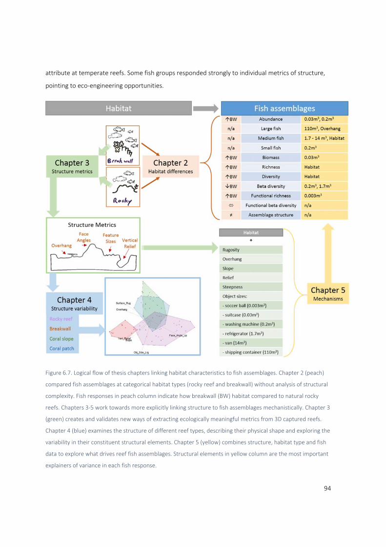
94  

attribute at temperate reefs. Some fish groups responded strongly to individual metrics of structure, 

pointing to eco‐engineering opportunities.  

 

Figure 6.7. Logical flow of thesis chapters linking habitat characteristics to fish assemblages. Chapter 2 (peach) 

compared fish assemblages at categorical habitat types (rocky reef and breakwall) without analysis of structural 

complexity. Fish responses in peach column indicate how breakwall (BW) habitat compared to natural rocky 

reefs. Chapters 3‐5 work towards more explicitly linking structure to fish assemblages mechanistically. Chapter 3 

(green) creates and validates new ways of extracting ecologically meaningful metrics from 3D captured reefs. 

Chapter 4 (blue) examines the structure of different reef types, describing their physical shape and exploring the 

variability in their constituent structural elements. Chapter 5 (yellow) combines structure, habitat type and fish 

data to explore what drives reef fish assemblages. Structural elements in yellow column are the most important 

explainers of variance in each fish response. 

 

95  

 

6.2  Fish responses to structure 

6.2.1  The importance of object size distributions   

Structurally explicit and cross‐scale measures of complexity unlock ecologically important information 

for testing ecological theory, measuring ecological responses and informing habitat creation. The 

complexity of a habitat has long been understood to facilitate abundance and diversity, but the 

studies presented here show that the size of structural features, not just the overall complexity, is a 

highly important aspect of temperate reef habitat. While surface rugosity was consistently positively 

associated with fish responses, it was not among the most important metrics of HSC. Reef structural 

features in the 0.03 m3 range were the most important single metric to fish assemblages of the 14 

HSC metrics examined in the thesis (Figure 6.8). Specific groups of fishes showed strong associations 

with features ranging from 0.003 m3 to 110 m3, highlighting the utility of viewing structure through 

the object‐size lens. The midwater planktivore group of fishes showed a striking association with 

features in the 14 m3 size range. This fits with the ecology of this group utilizing tall structures for 

feeding (Kuiter 1993; Champion et al. 2015; Morris et al. 2018). The underlying drivers of fish 

associations with other feature sizes are not well studied in temperate reef habitats, pointing to a 

knowledge gap for future study. Why high abundance, piscivores and species richness were associated 

with 0.03 m3 objects, for example, is not known.  Large numbers of bullseyes (Pempheridae spp.) were 

observed sheltering among overhanging features in the 0.03 to 0.2 m3 size range at both rocky reef 

and breakwall habitats. It is possible that small schooling species utilise this sized feature for shelter, 

attracting increased midwater piscivores and elevating overall abundance. Roberts and Ormond 

(1987) found that holes of sizes equivalent to 0.03 and 0.2 features in this thesis were associated with 

high abundance of coral reef fishes, although this relationship does not appear to hold true for fishes 

at mangrove and seagrass habitats (Gratwicke and Speight 2005b). This disparity in fish responses to 

structure points to the importance of testing the conclusions of this thesis in other habitats (see 

section 6.5.1 below).  

 

96  

 

Figure 6.8. Reproduction of figure 5.4 and 5.6 in chapter 5. Direction and relative importance (as determined by 

random forest analysis) of relationships between predictor variables (columns) and fish responses (rows) based 

on standardised % incremental MSE. Green indicates a positive relationship, red a negative relationship, and the 

intensity of the colour denotes the importance of each variable (darker being more important). 

 

6.2.2  Textural Discontinuity 

Ecosystems are shaped by trophic, biotic and physical interactions operating at multiple scales 

(MacArthur and MacArthur 1961; Peterson et al. 1998). Structures such as coralline algae or kelp that 

    

 

97  

create complexity at one scale may not create complexity at other scales (Kelaher 2003; Trebilco et al. 

2015), leading to discontinuities in cross‐scale complexity. The results presented here provide strong 

support for the prediction of the textural discontinuity hypothesis (TDH) (Holling 1992) that physical 

structure and refugia are not evenly distributed across scales. Textural discontinuity was empirically 

observed with object sizes not evenly distributed across scales (Figure 6.9). Peaks in complexity were 

observed at expected object sizes. Coral reefs, being dominated by the coral keystone structures 

(Tews et al. 2004), showed extreme peaks at the smallest object sizes measured. Rocky reefs had the 

most even distribution of feature sizes and breakwalls were dominated by features in the 1.7 m3 

(hanbar‐size) range (Blacka et al. 2005). The TDH also predicts that the body sizes of animals 

occupying a habitat will be “entrained” to fit the available refugia. This thesis found evidence 

supporting the entrainment prediction, with increasing sized fishes associated with increasing sized 

objects, although the object sizes were larger than expected. Large (>200 g) fishes associated with 110 

m3 (roughly shipping container sized) objects. Medium fishes associated with 1.7 m3 objects and small 

(<20 g) fishes associated with 0.2 m3 objects. Herbivores at coral reefs show body size‐specific 

“entrainment”, responding to refuges according to their body size (Nash et al. 2013). The smallest 

refugia measured by Nash et al. were roughly 0.00003 m3 (an order of magnitude smaller than the 

smallest objects measured in this thesis). In this thesis herbivores responded most strongly to much 

larger 0.003 m3 objects pointing to trophic latitudinal and/or habitat type dependent relationships. It 

is also possible that trophic interactions cause indirect responses. Large fish, for example could be 

expected to respond to increased numbers of small fish that they may predate on. The data presented 

here do not, however, support these mechanisms as large fish and small fish appear to be responding 

to different structural features, as do piscivores and planktivores. 

 

98  

 

Figure 6.9. Reproduction of figure 4.5 from chapter 4. Proportion surface rugosity contributed by different sized 

objects at each transect (points). Habitat types modelled by moving average loess curves (lines) and 95% 

confidence (grey shading). Area under each curve +1 (minimum possible surface rugosity value) approximates 

total surface rugosity for that habitat type. 

 

6.3 Anthropogenic habitats and remediation 

6.3.1  Fish responses to anthropogenic habitat 

Anthropogenic habitats can have strong effects on marine biota (Bulleri and Chapman 2004; Clynick et 

al. 2008; Burt et al. 2013). This pattern was observed at the breakwalls and natural reef comparisons 

made in the chapters of this thesis. Importantly, the work in the above chapters provides critical 

insights into the underlying drivers of these patterns. Chapter 2 showed that breakwalls support 

desirable assemblages of fish characterized by high abundance and biomass of native species without 

loss of functional groups. Species richness at the transect scale (25 m) was also high at breakwater 

habitat. At the landscape scale, β diversity was low at breakwall habitats, indicating that the 

homogeneity of anthropogenic structures may play a role in reducing their ecological value (Shmida 

 

99  

and Wilson 1985). Landscape scale complexity is known to drive β diversity (Schneider et al. 1987) and 

this pattern holds true for sessile assemblages at breakwaters (Aguilera et al. 2014). Chapter 5 of this 

thesis found weak positive relationships between habitat structural heterogeneity (variance of 0.2 and 

1.7 m3 objects) and β diversity. Chapter 2 of this thesis is, to my knowledge, the first study of β 

diversity of mobile organisms at breakwalls and the results translate directly to design advice. Where 

possible, marine infrastructure should include habitat heterogeneity at extents greater than 25 m to 

increase β diversity of mobile organisms and therefore ecological value at the landscape scale.  

The work presented in the above chapters confirms that there are important aspects of habitat not 

captured by HSC metrics. Habitat type remained an important predictor of some fish responses after 

the HSC of breakwalls and rocky reefs was accounted for (Chapter 5). Species richness, diversity and 

the number of 20 – 200 g fishes all responded strongly to habitat type, increasing at breakwall 

habitats (Figure 6.8). The assemblage of sessile and benthic organisms is one factor that is likely 

influencing fish distribution, but not reflected in the HSC metrics used here. Benthic organisms are an 

important driver of fish distribution (Clynick et al. 2007) and artificial substrates drive changes in 

benthic assemblages (Bulleri and Chapman 2004; Dafforn et al. 2012; Perkol‐Finkel et al. 2012). 

Incorporating information on benthic organisms into analyses like those in this thesis would likely 

result in greater explanatory power (Harborne et al. 2011; Ferrari et al. 2018).  

6.3.2  Habitat creation and remediation  

The question of how to remediate marine systems when natural structures are lost to development, 

or more optimally, how to better design such structures in the first place, is ever more pressing. The 

studies in the above chapters provide directly actionable guidance for the creation or remediation of 

temperate reef habitat. The findings from chapter 2 highlight the importance of multi‐scale 

heterogeneity for β diversity. Designed reefs, including breakwalls, should include landscape‐scale 

variability at 25 m+ scales. The findings from Chapter 5 also provide design advice for building reef 

habitat. Features in the 0.003 m3 – 0.03 m3 size range (roughly soccer ball to suitcase size) are highly 

important to temperate fish assemblages. Partial dependence plots showed that reefs should include 

at least 15% of their complexity from features in this size range to facilitate abundant, high biomass, 

rich and functionally rich fish assemblages. Larger structures in the 14 m3 to 110 m3 size range 

(roughly van size to shipping container size) were important to the socially and economically valuable 

large fish and midwater planktivorous fish categories (Kuiter 1993). Partial dependence plots indicated 

that roughly 10% of the complexity should be constructed of these larger features. For planktivores, 

 

100  

the height of these large features may be more important than their volume (Morris et al. 2018; Strain 

et al. 2018). These findings highlight the utility of structurally explicit analysis of HSC developed in this 

thesis. In the context of eco‐engineering and climate change HSC remains one of the most easily 

changed aspects of a habitat in the pursuit of augmenting ecological outcomes (Dafforn et al. 2015; 

Loke et al. 2015; Mayer‐Pinto et al. 2017). Building the required ecological knowledge to create 

mechanistic links between built structure and ecological responses is fundamental to this endeavour. 

The approaches and information in this thesis contribute to this effort. 

6.4  Measuring structural complexity 

It is clear that structural complexity is often one of the most important factors driving the distribution 

and abundance of organisms. The work of this thesis has highlighted that importance can, in some 

cases, even supersede that of the general type of habitat involved. But this thesis has also highlighted 

the significant explanatory power of ecologically relevant measures of structural complexity derived at 

high resolution and over large areas. This then raises the challenge of how to most effectively gather 

and analyse data on the structural complexity of reefs. Monitoring programmes are increasingly using 

stereo video to examine fish‐habitat associations (Collins et al. 2017). Managers will need to examine 

the costs and benefits of conducting 3D capture approaches vs stereo video. Alternately, 

opportunities to combine the two techniques would provide exciting datasets. 

This thesis presented methods and metrics that capture structurally explicit and ecologically 

important aspects of HSC at fish‐relevant extent and resolution. Object sizes were derived from 3D 

landscapes, marking a drastic improvement in the applicability of cross‐scale structure to habitat 

creation. Fishes interact with their habitat at both fine resolution and broad scale. Ecologists have 

long known that measuring processes at appropriate extent and resolution is both critically important 

(Holling 1992; Peterson et al. 1998; Frost et al. 2005) and difficult (McCoy and Bell 1991; Kovalenko et 

al. 2012). The fractal dimension has been used to describe the scaling properties of complexity in a 

landscape (Mandelbrot 1982; Frost et al. 2005; Zawada and Brock 2009). While this method is 

ingenious and aesthetically appealing, it assumes a linear relationship between resolution and 

complexity (on log‐log scale) and is structurally non‐explicit, limiting its utility. This thesis shows that 

the distribution of object sizes in reef habitats is not linear across scales and differs between habitat 

types. Breakwalls show the greatest departure from linear (or truly fractal) object size distributions 

because they are built with a narrow range of object sizes. Measuring object sizes in a habitat has 

 

101  

direct application in ecological theory (see section 6.3.2 below) and habitat creation (see section 6.4 

below). 

Surfaces beyond vertical were captured by the methods used in this thesis, resulting in true 3D 

capture. Using true 3D capture techniques (including overhang) to relate fish distribution to habitat 

structural complexity improves the ecological relevance of habitat mapping. Overhang was calculated 

as up to 22% of the total surface area in mapped transects, making it a substantial amount of the 

available habitat. Overhangs, holes and caves are ecologically important habitat features, supporting 

distinct assemblages of organisms (Hixon and Beets 1993; Kerry and Bellwood 2015; Morris et al. 

2018). But measurement of this aspect of habitat has been limited to visual or manual methods, 

restricting the extent and accuracy of studies (Gratwicke and Speight 2005a). The findings of chapter 5 

show that including surfaces beyond vertical in habitat mapping will increase the explanatory power 

of ecological studies, specifically for large fishes. These results can be directly implemented into future 

habitat design. 3D capture and analysis of structure that can be used to directly inform both ecological 

theory and eco‐engineering is now possible.    

6.5  Future directions 

6.5.1  Generalising to other benthic habitats 

Strong patterns in the relationship between fish and structure at temperate rocky reefs emerged from 

this thesis. Expanding the examination of biota and structure to other habitats promises further 

insights. The logical next step will be to apply the questions outlined here to coral reef habitats. The 

notable abundance of small objects in coral reefs (Figure 4.5 reproduced from Chapter 4) suggests 

some level of ecological importance. Coral reef fishes are known to associate with fine scale 

complexity (Nash et al. 2013) and habitats with increased small refuges support more abundant fish 

assemblages (Hixon and Beets 1993; Sherman et al. 2001; Nash et al. 2013). There is likely to be 

higher abundance and more small individuals at coral reefs (Graham et al. 2006; Wilson et al. 2007; 

Trebilco et al. 2015), possibly changing the patterns of important structural features observed in 

Chapter 5 of this thesis (Figure 5.6). Capturing the structure smaller than 0.0004 m3 (roughly apple 

size) will require increased resolution. The 3D capture methods utilised in this thesis represent the 

state of the art in terms of habitat capture at fish‐relevant extents, but they are only an incremental 

improvement in a rapidly evolving field. Models of extremely high resolution are already being built 

(Burns et al. 2015; Figueira et al. 2015; Ferrari et al. 2018). Continued improvements in image capture 

 

102  

and computational power will undoubtedly increase resolution, spatial extent and fidelity to the true 

structure of habitats. 

6.5.2  The importance of considering fish functional groups 

Evidence in these studies showed that grouping organisms by their functional roles in an ecosystem, 

rather than their species names reveals important trends in habitat use. Midwater planktivores 

associated strongly with large 14 m3 reef features and midwater piscivores associated with 0.03 m3 

features. Judiciously chosen functional groups can reflect changes in habitat structure not reflected in 

species diversity (Cheal et al. 2008). The entire concept of measuring diversity or ecosystem value 

using species names has been questioned with the suggestion that functional, rather than nominal 

diversity is what matters to an ecosystem (Hurlbert 1971). By refining these functional groups to 

reflect important ecological processes, further associations between structure and ecological function 

may be revealed. This process requires extensive knowledge and choosing appropriate functional 

levels at which to group assemblages is critical (Ferrari et al. 2018). Depending on the focus of future 

studies, functional groups could foreseeably replace species identity and retain or even improve 

sensitivity to environmental changes (Wilson et al. 2006).  

6.5.3  Applications for communication and outreach 

While there are vast opportunities for the methodologies in this thesis to advance our scientific 

understanding, there is another (perhaps more important) application for high resolution, structurally 

explicit 3D capture of marine environments. The public outreach campaign around climate change has 

been far more difficult than many experts expected (Brulle et al. 2012). This is likely due in part to the 

“out of site out of mind” nature of climate change impacts for many people. Bringing impactful 

experiences of the environments most threatened by climate change to the public is an urgently 

needed application of the 3D “data” generated in this thesis. We can’t bring everyone to the reef. It’s 

now feasible to bring the reef to everyone with an internet connection and a VR headset. While these 

intentionally emotive outreach campaigns are often considered outside the purview of science, they 

are central to effective science communication (O'Neill and Nicholson‐Cole 2009). 

6.6  Conclusion 

The addition of man‐made habitat and changes to the structure of natural reef habitat have important 

implications for global fisheries and ecology. Understanding the implications of these changes and 

utilising this knowledge in fields like eco‐engineering will be critical to future fish stocks and the 

 

103  

people that rely on them. The data presented in these studies contributes to a mechanistic 

understanding of the links between fish distribution and habitat structural complexity, bringing us 

closer to actively managing habitats in the Anthropocene. In doing so this work presents new methods 

and metrics for extracting ecologically meaningful information from 3D maps of the sea floor. Fish 

were found to be highly responsive to new metrics of complexity. Most notably, the size of objects in 

a landscape was shown to be more important than standard metrics like surface rugosity. This result 

unlocks advances in ecological knowledge and, importantly, provides directly applicable advice for the 

creation of habitat. The thesis also examines existing design attributes of anthropogenic structures, 

pointing to landscape‐scale homogeneity as a design shortcoming from the ecological perspective. 

These findings open possibilities for habitat creation through eco‐engineering or reef design.  

 

104  

References 

Abelson A, Shlesinger Y (2002) Comparison of the development of coral and fish communities on rock‐aggregated artificial reefs in Eilat, Red Sea. ICES Journal of Marine Science 59:S122‐S126 

Aguilera MA, Broitman BR, Thiel M (2014) Spatial variability in community composition on a granite breakwater versus natural rocky shores: Lack of microhabitats suppresses intertidal biodiversity. Marine pollution bulletin 87:257‐268 

Airoldi L, Connell S, Beck M (2009) The Loss of Natural Habitats and the Addition of Artificial Substrata. In: Wahl M (ed) Marine Hard Bottom Communities. Springer Berlin Heidelberg, pp269‐280 

Anderson M (2004) PERMDISP: a FORTRAN computer program for permutational analysis of multivariate dispersions (for any two‐factor ANOVA design) using permutation tests. Department of Statistics, University of Auckland, New Zealand:24 

Anderson M, Gorley RN, Clarke RK (2008) Permanova+ for Primer: Guide to Software and Statisticl Methods Anderson MJ (2001) Permutation tests for univariate or multivariate analysis of variance and regression.

Canadian journal of fisheries and aquatic sciences 58:626‐639 Anderson MJ (2006) Distance‐based tests for homogeneity of multivariate dispersions. Biometrics 62:245‐253 Anderson MJ, Millar RB (2004) Spatial variation and effects of habitat on temperate reef fish assemblages in 

northeastern New Zealand. Journal of Experimental Marine Biology and Ecology 305:191‐221 Anderson MJ, Walsh DC (2013) PERMANOVA, ANOSIM, and the Mantel test in the face of heterogeneous 

dispersions: what null hypothesis are you testing? Ecological Monographs 83:557‐574 Armstrong RA, McGehee R (1980) Competitive exclusion. The American Naturalist 115:151‐170 Arrhenius O (1921) Species and area. Journal of Ecology 9:95‐99 Baine M (2001) Artificial reefs: a review of their design, application, management and performance. Ocean & 

Coastal Management 44:241‐259 Baselga A, Orme CDL (2012) betapart: an R package for the study of beta diversity. Methods in Ecology and 

Evolution 3:808‐812 Bellquist LF, Lowe CG, Caselle JE (2008) Fine‐scale movement patterns, site fidelity, and habitat selection of 

ocean whitefish (Caulolatilus princeps). Fisheries Research 91:325‐335 Bellwood DR, Hoey AS, Choat JH (2003) Limited functional redundancy in high diversity systems: resilience and 

ecosystem function on coral reefs. Ecology Letters 6:281‐285 Bellwood DR, Hughes TP, Folke C, Nystrom M (2004) Confronting the coral reef crisis. Nature 429:827‐833 Bishop MJ, Mayer‐Pinto M, Airoldi L, Firth LB, Morris RL, Loke LH, Hawkins SJ, Naylor LA, Coleman RA, Chee SY 

(2017) Effects of ocean sprawl on ecological connectivity: impacts and solutions. Journal of Experimental Marine Biology and Ecology  

Blacka MJ, Carley JT, Cox RJ, Jayawardene I (2005) Assessment of the use of Concrete Hanbar Armour Units on NSW Breakwaters. Coasts and Ports 2005: Coastal Living‐Living Coast; Australasian Conference; Proceedings:447 

Bohnsack JA, Harper DE, McClellan DB, Hulsbeck M (1994) Effects of reef size on colonization and assemblage structure of fishes at artificial reefs off southeastern Florida, USA. Bulletin of Marine Science 55:796‐823 

Bozec YM, Alvarez‐Filip L, Mumby PJ (2015) The dynamics of architectural complexity on coral reefs under climate change. Global change biology 21:223‐235 

Branden KL, Pollard DA, Reimers HA (1994) A review of recent artificial reef developments in Australia. Bulletin of Marine Science 55:982‐994 

Bray JR, Curtis JT (1957) An ordination of the upland forest communities of southern Wisconsin. Ecological monographs 27:325‐349 

Breiman L (1996) Bagging predictors. Machine learning 24:123‐140 Breiman L (2001) Random forests. Machine learning 45:5‐32 Bremner J, Rogers SI, Frid CLJ (2006) Methods for describing ecological functioning of marine benthic 

assemblages using biological traits analysis (BTA). Ecological Indicators 6:609‐622 Brickhill M, Lee S, Connolly R (2005) Fishes associated with artificial reefs: attributing changes to attraction or 

production using novel approaches. Journal of Fish Biology 67:53‐71 

 

105  

Browne MA, Chapman MG (2011) Ecologically informed engineering reduces loss of intertidal biodiversity on artificial shorelines. Environmental science & technology 45:8204‐8207 

Brulle RJ, Carmichael J, Jenkins JC (2012) Shifting public opinion on climate change: an empirical assessment of factors influencing concern over climate change in the US, 2002–2010. Climatic change 114:169‐188 

Bulleri F, Chapman MG (2004) Intertidal assemblages on artificial and natural habitats in marinas on the north‐west coast of Italy. Mar Biol 145:381‐391 

Bulleri F, Chapman MG (2010) The introduction of coastal infrastructure as a driver of change in marine environments. Journal of Applied Ecology 47:26‐35 

Burchmore J, Pollard D, Bell J, Middleton M, Pease B, Matthews J (1985) An ecological comparison of artificial and natural rocky reef fish communities in Botany Bay, New South Wales, Australia. Bulletin of Marine Science 37:70‐85 

Burke L, Kura Y, Kassem K, Revenga C, Spalding M, McAllister D, Caddy J (2001) Coastal ecosystems. World Resources Institute Washington, DC 

Burns J, Delparte D, Gates R, Takabayashi M (2015) Utilizing underwater three‐dimensional modeling to enhance ecological and biological studies of coral reefs. The International Archives of Photogrammetry, Remote Sensing and Spatial Information Sciences 40:61 

Burt J, Bartholomew A, Sale PF (2011) Benthic development on large‐scale engineered reefs: a comparison of communities among breakwaters of different age and natural reefs. Ecological Engineering 37:191‐198 

Burt J, Bartholomew A, Usseglio P, Bauman A, Sale P (2009) Are artificial reefs surrogates of natural habitats for corals and fish in Dubai, United Arab Emirates? Coral Reefs 28:663‐675 

Burt JA, Bartholomew A, Feary DA (2012) Man‐Made Structures as Artificial Reefs in the Gulf Burt JA, Feary DA, Cavalcante G, Bauman AG, Usseglio P (2013) Urban breakwaters as reef fish habitat in the 

Persian Gulf. Marine pollution bulletin 72:342‐350 Champion C, Suthers IM, Smith JA (2015) Zooplanktivory is a key process for fish production on a coastal 

artificial reef. Marine Ecology Progress Series 541:1‐14 Chandler J, Padfield C (1996) Automated digital photogrammetry on a shoestring. The Photogrammetric 

Record 15:545‐559 Chapman M, Blockley D (2009) Engineering novel habitats on urban infrastructure to increase intertidal 

biodiversity. Oecologia 161:625‐635 Chapman M, Underwood A (2011) Evaluation of ecological engineering of “armoured” shorelines to improve 

their value as habitat. Journal of Experimental Marine Biology and Ecology 400:302‐313 Cheal AJ, MacNeil MA, Emslie MJ, Sweatman H (2017) The threat to coral reefs from more intense cyclones 

under climate change. Global change biology 23:1511‐1524 Cheal AJ, Wilson SK, Emslie MJ, Dolman AM, Sweatman H (2008) Responses of reef fish communities to coral 

declines on the Great Barrier Reef. Marine Ecology Progress Series 372:211‐223 Clarke KR, Gorley RN (2006) PRIMER V6: user manual‐tutorial. Plymouth Marine Laboratory Clynick B, Chapman M, Underwood A (2007) Effects of epibiota on assemblages of fish associated with urban 

structures. Marine Ecology Progress Series 332:201‐210 Clynick B, Chapman M, Underwood A (2008) Fish assemblages associated with urban structures and natural 

reefs in Sydney, Australia. Austral Ecology 33:140‐150 Coleman M, Connell S (2001) Weak Effects of Epibiota on the Abundances of Fishes Associated with Pier Pilings 

in Sydney Harbour. Environmental Biology of Fishes 61:231‐239 Collins DL, Langlois TJ, Bond T, Holmes TH, Harvey ES, Fisher R, McLean DL (2017) A novel stereo‐video method 

to investigate fish–habitat relationships. Methods in Ecology and Evolution 8:116‐125 Commito JA, Rusignuolo BR (2000) Structural complexity in mussel beds: the fractal geometry of surface 

topography. Journal of Experimental Marine Biology and Ecology 255:133‐152 Condit R, Pitman N, Leigh EG, Chave J, Terborgh J, Foster RB, Núnez P, Aguilar S, Valencia R, Villa G (2002) Beta‐

diversity in tropical forest trees. Science 295:666‐669 Connell SD (2001) Urban structures as marine habitats: an experimental comparison of the composition and 

abundance of subtidal epibiota among pilings, pontoons and rocky reefs. Marine Environmental Research 52:115‐125 

 

106  

Connell SD, Glasby TM (1999) Do urban structures influence local abundance and diversity of subtidal epibiota? A case study from Sydney Harbour, Australia. Marine Environmental Research 47:373‐387 

Connell SD, Irving AD (2008) Integrating ecology with biogeography using landscape characteristics: a case study of subtidal habitat across continental Australia. Journal of Biogeography 35:1608‐1621 

Crowder LB, Cooper WE (1982) Habitat structural complexity and the interaction between bluegills and their prey. Ecology 63:1802‐1813 

Cutler DR, Edwards Jr TC, Beard KH, Cutler A, Hess KT, Gibson J, Lawler JJ (2007) Random forests for classification in ecology. Ecology 88:2783‐2792 

Dafforn KA, Glasby TM, Johnston EL (2012) Comparing the invasibility of experimental “reefs” with field observations of natural reefs and artificial structures. PLoS One 7:e38124 

Dafforn KA, Glasby TM, Airoldi L, Rivero NK, Mayer‐Pinto M, Johnston EL (2015) Marine urbanization: an ecological framework for designing multifunctional artificial structures. Frontiers in Ecology and the Environment  

Dahl AL (1973) Surface area in ecological analysis: quantification of benthic coral‐reef algae. Mar Biol 23:239‐249 

Davis TR, Smith SD (2017) Proximity effects of natural and artificial reef walls on fish assemblages. Regional Studies in Marine Science 9:17‐23 

Dıaz S, Cabido M (2001) Vive la difference: plant functional diversity matters to ecosystem processes. Trends in Ecology & Evolution 16:646‐655 

Dixon P (2003) VEGAN, a package of R functions for community ecology. Journal of Vegetation Science 14:927‐930 

Doak DF (1995) Source‐sink models and the problem of habitat degradation: general models and applications to the Yellowstone grizzly. Conservation Biology 9:1370‐1379 

Dormann CF, Elith J, Bacher S, Buchmann C, Carl G, Carré G, Marquéz JRG, Gruber B, Lafourcade B, Leitão PJ (2013) Collinearity: a review of methods to deal with it and a simulation study evaluating their performance. Ecography 36:27‐46 

Duarte CM (2014) Global change and the future ocean: a grand challenge for marine sciences. Frontiers in Marine Science 1:63 

Duffy JE (2003) Biodiversity loss, trophic skew and ecosystem functioning. Ecology letters 6:680‐687 Duffy JE, Lefcheck JS, Stuart‐Smith RD, Navarrete SA, Edgar GJ (2016) Biodiversity enhances reef fish biomass 

and resistance to climate change. Proceedings of the National Academy of Sciences 113:6230‐6235 Dugan J, Airoldi L, Chapman M, Walker S, Schlacher T, Wolanski E, McLusky D (2011) 8.02‐Estuarine and coastal 

structures: environmental effects, a focus on shore and nearshore structures. Treatise on estuarine and coastal science 8:17‐41 

Dulvy N, Polunin NV, Mill A, Graham NA (2004) Size structural change in lightly exploited coral reef fish communities: evidence for weak indirect effects. Canadian Journal of Fisheries and Aquatic Sciences 61:466‐475 

Dwernychuk L, Boag D (1972) Ducks nesting in association with gulls—An ecological trap? Canadian Journal of Zoology 50:559‐563 

Edgar GJ, Stuart‐Smith RD (2014) Systematic global assessment of reef fish communities by the Reef Life Survey program. Scientific Data 1:140007 

Edgar GJ, Stuart‐Smith RD, Willis TJ, Kininmonth S, Baker SC, Banks S, Barrett NS, Becerro MA, Bernard ATF, Berkhout J, Buxton CD, Campbell SJ, Cooper AT, Davey M, Edgar SC, Forsterra G, Galvan DE, Irigoyen AJ, Kushner DJ, Moura R, Parnell PE, Shears NT, Soler G, Strain EMA, Thomson RJ (2014) Global conservation outcomes depend on marine protected areas with five key features. Nature advance online publication 

Ellingsen K (2002) Spatial patterns of benthic diversity: is there a latitudinal gradient along the Norwegian continental shelf? Journal of Animal Ecology 71:373‐389 

Estes JA, Palmisano JF (1974) Sea otters: their role in structuring nearshore communities. Science 185:1058‐1060 

Farrar DE, Glauber RR (1967) Multicollinearity in regression analysis: the problem revisited. The Review of Economic and Statistics:92‐107 

 

107  

Ferrari R, Bryson M, Bridge T, Hustache J, Williams SB, Byrne M, Figueira W (2015) Quantifying the response of structural complexity and community composition to environmental change in marine communities. Global change biology  

Ferrari R, Bryson M, Bridge T, Hustache J, Williams SB, Byrne M, Figueira W (2016a) Quantifying the response of structural complexity and community composition to environmental change in marine communities. Global change biology 22:1965‐1975 

Ferrari R, McKinnon D, He H, Smith RN, Corke P, González‐Rivero M, Mumby PJ, Upcroft B (2016b) Quantifying multiscale habitat structural complexity: a cost‐effective framework for underwater 3D modelling. Remote Sensing 8:113 

Ferrari R, Malcolm HA, Byrne M, Friedman A, Williams SB, Schultz A, Jordan AR, Figueira WF (2018) Habitat structural complexity metrics improve predictions of fish abundance and distribution. Ecography 41:1077‐1091 

Ferrari R, Figueira WF, Pratchett MS, Boube T, Adam A, Kobelkowsky‐Vidrio T, Doo SS, Atwood TB, Byrne M (2017) 3D photogrammetry quantifies growth and external erosion of individual coral colonies and skeletons. Sci Rep 7:16737 

Field J, Clarke K, Warwick R (1982) A practical strategy for analyzing multispecies distribution patterns. Marine ecology progress series 8:37‐52 

Figueira W, Ferrari R, Weatherby E, Porter A, Hawes S, Byrne M (2015) Accuracy and Precision of Habitat Structural Complexity Metrics Derived from Underwater Photogrammetry. Remote Sensing 7:15859 

Firth L, Thompson R, Bohn K, Abbiati M, Airoldi L, Bouma T, Bozzeda F, Ceccherelli V, Colangelo M, Evans A (2014) Between a rock and a hard place: Environmental and engineering considerations when designing coastal defence structures. Coastal Engineering 87:122‐135 

Fitzpatrick BM, Harvey ES, Heyward AJ, Twiggs EJ, Colquhoun J (2012) Habitat specialization in tropical continental shelf demersal fish assemblages. PLoS One 7:e39634 

Fowler AM, Booth DJ (2013) Seasonal dynamics of fish assemblages on breakwaters and natural rocky reefs in a temperate estuary: consistent assemblage differences driven by sub‐adults. PloS one 8:e75790 

Friedlander AM, Parrish JD (1998) Habitat characteristics affecting fish assemblages on a Hawaiian coral reef. Journal of Experimental Marine Biology and Ecology 224:1‐30 

Friedman A, Pizarro O, Williams SB, Johnson‐Roberson M (2012) Multi‐scale measures of rugosity, slope and aspect from benthic stereo image reconstructions. PloS one 7:e50440 

Frost NJ, Burrows MT, Johnson MP, Hanley ME, Hawkins SJ (2005) Measuring surface complexity in ecological studies. Limnology and Oceanography: Methods 3:203‐210 

Gittman RK, Scyphers SB, Smith CS, Neylan IP, Grabowski JH (2016) Ecological consequences of shoreline hardening: a meta‐analysis. BioScience 66:763‐773 

Gjerde KM (2006) Ecosystems and biodiversity in deep waters and high seas. UNEP/Earthprint Glasby T, Connell S (2001) Orientation and position of substrata have large effects on epibiotic assemblages.

Marine Ecology Progress Series 214:127‐135 González‐Rivero M, Harborne AR, Herrera‐Reveles A, Bozec Y‐M, Rogers A, Friedman A, Ganase A, Hoegh‐

Guldberg O (2017) Linking fishes to multiple metrics of coral reef structural complexity using three‐dimensional technology. Scientific Reports 7:13965 

González‐Rivero M, Beijbom O, Rodriguez‐Ramirez A, Holtrop T, González‐Marrero Y, Ganase A, Roelfsema C, Phinn S, Hoegh‐Guldberg O (2016) Scaling up ecological measurements of coral reefs using semi‐automated field image collection and analysis. Remote Sensing 8:30 

Graham N, Nash K (2013) The importance of structural complexity in coral reef ecosystems. Coral reefs 32:315‐326 

Graham NA, Jennings S, MacNeil MA, Mouillot D, Wilson SK (2015) Predicting climate‐driven regime shifts versus rebound potential in coral reefs. Nature 518:94 

Graham NA, Wilson SK, Jennings S, Polunin NV, Bijoux JP, Robinson J (2006) Dynamic fragility of oceanic coral reef ecosystems. Proceedings of the National Academy of Sciences 103:8425‐8429 

Gratwicke B, Speight MR (2005a) Effects of habitat complexity on Caribbean marine fish assemblages. Marine ecology Progress series 292:301‐310 

Gratwicke B, Speight M (2005b) The relationship between fish species richness, abundance and habitat complexity in a range of shallow tropical marine habitats. Journal of Fish Biology 66:650‐667 

 

108  

Griffiths SP (2012) Recreational catch composition, catch rates, effort and expenditure in a specialised land‐based pelagic game fish fishery. Fisheries Research 127:40‐44 

Grinnell J (1917) The niche‐relationships of the California Thrasher. The Auk 34:427‐433 Grossman GD, Jones GP, Seaman Jr WJ (1997) Do artificial reefs increase regional fish production? A review of 

existing data. Fisheries 22:17‐23 Gürer S, Cevik E, Yüksel Y, Günbak A (2005) Stability of tetrapod breakwaters for different placing methods.

Journal of coastal research:464‐471 Hackradt CW, Félix‐Hackradt FC, García‐Charton JA (2011) Influence of habitat structure on fish assemblage of 

an artificial reef in southern Brazil. Marine environmental research 72:235‐247 Halley J, Hartley S, Kallimanis A, Kunin W, Lennon J, Sgardelis S (2004) Uses and abuses of fractal methodology 

in ecology. Ecology Letters 7:254‐271 Hamilton SL, Caselle JE, Malone DP, Carr MH (2010) Incorporating biogeography into evaluations of the 

Channel Islands marine reserve network. Proceedings of the National Academy of Sciences 107:18272‐18277 

Harborne AR, Mumby PJ, Ferrari R (2012) The effectiveness of different meso‐scale rugosity metrics for predicting intra‐habitat variation in coral‐reef fish assemblages. Environmental Biology of Fishes 94:431‐442 

Harborne AR, Mumby PJ, Kennedy EV, Ferrari R (2011) Biotic and multi‐scale abiotic controls of habitat quality: their effect on coral‐reef fishes. Mar Ecol Prog Ser 437:201‐214 

Hardin G (1960) The competitive exclusion principle. science 131:1292‐1297 Harriott V, Smith S, Harrison PL (1994) Patterns of coral community structure of subtropical reefs in the Solitary 

Islands Marine Reserve, Eastern Australia. Marine Ecology Progress Series:67‐76 Harris D, Webster J, De Carli E, Vila‐Concejo A (2011) Geomorphology and morphodynamics of a sand apron, 

One Tree reef, southern Great Barrier Reef. Journal of Coastal Research 760 Heery EC, Bishop MJ, Critchley LP, Bugnot AB, Airoldi L, Mayer‐Pinto M, Sheehan EV, Coleman RA, Loke LH, 

Johnston EL (2017) Identifying the consequences of ocean sprawl for sedimentary habitats. Journal of Experimental Marine Biology and Ecology  

Hewitt J, Thrush S, Dayton P (2008a) Habitat variation, species diversity and ecological functioning in a marine system. Journal of Experimental Marine Biology and Ecology 366:116‐122 

Hewitt JE, Thrush SF, Dayton PD (2008b) Habitat variation, species diversity and ecological functioning in a marine system. Journal of Experimental Marine Biology and Ecology 366:116‐122 

Hewitt JE, Thrush SF, Halliday J, Duffy C (2005) The importance of small‐scale habitat structure for maintaining beta diversity. Ecology 86:1619‐1626 

Hixon MA, Beets JP (1989) Shelter characteristics and Caribbean fish assemblages: experiments with artificial reefs. Bulletin of Marine Science 44:666‐680 

Hixon MA, Beets JP (1993) Predation, prey refuges, and the structure of coral‐reef fish assemblages. Ecological Monographs 63:77‐101 

Hoegh‐Guldberg O, Mumby PJ, Hooten AJ, Steneck RS, Greenfield P, Gomez E, Harvell CD, Sale PF, Edwards AJ, Caldeira K (2007) Coral reefs under rapid climate change and ocean acidification. science 318:1737‐1742 

Holling CS (1992) Cross‐scale morphology, geometry, and dynamics of ecosystems. Ecological monographs 62:447‐502 

Holt RD (2009) Bringing the Hutchinsonian niche into the 21st century: ecological and evolutionary perspectives. Proceedings of the National Academy of Sciences 106:19659‐19665 

Hughes TP, Kerry JT, Álvarez‐Noriega M, Álvarez‐Romero JG, Anderson KD, Baird AH, Babcock RC, Beger M, Bellwood DR, Berkelmans R, Bridge TC, Butler IR, Byrne M, Cantin NE, Comeau S, Connolly SR, Cumming GS, Dalton SJ, Diaz‐Pulido G, Eakin CM, Figueira WF, Gilmour JP, Harrison HB, Heron SF, Hoey AS, Hobbs J‐PA, Hoogenboom MO, Kennedy EV, Kuo C‐y, Lough JM, Lowe RJ, Liu G, McCulloch MT, Malcolm HA, McWilliam MJ, Pandolfi JM, Pears RJ, Pratchett MS, Schoepf V, Simpson T, Skirving WJ, Sommer B, Torda G, Wachenfeld DR, Willis BL, Wilson SK (2017) Global warming and recurrent mass bleaching of corals. Nature 543:373‐377 

Hurlbert SH (1971) The nonconcept of species diversity: a critique and alternative parameters. Ecology 52:577‐586 

 

109  

Hutchinson G (1957) Concluding remarks. Cold Spring Harbor Symposium 22:415– 427 Ierodiaconou D, Schimel AC, Kennedy D, Monk J, Gaylard G, Young M, Diesing M, Rattray A (2018) Combining 

pixel and object based image analysis of ultra‐high resolution multibeam bathymetry and backscatter for habitat mapping in shallow marine waters. Marine Geophysical Research 39:271‐288 

Jaccard P (1900a) Contribution au problème de l'immigration post‐glaciare de la flore alpine. Bull Soc Vaudoise Sci Nat 36:87‐130 

Jaccard P (1900b) Contribution au problème de l; immigration post‐glacière de la flore alpine: etude comparative de la flore alpine du massif du Wildhorn, du haut bassin du Trient et de la haute vallée de Bagnes 

Jenkins SR, Moore P, Burrows MT, Garbary DJ, Hawkins SJ, Ingólfsson A, Sebens KP, Snelgrove PV, Wethey DS, Woodin SA (2008) Comparative ecology of North Atlantic shores: do differences in players matter for process? Ecology 89:S3‐S23 

Johnson CR, Ling S, Ross D, Shepherd S, Miller K (2005) Establishment of the long‐spined sea urchin (Centrostephanus rodgersii) in Tasmania: first assessment of potential threats to fisheries 

Jones G, Candy S (1981) Effects of dredging on the macrobenthic infauna of Botany Bay. Marine and Freshwater Research 32:379‐398 

Kamal S, Lee SY, Warnken J (2014) Investigating three‐dimensional mesoscale habitat complexity and its ecological implications using low‐cost RGB‐D sensor technology. Methods in Ecology and Evolution 5:845‐853 

Kelaher BP (2003) Changes in habitat complexity negatively affect diverse gastropod assemblages in coralline algal turf. Oecologia 135:431‐441 

Kelaher BP, Castilla JC (2005) Habitat characteristics influence macrofaunal communities in coralline turf more than mesoscale coastal upwelling on the coast of Northern Chile. Estuarine, coastal and shelf Science 63:155‐165 

Kerry J, Bellwood D (2015) The functional role of tabular structures for large reef fishes: avoiding predators or solar irradiance? Coral Reefs 34:693‐702 

Knudby A, LeDrew E (2007) Measuring Structural Complexity on Coral Reefs Knudby A, LeDrew E, Brenning A (2010) Predictive mapping of reef fish species richness, diversity and biomass 

in Zanzibar using IKONOS imagery and machine‐learning techniques. Remote Sensing of Environment 114:1230‐1241 

Koeck B, Tessier A, Brind’Amour A, Pastor J, Bijaoui B, Dalias N, Astruch P, Saragoni G, Lenfant P (2014) Functional differences between fish communities on artificial and natural reefs: a case study along the French Catalan coast. Aquatic Biology  

Komsta L, Novomestky F (2015) Moments, cumulants, skewness, kurtosis and related tests. R package version 014  

Kostylev VE, Erlandsson J, Ming MY, Williams GA (2005) The relative importance of habitat complexity and surface area in assessing biodiversity: fractal application on rocky shores. Ecological Complexity 2:272‐286 

Kovalenko KE, Thomaz SM, Warfe DM (2012) Habitat complexity: approaches and future directions. Hydrobiologia 685:1‐17 

Kuiter RH (1993) Coastal fishes of south‐eastern Australia Lack D (1969) The numbers of bird species on islands. Bird study 16:193‐209 Lawton J, Schroder D (1977) Effects of plant type, size of geographical range and taxonomic isolation on 

number of insect species associated with British plants. Nature 265:137 Liaw A, Wiener M (2002) Classification and regression by randomForest. R news 2:18‐22 Liversage K, Cole V, Coleman R, McQuaid C (2017) Availability of microhabitats explains a widespread pattern 

and informs theory on ecological engineering of boulder reefs. Journal of Experimental Marine Biology and Ecology 489:36‐42 

Loke LH, Todd PA (2016) Structural complexity and component type increase intertidal biodiversity independently of area. Ecology 97:383‐393 

Loke LH, Bouma TJ, Todd PA (2017) The effects of manipulating microhabitat size and variability on tropical seawall biodiversity: field and flume experiments. Journal of Experimental Marine Biology and Ecology  

 

110  

Loke LH, Ladle RJ, Bouma TJ, Todd PA (2015) Creating complex habitats for restoration and reconciliation. Ecological Engineering 77:307‐313 

Luckhurst BE, Luckhurst K (1978) Analysis of the influence of substrate variables on coral reef fish communities. Mar Biol 49:317‐323 

MacArthur RH, MacArthur JW (1961) On Bird Species Diversity. Ecology 42:594‐598 Malcolm H, Jordan A, Schulz A, Smith S, Davies P, Ingleton T, Foulsham E, Linklater M, Ferrari R, Hill N (2014) 

Linking habitat and biotic patterns improves spatial management in a marine park. Geohab 2014:66 Malcolm HA, Smith SD, Jordan A (2010) Using patterns of reef fish assemblages to refine a Habitat 

Classification System for marine parks in NSW, Australia. Aquatic Conservation: Marine and Freshwater Ecosystems 20:83‐92 

Mandelbrot B (1967) How long is the coast of Britain? Statistical self‐similarity and fractional dimension. science 156:636‐638 

Mandelbrot BB (1982) The fractal geometry of nature. WH freeman New York Mandelbrot BB, Pignoni R (1983) The fractal geometry of nature. WH freeman New York Matias MG, Underwood A, Coleman RA (2007) Interactions of components of habitats alter composition and 

variability of assemblages. Journal of Animal Ecology 76:986‐994 Mayer‐Pinto M, Johnston E, Bugnot A, Glasby T, Airoldi L, Mitchell A, Dafforn K (2017) Building ‘blue’: An eco‐

engineering framework for foreshore developments. Journal of Environmental Management 189:109‐114 

McCormick MI (1994) Comparison of field methods for measuring surface topography and their associations with a tropical reef fish assemblage. Marine ecology progress series Oldendorf 112:87‐96 

McCoy ED, Bell SS (1991) Habitat structure: The evolution and diversification of a complex topic. In: Bell S, McCoy E, Mushinsky H (eds) Habitat Structure. Springer Netherlands, pp3‐27 

Milborrow S (2015) plotmo: Plot a Model's Response and Residuals. R package version 3 Mitsch WJ (2012) What is ecological engineering? Ecological Engineering 45:5‐12 Moravec HP, Elfes A (1985) High resolution maps from wide angle sonar. Proceedings of the IEEE Conference 

on Robotics and Automation:19‐24 Morris RL, Deavin G, Hemelryk Donald S, Coleman RA (2016) Eco‐engineering in urbanised coastal systems: 

consideration of social values. Ecological Management & Restoration 17:33‐39 Morris RL, Chapman MG, Firth LB, Coleman RA (2017) Increasing habitat complexity on seawalls: Investigating 

large‐and small‐scale effects on fish assemblages. Ecology and evolution 7:9567‐9579 Morris RL, Porter AG, Figueira WF, Coleman RA, Fobert EK, Ferrari R (2018) Fish‐smart seawalls: a decision tool 

for adaptive management of marine infrastructure. Frontiers in Ecology and the Environment 16:278‐287 

Moschella PS, Abbiati M, Åberg P, Airoldi L, Anderson JM, Bacchiocchi F, Bulleri F, Dinesen GE, Frost M, Gacia E, Granhag L, Jonsson PR, Satta MP, Sundelöf A, Thompson RC, Hawkins SJ (2005) Low‐crested coastal defence structures as artificial habitats for marine life: Using ecological criteria in design. Coastal Engineering 52:1053‐1071 

Mumby PJ, Dahlgren CP, Harborne AR, Kappel CV, Micheli F, Brumbaugh DR, Holmes KE, Mendes JM, Broad K, Sanchirico JN (2006) Fishing, trophic cascades, and the process of grazing on coral reefs. science 311:98‐101 

Nakano H, Stevens JD (2008) The biology and ecology of the blue shark, Prionace glauca. Sharks of the open ocean: Biology, fisheries and conservation 1:140‐151 

Nash KL, Graham NA (2016) Ecological indicators for coral reef fisheries management. Fish and Fisheries 17:1029‐1054 

Nash KL, Graham NA, Wilson SK, Bellwood DR (2013) Cross‐scale habitat structure drives fish body size distributions on coral reefs. Ecosystems 16:478‐490 

Nash KL, Graham NA, Jennings S, Wilson SK, Bellwood DR (2015) Herbivore cross‐scale redundancy supports response diversity and promotes coral reef resilience. Journal of Applied Ecology  

Nash KL, Allen CR, Barichievy C, Nyström M, Sundstrom S, Graham NAJ (2014) Habitat structure and body size distributions: cross‐ecosystem comparison for taxa with determinate and indeterminate growth. Oikos 123:971‐983 

NOAA (2007) National Artificial Reef Plan 

 

111  

O'Neill S, Nicholson‐Cole S (2009) “Fear won't do it” promoting positive engagement with climate change through visual and iconic representations. Science Communication 30:355‐379 

Odum HT, Siler WL, Beyers RJ, Armstrong N (1963) Experiments with engineering of marine ecosystems. Publ Inst Mar Sci Univ Texas 9:374‐403 

Parravicini V, Rovere A, Donato M, Morri C, Bianchi CN (2006) A method to measure three‐dimensional substratum rugosity for ecological studies: an example from the date‐mussel fishery desertification in the north‐western Mediterranean. Journal of the Marine Biological Association of the United Kingdom 86:689‐690 

Pastor J, Koeck B, Astruch P, Lenfant P (2013) Coastal man‐made habitats: Potential nurseries for an exploited fish species, Diplodus sargus (Linnaeus, 1758). Fisheries Research 148:74‐80 

Pérez‐Ruzafa A, Garcıa‐Charton J, Barcala E, Marcos C (2006) Changes in benthic fish assemblages as a consequence of coastal works in a coastal lagoon: the Mar Menor (Spain, Western Mediterranean). Marine pollution bulletin 53:107‐120 

Perkol‐Finkel S, Benayahu Y (2005) Recruitment of benthic organisms onto a planned artificial reef: shifts in community structure one decade post‐deployment. Marine Environmental Research 59:79‐99 

Perkol‐Finkel S, Shashar N, Benayahu Y (2006) Can artificial reefs mimic natural reef communities? The roles of structural features and age. Marine Environmental Research 61:121‐135 

Perkol‐Finkel S, Ferrario F, Nicotera V, Airoldi L (2012) Conservation challenges in urban seascapes: promoting the growth of threatened species on coastal infrastructures. Journal of Applied Ecology 49:1457‐1466 

Peterson G, Allen CR, Holling CS (1998) Ecological resilience, biodiversity, and scale. Ecosystems 1:6‐18 Peucker TK, Fowler RJ, Little JJ, Mark DM (1978) The triangulated irregular network. Amer Soc Photogrammetry 

Proc Digital Terrain Models Symposium 516:532 Pickering H, Whitmarsh D (1997) Artificial reefs and fisheries exploitation: a review of the ‘attraction versus 

production’debate, the influence of design and its significance for policy. Fisheries research 31:39‐59 Piola RF, Johnston EL (2006) Differential tolerance to metals among populations of the introduced bryozoan 

Bugula neritina. Mar Biol 148:997‐1010 Preston FW (1962) The canonical distribution of commonness and rarity: Part II. Ecology 43:410‐432 Pulliam HR (1988) Sources, sinks, and population regulation. The American Naturalist 132:652‐661 Rilov G, Benayahu Y (1998) Vertical artificial structures as an alternative habitat for coral reef fishes in 

disturbed environments. Marine environmental research 45:431‐451 Rilov G, Benayahu Y (2002) Rehabilitation of coral reef‐fish communities: the importance of artificial‐reef relief 

to recruitment rates. Bulletin of marine Science 70:185‐197 Rilov G, Figueira W, Lyman S, Crowder L (2007) Complex habitats may not always benefit prey: linking visual 

field with reef fish behavior and distribution. Marine Ecology Progress Series 329:225‐238 Risk MJ (1972) Fish diversity on a coral reef in the Virgin Islands. Smithsonian Institution Roberts CM, Ormond RF (1987) Habitat complexity and coral reef fish diversity and abundance on Red Sea 

fringing reefs. Marine Ecology Progress Series:1‐8 Rogers A, Blanchard JL, Mumby PJ (2014) Vulnerability of coral reef fisheries to a loss of structural complexity.

Current Biology 24:1000‐1005 Rosenzweig ML (1995) Species diversity in space and time. Cambridge University Press Russell JL (1966) Topographic mapping system employing reflected energy. Google Patents Sale PF (1977) Maintenance of high diversity in coral reef fish communities. The American Naturalist 111:337‐

359 Sandwell DT, Gille ST, Orcutt J, Smith WH (2003) Bathymetry from space is now possible. Eos, Transactions 

American Geophysical Union 84:37‐44 Schapire RE, Freund Y, Bartlett P, Lee WS (1998) Boosting the margin: A new explanation for the effectiveness 

of voting methods. The annals of statistics 26:1651‐1686 Scheffer M, van Nes EH, Vergnon R (2018) Toward a unifying theory of biodiversity. Proceedings of the 

National Academy of Sciences 115:639‐641 Schneider DC, Gagnon J‐M, Gilkinson KD (1987) Patchiness of epibenthic megafauna on the outer Grand Banks 

of Newfoundland. Marine Ecology Progress Series:1‐13 Seaman W (2000) Artificial reef evaluation: with application to natural marine habitats. CRC press 

 

112  

Sherman RL, Gilliam D, Spieler R (2001) Effects of refuge size and complexity on recruitment and fish assemblage formation on small artificial reefs. Proc Gulf Carib Fish Instit(in press, b)  

Shmida A, Wilson MV (1985) Biological determinants of species diversity. Journal of biogeography:1‐20 Smith L (1994) Man‐made rock breakwaters as fish habitats: comparisons between breakwaters and natural 

reefs within an embayment in southeastern Australia. Bulletin of Marine Science[BULL MAR SCI] 55 Smith SD, Rule MJ, Harrison M, Dalton SJ (2008) Monitoring the sea change: preliminary assessment of the 

conservation value of nearshore reefs, and existing impacts, in a high‐growth, coastal region of subtropical eastern Australia. Marine Pollution Bulletin 56:525‐534 

Stephens Jr JS, Morris P, Pondella D, Koonce T, Jordan G (1994) Overview of the dynamics of an urban artificial reef fish assemblage at King Harbor, California, USA, 1974–1991: a recruitment driven system. Bulletin of Marine Science 55:1224‐1239 

Strain E, Morris R, Coleman R, Figueira W, Steinberg P, Johnston E, Bishop M (2017) Increasing microhabitat complexity on seawalls can reduce fish predation on native oysters. Ecological Engineering  

Strain EM, Olabarria C, Mayer‐Pinto M, Cumbo V, Morris RL, Bugnot AB, Dafforn KA, Heery E, Firth LB, Brooks PR (2018) Eco‐engineering urban infrastructure for marine and coastal biodiversity: Which interventions have the greatest ecological benefit? Journal of Applied Ecology 55:426‐441 

Strong Jr DR, Levin DA (1979) Species richness of plant parasites and growth form of their hosts. The American Naturalist 114:1‐22 

Stuart‐Smith RD, Bates AE, Lefcheck JS, Duffy JE, Baker SC, Thomson RJ, Stuart‐Smith JF, Hill NA, Kininmonth SJ, Airoldi L, Becerro MA, Campbell SJ, Dawson TP, Navarrete SA, Soler GA, Strain EMA, Willis TJ, Edgar GJ (2013) Integrating abundance and functional traits reveals new global hotspots of fish diversity. Nature 501:539‐542 

Sugihara G, May RM (1990) Applications of fractals in ecology. Trends in Ecology & Evolution 5:79‐86 Taira D, Poquita‐Du RC, Toh TC, Toh KB, Ng CSL, Afiq‐Rosli L, Chou LM, Song T (2017) Spatial variability of fish 

communities in a highly urbanised reef system. Urban Ecosystems:1‐11 Talbot FH (1965) A DESCRIPTION OF THE CORAL STRUCTURE OF TUTIA REEF (PANGANYIKA TERRITORY, EAST 

AFRICA), AND ITS FISH FUNA. Proceedings of the Zoological Society of London 145:431‐470 Team RC (2013) R: A language and environment for statistical computing Tews J, Brose U, Grimm V, Tielbörger K, Wichmann M, Schwager M, Jeltsch F (2004) Animal species diversity 

driven by habitat heterogeneity/diversity: the importance of keystone structures. Journal of biogeography 31:79‐92 

Thomas C (1990) Fewer species. Nature 347:237 Tilman D (2000) Causes, consequences and ethics of biodiversity. Nature 405:208 Tokeshi M, Arakaki S (2012) Habitat complexity in aquatic systems: fractals and beyond. Hydrobiologia 685:27‐

47 Trebilco R, Dulvy NK, Stewart H, Salomon AK (2015) The role of habitat complexity in shaping the size structure 

of a temperate reef fish community. Marine Ecology Progress Series 532:197‐211 Trebilco R, Dulvy NK, Anderson SC, Salomon AK (2016) The paradox of inverted biomass pyramids in kelp forest 

fish communities. Proc R Soc B 283:20160816 Underwood A (1991) Beyond BACI: experimental designs for detecting human environmental impacts on 

temporal variations in natural populations. Marine and Freshwater Research 42:569‐587 Underwood A (1994) On beyond BACI: sampling designs that might reliably detect environmental disturbances.

Ecological applications 4:3‐15 Underwood AJ (1997) Experiments in ecology: their logical design and interpretation using analysis of variance.

Cambridge University Press Vergés A, Steinberg PD, Hay ME, Poore AG, Campbell AH, Ballesteros E, Heck KL, Booth DJ, Coleman MA, Feary 

DA (2014) The tropicalization of temperate marine ecosystems: climate‐mediated changes in herbivory and community phase shifts. Proc R Soc B 281:20140846 

Weatherall P, Marks K, Jakobsson M, Schmitt T, Tani S, Arndt JE, Rovere M, Chayes D, Ferrini V, Wigley R (2015) A new digital bathymetric model of the world's oceans. Earth and Space Science 2:331‐345 

Wedding LM, Friedlander AM, McGranaghan M, Yost RS, Monaco ME (2008) Using bathymetric lidar to define nearshore benthic habitat complexity: Implications for management of reef fish assemblages in Hawaii. Remote Sensing of Environment 112:4159‐4165 

 

113  

Wernberg T, Smale DA, Thomsen MS (2012) A decade of climate change experiments on marine organisms: procedures, patterns and problems. Global Change Biology 18:1491‐1498 

Wernberg T, Smale DA, Tuya F, Thomsen MS, Langlois TJ, De Bettignies T, Bennett S, Rousseaux CS (2013) An extreme climatic event alters marine ecosystem structure in a global biodiversity hotspot. Nature Climate Change 3:78 

Whittaker RH (1960) Vegetation of the Siskiyou mountains, Oregon and California. Ecological monographs 30:279‐338 

Wilding TA, Rose CA, Downie MJ (2007) A novel approach to measuring subtidal habitat complexity. Journal of Experimental Marine Biology and Ecology 353:279‐286 

Williamson M (1981) Island populations. Oxford: Oxford University Press xi, 286p.‐illus., maps.. En Maps. Geog Wilson EO, MacArthur RH (1967) The theory of island biogeography. Princeton, NJ  Wilson S, Graham N, Polunin N (2007) Appraisal of visual assessments of habitat complexity and benthic 

composition on coral reefs. Mar Biol 151:1069‐1076 Wilson S, Fisher R, Pratchett M, Graham N, Dulvy N, Turner R, Cakacaka A, Polunin N (2010) Habitat 

degradation and fishing effects on the size structure of coral reef fish communities. Ecological Applications 20:442‐451 

Wilson SK, Graham NA, Pratchett MS, Jones GP, Polunin NV (2006) Multiple disturbances and the global degradation of coral reefs: are reef fishes at risk or resilient? Global Change Biology 12:2220‐2234 

Yanovski R, Nelson PA, Abelson A (2017) Structural complexity in coral reefs: examination of a novel evaluation tool on different spatial scales. Frontiers in Ecology and Evolution 5:27 

Young G, Dey S, Rogers A, Exton D (2017) Cost and time‐effective method for multi‐scale measures of rugosity, fractal dimension, and vector dispersion from coral reef 3D models. PloS one 12:e0175341 

Zalasiewicz J, Williams M, Haywood A, Ellis M (2011) The Anthropocene: a new epoch of geological time? The Royal Society 

Zawada DG, Brock JC (2009) A multiscale analysis of coral reef topographic complexity using lidar‐derived bathymetry 

Zawada DG, Piniak GA, Hearn CJ (2010) Topographic complexity and roughness of a tropical benthic seascape. Geophysical research letters 37 

 

 

114  

Chapter 2 Appendices 

Appendix 1 All species of fish identified in survey, the functional group they were assigned to and where they 

occurred (as per Fishbase.org and (Kuiter 1993)). 

 

Scientific Name Common Name Position Trophic group Included in analysis CH BB PK CH BB PK

Chironemus marmoratus Kelpfish Benthic Infauna Pred. Y y y y y y

Dasyatis brevicaudata Smooth stingray Benthic Infauna Pred. Y y

Rhinoptera neglecta Australian Cownose Ray Benthic Infauna Pred. Y y

Trygonoptera testacea Common stingaree Benthic Infauna Pred. Y y

Urolophus sufflavus Yellow‐back stingaree Benthic Infauna Pred. Y y

Cirrhitichthys aprinus Hawkfish Benthic Meso Pred. Y y

Enneapterygius similis Masked Threefin Benthic Meso Pred. Y y

Gymnothorax prasinus Green moray Benthic Meso Pred. Y y

Orectolobus maculatus Spotted wobbegong Benthic Meso Pred. Y y

Plagiotremus tapeinosoma Hit and run blenny Benthic Meso Pred. Y y y

Aulopus purpurissatus Sergeant baker Benthic Piscivore Y y

Brachaelurus waddi Blind‐shark Benthic Piscivore Y y

Platycephalid spp. Flathead Benthic Piscivore Y y

Scorpaena cardinalis Red rock cod Benthic Piscivore Y y

Scorpaena jacksoniensis Eastern Red Scorpionfish Benthic Piscivore Y y y

Acanthaluteres vittiger Toothbrush leatherjacket Demersal Herbivore Y y y y

Acanthurus dussumieri Pencilled surgeonfish Demersal Herbivore Y y

Aplodactylus lophodon Rock cale Demersal Herbivore Y y y y y y y

Canthigaster callisterna Clown toby Demersal Herbivore Y y y

Eubalichthys bucephalus Black reef‐leatherjacket Demersal Herbivore Y y y

Girella elevata Rock blackfish Demersal Herbivore Y y

Girella tricuspidata Luderick Demersal Herbivore Y y y y y

Olisthops cyanomelas Herring cale Demersal Herbivore Y y y y

Parma microlepis White‐ear Demersal Herbivore Y y y y y

Parma oligolepis Bigscale Scalyfin Demersal Herbivore Y y y y

Parma unifasciata Girdled parma Demersal Herbivore Y y y y y y

Pomacentrus coelestis Neon damsel Demersal Herbivore Y y y

Prionurus maculatus Spotted sawtail Demersal Herbivore Y y

Prionurus microlepidotus Sawtail surgeonfish Demersal Herbivore Y y y y y y y

Pseudojuloides elongatus Long green wrasse Demersal Herbivore Y y

Siganus fuscescens Black Rabbitfish Demersal Herbivore Y y

Stegastes apicalis Yellow‐tip gregory Demersal Herbivore Y y

Stegastes gascoynei Gold‐belly gregory Demersal Herbivore Y y

Threpterius maculosus Kelpfish Demersal Herbivore Y y y

Thalassoma lutescens Green Moon Wrasse Demersal Herbivore Y y

Arothron hispidus Stars‐and‐stripes puffer Demersal Infauna Pred. Y y

Cheilodactylus vestitus Crested morwong Demersal Infauna Pred. Y y

Istigobius hoesei Hoeses sand goby Demersal Infauna Pred. Y y

Parupeneus multifasciatus Banded goatfish Demersal Infauna Pred. Y y

Parupeneus signatus Blackspot goatfish Demersal Infauna Pred. Y y

Parupeneus spilurus Black‐spotted goatfish Demersal Infauna Pred. Y y y y y y y

Pentaceropsis recurvirostris Long‐snouted boarfish Demersal Infauna Pred. Y y

Tetractenos glaber Smooth toadfish Demersal Infauna Pred. Y y y

Upeneichthys lineatus Blue‐lined goatfish Demersal Infauna Pred. Y y y y y y

Upeneus tragula Bartail/freckled goatfish Demersal Infauna Pred. Y y

Acanthopagrus australis Yellow fin bream Demersal Meso Pred. Y y y y y

Achoerodus viridis Eastern blue groper Demersal Meso Pred. Y y y y y y y

Anampses caeruleopunctatus Diamond wrasse Demersal Meso Pred. Y y

Anoplocapros inermis Eastern smooth boxfish Demersal Meso Pred. Y y y

Austrolabrus maculatus Black‐spotted wrasse Demersal Meso Pred. Y y y

Brachaluteres jacksonianus Pygmy leatherjacket Demersal Meso Pred. Y y

BW NRALLOCATION OF SPECIES TO FUNCTIONAL GROUPS

 

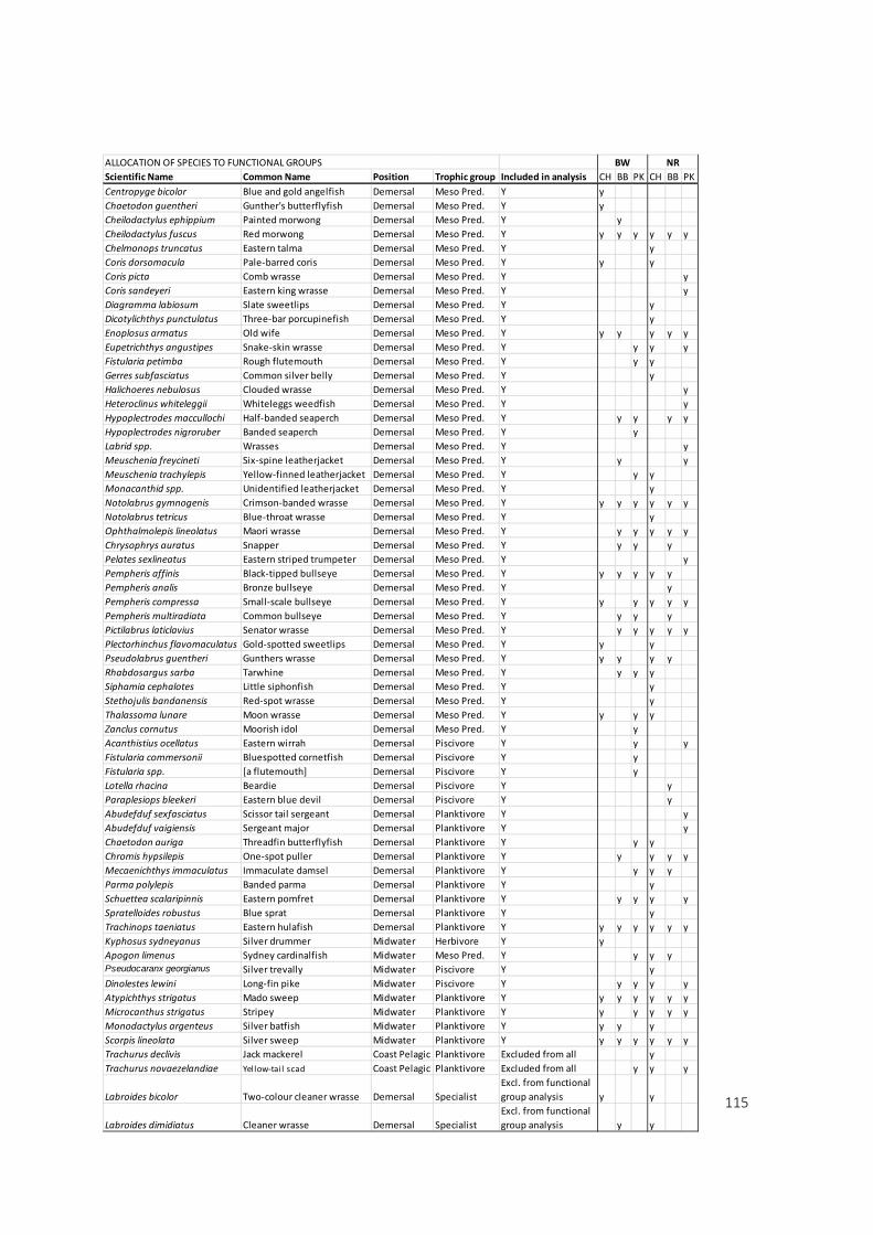
115    

Scientific Name Common Name Position Trophic group Included in analysis CH BB PK CH BB PK

Centropyge bicolor Blue and gold angelfish Demersal Meso Pred. Y y

Chaetodon guentheri Gunther's butterflyfish Demersal Meso Pred. Y y

Cheilodactylus ephippium Painted morwong Demersal Meso Pred. Y y

Cheilodactylus fuscus Red morwong Demersal Meso Pred. Y y y y y y y

Chelmonops truncatus Eastern talma Demersal Meso Pred. Y y

Coris dorsomacula Pale‐barred coris Demersal Meso Pred. Y y y

Coris picta Comb wrasse Demersal Meso Pred. Y y

Coris sandeyeri Eastern king wrasse Demersal Meso Pred. Y y

Diagramma labiosum Slate sweetlips Demersal Meso Pred. Y y

Dicotylichthys punctulatus Three‐bar porcupinefish Demersal Meso Pred. Y y

Enoplosus armatus Old wife Demersal Meso Pred. Y y y y y y

Eupetrichthys angustipes Snake‐skin wrasse Demersal Meso Pred. Y y y y

Fistularia petimba Rough flutemouth Demersal Meso Pred. Y y y

Gerres subfasciatus Common silver belly Demersal Meso Pred. Y y

Halichoeres nebulosus Clouded wrasse Demersal Meso Pred. Y y

Heteroclinus whiteleggii Whiteleggs weedfish Demersal Meso Pred. Y y

Hypoplectrodes maccullochi Half‐banded seaperch Demersal Meso Pred. Y y y y y

Hypoplectrodes nigroruber Banded seaperch Demersal Meso Pred. Y y

Labrid spp. Wrasses Demersal Meso Pred. Y y

Meuschenia freycineti Six‐spine leatherjacket Demersal Meso Pred. Y y y

Meuschenia trachylepis Yellow‐finned leatherjacket Demersal Meso Pred. Y y y

Monacanthid spp. Unidentified leatherjacket Demersal Meso Pred. Y y

Notolabrus gymnogenis Crimson‐banded wrasse Demersal Meso Pred. Y y y y y y y

Notolabrus tetricus Blue‐throat wrasse Demersal Meso Pred. Y y

Ophthalmolepis lineolatus Maori wrasse Demersal Meso Pred. Y y y y y y

Chrysophrys auratus Snapper Demersal Meso Pred. Y y y y

Pelates sexlineatus Eastern striped trumpeter Demersal Meso Pred. Y y

Pempheris affinis Black‐tipped bullseye Demersal Meso Pred. Y y y y y y

Pempheris analis Bronze bullseye Demersal Meso Pred. Y y

Pempheris compressa Small‐scale bullseye Demersal Meso Pred. Y y y y y y

Pempheris multiradiata Common bullseye Demersal Meso Pred. Y y y y

Pictilabrus laticlavius Senator wrasse Demersal Meso Pred. Y y y y y y

Plectorhinchus flavomaculatus Gold‐spotted sweetlips Demersal Meso Pred. Y y y

Pseudolabrus guentheri Gunthers wrasse Demersal Meso Pred. Y y y y y

Rhabdosargus sarba Tarwhine Demersal Meso Pred. Y y y y

Siphamia cephalotes Little siphonfish Demersal Meso Pred. Y y

Stethojulis bandanensis Red‐spot wrasse Demersal Meso Pred. Y y

Thalassoma lunare Moon wrasse Demersal Meso Pred. Y y y y

Zanclus cornutus Moorish idol Demersal Meso Pred. Y y

Acanthistius ocellatus Eastern wirrah Demersal Piscivore Y y y

Fistularia commersonii Bluespotted cornetfish Demersal Piscivore Y y

Fistularia spp. [a flutemouth] Demersal Piscivore Y y

Lotella rhacina Beardie Demersal Piscivore Y y

Paraplesiops bleekeri Eastern blue devil Demersal Piscivore Y y

Abudefduf sexfasciatus Scissor tail sergeant Demersal Planktivore Y y

Abudefduf vaigiensis Sergeant major Demersal Planktivore Y y

Chaetodon auriga Threadfin butterflyfish Demersal Planktivore Y y y

Chromis hypsilepis One‐spot puller Demersal Planktivore Y y y y y

Mecaenichthys immaculatus Immaculate damsel Demersal Planktivore Y y y y

Parma polylepis Banded parma Demersal Planktivore Y y

Schuettea scalaripinnis Eastern pomfret Demersal Planktivore Y y y y y

Spratelloides robustus Blue sprat Demersal Planktivore Y y

Trachinops taeniatus Eastern hulafish Demersal Planktivore Y y y y y y y

Kyphosus sydneyanus Silver drummer Midwater Herbivore Y y

Apogon limenus Sydney cardinalfish Midwater Meso Pred. Y y y yPseudocaranx georgianus Silver trevally Midwater Piscivore Y y

Dinolestes lewini Long‐fin pike Midwater Piscivore Y y y y y

Atypichthys strigatus Mado sweep Midwater Planktivore Y y y y y y y

Microcanthus strigatus Stripey Midwater Planktivore Y y y y y y

Monodactylus argenteus Silver batfish Midwater Planktivore Y y y y

Scorpis lineolata Silver sweep Midwater Planktivore Y y y y y y y

Trachurus declivis Jack mackerel Coast Pelagic Planktivore Excluded from all y

Trachurus novaezelandiae Yellow‐tail  scad Coast Pelagic Planktivore Excluded from all y y y

Labroides bicolor Two‐colour cleaner wrasse Demersal Specialist

Excl. from functional 

group analysis y y

Labroides dimidiatus Cleaner wrasse Demersal Specialist

Excl. from functional 

group analysis   y y

BW NRALLOCATION OF SPECIES TO FUNCTIONAL GROUPS

 

116  

Appendix 2 PERMANOVA results (by species) showing region x contrast interaction. 

Source  df  SS  Pseudo‐F P(perm)

Region (Re)  2  41539  17.8100 0.0001Site (si)  3  22029  1.5102 0.1256   Reef Type  1  12114  1.6705 0.2540Re x Si  6  29173  4.1694 0.0001   Re x Reef Type  2  14503  5.0615 0.0001Residual  60  69970                 Total  71  162710                 

  

Appendix 3 PERMANOVA results for each univariate response at each region. 

Source  df      MS  Pseudo‐F  P(perm)   perms  P(Monte Carlo) 

Total abundance CH  Habitat  1  16.58  0.144  0.752  4  0.739 

Site(Habitat)  2  115.11  2.971 0.072 9947 0.072 Res  20  38.75                                    Total  23                           

BB  Habitat  1  1011.20  14.794  0.249  4  0.058 Site(Habitat)  2  68.36  3.479  0.053  9950  0.051 Res  20  19.65                                    Total  23 

PK  Habitat  1  5361.00  25.812  0.252  4  0.039 Site(Habitat)  2  207.70  3.511  0.054  9956  0.048 Res  20  59.15                              Total  23            

Total Biomass CH  Habitat  1  55.11  0.371  0.753  4  0.626 

Site(Habitat)  2  148.67  1.137 0.336 9954 0.333 Res  20  130.73                                    Total  23         

BB  Habitat  1  4663.00  48.783  0.252  4  0.006  Site(Habitat)  2  95.59  0.608 0.554 9945 0.569  Res  20  157.26                                     Total  23        

 

PK  Habitat  1  7348.90  7.509  0.252  4  0.066 Site(Habitat)  2  978.72  2.952 0.060 9937 0.058 Res  20  331.60                                    Total  23                                            

Richness CH  Habitat  1  1.39  0.188 1.000 3 0.710 

Site(Habitat)  2  7.39  0.730  0.485  8344  0.494 Res  20  10.12                                    Total  23         

BB  Habitat  1  193.39  112.290  0.250  4  0.009 Site(Habitat)  2  1.72  0.244 0.786 7479 0.793 Res  20  7.05                                    Total  23        

PK  Habitat  1  445.01  27.432  0.250  4  0.036 Site(Habitat)  2  16.22  1.195 0.315 9429 0.320 Res  20  13.58                                    Total  23                                            

Functional Richness CH  Habitat  1  1.87  0.091 1.000 4 0.835 

Site(Habitat)  2  20.57  0.168  0.870  9619  0.872 Res  20  122.54                                     Total  23         

BB  Habitat  1  255.80  14.919 0.254 3 0.048 Site(Habitat)  2  17.15  0.156  0.875  8420  0.875 Res  20  109.57                                    

 

117  

 Total  23         

 

PK  Habitat  1  1190.30  7.846  0.250  4  0.087  Site(Habitat)  2  151.70  1.546  0.232  9816  0.231  Res  20  98.10                                     Total  23      

 

β‐Diversity      

CH  Habitat  1  6886.10  1.411  0.252  4  0.219  Site(Habitat)  2  4881.80  2.209  0.000  9857  0.002  Res  20  2210.00                                     Total  23    

 

BB  Habitat  1  8315.90  1.760  0.254  4  0.135  Site(Habitat)  2  4724.90  2.737  0.000  9894  0.001  Res  20  1726.10                                     Total  23               

 

PK  Habitat  1  12721.00  2.562  0.255  4  0.038 Site(Habitat)  2  4965.30  2.463  0.000  9886  0.002 Res  20  2016.10                                    Total  23       

Functional β‐Diversity CH  Habitat  1  3170.50  4.637  0.250  4  0.054 

Site(Habitat)  2  683.69  0.771  0.633  9927  0.616 Res  20  886.29                                    Total  23             

BB  Habitat  1  1149.80  0.897  0.752  4  0.505 Site(Habitat)  2  1282.10  2.190  0.038  9938  0.056 Res  20  585.34                                    Total  23             

PK  Habitat  1  3585.90  1.771  0.255  4  0.242 Site(Habitat)  2  2025.30  2.714  0.012  9941  0.021 Res  20  746.36                                    Total  23        

 

 

Appendix 4 Results of asymmetrical PERMANOVA (by species) at each region comparing reef types (breakwall vs 

natural reef). Monte‐Carlo corrected p‐values are included for interpretation of results with few (<10) unique 

permutations. 

Source  df  SS  MS  Pseudo‐F P(perm) perms P (Monte Carlo) 

Coffs Harbour     Reef Type  1  5076.2  5076.2 1.2876 0.2498 4 0.2969 Site (Reef type)  2  7884.4  3942.2 2.6572 0.0001 9871 0.0011 Res  20  29672  1483.6                           Total  23  42632                             Botany Bay             Reef Type  1  6241.1  6241.1 2.031 0.2589 4 0.1328 Site (Reef Type)  2  6146  3073  3.9666 0.0001 9910 0.0002 Res  20  15494  774.71                           Total  23  27881                                    Port Kembla                   Reef Type  1  13139  13139 3.0941 0.2577 4 0.0449 Site (Reef Type)  2  8492.8  4246.4 3.2195 0.0001 9906 0.001 Res  20  26379  1319                            Total  23  48011              

 

 

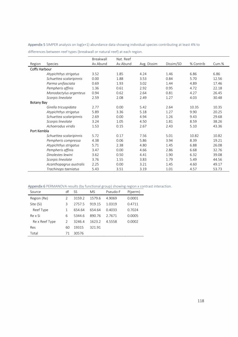
118  

Appendix 5 SIMPER analysis on log(x+1) abundance data showing individual species contributing at least 4% to 

differences between reef types (breakwall or natural reef) at each region. 

  

Breakwall Nat. Reef                        Region  Species  Av.Abund Av.Abund Avg. Dissim Dissim/SD  % Contrib Cum.%

Coffs Harbour       Atypichthys strigatus  3.52 1.85 4.24 1.46  6.86 6.86  Schuettea scalaripinnis  0.00 1.88 3.53 0.84  5.70 12.56  Parma unifasciata  0.69 1.93 3.02 1.44  4.89 17.46  Pempheris affinis  1.36 0.61 2.92 0.95  4.72 22.18  Monodactylus argenteus  0.94 0.62 2.64 0.81  4.27 26.45  Scorpis lineolate  2.59 2.08 2.49 1.27  4.03 30.48Botany Bay       Girella tricuspidata  2.77 0.00 5.42 2.64  10.35 10.35  Atypichthys strigatus  5.89 3.36 5.18 1.27  9.90 20.25  Schuettea scalaripinnis  2.69 0.00 4.94 1.26  9.43 29.68  Scorpis lineolate  3.24 1.05 4.50 1.81  8.59 38.26  Achoerodus viridis  1.53 0.15 2.67 2.43  5.10 43.36Port Kembla       Schuettea scalaripinnis  5.72 0.17 7.56 5.01  10.82 10.82  Pempheris compressa  4.38 0.06 5.86 3.94  8.39 19.21  Atypichthys strigatus  5.71 2.38 4.80 1.45  6.88 26.08  Pempheris affinis  3.47 0.00 4.66 2.86  6.68 32.76  Dinolestes lewini  3.62 0.50 4.41 1.90  6.32 39.08  Scorpis lineolate  3.76 1.55 3.83 1.79  5.49 44.56  Acanthopagrus australis  2.25 0.00 3.21 1.45  4.60 49.17  Trachinops taeniatus  5.43 3.51 3.19 1.01  4.57 53.73

 

 

Appendix 6 PERMANOVA results (by functional group) showing region x contrast interaction. 

Source  df  SS  MS  Pseudo‐F  P(perm) 

Region (Re)  2  3159.2  1579.6  4.9069  0.0001 

Site (Si)  3  2757.5  919.15  1.0319  0.4711 

   Reef Type  1  654.64  654.64  0.4033  0.7024 

Re x Si  6  5344.6  890.76  2.7671  0.0005 

   Re x Reef Type  2  3246.4  1623.2  4.5558  0.0002 

Res  60  19315  321.91                    

Total  71  30576         

 

 

119  

Appendix 7 Results of asymmetrical PERMANOVA (by functional group) at each region comparing reef types 

(breakwall vs natural reef). Monte‐Carlo corrected p‐values are included for interpretation of results with few 

unique permutations. 

Source  df  SS  MS  Pseudo‐F P(perm) perms P(Monte Carlo) 

Coffs Harbour            Reef Type  1  654.6  654.6  0.6226 0.5076 4 0.6192 Site(Reef Type)  2  2102.8  1051.4  2.5701 0.0202 9953 0.0204 Res  68  27818  409.1 Total  71  30576   Botany Bay               Reef Type  1  456.1  456.1  0.7170 0.7505 4 0.5571 Site(Reef Type)  2  1272.2  636.1  2.628 0.0335 9961 0.0439 Res  20  4841  242.05 Total  23  6569.3   Port Kembla               Reef Type  1  1741.1  1741.1  1.3996 0.4978 4 0.3433 Site(Reef Type)  2  2487.9  1244  3.7595 0.0075 9956 0.0177 Res  20  6617.8  330.89 Total  23  10847   

  Appendix 8 SIMPER analysis on Presence/Absence transformed Funtio‐Trophic groups at each region. 

Region  Functio‐Trophic Group BreakwallAv.Abund 

Nat. ReefAv.Abund  Av.Dissim  Dissim/SD  Contrib%  Cum.% 

Coffs Harbour        Planktivore Dem 0.17  0.78 6.60 1.43 21.00  21.00  Infauna Pred. Benthic  0.50  0.17 4.87 0.97 15.49  36.49  Infauna Pred. Dem  0.50  0.39 4.87 0.97 15.49  51.98  Meso Pred. Benthic  0.33  0.28 4.00 0.85 12.73  64.71  Piscivore Midwat 0.00  0.39 3.62 0.79 11.52  76.23  Piscivore Benthic 0.33  0.11 3.49 0.76 11.10  87.33  Herbivore Midwat  0.33  0.00 3.02 0.69 9.61  96.94Botany Bay       Infauna Pred. Dem  0.50  0.28 4.97 0.99 23.43  23.43  Piscivore Midwat 0.50  0.00 4.90 0.98 23.10  46.54  Piscivore Benthic 0.17  0.39 4.16 0.85 19.64  66.18  Infauna Pred. Benthic  0.17  0.06 2.13 0.50 10.07  76.25  Planktivore midwat  1.00  0.83 1.83 0.44 8.63  84.88  Meso Pred. Midwat  0.00  0.17 1.52 0.44 7.18  92.05Port Kembla       Piscivore Midwat 1.00  0.33 6.04 1.38 21.49  21.49  Meso Pred. Midwat  0.67  0.00 5.70 1.38 20.26  41.75  Piscivore Dem  0.50  0.11 4.41 0.98 15.68  57.43  Infauna Pred. Dem  0.50  0.44 4.36 0.99 15.52  72.95  Planktivore midwat  1.00  0.78 2.20 0.53 7.83  80.78  Infauna Pred. Benthic  0.00  0.22 1.80 0.53 6.42  87.20  Planktivore Dem 1.00  0.83 1.58 0.44 5.62  92.82

 

 

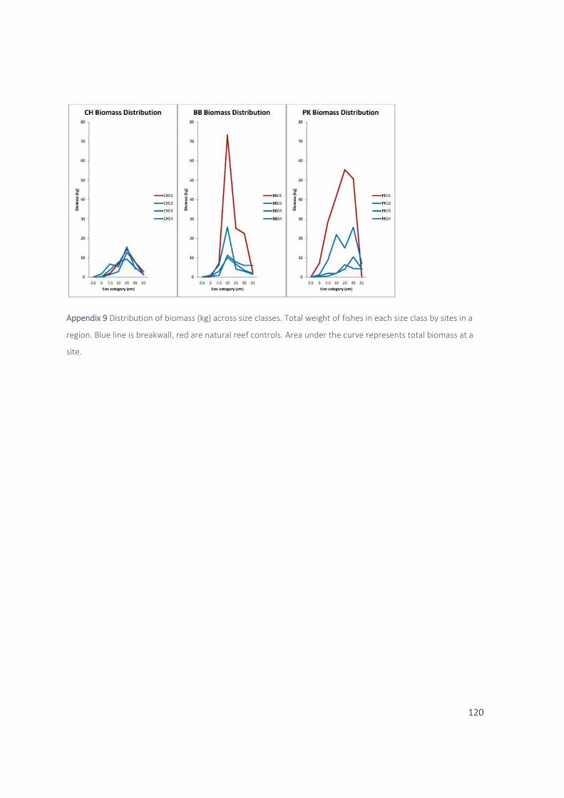
120  

 

Appendix 9 Distribution of biomass (kg) across size classes. Total weight of fishes in each size class by sites in a 

region. Blue line is breakwall, red are natural reef controls. Area under the curve represents total biomass at a 

site. 

 

121  

Chapter 3 Appendices 

Appendix 3.1  “complexity‐metrics” software 

A custom software was developed in conjunction with Dr. Mitchell Bryson of the Australian Centre for Field 

Robotics. See http://www‐personal.acfr.usyd.edu.au/m.bryson/complexitymetrics for full software package. The 

software performs the following steps to calculate metrics of structural complexity: 

1. Model is read in, bounding box calculated, and virtual quadrats placed. 

Dimensions and orientation of the model are set by the 3D reconstruction software. Bounding 

box is a rectangle encompassing the full extent of the model in X, Y and Z directions. 

2. Position, orientation and size of every face in the model is calculated. 

List of vertices and normals are generated and referenced for each metric calculated. 

3. Surface area and area projected to plane are calculated. 

This is calculated based on both the overall native model X‐Y plane (here termed X/Y plane and 

also based on the local (quadrat) plane of best fit. 

4. Metrics are calculated for the whole model and for each quadrat: 

a. Landscape slope (calculated by least squares of points on plane to mesh surface) 

b. Quadrat fitted slope (as above, for the section of model within each quadrat) 

c. Face angle mean and SD (mean degrees from vertical (facing directly up) of all faces) 

d. Face Angle Histogram (proportion total area of faces in 10 degree vertical angle bins. Face 

angle is the degrees from vertical (facing directly up) of each face) 

e. Overhang (the proportion surface area >= 90 degrees face angle) 

f. Height range aka vertical relief (highest point minus lowest point) 

g. Surface rugosity XY (3D area / 2D area as projected to the XY plane) 

h. Surface rugosity PoBF (3D area / 2D area as projected to the plane of best fit) 

5. Surfaces are re‐interpolated at designated resolutions. For each resolution the following metrics are re‐

calculated: 

i. Height range  

ii. Rugosity XY 

iii. Rugosity PoBF 

User inputs: 

The software package allows the user to specify several parameters that affect the analysis of a 3D model. 

1. Virtual quadrat size and spacing. Quadrats are squares of the size specified. Spacing is from quadrat 

centre to centre. This allows quadrats to overlap, or be spaced apart for independence or other 

reasons. 

2. % quadrat occupied threshold. This number determines how much of a quadrat must be occupied 

before excluding that quadrat from analysis. The default is 90% must be occupied (based on planar 

area). 

3. Resolutions. This list of numbers specifies the resolutions at which the model will be re‐interpolated for 

object size analysis. Any numbers can be specified. However, the finest resolution should not be smaller 

than the model resolution, and the coarsest resolution will be limited by quadrat size (cannot fit a 10m 

triangle in a 2m quadrat). For each resolution value, a grid of that spacing is laid over the original model 

from above. The height values in each cell in the grid are averaged to create a new point and the 

 

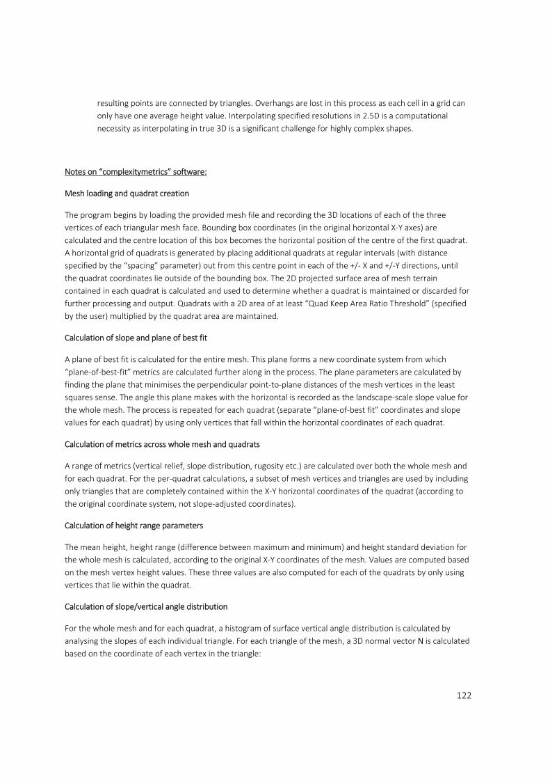
122  

resulting points are connected by triangles. Overhangs are lost in this process as each cell in a grid can 

only have one average height value. Interpolating specified resolutions in 2.5D is a computational 

necessity as interpolating in true 3D is a significant challenge for highly complex shapes. 

 

Notes on “complexitymetrics” software: 

Mesh loading and quadrat creation 

The program begins by loading the provided mesh file and recording the 3D locations of each of the three 

vertices of each triangular mesh face. Bounding box coordinates (in the original horizontal X‐Y axes) are 

calculated and the centre location of this box becomes the horizontal position of the centre of the first quadrat. 

A horizontal grid of quadrats is generated by placing additional quadrats at regular intervals (with distance 

specified by the “spacing” parameter) out from this centre point in each of the +/‐ X and +/‐Y directions, until 

the quadrat coordinates lie outside of the bounding box. The 2D projected surface area of mesh terrain 

contained in each quadrat is calculated and used to determine whether a quadrat is maintained or discarded for 

further processing and output. Quadrats with a 2D area of at least “Quad Keep Area Ratio Threshold” (specified 

by the user) multiplied by the quadrat area are maintained. 

Calculation of slope and plane of best fit 

A plane of best fit is calculated for the entire mesh. This plane forms a new coordinate system from which 

“plane‐of‐best‐fit” metrics are calculated further along in the process. The plane parameters are calculated by 

finding the plane that minimises the perpendicular point‐to‐plane distances of the mesh vertices in the least 

squares sense. The angle this plane makes with the horizontal is recorded as the landscape‐scale slope value for 

the whole mesh. The process is repeated for each quadrat (separate “plane‐of‐best fit” coordinates and slope 

values for each quadrat) by using only vertices that fall within the horizontal coordinates of each quadrat. 

Calculation of metrics across whole mesh and quadrats 

A range of metrics (vertical relief, slope distribution, rugosity etc.) are calculated over both the whole mesh and 

for each quadrat. For the per‐quadrat calculations, a subset of mesh vertices and triangles are used by including 

only triangles that are completely contained within the X‐Y horizontal coordinates of the quadrat (according to 

the original coordinate system, not slope‐adjusted coordinates). 

Calculation of height range parameters 

The mean height, height range (difference between maximum and minimum) and height standard deviation for 

the whole mesh is calculated, according to the original X‐Y coordinates of the mesh. Values are computed based 

on the mesh vertex height values. These three values are also computed for each of the quadrats by only using 

vertices that lie within the quadrat. 

Calculation of slope/vertical angle distribution 

For the whole mesh and for each quadrat, a histogram of surface vertical angle distribution is calculated by 

analysing the slopes of each individual triangle. For each triangle of the mesh, a 3D normal vector N is calculated 

based on the coordinate of each vertex in the triangle: 

 

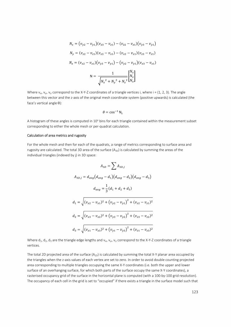
123  

 

 

 

N 1

 

Where vxi, vyi, vzi correspond to the X‐Y‐Z coordinates of a triangle vertices i, where i = (1, 2, 3). The angle 

between this vector and the z‐axis of the original mesh coordinate system (positive upwards) is calculated (the 

face’s vertical angle ): 

cos Nz 

A histogram of these angles is computed in 10o bins for each triangle contained within the measurement subset 

corresponding to either the whole mesh or per‐quadrat calculation. 

Calculation of area metrics and rugosity 

For the whole mesh and then for each of the quadrats, a range of metrics corresponding to surface area and 

rugosity are calculated. The total 3D area of the surface (A3D) is calculated by summing the areas of the 

individual triangles (indexed by j) in 3D space: 

,  

,  

13

 

 

 

 

Where d1, d2, d3 are the triangle edge lengths and vxi, vyi, vzi correspond to the X‐Y‐Z coordinates of a triangle 

vertices.  

The total 2D projected area of the surface (A2D) is calculated by summing the total X‐Y planar area occupied by 

the triangles when the z‐axis values of each vertex are set to zero. In order to avoid double counting projected 

area corresponding to multiple triangles occupying the same X‐Y coordinates (i.e. both the upper and lower 

surface of an overhanging surface, for which both parts of the surface occupy the same X‐Y coordinates), a 

rasterised occupancy grid of the surface in the horizontal plane is computed (with a 100‐by‐100 grid resolution). 

The occupancy of each cell in the grid is set to “occupied” if there exists a triangle in the surface model such that 

 

124  

the cell coordinate lies inside the X‐Y coordinates of the triangle itself. Once each cell has been assessed, the 2D 

area is calculated by summing the number of occupied cells, dividing by the total number of cells and multiplying 

by the total area of the square quadrat. 

Areal rugosity (r) for the surface is then calculated as the ratio between the 2D and 3D surface areas: 

 

Values for 3D area, 2D projected area and rugosity are also computed based on the plane‐of‐best‐fit coordinates 

for the whole mesh or each quadrat. A coordinate transformation is applied to each vertex in the mesh in order 

to place its coordinates in an X‐Y‐Z reference corresponding to the plane‐of‐best‐fit, before calculating the 

metrics as described above. 

Multi‐resolution metric calculation 

In addition to calculating the metrics at the original mesh data, the program provides the ability for the user to 

specify several additional spatial resolutions at which to also calculate metrics. For each specified resolution, the 

program reconstructs a 2.5D approximation of the mesh surface at that resolution by 2D interpolation of the 

surface height value over a regularly spaced grid of X‐Y coordinates, where the distance between points in either 

the X or Y directions is specified by the spatial resolution parameter. For each cell in the defined 2D grid, a vertex 

is created with the corresponding X‐Y coordinates of the cell if at least one part of the original surface passes 

through that point. The z‐coordinate of the vertex is defined by the average of the surface z‐coordinate values 

accounting for all surface triangles within the grid cell. A new set of surface triangles are constructed by joining 

adjacent vertices together in the grid, leaving out sections of the grid for which vertices were not constructed 

(X‐Y locations with no data in the original mesh file). 

Once the reconstructed mesh is created, the whole suit of metrics (vertical relief, slope distribution, rugosity 

etc.) are calculated over this new mesh. Plane‐of‐best fit coordinates for the whole mesh and quadrats are kept 

from those calculated from the original mesh scale when calculating plane‐of‐best‐fit metrics.   

 

Appendix 3.2  Logistic curve fits 

Logistic curves fitted to rugosity loss data for each shape (cone, cube, hemisphere, and rectangle) at each 

resolution (0.125, 1 and 8 cubic m). For each curve Ȓ is calculated as resolution at maximum rugosity loss / 

cubed root volume. 

 

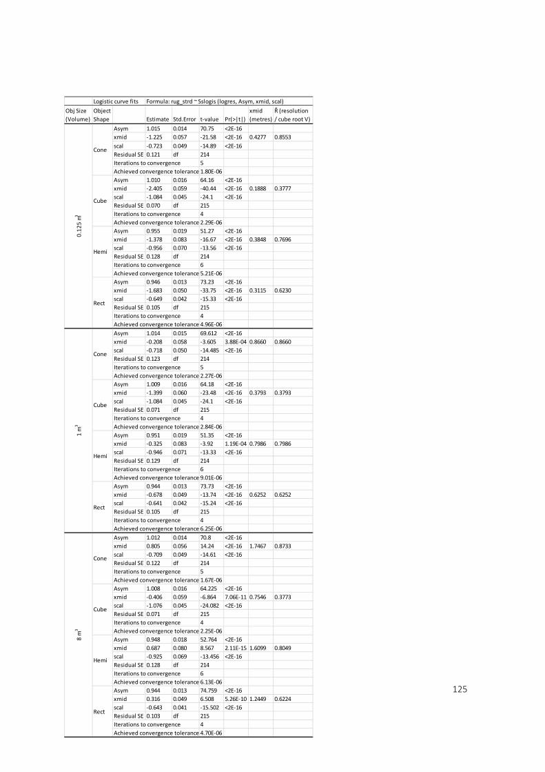
125  

Logistic curve fits Formula: rug_strd ~ Sslogis (logres, Asym, xmid, scal)

Obj Size 

(Volume)

Object 

Shape Estimate Std.Error t‐value Pr(>|t|)

xmid 

(metres)

Ȓ (resolution 

/ cube root V)

Asym 1.015 0.014 70.75 <2E‐16

xmid ‐1.225 0.057 ‐21.58 <2E‐16 0.4277 0.8553

scal ‐0.723 0.049 ‐14.89 <2E‐16

Residual SE 0.121 df 214

Iterations to convergence 5

Achieved convergence tolerance 1.80E‐06

Asym 1.010 0.016 64.16 <2E‐16

xmid ‐2.405 0.059 ‐40.44 <2E‐16 0.1888 0.3777

scal ‐1.084 0.045 ‐24.1 <2E‐16

Residual SE 0.070 df 215

Iterations to convergence 4

Achieved convergence tolerance 2.29E‐06

Asym 0.955 0.019 51.27 <2E‐16

xmid ‐1.378 0.083 ‐16.67 <2E‐16 0.3848 0.7696

scal ‐0.956 0.070 ‐13.56 <2E‐16

Residual SE 0.128 df 214

Iterations to convergence 6

Achieved convergence tolerance 5.21E‐06

Asym 0.946 0.013 73.23 <2E‐16

xmid ‐1.683 0.050 ‐33.75 <2E‐16 0.3115 0.6230

scal ‐0.649 0.042 ‐15.33 <2E‐16

Residual SE 0.105 df 215

Iterations to convergence 4

Achieved convergence tolerance 4.96E‐06

Asym 1.014 0.015 69.612 <2E‐16

xmid ‐0.208 0.058 ‐3.605 3.88E‐04 0.8660 0.8660

scal ‐0.718 0.050 ‐14.485 <2E‐16

Residual SE 0.123 df 214

Iterations to convergence 5

Achieved convergence tolerance 2.27E‐06

Asym 1.009 0.016 64.18 <2E‐16

xmid ‐1.399 0.060 ‐23.48 <2E‐16 0.3793 0.3793

scal ‐1.084 0.045 ‐24.1 <2E‐16

Residual SE 0.071 df 215

Iterations to convergence 4

Achieved convergence tolerance 2.84E‐06

Asym 0.951 0.019 51.35 <2E‐16

xmid ‐0.325 0.083 ‐3.92 1.19E‐04 0.7986 0.7986

scal ‐0.946 0.071 ‐13.33 <2E‐16

Residual SE 0.129 df 214

Iterations to convergence 6

Achieved convergence tolerance 9.01E‐06

Asym 0.944 0.013 73.73 <2E‐16

xmid ‐0.678 0.049 ‐13.74 <2E‐16 0.6252 0.6252

scal ‐0.641 0.042 ‐15.24 <2E‐16

Residual SE 0.105 df 215

Iterations to convergence 4

Achieved convergence tolerance 6.25E‐06

Asym 1.012 0.014 70.8 <2E‐16

xmid 0.805 0.056 14.24 <2E‐16 1.7467 0.8733

scal ‐0.709 0.049 ‐14.61 <2E‐16

Residual SE 0.122 df 214

Iterations to convergence 5

Achieved convergence tolerance 1.67E‐06

Asym 1.008 0.016 64.225 <2E‐16

xmid ‐0.406 0.059 ‐6.864 7.06E‐11 0.7546 0.3773

scal ‐1.076 0.045 ‐24.082 <2E‐16

Residual SE 0.071 df 215

Iterations to convergence 4

Achieved convergence tolerance 2.25E‐06

Asym 0.948 0.018 52.764 <2E‐16

xmid 0.687 0.080 8.567 2.11E‐15 1.6099 0.8049

scal ‐0.925 0.069 ‐13.456 <2E‐16

Residual SE 0.128 df 214

Iterations to convergence 6

Achieved convergence tolerance 6.13E‐06

Asym 0.944 0.013 74.759 <2E‐16

xmid 0.316 0.049 6.508 5.26E‐10 1.2449 0.6224

scal ‐0.643 0.041 ‐15.502 <2E‐16

Residual SE 0.103 df 215

Iterations to convergence 4

Achieved convergence tolerance 4.70E‐06

1 m

38 m

30.125 m

3

Cone

Cube

Hemi

Rect

Cone

Cube

Hemi

Rect

Cone

Cube

Hemi

Rect

 

126  

Appendix 3.3  Ȓ/1D values 

Table 0.1. Resolution at maximum rugosity loss (Ȓ) divided by 1D size of known objects. Variance caused by 

different shapes in bottom row. Variance form calculations done at different sizes in right column. 

 

 

 

 

0.125 m3

1 m3

8 m3

Variance from 

Obj Size (SD)

Cone 0.855 0.866 0.873 0.009

Cube 0.378 0.379 0.377 0.001

Hemisphere 0.770 0.799 0.805 0.019

Rectangle 0.623 0.625 0.622 0.001

Variance from Shape (SD) 0.209 0.217 0.222

Variance from Shape (95% CI) 0.205 0.213 0.217

Overall mean Ȓ/1D 

Mean 95% CI

0.66438

0.21167

Ȓ/1D (resolution @ Max Rug Loss /cube root V) by object size and shape

 

127  

Chapter 4 Appendices 

Appendix 4.1  

Tukey HSD post‐hoc results for structural metrics for each pair‐wise habitat comparison. P‐values adjusted for 

multiple comparisons. 

  

Appendix 4.2 

Dunn’s post‐Hoc test results for structure metrics for each pair‐wise habitat comparison. Bonferroni corrected 

p‐values reported. 

  

Metric Pair‐wise Diff Lower Upper adjusted p

Rugosity CP‐BW ‐0.48 ‐0.72 ‐0.24 < 0.001 *

CS‐BW ‐0.29 ‐0.55 ‐0.02 0.0323 *

RR‐BW ‐0.69 ‐0.90 ‐0.47 < 0.001 *

CS‐CP 0.19 ‐0.05 0.44 0.1603

RR‐CP ‐0.21 ‐0.39 ‐0.03 0.0196 *

RR‐CS ‐0.40 ‐0.63 ‐0.18 < 0.001 *

Vertical relief CP‐BW ‐4.01 ‐5.34 ‐2.68 < 0.001 *

CS‐BW ‐3.39 ‐4.90 ‐1.89 < 0.001 *

RR‐BW ‐3.44 ‐4.65 ‐2.22 < 0.001 *

CS‐CP 0.62 ‐0.75 1.99 0.6312

RR‐CP 0.58 ‐0.46 1.61 0.4623

RR‐CS ‐0.05 ‐1.30 1.21 0.9997

Slope CP‐BW ‐13.79 ‐20.22 ‐7.36 < 0.001 *

CS‐BW ‐13.22 ‐20.50 ‐5.94 < 0.001 *

RR‐BW ‐12.52 ‐18.37 ‐6.67 < 0.001 *

CS‐CP 0.57 ‐6.03 7.17 0.9958

RR‐CP 1.27 ‐3.72 6.26 0.9081

RR‐CS 0.70 ‐5.35 6.75 0.9901

Metric Pair‐wise H p (adj.)

Overhang CP‐BW 3.152 0.0049 *

CS‐BW 2.379 0.0521

RR‐BW 5.343 < 0.001 *

CS‐CP ‐0.725 1.0000

RR‐CP 2.125 0.1009

RR‐CS 2.816 0.0146 *

CP‐BW ‐2.485 0.0389

CS‐BW ‐2.038 0.1246

RR‐BW ‐5.720 < 0.001 *

CS‐CP 0.391 1.0000

RR‐CP ‐3.412 0.0019 *

RR‐CS ‐3.649 < 0.001 *

CP‐BW ‐4.433 < 0.001 *

CS‐BW ‐5.721 < 0.001 *

RR‐BW ‐2.198 0.0839

CS‐CP ‐1.612 0.3209

RR‐CP 3.136 0.0051 *

RR‐CS 4.768 < 0.001 *

Face 

Angle 

Object 

Size Dist.

 

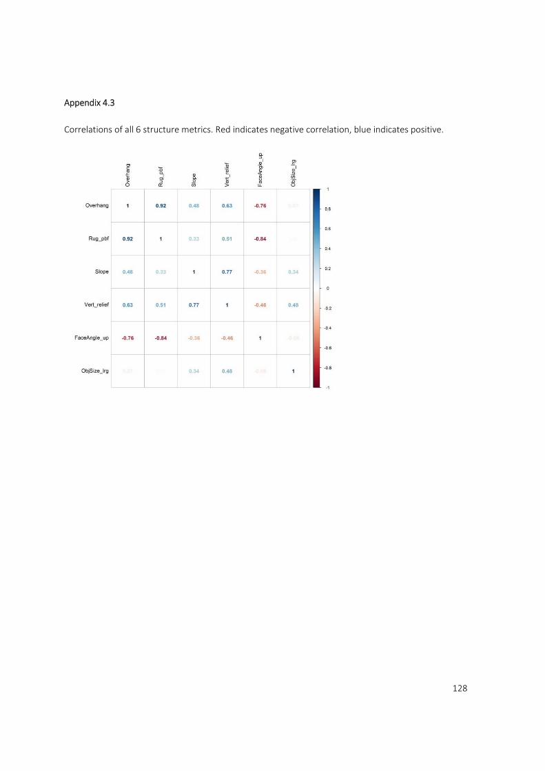
128  

Appendix 4.3 

Correlations of all 6 structure metrics. Red indicates negative correlation, blue indicates positive. 

 

 

129  

 

Appendix 4.4 

Surface rugosity as triangle size increases for 4 habitat types (BW = Breakwall, CP = Coral Patch, CS = Coral Slope, 

RR = Rocky Reef). The first derivative (changes in surface rugosity with decreasing resolution) of each 

relationship approximates the equivalent object size curve in Figure 4.5.  

 

 

 

 

 

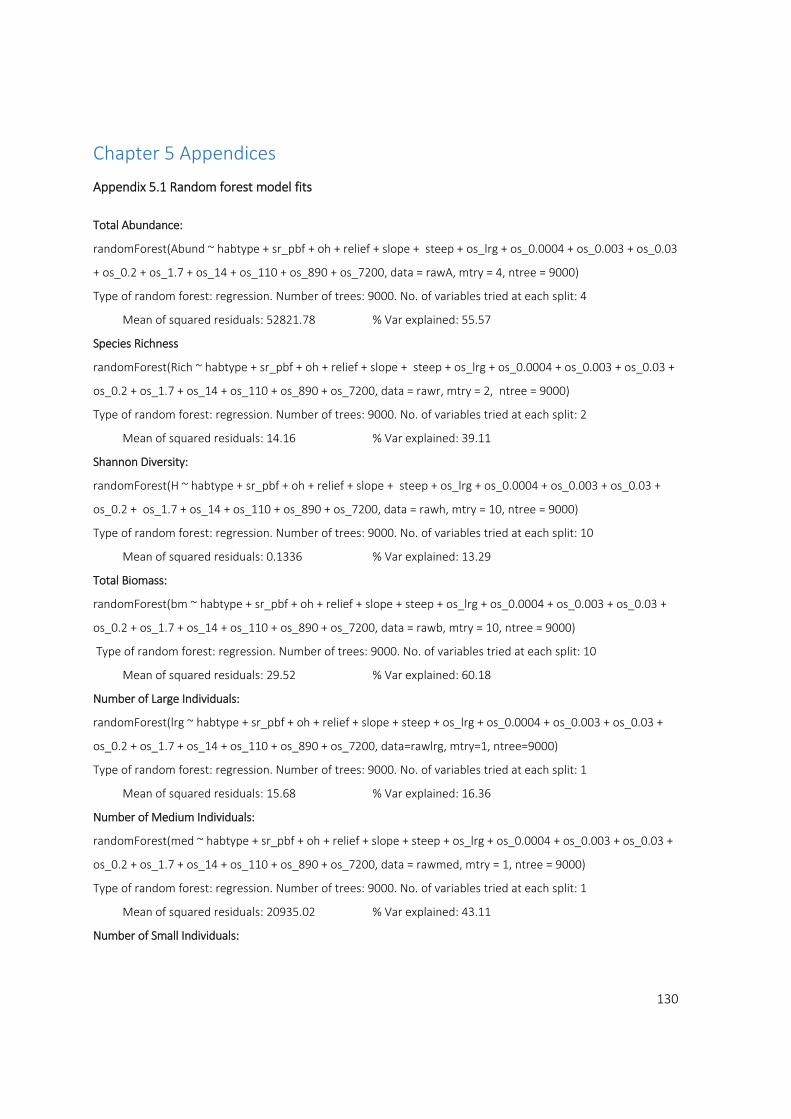
130  

Chapter 5 Appendices 

Appendix 5.1 Random forest model fits 

Total Abundance:  

randomForest(Abund ~ habtype + sr_pbf + oh + relief + slope +  steep + os_lrg + os_0.0004 + os_0.003 + os_0.03 

+ os_0.2 + os_1.7 + os_14 + os_110 + os_890 + os_7200, data = rawA, mtry = 4, ntree = 9000)  

Type of random forest: regression. Number of trees: 9000. No. of variables tried at each split: 4 

          Mean of squared residuals: 52821.78    % Var explained: 55.57 

Species Richness 

randomForest(Rich ~ habtype + sr_pbf + oh + relief + slope +  steep + os_lrg + os_0.0004 + os_0.003 + os_0.03 + 

os_0.2 + os_1.7 + os_14 + os_110 + os_890 + os_7200, data = rawr, mtry = 2,  ntree = 9000)  

Type of random forest: regression. Number of trees: 9000. No. of variables tried at each split: 2 

          Mean of squared residuals: 14.16    % Var explained: 39.11 

Shannon Diversity: 

randomForest(H ~ habtype + sr_pbf + oh + relief + slope +  steep + os_lrg + os_0.0004 + os_0.003 + os_0.03 + 

os_0.2 +  os_1.7 + os_14 + os_110 + os_890 + os_7200, data = rawh, mtry = 10, ntree = 9000)  

Type of random forest: regression. Number of trees: 9000. No. of variables tried at each split: 10 

          Mean of squared residuals: 0.1336    % Var explained: 13.29 

Total Biomass: 

randomForest(bm ~ habtype + sr_pbf + oh + relief + slope + steep + os_lrg + os_0.0004 + os_0.003 + os_0.03 + 

os_0.2 + os_1.7 + os_14 + os_110 + os_890 + os_7200, data = rawb, mtry = 10, ntree = 9000)  

 Type of random forest: regression. Number of trees: 9000. No. of variables tried at each split: 10 

          Mean of squared residuals: 29.52     % Var explained: 60.18 

Number of Large Individuals: 

randomForest(lrg ~ habtype + sr_pbf + oh + relief + slope + steep + os_lrg + os_0.0004 + os_0.003 + os_0.03 + 

os_0.2 + os_1.7 + os_14 + os_110 + os_890 + os_7200, data=rawlrg, mtry=1, ntree=9000)  

Type of random forest: regression. Number of trees: 9000. No. of variables tried at each split: 1 

          Mean of squared residuals: 15.68    % Var explained: 16.36 

Number of Medium Individuals: 

randomForest(med ~ habtype + sr_pbf + oh + relief + slope + steep + os_lrg + os_0.0004 + os_0.003 + os_0.03 + 

os_0.2 + os_1.7 + os_14 + os_110 + os_890 + os_7200, data = rawmed, mtry = 1, ntree = 9000)  

Type of random forest: regression. Number of trees: 9000. No. of variables tried at each split: 1 

          Mean of squared residuals: 20935.02    % Var explained: 43.11 

Number of Small Individuals: 

 

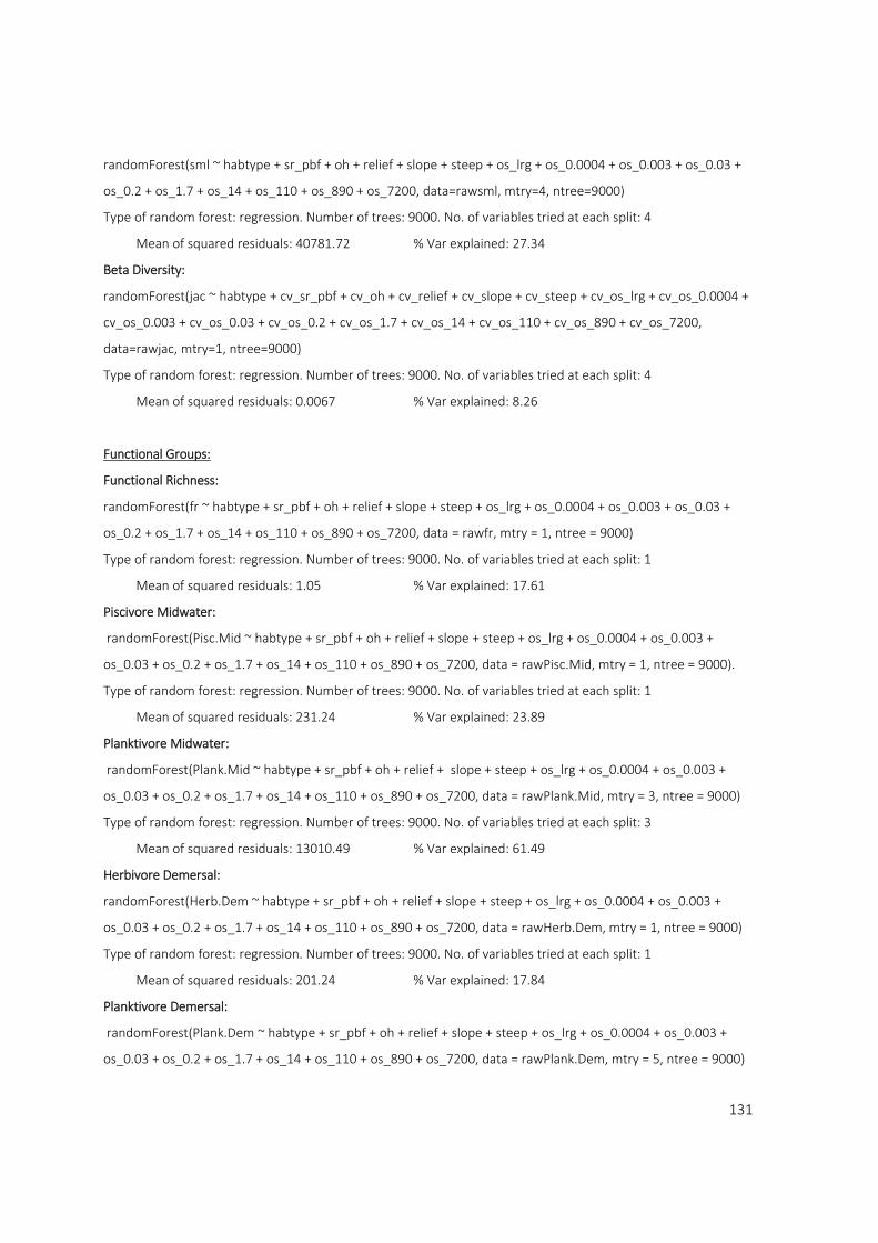
131  

randomForest(sml ~ habtype + sr_pbf + oh + relief + slope + steep + os_lrg + os_0.0004 + os_0.003 + os_0.03 + 

os_0.2 + os_1.7 + os_14 + os_110 + os_890 + os_7200, data=rawsml, mtry=4, ntree=9000)  

Type of random forest: regression. Number of trees: 9000. No. of variables tried at each split: 4 

          Mean of squared residuals: 40781.72    % Var explained: 27.34 

Beta Diversity: 

randomForest(jac ~ habtype + cv_sr_pbf + cv_oh + cv_relief + cv_slope + cv_steep + cv_os_lrg + cv_os_0.0004 + 

cv_os_0.003 + cv_os_0.03 + cv_os_0.2 + cv_os_1.7 + cv_os_14 + cv_os_110 + cv_os_890 + cv_os_7200, 

data=rawjac, mtry=1, ntree=9000)  

Type of random forest: regression. Number of trees: 9000. No. of variables tried at each split: 4 

          Mean of squared residuals: 0.0067    % Var explained: 8.26 

 

Functional Groups: 

Functional Richness: 

randomForest(fr ~ habtype + sr_pbf + oh + relief + slope + steep + os_lrg + os_0.0004 + os_0.003 + os_0.03 + 

os_0.2 + os_1.7 + os_14 + os_110 + os_890 + os_7200, data = rawfr, mtry = 1, ntree = 9000)  

Type of random forest: regression. Number of trees: 9000. No. of variables tried at each split: 1 

          Mean of squared residuals: 1.05    % Var explained: 17.61 

Piscivore Midwater: 

 randomForest(Pisc.Mid ~ habtype + sr_pbf + oh + relief + slope + steep + os_lrg + os_0.0004 + os_0.003 + 

os_0.03 + os_0.2 + os_1.7 + os_14 + os_110 + os_890 + os_7200, data = rawPisc.Mid, mtry = 1, ntree = 9000).  

Type of random forest: regression. Number of trees: 9000. No. of variables tried at each split: 1 

          Mean of squared residuals: 231.24    % Var explained: 23.89 

Planktivore Midwater: 

 randomForest(Plank.Mid ~ habtype + sr_pbf + oh + relief +  slope + steep + os_lrg + os_0.0004 + os_0.003 + 

os_0.03 + os_0.2 + os_1.7 + os_14 + os_110 + os_890 + os_7200, data = rawPlank.Mid, mtry = 3, ntree = 9000)  

Type of random forest: regression. Number of trees: 9000. No. of variables tried at each split: 3 

          Mean of squared residuals: 13010.49    % Var explained: 61.49 

Herbivore Demersal: 

randomForest(Herb.Dem ~ habtype + sr_pbf + oh + relief + slope + steep + os_lrg + os_0.0004 + os_0.003 + 

os_0.03 + os_0.2 + os_1.7 + os_14 + os_110 + os_890 + os_7200, data = rawHerb.Dem, mtry = 1, ntree = 9000)  

Type of random forest: regression. Number of trees: 9000. No. of variables tried at each split: 1 

          Mean of squared residuals: 201.24    % Var explained: 17.84 

Planktivore Demersal: 

 randomForest(Plank.Dem ~ habtype + sr_pbf + oh + relief + slope + steep + os_lrg + os_0.0004 + os_0.003 + 

os_0.03 + os_0.2 + os_1.7 + os_14 + os_110 + os_890 + os_7200, data = rawPlank.Dem, mtry = 5, ntree = 9000)  

 

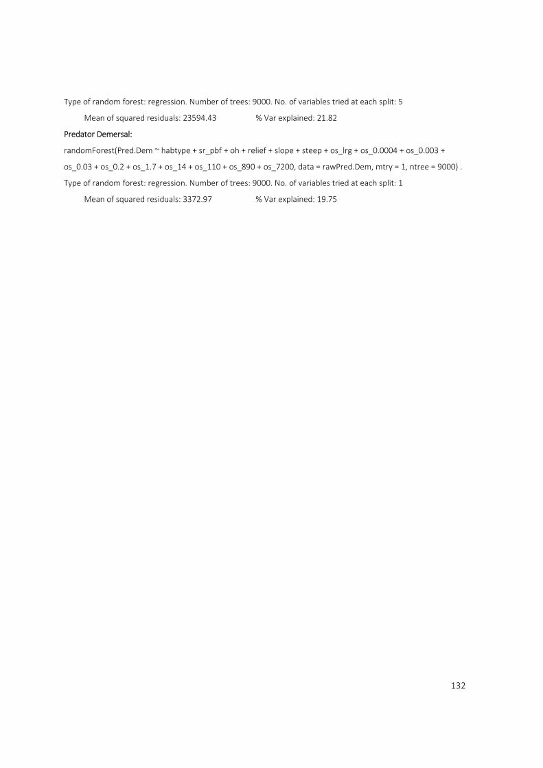
132  

Type of random forest: regression. Number of trees: 9000. No. of variables tried at each split: 5 

          Mean of squared residuals: 23594.43    % Var explained: 21.82 

Predator Demersal: 

randomForest(Pred.Dem ~ habtype + sr_pbf + oh + relief + slope + steep + os_lrg + os_0.0004 + os_0.003 + 

os_0.03 + os_0.2 + os_1.7 + os_14 + os_110 + os_890 + os_7200, data = rawPred.Dem, mtry = 1, ntree = 9000) .  

Type of random forest: regression. Number of trees: 9000. No. of variables tried at each split: 1 

          Mean of squared residuals: 3372.97    % Var explained: 19.75 

 

 

 

133  

Appendix 5.2 Full list of importance plots 

These plots display the relative importance of the predictor variables in driving the responses based 

on the influence each predictor has on all the nodes of each regression tree in random forest analysis.  

 

 

 

 

134  

 

135  

 

 

136  

 

 

137  

 

 

 

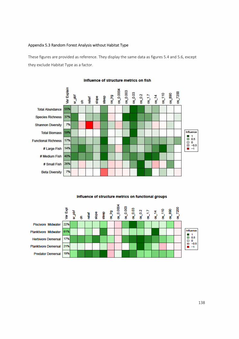
138  

Appendix 5.3 Random Forest Analysis without Habitat Type 

These figures are provided as reference. They display the same data as figures 5.4 and 5.6, except 

they exclude Habitat Type as a factor.