portfolio management

Portfolio ManagementGrenoble Ecole de ManagementMSc Finance2011

Learning Objectives

Mastering the principles of the portfolio management process:

•The minimum variance and the efficient frontier

•Capital Market Line•Capital Asset Pricing Model•Multi-factor models•Asset Pricing Theory

2

Portfolio ManagementThe minimum variance and the efficient frontier

Mean variance analysis

4

Ideas come from an article of 1952 by Harry Markowitz where one can find the mathematic formalization of the common practice of diversification to reduce risk.

Harry Markowitz wrote the basic principles of portfolio construction and propose the first answers to the question: how to determine the optimal weights of each asset in the portfolio ?

This is the mean variance analysis. It is a normative framework.

Mean variance analysis

5

Markowitz’s mean variance analysis is based on the following assumptions:• all investors are risk averse; they prefer less risk

to more for the same level of expected return.• They are able to form expectations on returns for

all assets. • They are able to form expectations on variances

and covariances for all assets. • Investors need only the expected returns,

variances and covariances of returns to determine optimal portfolios. They can ignore skewness, kurtosis and other attributes of a distribution.

• There are no transaction costs or taxes. In practice, to form expectations on returns, variances and covariances investors may use estimation techniques. The estimation of those quantities may be a source of mistakes in decision making when we use mean-variance analysis.

Portfolio of assets: Diversification

6

Variability for selected stocks larger than the variability of the whole portfolio: this the essence of diversification.

Energy Materials 70%-30%Portfolio

St-dev 6.30% 6.65% 5.96%

01/0

1/19

95

01/1

2/19

95

01/1

1/19

96

01/1

0/19

97

01/0

9/19

98

01/0

8/19

99

01/0

7/20

00

01/0

6/20

01

01/0

5/20

02

01/0

4/20

03

01/0

3/20

04

01/0

2/20

05

01/0

1/20

06

01/1

2/20

06

01/1

1/20

07

01/1

0/20

080

50

100

150

200

250

Energy Materials

70%-30% Port

The portfolio possibilities curve – 2 assets

7

20% 21% 22% 23% 24% 25%7.40%

7.60%

7.80%

8.00%

8.20%

8.40%

8.60%

8.80%

9.00%0% Energy - 100% Materials

30% Energy - 70% Materials



A

B

C

Variance

Expected Return


8

• If Energy and Materials were perfectly correlated, the standard deviation of the portfolio would be the weighted average of the two securities standard deviation: portfolios would lie on the dashed line.

• Since correlation is less than 1, the standard deviation of the portfolio of assets is less than the weighted average. The difference between portfolio A and C is the reduction of risk from diversification. A dominates C. It is also true of B that offers larger return for comparable risk.


9

The curvature of the portfolio possibilities curve depends on correlation.Lower correlations increase the curvature and generate higher diversification gains.

Expected Returns

Variance0 50 100 150 200 250

0%

2%

4%

6%

8%

10%

12%

14%

16%

Cor =-0.33 Cor = -1 Cor=1Cor =0.33

Efficient Portfolios – 2 assets

10

20% 21% 22% 23% 24% 25%7.40%

7.60%

7.80%

8.00%

8.20%

8.40%

8.60%

8.80%

9.00% 0% Energy - 100% Materials


Inefficient portfolios

Global minimum variance portfolio 70% Energy - 30% Materials

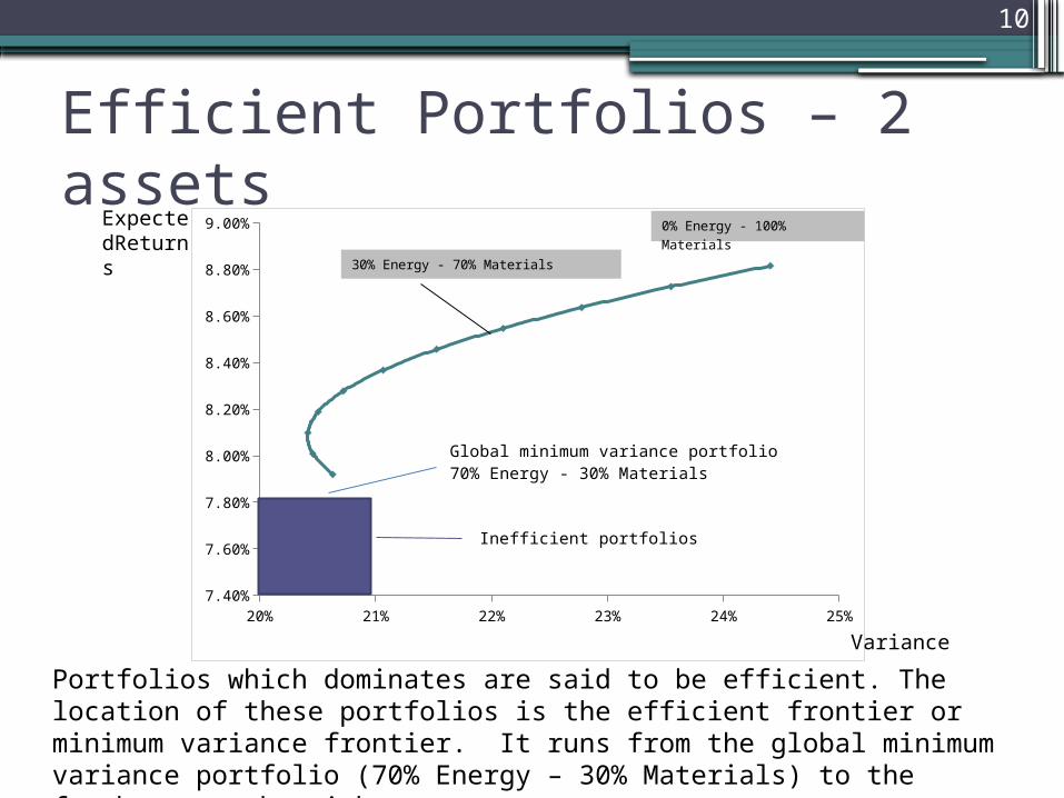
Portfolios which dominates are said to be efficient. The location of these portfolios is the efficient frontier or minimum variance frontier. It runs from the global minimum variance portfolio (70% Energy – 30% Materials) to the farthest on the right.

Variance

ExpectedReturns

Efficient Portfolios – 2 assets

11

The minimum variance portfolio

Efficient Portfolios – n assets

12

Energy

Materials

AA

BBEnergy + Materials + AA + BB portfolio

Standard deviation

Expected return

Often a new asset permits us to move to a superior minimum variance frontier.


13

Efficient portfolios use risk efficiently: every portfolio on the efficient frontier has either a higher rate of return for equal risk or a lower risk for an equal rate of return.Investors making portfolio choices in terms of mean return and variance of return can restrict their selections to portfolios lying on the efficient frontier: this is the selection process


14

Determining the minimum-variance frontier for many assets:• we first determine the minimum and maximum

expected returns possible with the set of assets. These are rmin and rmax

• we must determine the portfolio weights that will create the minimum-variance portfolio for values of expected returns. Between rmin and rmax.

Therefore we must solve the following problem for specified values of r comprise in between rmin and rmax.

This optimization problem says that we solve for the portfolio weights that minimize the variance of return for a given level of expected return r subject to the constraint that the weights sum to 1. The weights define a portfolio and the portfolio is the minimum variance portfolio for its level of expected return.

Min Subject to

Subject to

Min


15

The Lagrangian is:

Min Subject to


16

First order conditions:

Min Subject to


17

Then loading w into the other two conditions yields:

Min Subject to

Solving this system yields:


18

Then reloading in the equation of w we are able to determine the vector w of weights that solve the program for given level of E(Rp):

Min Subject to

This result defines the location of efficient portfolios that solve the optimization program. This location is an hyperbola.

Corner Portfolios

19

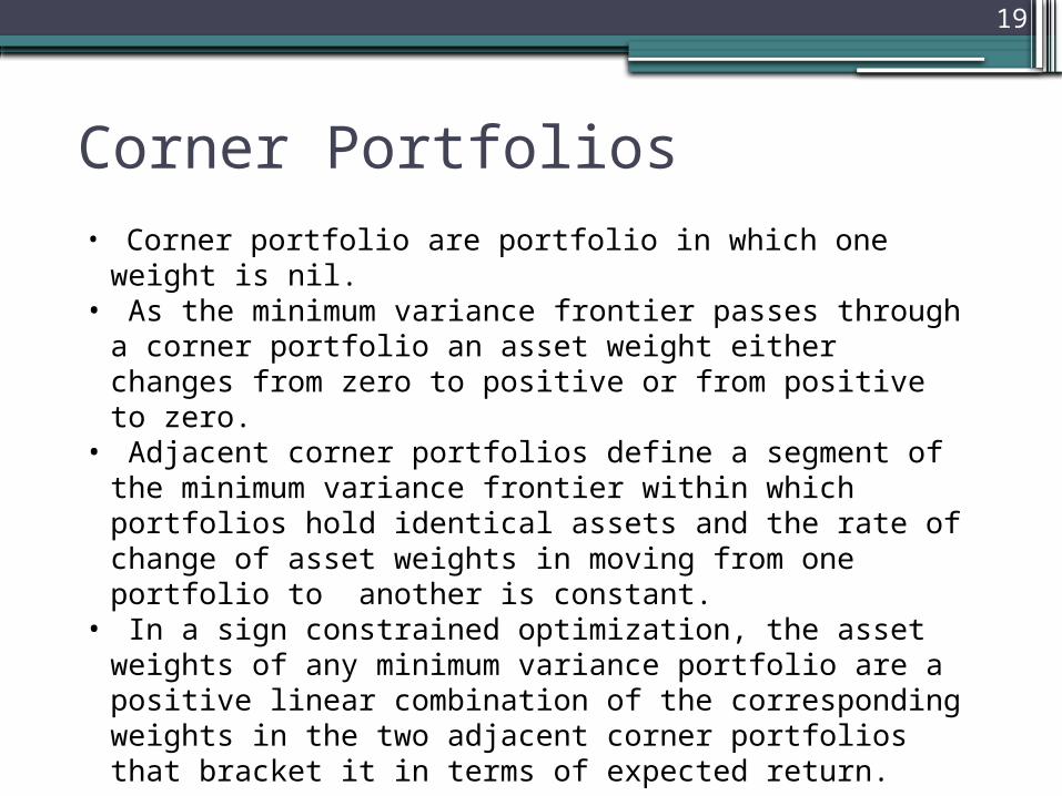
• Corner portfolio are portfolio in which one weight is nil. • As the minimum variance frontier passes through a

corner portfolio an asset weight either changes from zero to positive or from positive to zero.

• Adjacent corner portfolios define a segment of the minimum variance frontier within which portfolios hold identical assets and the rate of change of asset weights in moving from one portfolio to another is constant.

• In a sign constrained optimization, the asset weights of any minimum variance portfolio are a positive linear combination of the corresponding weights in the two adjacent corner portfolios that bracket it in terms of expected return.

Which efficient portfolio ?

20

• If an investor can quantify her/his risk tolerance in terms of variance, the efficient portfolio for that level of variance will represent the optimal mean variance choice.

• However in real life, it is difficult to really quantify risk tolerance then risk scales are often used: 1 no tolerance for risk; 2 low tolerance; 3 medium; 4 high; 5 very high; 6 risk taker.

• In the theoretical framework investors’ preferences are represented by mean of utility functions which associate an ordinal measure of utility to the pair risk/return. Risk adverse investors have convex utility functions. One example of utility function is the quadratic utility function:

Indifference/Utility curves

21

As long as the utility function of the investors is defined, one can derive the indifference curves which set the location of the portfolios providing a constant utility to the investor.

The investor looks at maximizing her/his utility.

Larger utility

Lower utility

22

The tangency point between the efficient frontier and the utility function define the optimal portfolio.

Also optimization under VaR or shortfall constraints in the research section (Moodle) and the document Utility functions and optimization.


The investor looks at maximizing her/his utility under the constraint of the “best” risk/return portfolios: those lying on the efficient frontier.

How to determine optimal weights

23

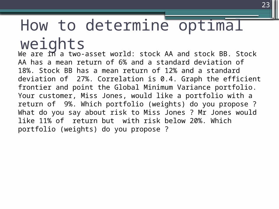
We are in a two-asset world: stock AA and stock BB. Stock AA has a mean return of 6% and a standard deviation of 18%. Stock BB has a mean return of 12% and a standard deviation of 27%. Correlation is 0.4. Graph the efficient frontier and point the Global Minimum Variance portfolio. Your customer, Miss Jones, would like a portfolio with a return of 9%. Which portfolio (weights) do you propose ? What do you say about risk to Miss Jones ? Mr Jones would like 11% of return but with risk below 20%. Which portfolio (weights) do you propose ?

How to determine optimal weights

24

We are in a two-asset world: stock AA and stock BB. Stock AA has a mean return of 6% and a standard deviation of 18%. Stock BB has a mean return of 12% and a standard deviation of 27%. Correlation is -0.3. Graph the efficient frontier and point the Global Minimum Variance portfolio. Your customer, Miss Jones, would like a portfolio with a return of 9%. Which portfolio (weights) do you propose ? What do you say about risk to Miss Jones ? Mr Jones would like 11% of return but with risk below 20%. Which portfolio (weights) do you propose ?

Summary

25

• When correlations are less than 1, they offer diversification opportunities

• Diversified portfolios lie on the possibilities curve.• Portfolios which dominates are said to be efficient. The

location of these portfolios is the efficient frontier or minimum variance frontier.

• If an investor can quantify his risk tolerance in terms of variance, the efficient portfolio for that level of variance will represent the optimal mean variance choice.

Lending and Borrowing

26

We introduce another possibility: we can also lend and borrow money at some risk-free rate rf.

If we invest some money in T-bill (lend money) and place the remainder in common stock portfolio we can obtain any combination of expected return and risk along the straight line joining rf and the S portfolio.

rfInefficient portfolios (combination of rf and T)

efficient portfolios (combination of rf and S)

T

S

Expected returns

Sd dev


27

Since borrowing is negative lending we can extend the range of possibilities to the right of the market portfolio

rfborrowing

lending

S

Expected returns

Sd dev


28

S has an expected return of 15% and a Sd-dev of 25%. T-bill offer a risk-free rate (rf) of 5%. If you invest half your money in T-bill and half in S. What is the expected return of your portfolio ? Its st-dev ?

Then you borrow at rf an amount initial to your original wealth and you invest everything in portfolio S. What is the expected return of your portfolio ? Its st-dev ?

Capital allocation line

29

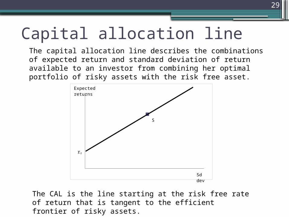
The capital allocation line describes the combinations of expected return and standard deviation of return available to an investor from combining her optimal portfolio of risky assets with the risk free asset.

rf

S

Expected returns

Sd dev

The CAL is the line starting at the risk free rate of return that is tangent to the efficient frontier of risky assets.


30

• If we can invest in a risk-free asset, then the CAL represents the best risk return trade-off achievable.

• The CAL has a y-intercept equal to the risk-free rate.

• The CAL is tangent to the efficient frontier of risky assets.

CAL Equation

31

Suppose an investor facing a risk-free rate of rf has expectations for the S portfolio of E(Rt) and σ(Rt). The return of his portfolio is:

And st-dev is:

Then we can rewrite wt as:

If we substitute wt in the expected return equation:

CAL Equation

32

This equation shows the best possible trade-off between expected risk and return, given this investor’s expectations

rf

S

Expected returns

Sd dev

Capital Market Line

33

• In the mean variance analysis, investors are able to form expectations about return and variance for all assets. They have the same expectations. Thus they all hold the same portfolio. This is the Market portfolio M.

• The proportion of each asset in that portfolio are the same for all investors. Thus the efficient portfolio is a market capitalization weighted basket of securities.

• The sum of all portfolios held by investors constitute the market portfolio, of which every investor holds a proportionate share

• when investors share identical expectations, the CAL for all investors is the same and is known as the Capital Market Line – CML -

Capital Market Line

34

The slope of the CML, is called the market price of risk. It is the amount of return in excess of the risk free rate per unit of risk.

Also we can define this ratio for any portfolio lying on the CAL:

This ratio is known as the Sharpe ratio

Capital Market Line

35

• The market portfolio is the core component of asset pricing as well as the theoretical foundation for index investing. If the market portfolio is efficient allocation, then there is no role for active investing. All investors can satisfy their investment needs by combining the risk-free asset with the market portfolio.

• But if you think you have better information than your rivals you will want the portfolio to include relatively large investments in the stocks you think are undervalued. This is active investment.

36


37

The separation theorem

• First investors form expectations and invest in portfolio M that lies on the efficient frontier. If returns are known M is unique.

• Second investors estimate their risk tolerance and decide to lend or borrow money to reach a certain point of risk on the Capital Market Line.

• Tobin(1958) has called this separation of the investment decision from the financing decision the separation theorem.

38

CAL calculationsThe risk-free rate is 5%, the expected return to an investor’s tangency portfolio is 15% and the St-dev of the tangency portfolio is 25%.1) How much return does this investor demand in order to take on an extra unit

of risk?2) The investors wants a portfolio sd-dev of 10%. Which are the weights of the

risk-free rate and the tangency portfolio in his own portfolio ?3) The investor wants to put 40% of the portfolio in the risk free asset. What is

the return and the sd-dev of this portfolio ?4) What return can expect the investor for a portfolio with sd-dev of 35% ?5) If the investor has EUR10 million to invest, how much she borrow at the risk-

free rate to have a portfolio with an expected return of 19% ?

Summary

39

• The Capital Allocation Line describes the combinations of expected return and standard deviation of return available to an investor from combining her optimal portfolio of risky assets with the risk free asset.

• The CAL is tangent to the efficient frontier of risky assets.

• When investors share identical expectations, the CAL for all investors is the same and is known as the Capital Market Line – CML. The tangency portfolio is the Market portfolio.

• The slope of the CML, is called the market price of risk.• If an investor can quantify his risk tolerance in terms of

variance, the portfolio lying on the CML for that level of variance will represent the optimal mean variance choice.

Portfolio ManagementCapital Asset Pricing ModelMultifactor modelsAPT

Capital Asset Pricing Model

41

The CML states a relationship between risk and returns at the portfolio level when expected returns are known: • more risk calls for more return• the relationship is linear • it enables one to choose an allocation according to ones

risk tolerance in a two-step procedure (investment – financing).

Mean-variance optimization is a tool to estimate the location of the efficient frontier and the M portfolio .

However it needs to be fed with large quantities of data mainly because the number of covariances increases in the square of the number of securities.


42

To simplify this analysis, Sharpe has proposed to consider that expected returns for any asset i depends on:• a common unique factor (which has turned to be the

expected return of the market portfolio)• the sensitivity of the return on asset i to the return on

the market returns βi • the part of returns on asset i that are independent of

market returns α i

This greatly reduce the computational task of providing the inputs to a mean-variance optimization.

The most convenient way to estimate these parameters is to estimate a linear regression using time-series data on the returns to the market and returns to each asset.


43

The number of parameters a portfolio manager needs to estimate to determine the minimum-variance frontier depends on the number of potential stocks in the portfolio.

• In a n-stock portfolio, the manager must estimate n variances and n(n-1)/2 covariances, hence a total of n(n+1)/2 parameters.

• Using the beta representation of the universe, the manager has to estimate n variances, the n covariances of the n stocks to the market portfolio and the variance of the market portfolio. Hence 2n+1 parameters.

• For a portfolio of 100 stocks the number of parameters to be estimated decreases from 50050 to 201.

• The beta representation aggregates all the relationship between assets (covariances) in a single parameter: β


44

The use of the CAPM simplifies the estimation of the variance-covariance matrix. It has further implications: it is a single factor equation describing the expected return on any asset as a linear function of its beta.

rf

M

Expected returns

ββi

ri

Security market line: the relation between risk and returns for any asset

1

i


45

Security market line: the relation between risk and returns

rf

M

Expected re-turns

β

GVT Bonds

Corporate bonds

Equities

Equities

Corporate bonds

GVT bonds

T-bill

Less security-more volatility

Absence of residual value risk

Default risk

Interest rate risk

Inflation risk

1

CAPM: simple message

46

The message is simple: in a competitive market, the expected risk premium varies in direct proportion to the beta:

T-bill have a beta of 0 and a premium of 0

The market portfolio has a beta of 1 and a risk premium of

The expected risk premium on an investment with a beta of 0.5 is therefore half the expected risk premium on the market.

CAPM assumptions

47

The CAPM shares most of the assumptions of the mean variance analysis:

• Investors need only know the expected returns, the variances and the covariances of returns to determine which portfolio are optimal for them.

• Investors have identical views about risky assets’ mean returns, variances and correlation.

• Investors can buy and sell assets in any quantities without affecting price and all assets are marketable.

• Investors can borrow and lend at the risk free rate without limit and they can sell short any assets in any quantity.

• Investors pay no taxes on returns and pay no transaction costs

CAPM Equation

48

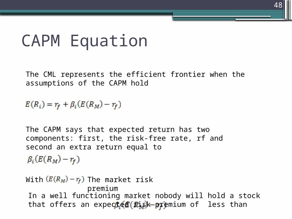
The CML represents the efficient frontier when the assumptions of the CAPM hold

The CAPM says that expected return has two components: first, the risk-free rate, rf and second an extra return equal to

With The market risk premium

In a well functioning market nobody will hold a stock that offers an expected risk premium of less than

CAPM: origin of the equation

49

rf

M

Expected returns

Sd dev

At the tangency point between the possibility curve and the Capital Market Line, the slope of the two are equal

CAPM: origin of the equation

50

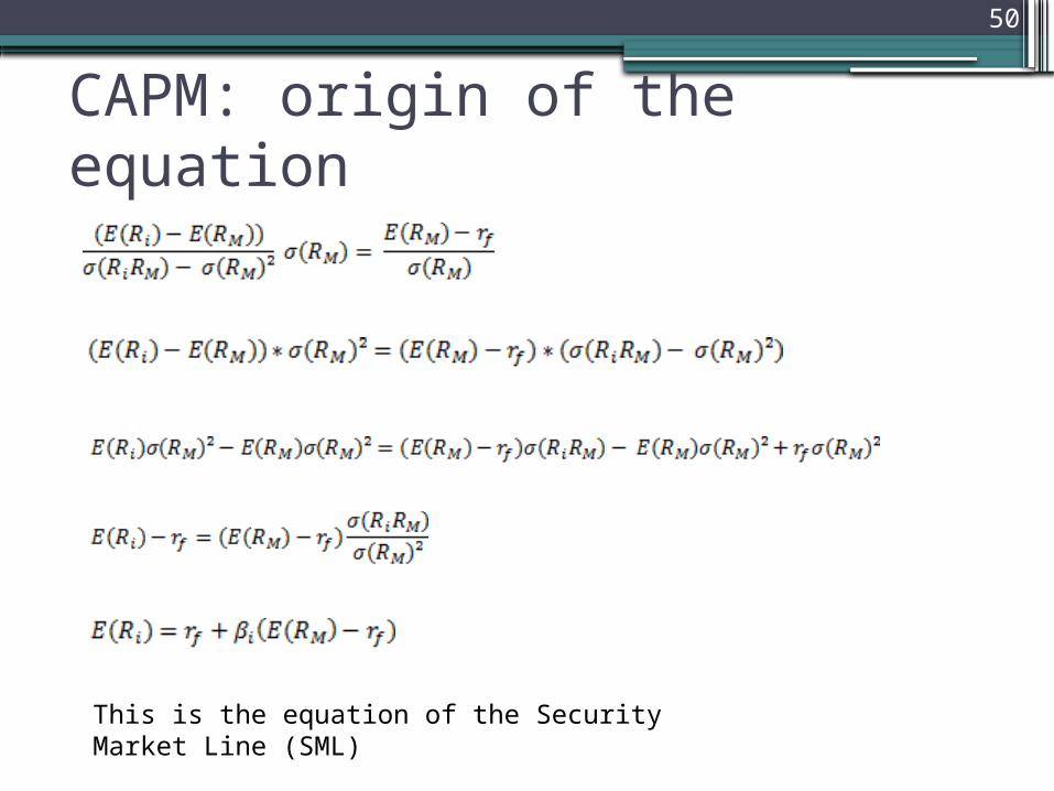
This is the equation of the Security Market Line (SML)

CAPM: estimation

51

The estimation of the equation has the form:

and

Risk can be broken down into which is the residual risk and

which is the systematic risk that cannot be eliminated with

diversification

CAPM: in practice

52

One has to determine an appropriate index to represent the market. In the equity market, domestic equity market index might create a reasonable market model for equities

But using such an index for other asset classes may violate two assumptions of single factor models:• the market return, Rm, is independent of the error term • the error terms are independent across assets.

Then we estimate α and β by using a separate linear regression for each asset. One common practice is to use 60 observations of monthly data.

CAPM: 60-month β

53

-0.2 -0.15 -0.1 -0.05 0 0.05 0.1 0.15-0.15

-0.1

-0.05

0

0.05

0.1

0.15

f(x) = 0.63343542647292 x + 0.004115868810456

Energy sector to MSCI EMU

-0.2 -0.15 -0.1 -0.05 0 0.05 0.1 0.15-0.15

-0.1

-0.05

0

0.05

0.1

0.15

f(x) = 0.6470395118315 x + 0.007223030864

Materials sector to MSCI EMU

-0.2 -0.15 -0.1 -0.05 0 0.05 0.1 0.15-0.3

-0.2

-0.1

0

0.1

0.2

0.3

f(x) = 0.953894175555857 x + 0.00164857052535901

IT sector to MSCI EMU

-0.2 -0.15 -0.1 -0.05 0 0.05 0.1 0.15-0.15

-0.1

-0.05

0

0.05

0.1

0.15

f(x) = 0.639711106302 x + 0.0048591478581

70% energy-30% materials to MSCI EMU

CAPM: 150-month β

54

Energy sector to MSCI EMU Materials sector to MSCI EMU

IT sector to MSCI EMU70% energy-30% materials to MSCI EMU

-0.2 -0.15 -0.1 -0.05 0 0.05 0.1 0.15-0.2

-0.15

-0.1

-0.05

0

0.05

0.1

0.15

0.2

0.25

f(x) = 0.56466089167 x + 0.00645328778

-0.2 -0.15 -0.1 -0.05 0 0.05 0.1 0.15-0.4

-0.3

-0.2

-0.1

0

0.1

0.2

0.3

0.4

f(x) = 1.1582002656 x + 0.00728904663

-0.2 -0.15 -0.1 -0.05 0 0.05 0.1 0.15-0.25

-0.2

-0.15

-0.1

-0.05

0

0.05

0.1

0.15

0.2

f(x) = 0.642630604121 x + 0.005208486747

-0.2 -0.15 -0.1 -0.05 0 0.05 0.1 0.15-0.2

-0.15

-0.1

-0.05

0

0.05

0.1

0.15

0.2

f(x) = 0.586340429387648 x + 0.005847617321545

70%*0.56 + 30% 0.64 = 0.58

CAPM: in practice

55

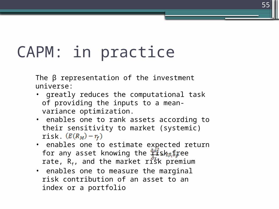
The β representation of the investment universe:• greatly reduces the computational task of

providing the inputs to a mean-variance optimization.

• enables one to rank assets according to their sensitivity to market (systemic) risk.

• enables one to estimate expected return for any asset knowing the risk-free rate, Rf, and the market risk premium

• enables one to measure the marginal risk contribution of an asset to an index or a portfolio

Two empirical critics

56

• The CAPM predicts that beta is the only reason that expected returns differ. However size effects seem to exist: small company stocks performed substantially better than large company stocks. Also stocks with low ratios of market value to book value performed much better than stocks with a high ratio of market to book.

• The security market line has a very small slope. Holding high beta stocks does not offer that much return compared to low beta stocks, especially in recent years.

And three answers

57

• The CAPM is concerned with expected returns only

• In the very long run the relationship is verified but in the short run not

• Before the introduction of CAPM, it was common to assume that one category of investments was suitable for investors with above average willingness and ability to bear risk whereas another category of investments fitted the needs of those with below average risk tolerance. The CAPM concludes however that the market portfolio will efficiently serve all investors’ needs.

Additional theories

58

• C-CAPM defines risk as a stock’s contribution to uncertainty about consumption not wealth. A stock’s expected return should move in line with its consumption beta rather than its market beta

• I-CAPM extends the CAPM above the one period assumption (Merton). Intertemporal CAPM.

CAPM calculations

59

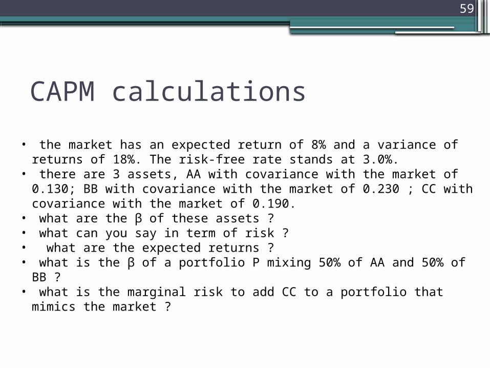
• the market has an expected return of 8% and a variance of returns of 18%. The risk-free rate stands at 3.0%.

• there are 3 assets, AA with covariance with the market of 0.130; BB with covariance with the market of 0.230 ; CC with covariance with the market of 0.190.

• what are the β of these assets ? • what can you say in term of risk ? • what are the expected returns ? • what is the β of a portfolio P mixing 50% of AA and 50% of BB ? • what is the marginal risk to add CC to a portfolio that mimics the

market ?

Multifactor models• The market model assumes that all explainable variation in

asset returns is related to a single factor, the return to the market. Yet asset returns may be related to factors other than market return such as interest rate movements, inflation, or industry specific returns.

• In macro factors models the factors are surprises that significantly explain equity returns.

• In fundamental factor models the factors are attributes like book value to price ratio, market cap, p/e and financial leverage.

• In statistical factors models the factors are the portfolios that best explain historical covariances. In PCA the factors are portfolio that best explain variances.

60

Multifactor models

•Multifactor models explain asset returns better than the market model does.

•Multifactor models provide a more detailed analysis of risk

•They do not rely on the estimation of the location of the market portfolio.

61

Multifactor models

62

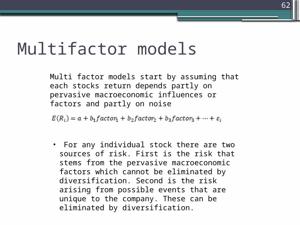
Multi factor models start by assuming that each stocks return depends partly on pervasive macroeconomic influences or factors and partly on noise

• For any individual stock there are two sources of risk. First is the risk that stems from the pervasive macroeconomic factors which cannot be eliminated by diversification. Second is the risk arising from possible events that are unique to the company. These can be eliminated by diversification.

Asset Pricing Theory: APT

63

• the theory does not say what factors are: there could be an oil price factor, an interest-rate factor or the market portfolio or not.

• but it states the condition of market equilibrium:• A diversified portfolio that is constructed to have zero

sensitivity to each factor is essentially risk-free. If this portfolio offers a higher expected return than the risk-free rate, investors can make a risk-free or arbitrage profit by borrowing to buy the portfolio.

• Steven Ross’s Arbitrage pricing theory is based on a multi factor model but it can be applied to single factor models also (the single factor model might be seen as a special case of multi factor models). It starts by assuming that each stocks return depends partly on pervasive macroeconomic influences or factors and partly on noise

APT: Assumptions

64

• A factor model describes asset returns• There are many assets so investors can form well

diversified portfolios that eliminate asset specific risk.

• No arbitrage exist among well diversified portfolios.

• Arbitrage is a risk free operation that earns an expected positive net profit but requires no net investment of money. An arbitrage opportunity is an opportunity to conduct an arbitrage.According to the APT if the above assumptions hold,

the following equation holds:

Where k is the number of factors, λj the risk premium for factor j and βj the sensitivity of the portfolio to factor j.

APT for a single factor representation

65

stocks E(Ri) βi

A 7% 0,5

B 9% 1

C 17% 1,5

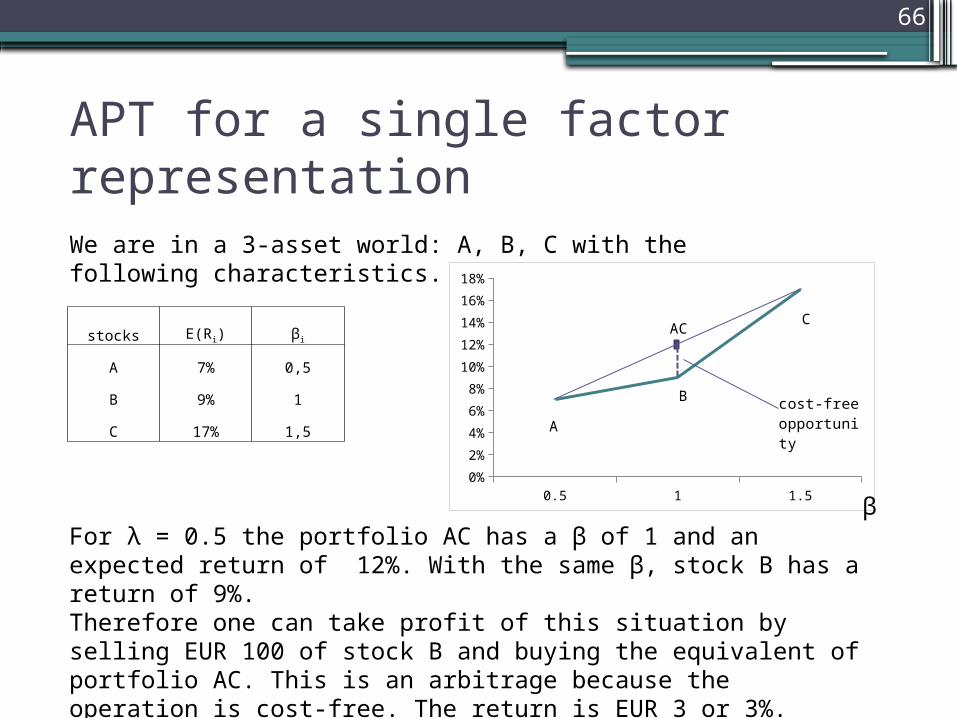
We are in a 3-asset world: A, B, C with the following characteristics.

We can compose a portfolio AC which characteristics will be:

0.5 1 1.50%

2%

4%

6%

8%

10%

12%

14%

16%

18%

A

B

C

β

APT for a single factor representation

66

stocks E(Ri) βi

A 7% 0,5

B 9% 1

C 17% 1,5


For λ = 0.5 the portfolio AC has a β of 1 and an expected return of 12%. With the same β, stock B has a return of 9%. Therefore one can take profit of this situation by selling EUR 100 of stock B and buying the equivalent of portfolio AC. This is an arbitrage because the operation is cost-free. The return is EUR 3 or 3%.

0.5 1 1.50%

2%

4%

6%

8%

10%

12%

14%

16%

18%

A

B

CAC

cost-free op-portunity

β

APT calculations

67


β

stocks E(Ri) βi

A 7% 0,5

B 15% 0,8

C 17% 1,5

Summary

68

• Multifactor models explain asset returns better than the market model does.

• APT states the condition of market equilibrium• Arbitrage is a risk free operation that earns an expected

positive net profit but requires no net investment of money.

• when the market reaches equilibrium, no arbitrage exist among well diversified portfolios.

Capital Markets Expectations

69

• Fundamental law of investing is the uncertainty of the future.

• Capital markets expectations are an essential input to formulating a strategic asset allocation.

• A disciplined approach to expectations setting is key to invest.

• Micro expectations concern individual assets, unique risk.

• Macro expectations concern the market portfolio, systemic risk.

Estimations and previsions

70

rf

M

Expected returns

ββi

ri

Macro factorMicro factors

• Micro factors say where assets stand within the circle• Macro factors say where is the circle in the quadrant• Multi factor models offer a n-dimension analysis of the risk

General Framework

71

1) Specify the final set that are needed, including the time horizon to which they apply.

2) Research the historical record. Most forecasts have some connection to the past.

3) Specify the method and or models that will be used and their information requirements.

4) Determine the best sources for information needs.5) Interpret the current investment environment using the selected

data and methods, applying experience and judgment.6) Provide the set of expectations that are needed, documenting

conclusions.7) Monitor actual outcomes and compare them to expectations,

providing feedback to improve the expectations-setting process.

Macro factors: Macroeconomics

72

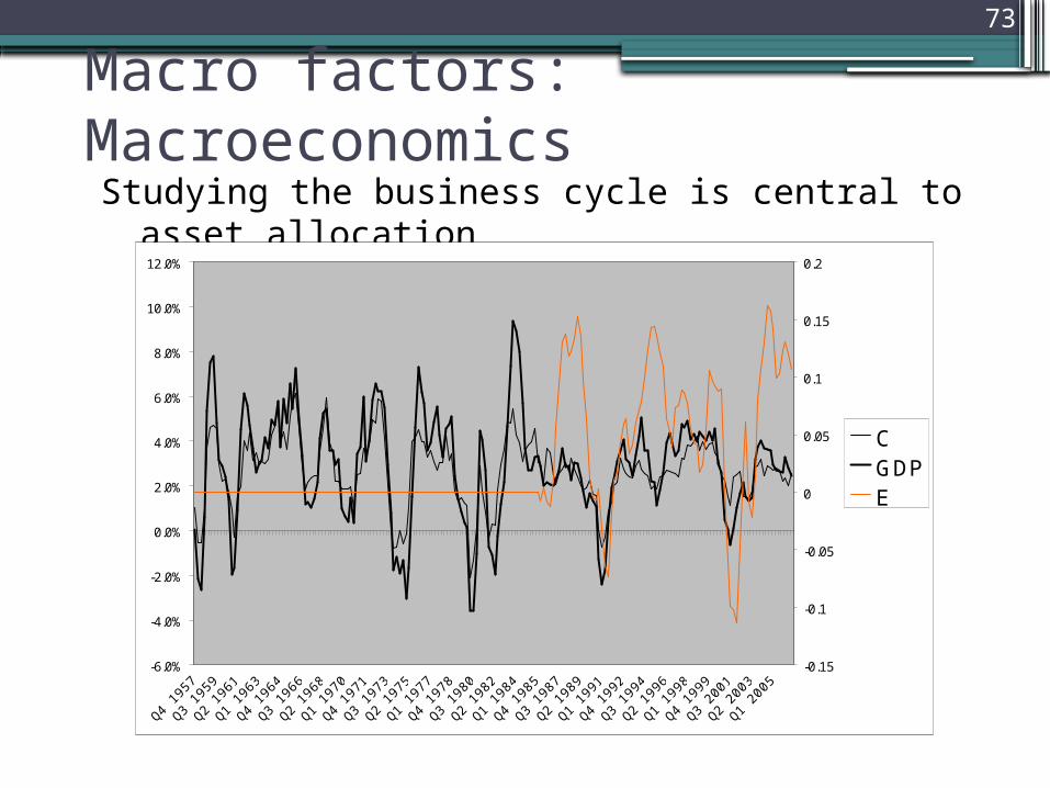
Economic analysis: History has shown that there is a visible relationship between actual realized asset returns, expectations for future asset returns and economic activity.


73

Studying the business cycle is central to asset allocation

-6.0%

-4.0%

-2.0%

0.0%

2.0%

4.0%

6.0%

8.0%

10.0%

12.0%

Q4 19

57

Q3 19

59

Q2 19

61

Q1 19

63

Q4 19

64

Q3 19

66

Q2 19

68

Q1 19

70

Q4 19

71

Q3 19

73

Q2 19

75

Q1 19

77

Q4 19

78

Q3 19

80

Q2 19

82

Q1 19

84

Q4 19

85

Q3 19

87

Q2 19

89

Q1 19

91

Q4 19

92

Q3 19

94

Q2 19

96

Q1 19

98

Q4 19

99

Q3 20

01

Q2 20

03

Q1 20

05

-0.15

-0.1

-0.05

0

0.05

0.1

0.15

0.2

CGDPE

Macro factors models

74

• Chen, Roll and Ross (1986) found that a relatively small set of macro factors was the primary influence on the US stock market.

• These factors are inflation, term structure of interest rate, industrial production and risk aversion measured by the spread between low and high rated corporate bonds.

75

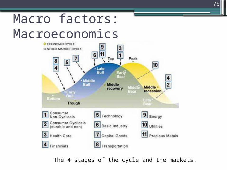
The 4 stages of the cycle and the markets.


76

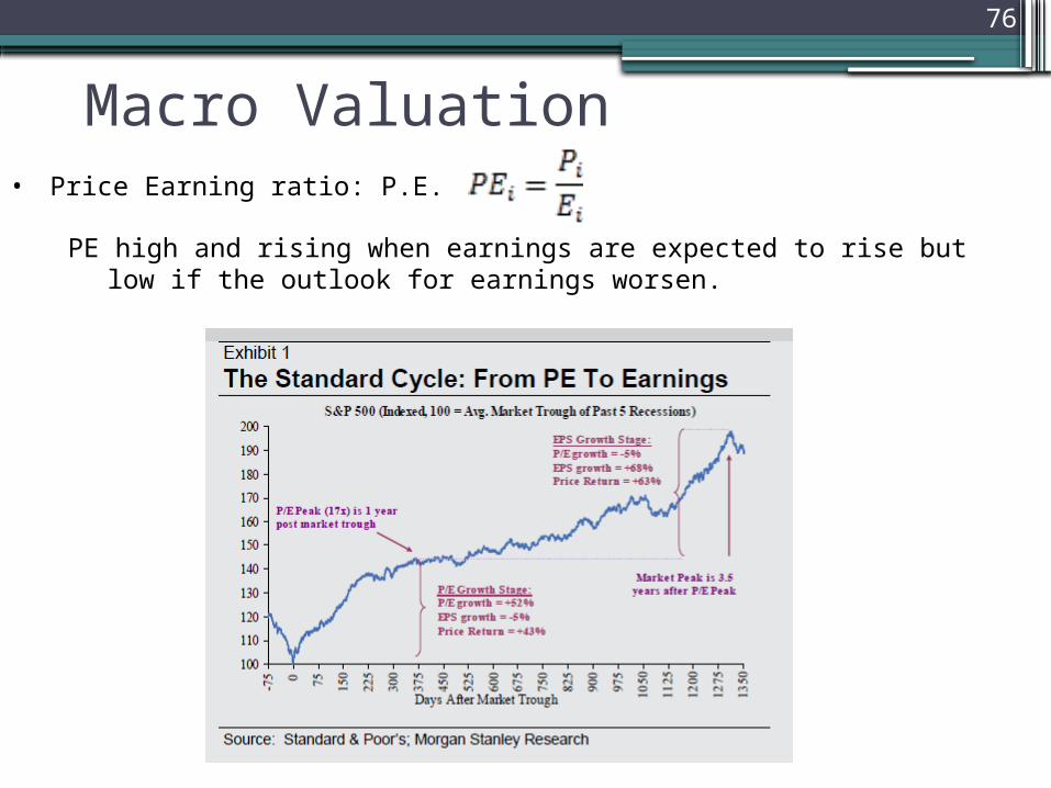
PE high and rising when earnings are expected to rise but low if the outlook for earnings worsen.

Macro Valuation• Price Earning ratio: P.E.

Micro Valuation

77

Discounting cash flows is at the root of any valuation process for individual assets.

• Dividend Discount Model – DDM• Discounted cash flow model• Discounted earning flow model which comes in

different settings (Gordon growth model, Grinold-Kroner model)

Micro Valuation: single factor model

78

• Should we use historical betas from a market model for mean variance

optimization ? Doing so we depend on the crucial assumption that the historical beta is the best predictor of the future beta for that asset.

• Blume (1971) showed that betas tend to be reverting to 1. Therefore adjusted betas predict future betas better than historical betas do.

• One common practice, is to use the following equation:

79

One of the most common ways of classifying a universe of stocks is to divide it into groups based on a fundamental measure. For instance large capitalization stocks versus small capitalization stocks. These groups might be based on:

• factors related to the company’s internal performance. Examples are factors relating to earnings growth, earnings variability, earnings momentum, and financial leverage.

• Factors related to the share price and the valuation of the company. Examples include price multiples such as earnings yield, dividend yield, and book-to-market.

Micro Valuation: multi factor model

80

Stocks with low price/book ratios are categorized as value stocks while stocks with a high price/book are considered growth stocks. Value and growth stocks go through cycles of overperformance and underperformance.

Fama et French (1992) is the most famous multi-factor model based on companies’ fundamentals: it considers a size affect and a book to market effect. http://mba.tuck.dartmouth.edu/pages/faculty/ken.french/

Micro Valuation: value vs growthO

ct-9

6F

eb

-97

Jun

-97

Oct

-97

Fe

b-9

8Ju

n-9

8O

ct-9

8F

eb

-99

Jun

-99

Oct

-99

Fe

b-0

0Ju

n-0

0O

ct-0

0F

eb

-01

Jun

-01

Oct

-01

Fe

b-0

2Ju

n-0

2O

ct-0

2F

eb

-03

Jun

-03

Oct

-03

Fe

b-0

4Ju

n-0

4O

ct-0

4F

eb

-05

Jun

-05

Oct

-05

Fe

b-0

6Ju

n-0

6O

ct-0

6F

eb

-07

Jun

-07

Oct

-07

Fe

b-0

8Ju

n-0

8O

ct-0

8F

eb

-09

Jun

-09

40

50

60

70

80

90

100

110

120

130

140

Value vs growth in the eurozone

Sources of mistakes

81

• Limitations of economic data.• Transcription errors• Survivorship bias• Changes in technological, political legal and regulatory

environments as well as disruption such as wars and other calamities. Such shift in regime give rise to the statistical problem of nonstationnarity.

• Data mining: it is almost inevitable that the analyst will find some statistically significant relationship by mining the data.

• Psychological traps: Anchoring trap (initial impression anchors subsequent thoughts), Status quo, Overconfidence trap

Back to the IPS• We know how to measure risk and return• We are able to determine the beta representation of the

universe.• We know how to classify assets according to their

expected (estimated) risk-return profile• We know how to add-remove one unity of risk because

Beta is a measure of marginal risk.• Thanks to the existence of the risk-free rate, we know

how to reach any risk-return ratio lying on the SML.• We are able to set a portfolio as to respect the investor’s

objectives as mentioned in the IPS• This is no longer ex-post, historical analysis. It is now

sufficient to determine an asset allocation.

82

Summary

• Fundamental law of investing is the uncertainty of the future.

• Studying the business cycle is central to asset allocation

• Discounting cash flows is at the root of any valuation process for individual assets.

• Sources of uncertainty and mistakes are numerous.

83

portfolio management

Documents