portfolio optimization with fuzzy constraints
TRANSCRIPT

Portfolio Optimization with Fuzzy Constraints
Thesis
By: Katalin Santa
Supervisors:
Viktoria Villanyi
Eotvos Lorand University
Robert Fuller
Obuda University
Eotvos Lorand University
2012
Contents
1 Introduction 1
2 Fuzzy sets 3
2.1 Fuzzy sets and logic . . . . . . . . . . . . . . . . . . . . . . . . . . . . 3
2.2 Fuzzy numbers . . . . . . . . . . . . . . . . . . . . . . . . . . . . . . 4
3 Measuring fuzzy numbers 10
3.1 Possibility measure . . . . . . . . . . . . . . . . . . . . . . . . . . . . 11
3.2 Credibility measure . . . . . . . . . . . . . . . . . . . . . . . . . . . . 13
3.2.1 Credibility distribution and density function . . . . . . . . . . 16
3.2.2 Credibility expected value . . . . . . . . . . . . . . . . . . . . 18
4 Portfolio optimization 22
4.1 Markowitz model . . . . . . . . . . . . . . . . . . . . . . . . . . . . . 22
4.2 Markowitz mean-variance model with fuzzy returns . . . . . . . . . . 24
4.2.1 Involving fuzzyness into the model . . . . . . . . . . . . . . . 25
4.2.2 Possibilistic mean-variance with one risk-free asset . . . . . . . 26
4.2.3 Credibilistic mean-variance with one risk-free asset . . . . . . 27
5 Mean-variance model with transaction costs 29
5.1 Hybrid intelligent algorithm . . . . . . . . . . . . . . . . . . . . . . . 30
5.1.1 Fuzzy simulation . . . . . . . . . . . . . . . . . . . . . . . . . 30
5.1.2 Genetic algorithm . . . . . . . . . . . . . . . . . . . . . . . . . 31
Bibliography 35
II
List of Figures
2.1 Triangular fuzzy number with center a . . . . . . . . . . . . . . . . . 5
2.2 Trapezoidal fuzzy number . . . . . . . . . . . . . . . . . . . . . . . . 6
2.3 Membership function of λ ∗ ξ . . . . . . . . . . . . . . . . . . . . . . 7
2.4 Membership function of ξ . . . . . . . . . . . . . . . . . . . . . . . . 8
2.5 Membership function of η . . . . . . . . . . . . . . . . . . . . . . . . 8
2.6 Membership function of ξ ∗ η . . . . . . . . . . . . . . . . . . . . . . . 8
3.1 Pos[A ≤ B] = 1 . . . . . . . . . . . . . . . . . . . . . . . . . . . . . . 11
3.2 Pos[A ≤ B] < 1 . . . . . . . . . . . . . . . . . . . . . . . . . . . . . . 11
3.3 Credibility distribution of a triangular fuzzy variable . . . . . . . . . 16
III

Chapter 1
Introduction
Recently the importance of investment theory is increasing. Not only companies
but also individual investors invest in stock, currency, land and property. It would
be easy to decide where to invest money if we knew future returns a priori, however
uncertainty from i.e. social conditions and behavior have a great influence on the
future returns. The random ambiguous factors, the risk aversion of investors, the
lack of information all take part of this. The problem is to reduce risk while making
profit under such uncertain situations.
We call this problem a portfolio selection problem, which is concerned with se-
lecting a combination of securities to best meet the investor’s desire. The most
influential theory for portfolio selection was proposed by Harry Markowitz. He con-
sidered returns of individual securities as random variables. The key principle of his
mean-variance model was to use the expected return of a portfolio as the investment
return, and the variance as the investment risk.
Since the introduction of Markowitz’s mean-variance model, many efforts have
been made to improve it, and of course made great achievements in portfolio selec-
tion theory. But the common assumption in them are that investors have enough
historical data of securities and that the situation of asset markets in future can be
correctly reflected by asset data in the past. They ignore, for example, the appear-
ance of new stocks, or the above mentioned uncertain situations.
To deal with uncertainty, the focus of portfolio selection began to move towards
fuzzy variables as returns instead of random variables. Fuzzy logic, first proposed by
Lotfi Zadeh, allows expressing uncertain knowledge with subjective concepts, and
uses a higher level of abstraction originating from our knowledge and experience.
Fuzzy logic has been applied in many fields including control theory and artificial
intelligence, and since behavior and human thinking take a great part in portfolio
selection, it seems natural to frame fuzzy logic into portfolio selection problems.
1

In fuzzy portfolio selection there are alternative ways to measure a fuzzy event.
Although possibility, necessity and credibility measures are all popular ways to deal
with uncertainty, this thesis will only consider possibility and credibility as the two
most applied.
Portfolio selection has many different approaches, taking the mean-variance model;
mean-VaR; utility; considering liquidity; with transaction cost; single period model
or rebalancing an existing portfolio, just to mention a few. Taking transaction costs
into consideration is a very important part of finding an effective portfolio. We will
discuss the original problem of mean-variance, and the one with transaction cost,
both with fuzzy returns.
2

Chapter 2
Fuzzy sets
In this chapter we introduce some definitions and examples about fuzzy sets and
numbers. In the second subsection we show a variety of measures for fuzzy sets to
find the one we will use afterwards.
Fuzzy sets were introduced by Lotfi A. Zadeh (1965) as an extension of the
classical set. In classical set theory an element either belongs or does not belong
to the set. So a classical set can be represented by its characteristic function χA
as a mapping from the elements of X to the set of {0, 1}. The value zero repre-
sent the non-membership and the value one represent the membership. What Zadeh
introduced is the following: many sets have more than an either-or criterion for mem-
berships. Take for example the set of tall people. It can be easily decided whether
a 70 cm tall or a 230 cm tall person should be a member of this set. If we’re faced
with a 170 cm tall person then the same question can lead to different answers. (Our
answer will be subjective in this case.)
Zadeh proposed a grade of membership, such that the transition from non-membership
to membership is gradual rather than abrupt. The grade of membership for all its
elements describes a fuzzy set. An item’s grade of membership is normally a real
number between 0 and 1, denoted by µ .
As we use an ordered pair (x, χA(x)) to represent a classical set, we can use tuples
to represent fuzzy sets too. The first element is from X, and the second element
shows the grade of membership of element x in fuzzy set A for x ∈ X.
2.1 Fuzzy sets and logic
Definition 1 [23] Let X be a nonempty set. A fuzzy set A in X is characterized by
its membership function
µA : X → [0, 1]
3
and µA(x) is interpreted as the degree of membership of element in a fuzzy set A for
each x ∈ X.
It should be noted that the terms membership function and fuzzy subset are used
interchangeably and A(x) is often used instead of µA(x).
Example 1 A fuzzy set of real numbers ”close to 5” can be defined as
A(x) = exp(−β(t− 5)2)
where β is a positive real number.
The following definitions are used widely for example in [6], [3], [12], [17] or [7].
Definition 2 An α-level set (or α-cut) of a fuzzy set A of X is a non-fuzzy set
denoted by [A]α and defined by
[A]α = {t ∈ X | A(t) ≥ α}
Definition 3 A fuzzy set is called convex if [A]α is a convex subset for all α ∈ [0, 1].
Definition 4 The support of a fuzzy set A is the set of elements with non-zero
degree of membership.
supp(A) = {x | A(x) > 0}
Definition 5 The core of a fuzzy set A is the set of elements with 1 as degree of
membership.
core(A) = {x | A(x) = 1}
Definition 6 The intersection of fuzzy sets A,B is
min{A(x), B(x)} = A(x) ∧B(x), x ∈ R.
Definition 7 The union of fuzzy sets A,B is
max{A(x), B(x)} = A(x) ∨B(x), x ∈ R.
2.2 Fuzzy numbers
Definition 8 A fuzzy number A is a fuzzy set of the real line with a normal, convex
and upper semi-continuous membership function of bounded support. The family of
fuzzy numbers will be denoted by F
4

Figure 2.1: Triangular fuzzy number with center a
Definition 9 A fuzzy set A is called a triangular fuzzy number with peak (or center)
a, left width α > 0 and right width β > 0 if its membership function has the following
form
A(t) =
1− a−t
αifa− α 5 t 5 a
1− t−aβ
ifa 5 t 5 a+ β
0 otherwise
And we use the notation A = (a, α, β). The support of a triangular fuzzy number A
is (a− α, a + β). A triangular fuzzy number with center a can be considered as: ”x
is approximately equal to a”.
If α = β then we call the triangular fuzzy number symmetrical, and refer to it as
(a, α). Let A = (a, α) and B = (b, β) be two symmetrical triangular fuzzy numbers.
Then
A+B = (a+ b, α + β), λA = (λa, |λ|α)
Definition 10 A fuzzy set A is called a trapezoidal fuzzy number, of it can be de-
termined by four number a < b < c < d; and its membership function µ(x) is as
follows
µ(x) =
1− x−ab−a
ifa ≤ x ≤ b
1 ifb ≤ x ≤ c
1− x−dc−d
ifc ≤ x ≤ d
0 otherwise
and we use the notation A = (a, b, c, d). The support of a trapezoidal fuzzy number
is (a, d). A trapezoidal fuzzy number can be considered as: ”x is approximately in
the interval of [b, c]”.
5

Figure 2.2: Trapezoidal fuzzy number
Definition 11 Any fuzzy number A ∈ F can be described as
A(t) =
L(a−tα
)ift ∈ [a− α, a]
1 ift ∈ [a, b]
R(
t−bβ
)ift ∈ [b, b+ β]
0 otherwise
where [a, b] is the peak or core of A,
L : [0, 1] → [0, 1], R : [0, 1] → [0, 1]
are continuous and non-increasing shape functions with L(0) = R(0) = 1 and L(1) =
R(1) = 0. We call this fuzzy interval of LR-type and refer to it as
A = (a, b, α, β)LR
The support of A is (a− α, b+ β).
In order to introduce fuzzy arithmetic first we have to mention an important
concept from fuzzy set theory called extension principle.
Definition 12 (Zadeh’s extension principle) Let ξ1, ξ2, . . . , ξn are independent fuzzy
variables with membership functions µ1, µ2, . . . , µn, and f : Rn → R. Then the mem-
bership function µ of ξ = f(ξ1, ξ2, . . . , ξn) is derived from the membership functions
µ1, µ2, . . . , µn by
µ(x) = supx=f(x1,x2,...,xn)
min1≤i≤n
µi(xi)
for any x ∈ R. Here we set µ(x) = 0 if there are no x1, x2, . . . , xn such that x =
f(x1, x2, . . . , xn).
6
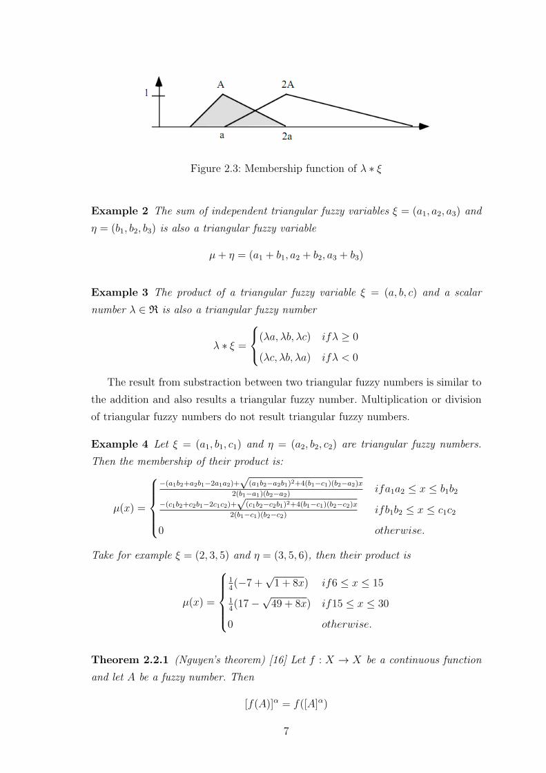
Figure 2.3: Membership function of λ ∗ ξ
Example 2 The sum of independent triangular fuzzy variables ξ = (a1, a2, a3) and
η = (b1, b2, b3) is also a triangular fuzzy variable
µ+ η = (a1 + b1, a2 + b2, a3 + b3)
Example 3 The product of a triangular fuzzy variable ξ = (a, b, c) and a scalar
number λ ∈ R is also a triangular fuzzy number
λ ∗ ξ =
(λa, λb, λc) ifλ ≥ 0
(λc, λb, λa) ifλ < 0
The result from substraction between two triangular fuzzy numbers is similar to
the addition and also results a triangular fuzzy number. Multiplication or division
of triangular fuzzy numbers do not result triangular fuzzy numbers.
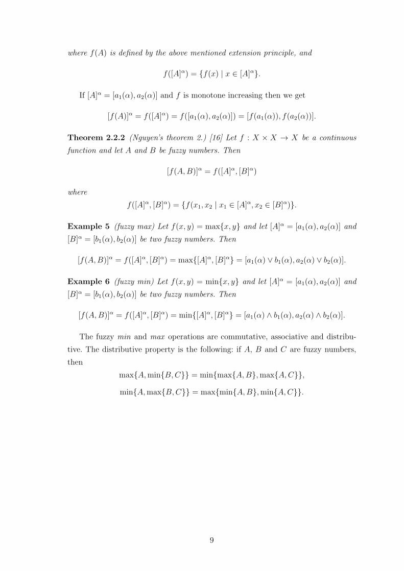
Example 4 Let ξ = (a1, b1, c1) and η = (a2, b2, c2) are triangular fuzzy numbers.
Then the membership of their product is:
µ(x) =
−(a1b2+a2b1−2a1a2)+
√(a1b2−a2b1)2+4(b1−c1)(b2−a2)x
2(b1−a1)(b2−a2)ifa1a2 ≤ x ≤ b1b2
−(c1b2+c2b1−2c1c2)+√
(c1b2−c2b1)2+4(b1−c1)(b2−c2)x
2(b1−c1)(b2−c2)ifb1b2 ≤ x ≤ c1c2
0 otherwise.
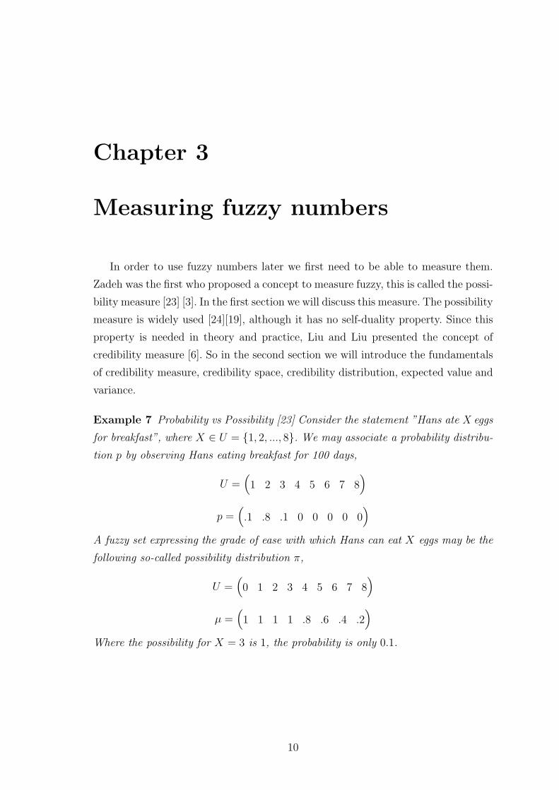
Take for example ξ = (2, 3, 5) and η = (3, 5, 6), then their product is
µ(x) =
14(−7 +
√1 + 8x) if6 ≤ x ≤ 15
14(17−
√49 + 8x) if15 ≤ x ≤ 30
0 otherwise.
Theorem 2.2.1 (Nguyen’s theorem) [16] Let f : X → X be a continuous function
and let A be a fuzzy number. Then
[f(A)]α = f([A]α)
7
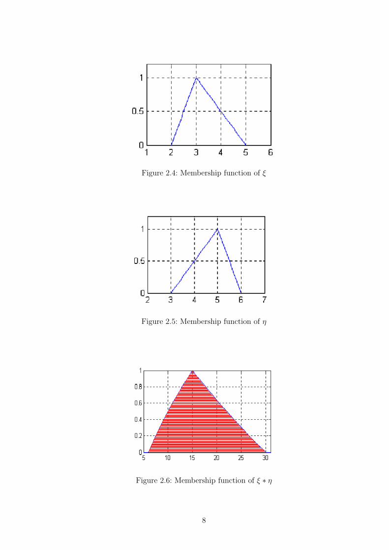
Figure 2.4: Membership function of ξ
Figure 2.5: Membership function of η
Figure 2.6: Membership function of ξ ∗ η
8
where f(A) is defined by the above mentioned extension principle, and
f([A]α) = {f(x) | x ∈ [A]α}.
If [A]α = [a1(α), a2(α)] and f is monotone increasing then we get
[f(A)]α = f([A]α) = f([a1(α), a2(α)]) = [f(a1(α)), f(a2(α))].
Theorem 2.2.2 (Nguyen’s theorem 2.) [16] Let f : X × X → X be a continuous
function and let A and B be fuzzy numbers. Then
[f(A,B)]α = f([A]α, [B]α)
where
f([A]α, [B]α) = {f(x1, x2 | x1 ∈ [A]α, x2 ∈ [B]α)}.
Example 5 (fuzzy max) Let f(x, y) = max{x, y} and let [A]α = [a1(α), a2(α)] and
[B]α = [b1(α), b2(α)] be two fuzzy numbers. Then
[f(A,B)]α = f([A]α, [B]α) = max{[A]α, [B]α} = [a1(α) ∨ b1(α), a2(α) ∨ b2(α)].
Example 6 (fuzzy min) Let f(x, y) = min{x, y} and let [A]α = [a1(α), a2(α)] and
[B]α = [b1(α), b2(α)] be two fuzzy numbers. Then
[f(A,B)]α = f([A]α, [B]α) = min{[A]α, [B]α} = [a1(α) ∧ b1(α), a2(α) ∧ b2(α)].
The fuzzy min and max operations are commutative, associative and distribu-
tive. The distributive property is the following: if A, B and C are fuzzy numbers,
then
max{A,min{B,C}} = min{max{A,B},max{A,C}},
min{A,max{B,C}} = max{min{A,B},min{A,C}}.
9
Chapter 3
Measuring fuzzy numbers
In order to use fuzzy numbers later we first need to be able to measure them.
Zadeh was the first who proposed a concept to measure fuzzy, this is called the possi-
bility measure [23] [3]. In the first section we will discuss this measure. The possibility
measure is widely used [24][19], although it has no self-duality property. Since this
property is needed in theory and practice, Liu and Liu presented the concept of
credibility measure [6]. So in the second section we will introduce the fundamentals
of credibility measure, credibility space, credibility distribution, expected value and
variance.
Example 7 Probability vs Possibility [23] Consider the statement ”Hans ate X eggs
for breakfast”, where X ∈ U = {1, 2, ..., 8}. We may associate a probability distribu-
tion p by observing Hans eating breakfast for 100 days,
U =(1 2 3 4 5 6 7 8
)p =
(.1 .8 .1 0 0 0 0 0
)A fuzzy set expressing the grade of ease with which Hans can eat X eggs may be the
following so-called possibility distribution π,
U =(0 1 2 3 4 5 6 7 8
)µ =
(1 1 1 1 .8 .6 .4 .2
)Where the possibility for X = 3 is 1, the probability is only 0.1.
10
3.1 Possibility measure
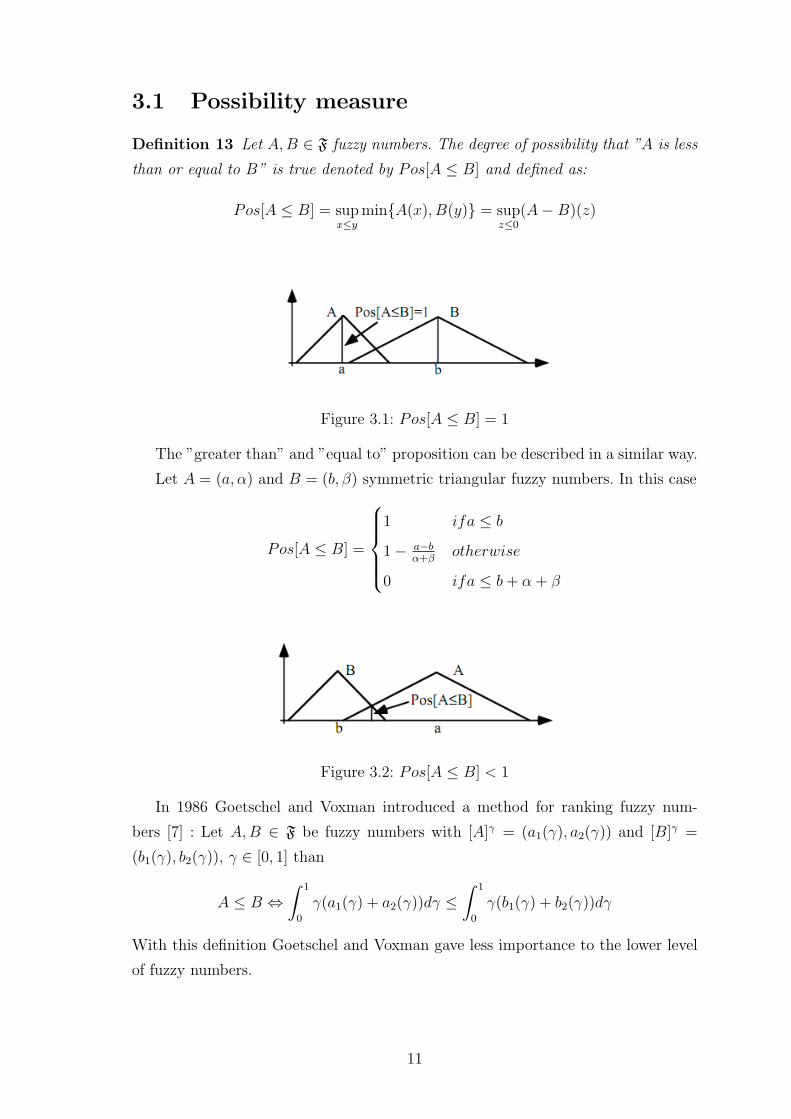
Definition 13 Let A,B ∈ F fuzzy numbers. The degree of possibility that ”A is less
than or equal to B” is true denoted by Pos[A ≤ B] and defined as:
Pos[A ≤ B] = supx≤y
min{A(x), B(y)} = supz≤0
(A−B)(z)
Figure 3.1: Pos[A ≤ B] = 1
The ”greater than” and ”equal to” proposition can be described in a similar way.
Let A = (a, α) and B = (b, β) symmetric triangular fuzzy numbers. In this case
Pos[A ≤ B] =
1 ifa ≤ b
1− a−bα+β
otherwise
0 ifa ≤ b+ α+ β
Figure 3.2: Pos[A ≤ B] < 1
In 1986 Goetschel and Voxman introduced a method for ranking fuzzy num-
bers [7] : Let A,B ∈ F be fuzzy numbers with [A]γ = (a1(γ), a2(γ)) and [B]γ =
(b1(γ), b2(γ)), γ ∈ [0, 1] than
A ≤ B ⇔∫ 1
0
γ(a1(γ) + a2(γ))dγ ≤∫ 1
0
γ(b1(γ) + b2(γ))dγ
With this definition Goetschel and Voxman gave less importance to the lower level
of fuzzy numbers.
11

Definition 14 [2] Using the above mentioned ranking, the possibilistic mean value
of a fuzzy number A can be defined as
E(A) =
∫ 1
0
(a1(γ) + a2(γ))γdγ
Which means that E(A) is the level-weighted average of the arithmetic means of all
γ-level sets.
Example 8 Let A = (a, α, β) be a triangular fuzzy number. Then
[A]γ = [a− (1− γ)α, a+ (1− γ)β], ∀γ ∈ [0, 1]
E(A) =
∫ 1
0
γ[a− (1− γ)α+ a+ (1− γ)β]dγ = a+β − α
6
Definition 15 [2] The possibilistic variance of a fuzzy number A is
V ar(A) = Cov(A,A) =
∫ 1
0
σ2Uγ2γdγ =
1
12
∫ 1
0
(a2(γ)− a1(γ))22γdγ
=1
6
∫ 1
0
(a2(γ)− a1(γ))2γdγ,
where Uγ is a uniform probability distribution on [A]γ and σ2Uγ
denotes the variance
of Uγ
Example 9 Let A = (a, α, β) be a triangular fuzzy number. Then its variance is as
follows:
V ar(A) =1
6
∫ 1
0
γ(a+ β(1− γ)− (a− α(1− γ)))2dγ =
=(α+ β)2
72.
Definition 16 [2] Let A, B are fuzzy numbers. Then their covariance is defined as:
Cov(A,B) =1
2
∫ 1
0
γ(a2(γ)− a1(γ))(b2(γ)− b1(γ))dγ
Example 10 Let A = (a1, α1, β1), B = (a2, α2, β2) be triangular fuzzy numbers.
Then their covariance is:
Cov(A,B) =(α1 + β1)(α2 + β2)
24.
Example 11 Let A = (a, b, c, d) is a trapezoidal fuzzy number. Then the γ-level set,
the expected value and the variance of A is as follows
[A]γ = [a+ γ(b− a), d− γ(d− c)]
E(A) =1
6(a+ d) +
1
3(b+ c)
V (A) =(a− d)2
4+
(c− d+ a− b)2
8+
(d− c)(c− d+ a− b)
3
12
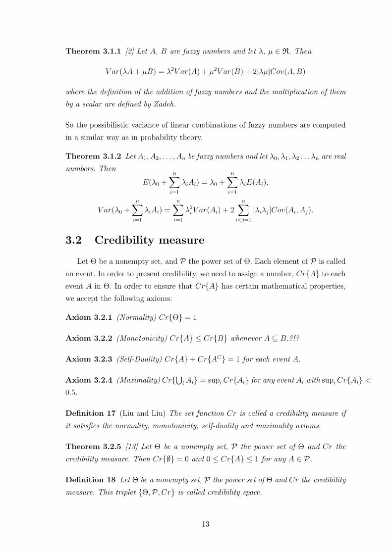
Theorem 3.1.1 [2] Let A, B are fuzzy numbers and let λ, µ ∈ R. Then
V ar(λA+ µB) = λ2V ar(A) + µ2V ar(B) + 2|λµ|Cov(A,B)
where the definition of the addition of fuzzy numbers and the multiplication of them
by a scalar are defined by Zadeh.
So the possibilistic variance of linear combinations of fuzzy numbers are computed
in a similar way as in probability theory.
Theorem 3.1.2 Let A1, A2, . . . , An be fuzzy numbers and let λ0, λ1, λ2 . . . λn are real
numbers. Then
E(λ0 +n∑
i=1
λiAi) = λ0 +n∑
i=1
λiE(Ai),
V ar(λ0 +n∑
i=1
λiAi) =n∑
i=1
λ2iV ar(Ai) + 2
n∑i<j=1
|λiλj|Cov(Ai, Aj).
3.2 Credibility measure
Let Θ be a nonempty set, and P the power set of Θ. Each element of P is called
an event. In order to present credibility, we need to assign a number, Cr{A} to each
event A in Θ. In order to ensure that Cr{A} has certain mathematical properties,
we accept the following axioms:
Axiom 3.2.1 (Normality) Cr{Θ} = 1
Axiom 3.2.2 (Monotonicity) Cr{A} ≤ Cr{B} whenever A ⊆ B.?!?
Axiom 3.2.3 (Self-Duality) Cr{A}+ Cr{AC} = 1 for each event A.
Axiom 3.2.4 (Maximality) Cr{∪
i Ai} = supi Cr{Ai} for any event Ai with supi Cr{Ai} <
0.5.
Definition 17 (Liu and Liu) The set function Cr is called a credibility measure if
it satisfies the normality, monotonicity, self-duality and maximality axioms.
Theorem 3.2.5 [13] Let Θ be a nonempty set, P the power set of Θ and Cr the
credibility measure. Then Cr{∅} = 0 and 0 ≤ Cr{A} ≤ 1 for any A ∈ P.
Definition 18 Let Θ be a nonempty set, P the power set of Θ and Cr the credibility
measure. This triplet {Θ,P, Cr} is called credibility space.
13

Definition 19 A fuzzy variable is defined as a (measurable) function from a credi-
bility space {Θ,P, Cr} to the set of real numbers.
Example 12 Take {Θ,P, Cr} to be {θ1, θ2} with Cr{θ1} = Cr{θ2} = 0.5. Then
the function
ξ(θ) =
0, ifθ = θ1
1, ifθ = θ2
is a fuzzy variable.
Definition 20 Let ξ be a fuzzy variable defined on the credibility space {Θ,P , Cr}.Then its membership function is derived from the credibility measure by
µ(x) = (2Cr{ξ = x}) ∧ 1, x ∈ R.
Membership function represent the degree that the fuzzy variable ξ takes some
prescribed value. The membership degree µ(x) = 0 on if x is an impossible point,
and µ(x) = 1 if x is the most possible point that ξ takes.
Theorem 3.2.6 (Credibility Inversion Theorem) [13] Let ξ be a fuzzy variable with
a membership function µ. Then for any set B of real numbers, we have
Cr{ξ ∈ B} =1
2
(supx∈B
µ(x) + 1− supx∈BC
µ(x)
).
Proof: If Cr{ξ ∈ B} ≤ 0, 5, then by the Monotonicity axiom we have Cr{ξ =
x} ≤ 0, 5 for each x ∈ B. It follows from the Maximality axiom that
Cr{ξ ∈ B} =1
2
(supx∈B
(2Cr{ξ = x} ∧ 1)
)=
1
2supx∈B
µ(x).
The self-duality of credibility measure implies that Cr{ξ ∈ Bc} ≥ 0, 5 and supx∈Bc Cr{ξ =
x} ≥ 0, 5, i.e.,
supx∈Bc
µ(x) = supx∈Bc
(2Cr{ξ = x} ∧ 1) = 1.
It follows from the previous calculations that the statement holds.
If Cr{ξ ∈ B} ≥ 0, 5 then Cr{ξ ∈ Bc} ≤ 0, 5. It follows from the first case that
Cr{ξ ∈ B} = 1− Cr{ξ ∈ Bc} = 1− 1
2
(supx∈Bc
µ(x) + 1− supx∈B
µ(x)
)=
=1
2
(supx∈B
µ(x) + 1− supx∈Bc
µ(x)
).
The theorem is proved.
14
Example 13 Let ξ be a fuzzy variable with a membership function µ. Then the
following equations follow immediately from the Inversion Theorem:
Cr{ξ = x} =1
2
(µ(x) + 1− sup
y =xµ(y)
), ∀x ∈ R;
Cr{ξ ≤ x} =1
2
(supy≤x
µ(y) + 1− supy>x
µ(y)
),∀x ∈ R,
Cr{ξ ≥ x} =1
2
(supy≥x
µ(y) + 1− supy<x
µ(y)
),∀x ∈ R
Theorem 3.2.7 (Sufficient and Necessary Condition for Membership Function)
[13] A function µ : R → [0, 1] is a membership function if and only if supµ(x) = 1.
Proof: If µ is a membership function then there exists a fuzzy variable ξ whose
membership function is just µ, and
supx∈R
µ(x) = supx∈R
(2Cr{ξ = x}) ∧ 1.
If there is some point x ∈ R such that Cr{ξ = x} ≥ 0.5, then supµ(x) = 1.
Otherwise we have Cr{ξ = x} < 0.5 for each q ∈ R. It follows from the Maximality
Axiom that
supx∈R
µ(x) = supx∈R
(2Cr{ξ = x}) ∧ 1 = 2 supx∈R
Cr{ξ = x} = 2(Cr{Θ} ∧ 0.5) = 1.
Conversely, suppose that µ(x) = 1. For each x ∈ R, we define
Cr{x} =1
2
(µ(x) + 1− sup
y =xµ(y)
).
It is clear that
supx∈R
Cr{x} ≥ 1
2(1 + 1− 1) = 0.5.
For any x∗ ∈ R with Cr{x∗} ≥ 0.5, we have µ(x∗) = 1 and
Cr{x∗}+supy =x∗
Cr{y} =1
2
(µ(x∗) + 1− sup
y =x∗µ(y)
)+sup
y =x∗
1
2
(µ(y) + 1− sup
z =yµ(z)
)=
1− 1
2supy =x∗
µ(y) +1
2supy =x∗
µ(y) = 1.
Thus Cr{x} satisfies the credibility extension condition, and has a unique exten-
sion to credibility measure on P(R) by using the credibility extension theorem.
Now we define a fuzzy variable ξ as an identity function from the credibility space
(R,P(R), Cr) to R. Then the membership function of the fuzzy variable ξ is
(2Cr{ξ = x}) ∧ 1 =
(µ(x) + 1− sup
y =xµ(y)
)∧ 1 = µ(x)
for each x. The theorem is proved.
15
Theorem 3.2.8 [13] A fuzzy variable ξ with a membership function µ is (a) non-
negative if and only if µ(x) = 0∀x < 0; (b) positive if and only if µ(x) = 0∀x ≤ 0;
(c) simple if and only if µ takes nonzero values at a finite number of points; (d)
discrete if and only if µ takes nonzero numbers at a countable number of points; (e)
continuous if and only if µ is a continuous function.
3.2.1 Credibility distribution and density function
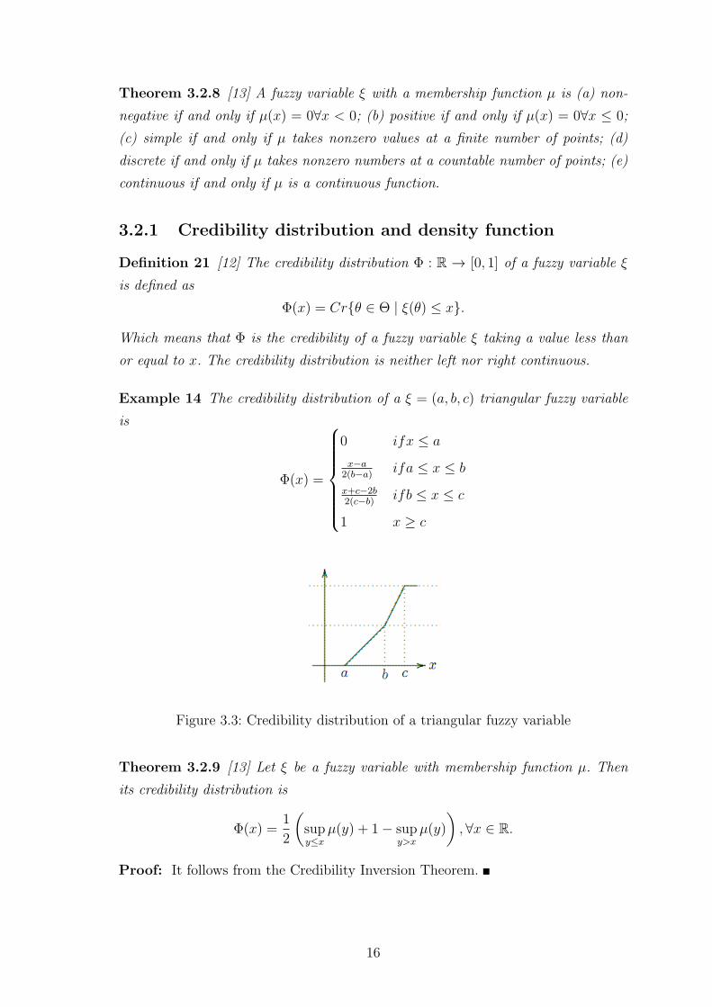
Definition 21 [12] The credibility distribution Φ : R → [0, 1] of a fuzzy variable ξ
is defined as
Φ(x) = Cr{θ ∈ Θ | ξ(θ) ≤ x}.
Which means that Φ is the credibility of a fuzzy variable ξ taking a value less than
or equal to x. The credibility distribution is neither left nor right continuous.
Example 14 The credibility distribution of a ξ = (a, b, c) triangular fuzzy variable
is
Φ(x) =
0 ifx ≤ a
x−a2(b−a)
ifa ≤ x ≤ b
x+c−2b2(c−b)
ifb ≤ x ≤ c
1 x ≥ c
Figure 3.3: Credibility distribution of a triangular fuzzy variable
Theorem 3.2.9 [13] Let ξ be a fuzzy variable with membership function µ. Then
its credibility distribution is
Φ(x) =1
2
(supy≤x
µ(y) + 1− supy>x
µ(y)
),∀x ∈ R.
Proof: It follows from the Credibility Inversion Theorem.
16

Theorem 3.2.10 [11] (Sufficient and Necessary Condition for Credibility Distribu-
tion) A function Φ : R → [0, 1] is a credibility distribution if and only if it is an
increasing function with
limx→−∞
Φ(x) ≤ 0.5 ≤ limx→∞
Φ(x),
limy↓x
ϕ(y) = Φ(x) if limy↓x
Φ(y) > 0.5 or Φ(x) ≥ 0.5
Proof: It is obvious that the credibility distribution Φ is an increasing function.
The first inequalities follow from the credibility asymptotic theorem immediately.
Assume that x is a point at which limy↓z Φ(y) > 0.5. That is,
limy↓z
Cr{ξ ≤ y} > 0.5.
Since {ξ ≤ y} ↓ {ξ ≤ x} as y ↓ x, it follows from the credibility semicontinuity law
that
Φ(y) = Cr{ξ ≤ y} ↓ Cr{ξ ≤ x} = Φ(x)
as y ↓ x. When x is a point at which Φ(x) ≥ 0.5, if limy↓x Φ(y) = Φ(x), then we
have
limy↓x
Φ(y) > Φ(x) ≥ 0.5.
For this case, we have proved that limy↓x Φ(y) = Φ(x). Thus both inequalities are
proved. Conversely, if Φ : R → [q, 1] is an increasing function satisfying the inequal-
ities, then
µ(x) =
2Φ(x), ifΦ(x) < 0.5
1, if limy↑xΦ(y) < 0.5 ≤ Φ(x)
2− 2Φ(x), if0.5 ≤ limy↑x Φ(y)
takes values in [0, 1] and supµ(x) = 1. It follows from the Sufficient and Necessary
Condition for Membership Function Theorem that there is a fuzzy variable ξ whose
membership function is just µ. Let us verify that Φ is the credibility distribution of
ξ, i.e., Cr{ξ ≤ x} = Φ(x) for each x. The argument breaks down into two cases.
(i) If Φ(x) < 0.5, then we have supy>x µ(y) = 1, and µ(y) = 2Φ(y) for each y with
y ≤ x. Thus
Cr{ξ ≤ x} =1
2
(supy≤x
µ(y) + 1− supy>x
µ(y)
)= sup
y≤xΦ(y) = Φ(x).
(ii) If Φ(x) ≥ 0.5, the we have supy≤x µ(y) = 1 and Φ(y) ≥ Φ(x) ≥ 0.5 for each y
with y > x. Thus µ(y) = 2− 2Φ(y) and
Cr{ξ ≤ x} =1
2
(supy≤x
µ(y) + 1− supy>x
µ(y)
)=
1
2
(1 + 1− sup
y>x2− 2Φ(y)
)=
17

= infy>x
Φ(y) = limy↓x
Φ(y) = Φ(x).
The theorem is proved.
Definition 22 (Liu) The credibility density function ϕ : R → [0,+∞) of a fuzzy
variable ξ is a function such that
Φ(x) =
∫ x
−∞ϕ(y)dy, ∀x ∈ R,∫ +∞
−∞ϕ(y)dy = 1
where Φ is the credibility distribution of the fuzzy variable ξ.
Example 15 The credibility density function of a triangular fuzzy variable (a, b, c)
is
ϕ(x) =
1
2(b−a), ifa ≤ x ≤ b
12(c−b)
, ifb ≤ x ≤ c
0 , otherwise.
Example 16 The credibility density function of a trapezoidal fuzzy variable (a, b, c, d)
is
ϕ(x) =
1
2(b−a), ifa ≤ x ≤ b
1d−c
, ifc ≤ x ≤ d
0 , otherwise.
3.2.2 Credibility expected value
For fuzzy numbers there are many ways to define the expected value. The most
accepted definition is given by Liu and Liu. This definition is not only applicable to
continuous fuzzy variables but also discrete ones.
Definition 23 (Liu and Liu) [1] Let ξ be a fuzzy variable. Then the expected value
of ξ is defined by
E[ξ] =
∫ +∞
0
Cr{ξ ≥ r}dr −∫ 0
−∞Cr{ξ ≤ r}dr
provided that at least one of the two integrals is finite.
Theorem 3.2.11 [1] Let ξ be a fuzzy variable with a continuous membership func-
tion µ. If its expected value exists, and there is a point x0 such that µ(x) is increasing
in (−∞, x0) and decreasing in (x0,∞) then its expected value can be calculated as
the following:
E[ξ] = x0 +1
2
∫ +∞
x0
µ(x)dx− 1
2
∫ x0
−∞µ(x)dx.
18

Proof: If x0 ≥ 0, then
Cr{ξ ≥ r} =
12[1 + 1− µ(x)] , if0 ≤ r ≤ x0,
12µ(x) , ifr > x0.
and Cr{ξ ≤ r} = 12µ(x), so we have
E[ξ] =
∫ x0
0
[1− 1
2µ(x)]dx+
∫ ∞
x0
1
2µ(x)dx−
∫ 0
−∞
1
2µ(x)dx =
x0 +1
2
∫ ∞
x0
µ(x)dx− 1
2
∫ x0
−∞µ(x)dx.
The case of x0 < 0 is similar.
Example 17 Let ξ = (a, b, c) be a triangular fuzzy variable. Then its expected value
is
E[ξ] = b+1
2
∫ c
b
x− c
b− cdx− 1
2
∫ b
a
x− a
b− adx =
= b+c− b
4+
a− b
4=
a+ 2b+ c
4.
Example 18 Let ξ = (a, b, c, d) be a trapezoidal fuzzy variable. Then its expected
value is E[ξ] = a+b+c+d4
.
Theorem 3.2.12 (Liu and Liu) [22] Let ξ and η be independent fuzzy variables
with finite expected values. Then for any numbers a and b, we have
E[ξ + b] = E[ξ] + b
E[aξ] = aE[ξ]
E[aξ + bη] = aE[ξ] + bE[η].
Theorem 3.2.13 (Liu) [11] Let ξ be a fuzzy variable whose credibility density func-
tion ϕ exists. If
limx→∞
ϕ(x) = 0, limx→∞
ϕ(x) = 1, and
the Lebesgue integral ∫ +∞
−∞xϕ(x)dx
is finite, then we have
E[ξ] =
∫ +∞
−∞xϕ(x)dx.
Definition 24 (Liu and Liu)[1] Let ξ be a fuzzy variable whose expected value is
finite. Then the variance of ξ is defined by:
V ar[ξ] = E[(ξ − E[ξ])2].
19

Example 19 Let ξ = (a, b, c) be a triangular fuzzy number. Then its variance is:
V ar(ξ) =
∫ +∞
0
Cr{(ξ − E(ξ))2 ≥ x}dx.
We will use our previous knowledge about the expected value of a triangular fuzzy
number:
E(ξ) =a+ 2b+ c
4
to get
Cr{(ξ − E(ξ))2 ≥ x} = Cr{ξ ≥√x+ E(ξ)} =
= Cr
{ξ ≥
√x+
a+ 2b+ c
4
}= Cr{ξ ≥ k} =
=1
2
(supy≥k
µ(y) + 1− supy<k
µ(y)
)=
2 ifk ≤ a
1− 12k−ab−a
ifa < k ≤ b
12k−cb−c
ifb < k ≤ c
0 ifc < k,
where k =√x + a+2b+c
4. Defining α and β, so that α = b − a, β = c − a, we can
continue the previous line as:
=
1 if√x ≤ −3α−β
4
1− 3α+β8α
−√x
2αif −3α−β
4<
√x ≤ α−β
4
3β+α8β
−√x
2βif α−β
4<
√x ≤ α+3β
4
0 if α+3β4
<√x
If we have a symmetric triangular fuzzy number (α = β), then the first two cases
are 0 as well as the last one. So what we have is:
V ar(ξ) =
∫ +∞
0
Cr{(ξ − E(ξ)2) ≥ x}dx =1
2(b− c)
∫ (α+3β4 )
2
0
3β + α
8β−
√x
2βdx =
=1
c− a
∫ ( c−a2 )
2
0
√x− c− a
2dx =
(c− a)2
24.
The non-symmetric case is similar:
V ar[ξ] =
33α3+11αβ2+21α2β−β3
348α, α > β
(c−a)2
24, α = β
33β3+11βα2+21β2α−α3
348β, α < β
Theorem 3.2.14 [13] If ξ is a fuzzy variable whose variance exists, a and b are
real numbers, then V ar[aξ + b] = a2V ar[ξ].
20

Proof: From the definition of variance we get
V [aξ + b] = E[(aξ + b− aE[ξ]− b)2] = a2E[(ξ − E[ξ])2] = a2V [ξ].
21
Chapter 4
Portfolio optimization
The name Markowitz sounds familiar to those working on portfolio selection. His
well-known and widely used mean-variance model used probability theory to chose
between portfolios. In this section we’ll give a short introduction on this model and
turn it into a possibility/credibility model to fit our needs.
4.1 Markowitz model
The fundamental goal of portfolio theory is to optimally allocate your invest-
ments between different assets. Mean variance optimization is a quantitative tool
which will allow you to make this allocation by considering the trade-off between
risk and return. When making investment decision, the investor would always strike
a balance between maximizing the return and minimizing the risk. At the original
Markowitz model the performance of individual securities were considered as ran-
dom variables. The return of the portfolio was quantified as the mean and the return
was quantified as the variance.
In the case of maximizing the return at a given specific level of risk (called the
single period Markowitz mean variance optimization), the standard formulation of
Markowitz model is as follows [15]:
maxE[x1ξ1 + x2ξ2 + . . .+ xnξn]
subject to:
V ar[x1ξ1 + x2ξ2 + . . .+ xnξn] ≤ γ
x1 + x2 + . . .+ xn = 1
xi ≥ 0, i = 1, 2, . . . , n.
, where E denotes the expected value operator, V ar denotes the variance, xi are
22

the investment proportions, in securities i, ξi represents the risk of the i-th security
(i = 1, . . . , n) and γ is the maximum risk level the investor can tolerate.
In this scenario our portfolio will not include short-selling. If short-selling is
allowed, we have to delete the xi ≥ 0.i = 1, 2, . . . , n constraints. Short-selling means
that the investor can sell shares without owning them. This can be done by borrowing
shares from the broker and only reasonable when the prices fall.
Let C be the variance-covariance matrix of the returns as follows:σ11 . . . σ1n
.... . .
...
σn1 . . . σnn
The previous model can be converted into the following, using x = (xi, x2, . . . , xn)
, e = (E[ξ1], E[ξ2], . . . , E[ξn]), and C for the variance-covariance matrix of random
vector of the returns ξ = (ξ1, ξ2, . . . , ξn):
maxxet
subject to:
xCxt ≤ γ∑ni=1 xi = 1
xi ≥ 0, i = 1, 2, . . . , n.
The rates of returns are not necessarily random variables in real life. If we know
historical data for returns of the considered assets, we can calculate the next period’s
return as the mean of the previous returns of one asset.
To get the returns of an asset if only the stock-market prices are given we can
use the following formula: ξi = 100Pi−Pi−1
Pi, where Pi is the price of the asset in the
ith period.
The first approach to solve this constrained maximization problem is to eliminate
(i.e.) xn with the help of the∑n
i=1 xi = 1, and get a problem which includes only
n− 1 unknown parameters.
However, contrary to its theoretical reputation, the Markowitz’s mean-variance
model is not used extensively to construct large-scale portfolios. One of the most
important reasons for this is the computational difficulty associated with solving a
large-scale quadratic programming problem with a dense covariance matrix.
As a basic problem we can consider the Markowitz model’s simpler version where
we are dealing only with the maximization of the return or the minimization of the
risk. If we also include short-selling, we will get the following problems:
23

maxxet
subject to:∑n
i=1 xi = 1
or minxCxt
subject to:∑n
i=1 xi = 1
After eliminating one xi (for example xn) we get a ”simple” n-asset portfolio
optimization problem with n−1 unknown parameters. To eliminate xn, let us define
an n-vector α =(
0 . . . 0 1)
and β =
1 0 . . . 0 −1
0 1 . . . 0 −1...
......
......
0 0 . . . 1 −1
, which is an
(n − 1)xn matrix. Using yi = xi(i = 1, . . . , n − 1), x = α + yβ. And we get the
following:
min(α+ yβ)C(α+ yβ)t
, or for the maximization problem:
max(α+ yβ)et
One way to make the computation easier is to use absolute deviation risk function
instead of the original. This new mean absolute deviation portfolio optimization
model maintain the favorable properties of the Markowitz model, but removes most
of the difficulties of solving it, since it can be reduced to a linear programming
problem.
4.2 Markowitz mean-variance model with fuzzy
returns
In order to use the mean-variance model, it is necessary to estimate the expected
return vector and a covariance matrix. In the original mean-variance model uncer-
tainty of the return is equated with randomness, but it turned out that fuzzy number
is a more powerful tool to describe an uncertain environment. In important cases,
it might be easier to estimate the possibility or credibility distributions of rates of
return on risky assets than the corresponding probability distributions. Based on
these facts, we discuss the portfolio selection problem under the assumption that
the returns of assets are fuzzy numbers.
24

Let’s consider a financial market with n risky assets and a risk-less asset. Let r0
be the interest rate of the risk-less asset. Analogue to the Markowitz mean variance
model the possibilistic/credibilistic mean value is the measure of the investment
return and possibilistic/credibilistic variance is the measure of the investment risk.
4.2.1 Involving fuzzyness into the model
As mentioned before, the rate of return of an asset is calculated from the his-
torical data of the asset with the mean or the median of the previous periods. More
information can be added to our model if we consider including not only the mean
or the variance but a minimum and maximum return of an asset in the selected
period. This can be done with fuzzy numbers. Let us take triangular fuzzy numbers
as returns with the mean (ξ) as peak (a) and ξ − ξmin as α, ξmax − ξ as β.
We will use the following theorems here [19]:
E(λ0 +n∑
i=1
λiAi) = λ0 +n∑
i=1
λiE(Ai),
V ar(λ0 +n∑
i=1
λiAi) =n∑
i=1
λ2iV ar(Ai) + 2
n∑i<j=1
|λiλj|Cov(Ai, Aj),
And the possibilistic mean value, variance and covariance of a triangular fuzzy num-
ber Ai = (ai, αi, βi):
E(A) = a+β − α
6
V ar(A) =(α+ β)2
72
Cov(A1, A2) =(α1 + β1)(α2 + β2)
24
where A1, A2, . . . , An are fuzzy numbers and λ0, λ1, λ2 . . . λn are real numbers.
We get the following optimization problem:
maxn∑
i=1
xi
(ai +
βi − αi
6
)
s.t.
n∑i=1
x2i
(αi + βi)2
72+ 2
n∑i=j=1
(αi + βi)(αj + βj)|xi||xj|24
≤ γ
, which is with the previously defined ai, αi and βi can be transformed into
maxn∑
i=1
ξi,max + ξi,min + 4ξ
6
s.t.
n∑i=1
x2i
(ξi,max − ξi,min)2
72+ 2
n∑i=j=1
(ξi,max − ξi,min)(ξj,max − ξj,min)|xi||xj|24
≤ γ
25
4.2.2 Possibilistic mean-variance with one risk-free asset
Some say that there are no risk-free asset in real life because all assets carry
some degree of risk. However some assets’ (treasuries from the U.S. or from stable
Western governments) level of risk is so small that they can be technically considered
risk-free or risk-less.
Let’s take first the possibilistic approach of the above mentioned mean-variance
model. The general model with n risky and one risk-less asset is the following:
minV ar[ξtx+ ξ0(1− F tx)]
s.t.E[ξtx+ ξ0(1− F tx)] ≥ µ,
x ∈ H
where x = (x1, x2, . . . , xn), r = (r1, r2, . . . , rn), F = (1, 1, . . . , 1) H is a convex set
representing the additional constraints on the choice of x. The return rate of the
jth asset is ξj, and the proportion of total investment to this asset is xj. We use the
prime (t) to denote matrix transposition.
The the possibilistic mean value of the return of the portfolio is given by:
E[ξtx+ ξ0(1− F tx)] = E(n∑
i=1
ξixi) + ξ0(1−n∑
i=1
xi) =
=n∑
i=1
E(ξi)xi + ξ0(1−n∑
i=1
xi) =
=n∑
i=1
(ai +βi − αi
6)xi + ξ0(1−
n∑i=1
xi).
And the corresponding possibilistic variance of the return is:
V ar[ξtx+ξ0(1−F tx)] = V ar[n∑
i=1
ξixi] =1
72
[n∑
i=1
(αi + βi)2x2
i
]+
1
12
n∑i =j=1
(αi+βi)(αj+βj)|xi||xj|
=1
72
[n∑
i=1
(αi + βi)|xi|
]2
.
So the possibilistic mean-variance model can be described by:
min1
72
[n∑
i=1
(αi + βi)2x2
i
]+
1
12
n∑i =j=1
(αi + βi)(αj + βj)|xi||xj|
s.t.n∑
i=1
(ai +βi − αi
6)xi + ξ0(1−
n∑i=1
xi) ≥ µ,
x ∈ H,
26
where H is a convex set representing the additional constraints of x. The previous
model is equal to the following:
min1
72
[n∑
i=1
(αi + βi)2x2
i
]+
1
12
n∑i =j=1
(αi + βi)(αj + βj)|xi||xj|
s.t.n∑
i=1
(ai − ξ0 +βi − αi
6)xi ≥ µ− ξ0,
x ∈ H,
where H is a convex set representing the additional constraints of x.
This model contains only 3n unknown parameters as opposed to the probabilistic
mean-variance model, which contains (n2+3n+2)/2 unknown parameters. We could
further decrease the number of unknown parameters by using symmetric triangular
fuzzy numbers ri = (ai, αi) (αi = βi).
4.2.3 Credibilistic mean-variance with one risk-free asset
The credibilistic model doesn’t differ much from the possibilistic one. Since the
credibilistic variance of triangular fuzzy numbers had three cases, we will consider
only the symmetric one, where the left-width equals the right-width, which means
ξi = (ai, αi), where ai is the peak and αi is the left and right width.
The expected value and variance of a symmetric triangular fuzzy number is
E[ξi] = ai
V ar[ξi] =α2i
6
Since adding two (symmetric) triangular fuzzy numbers also results a triangular
fuzzy number with peak a1 + a2 and left/right width α1 + α2, we have:
E[n∑
i=1
ξi] =n∑
i=1
ai
and
V ar[n∑
i=1
ξi] =
∑ni=1 αi
6.
With other features of the credibilistic expected value, the return of the portfolio x
is
E[ξtx+ ξ0(1− F tx)] = E[n∑
i=1
ξixi] + ξ0(1−n∑
i=1
xi) =
n∑i=1
E[ξi]xi + ξ0(1−n∑
i=1
xi) =n∑
i=1
aixi + ξ0(1−n∑
i=1
xi),
27

and the corresponding credibilistic variance is:
V ar[ξtx+ ξ0(1− F tx)] = V ar[n∑
i=1
ξixi] =(∑n
i=1 xiαi)2
6.
Thus the credibilistic mean-variance model of the portfolio x is given by
min(∑n
i=1 xiα1)2
6
s.t.∑
i = 1naixi + ξ0(1−n∑
i=1
xi) ≥ µ
x ∈ H,
where H is a convex set representing the additional constraints of x.
This problem equals with
minn∑
i=1
xiαi
s.t.
n∑i=1
(ai − ξ0)xi ≥ µ− ξ0
x ∈ H,
where H is a convex set representing the additional constraints of x.
One way to improve this model is to use fuzzy numbers that suit better the
behavior of ’risk’. We can use trapezoidal or even LR-type fuzzy number for this
case.
28
Chapter 5
Mean-variance model with
transaction costs
Transaction cost is one of the main concerns for portfolio managers, since it has
a significant effect on investment strategy. Ignoring them would result inefficient
portfolios. So first let’s have a brief overview of transaction costs.
Investors has to pay a certain amount of money after every investment they make
whether he/she purchases (invest) or sells (disinvest) assets. The transaction cost
associated with the amount of investment of an asset is a non-decreasing concave
function which means that the transaction cost is relatively high when the amount
of fund is small. This can change after a certain point, so beyond a certain amount
of transaction this function turns into a convex function. This happens when the
amount of investment into an asset is large and there’s not enough supply on the
market, so the price will increase which results a convex function.
Let’s have n securities, and xi be the investment proportion in securities i. The
i-th security return is a fuzzy number ξi (it can be defined as ξi = (p′i+di−pi)/pi, i =
1, . . . , n respectively, where p′i is the estimated closing prices of the securities i in
the next year, pi is the closing prices of the securities i at present and di the esti-
mated dividends of the securities i during the coming year). Let α be the maximum
risk level the investor can tolerate, and ci be the transaction cost associated with
the investment into the i-th security. The investor wants to maximize the cost ef-
fected return at a given specific risk level, so his/her problem can be formulated the
following way:
maxE[n∑
i=1
ξixi]−n∑
i=1
ci(xi)
s.t.V ar[n∑
i=1
ξixi] ≤ α
29

n∑i=1
xi = 1
xi ≥ 0, i = 1, . . . , n
5.1 Hybrid intelligent algorithm
Genetic algorithm is considered successful in providing good solutions to many
complex optimization problems, and widely used for solving fuzzy optimization prob-
lems as well. In solving this problem first a fuzzy simulation is applied to compute
the expected value and variance of a fuzzy variable then fuzzy simulation and ge-
netic algorithm are integrated to produce a hybrid intelligent algorithm. With these
we will be able to handle all forms of fuzzy membership functions.
5.1.1 Fuzzy simulation
Fuzzy simulation for credibility: [20] [10] Let ξi be fuzzy variables with
membership functions µi, i = 1, . . . , n. Let x = (x1, . . . , xn), ξ = (ξ1, . . . , ξn) and
µ = (µ1, . . . , µn). Let µ denote the membership function of ξ.
For our model we will need to compute the expected values and variances. Since
V ar[xξ] = E[(xξ − E[xξ])2], therefore computing E[f(xξ)] is enough for us. We
know that E[ξ] =∫∞0
Cr{ξ ≥ r}dr −∫ 0
−∞Cr{ξ ≤ r}dr.The algorithm is the following:
1. Set E = 0.
2. Randomly generate u1j, u2j, . . . , unj from the ϵ-level sets of ξ1, ξ2, . . . , ξn fuzzy
variables. Let’s have uj = (u1j, u2j, . . . , unj), j = 1, . . . , N , where ϵ is a suffi-
ciently small positive number and N is a sufficiently large number.
3. Set a = f(xu1) ∧ f(xu2) ∧ . . . ∧ f(xuN) and
b = f(xu1) ∨ f(xu2) ∨ . . . ∨ f(xuN).
4. Randomly generate r from [a, b].
5. If r ≥ 0, then E := E + Cr{f(xξ) ≥ r}.
6. If r < 0, then E := E − Cr{f(xξ) ≤ r}.
7. Repeat steps from the fourth to the sixth for N times.
8. E[xξ] = a ∨ 0 + b ∧ 0 + E ∗ (b− a)/N.
30

In order to compute E[xξ] by the definition of the credibilistic expected value we
need Cr{xξ ≥ r}, r ≥ 0 and Cr{xξ < r}, r < 0. Let’s denote µ as the membership
function of xξ
Cr{xξ ≥ r} = 12
(supy≥r µ(y) + 1− supy<r µ(y)
). We will randomly generate uij
(j = 1, . . . , N) from the ϵ-level set of ξi, where N is a sufficiently large number. Using
Zadeh’s extension principle we will calculate results from the following formula:
C =1
2( max1≤j≤N
{ min1≤i≤n
{µi(uij)} | xuj ≥ r}+ 1−
max1≤j≤N
{ min1≤i≤n
{µi(uij)} | xuj < r}) :=
=1
2(N + 1−K)
1. j := 1, N =: 0, K := 0.
2. Randomly generate uij from the ϵ-level set of ξi, i = 1, . . . , n, where ϵ is a
sufficiently small number. uj = (u1j, u2j, . . . , unj)
3. Let’s take mj := min1≤i≤n{µi(uij)}.
4. If xuj ≥ r then update N , if not, update K.
5. j := j + 1, and go back to the second step, if j ≤ N .
6. Return 12(N + 1−K).
Fuzzy simulation for possibility: We need the expected value and the vari-
ance to optimize our portfolio, but since in possibility theory they are both obtained
by the following formulas:
E[A] =
∫ 1
0
(a1(γ) + a2(γ))γdγ
V ar(A) =1
6
∫ 1
0
(a2(γ)− a1(γ))2γdγ,
we can use these in our genetic algorithm.
5.1.2 Genetic algorithm
Representation Structure: [20] [10] In order to encode a solution into a chro-
mosome we need a mapping. This mapping between a solution x = (x1, . . . , xn) and
a chromosome V = (v1, . . . , vn) can be the following:
xi =vi
v1 + v2 + . . . vn, i = 1, . . . , n
31
Initialization: Let the number of chromosomes in the population called pop size,
and initialize pop size chromosomes randomly. We generate random point V =
(v1, . . . , vn) in a [0, 1]n hypercube and check its feasibility: V ar[∑n
i=1 vixi] ≤ α.
If it’s feasible we’ll keep it, if not we will regenerate another point from the hyper-
cube until a feasible is obtained. Repeat this process until the initial feasible pop size
chromosomes V1, . . . , Vpop size is generated.
Feasibility means that a chromosome V = (v1, v2, . . . , vn) has to return 1 for
V ar[∑n
i=1 ξivi] ≤ α.
Evaluation function: Evaluation function Eval(V ) is to assign a probability of
reproduction to each chromosome. Chromosomes with higher fitness will have more
chance to produce offspring by using roulette wheel selection.
The most popular evaluation function is the rank-based evaluation function,
which means that among our chromosomes V1, V2, . . . , Vn with the smaller ordinal
number is better. This evaluation function is defined as Eval(Vi) = a(1− a)i−1 for
each i = 1, . . . , n, where a ∈ (0, 1) is a given parameter.
Selection Process: The selection process is based on spinning the roulette wheel
pop size times. In each round one chromosome is selected via the fitness-proportional
selection. (The reason of the roulette-association is because the a proportion of the
original wheel is assigned to each of the possible selection based on their fitness
value.)
Before spinning the wheel we assume use an order relationship among our chro-
mosomes using the their objective value. If two chromosomes have the same objective
value then we’re indifferent between them and we can rearrange them randomly. Now
our pop size chromosomes are arranged from good to bad: V1, . . . , Vpop size (V1 is the
best, Vn is the worst).
We first calculate the cumulative probability for each chromosome Vi:
p0 = 0, pi =i∑
j=1
Eval(Vj), i = 1, . . . , n,
and divide all pi-s by ppop size, so that ppop size = 1. Note, that i = 1 means the best
individual and i = n is the worst.
Generate a random number r ∈ (0, 1], and select a chromosome Vi such that
pi−1 < r ≤ pi. Repeat the last two steps pop size times, so then we have pop size
copies of chromosomes. Note, that the ’best’ chromosome has more chance to rep-
resent itself in our selection.
Crossover Operation: Primary operations exist for modifying structures in
genetic algorithms. One of them is the crossover operation, in which two chromo-
somes (later called parents) are combined to from two new solutions. The parents
32
are chosen by the following method:
Let’s take a probability parameter Pc for showing the expected amount of chro-
mosomes going through the crossover operation (Pc ∗ pop size), and generate a
random r from (0, 1) pop size times. Vi will be selected as a parent if r < Pc at the
i-th selection of r. After this we have the parents: V ′1 , V
′2 , . . ., and we simply make
couples with pairing them: (V ′1 , V
′2), (V
′3 , V
′4), . . ..
The crossover will look like this: Let’s take a couple, e.g. (V ′1 , V
′2), and generate
a random number s from (0, 1). Then the two children of the couple will be X, Y ,
such that:
X = sV ′1 + (1− s)V ′
2 , Y = (1− s)V ′1 + sV ′
2 .
If the feasible set is convex, then both children will be in the feasible set. If not, we
can still check feasibility of a chromosome. If both children are feasible, we replace
the parents with them. If not, we keep the feasible one (if it exist), and redo the
process of crossover by generating a new s until we obtain two feasible children, or
a given number of cycles is finished.
Mutation This is another way to modify structures in genetic algorithm. Mu-
tation can result new chromosomes, preventing the population from stagnating.
Let’s have a probability parameter Pm for showing the expected number of
chromosomes going through the process of mutation. This number is Pm ∗ pop size.
We generate a random q from (0,1) pop size times, and select Vi as a parent of
a mutation if the actual q < Pm.
For each selected parent V = (v1, v2, . . . , vn) the mutation will be the following:
Let M be a large positive number. We randomly choose a mutation direction
d ∈ Rn. If V + M ∗ d is feasible, we replace the child with its parent (the child
will be part of the next population). If it’s not feasible then we set M as a random
number between 0 and M , until it’s feasible. If we can not find a feasible mutation
of a parent in a predetermined number of iterations, then we set M = 0.
Hybrid Intelligent Algorithm The hybrid intelligent algorithm will terminate
after a given number of cycles. The steps will be the following:
1. Fuzzy simulation and initializing pop size chromosomes.
2. Update the chromosomes by crossover and mutation, in which fuzzy simulation
will be used.
3. Calculate the objective values for the chromosomes (E[∑n
i=1 ξixi]−∑n
i=1 ci(xi))
4. Compute the fitness of each chromosome with the objective values.
5. Spinning the roulette wheel for selecting chromosomes.
33

6. Repeat steps from the second to the fifth for a given number of cycles.
7. Encode best chromosome to get the solution of the portfolio selection.
34

Bibliography
[1] Liu B. and Liu YK. Expected value of fuzzy variable and fuzzy expected value models.
IEEE Transactions on Fuzzy Systems, Vol.10, No.4.
[2] Christer Carlsson and Robert Fuller. Some applications of possibilistic mean value,
variance, covariance and correlation. Technical report.
[3] Christer Carlsson and Robert Fuller. On possibilistic mean value and variance of
fuzzy numbers. Fuzzy Sets and Systems, pages 315–326, 2001.
[4] Peter Majlender Christer Carlsson, Robert Fuller. A possibilistic approach to selecting
portfolios with highest utility score. Fuzzy Sets and Systems, pages 13–21, 2002.
[5] Bogdana Pop Cristinca Fulga. Single period portfolio optimization with fuzzy trans-
action costs. Technical report.
[6] Robert Fuller. Fuzzy reasoning and fuzzy optimization. 1998.
[7] R. Goetschel and W. Voxman. Elementary fuzzy calculus. Fuzzy Sets and Systems,
pages 31–43, 1986.
[8] Xiaoxia Huang. Credibility based portfolio selection. Technical report, University of
Science and Technology Beijing - School of Management, 2006.
[9] Xiaoxia Huang. Portfolio selection with fuzzy returns. Journal of intelligent and fuzzy
systems, pages 283–390, 2007.
[10] John R. Koza. Genetic Programming. MIT, 1994.
[11] Baoding Liu. Uncertainty Theory. Springer-Verlag, 2004.
[12] Baoding Liu. Theory and Practice of Uncertain Programming. Utlab, 2007.
[13] Baoding Liu. Uncertainty Theory. Utlab, 2007.
[14] Elena Almaraz Luengo. Fuzzy mean-variance portfolio selection problems. Advanced
Modeling and Optimization.
[15] Harry Markowitz. Portfolio selection. The Journal of Finance, pages 77–91, 1952.
35
[16] H. T. Nguyen. A note on the extension principle for fuzzy sets. Journal of Mathe-
matical Analysis and Applications.
[17] Zaiyue Zhang Shang Gao. Multiplication operation on fuzzy numbers. Journal of
Software, pages 331–338, 2009.
[18] Hiroaki Ishii Takashi Hasuike. Portfolio selection problems considering fuzzy returns
of future scenarios. Technical report, Osaka University.
[19] Hai-Lin Lan Wei-Guo Zhang, Qianqin Chen. A portfolio selection method based on
possibility theory. Lecture notes on computer science, pages 364–374, 2006.
[20] Hau-San WongZhongfeng Qin Xiang Li, Yang Zhang. A hybrid intelligent algorithm
for portfolio selection problem with fuzzy returns. Journal of Computational and
Applied Mathematics, 2009.
[21] Shou-Yang Wang Yang Fang, K. K. Lai. Portfolio rebalancing model with transaction
costs based on fuzzy decision theory. European Journal of Operational Research.
[22] Liu Yk and Liu B. Expected value operator of random fuzzy variable and random
fuzzy expected value models. International Journal of Uncertainty, Fuzzyness and
Knowledge-Based Systems, Vol. 11, No.2.
[23] L. A. Zadeh. Fuzzy sets. 1965.
[24] Wei-Guo Zhang and Ying-Luo Wang. Notes on possibilistic variances of fuzzy num-
bers. Applied Mathematics Letters, 2007.
[25] Fanji Tian Zhigang Wang. A note of the expected value and variance of fuzzy vari-
ables. International Journal of Nonlinear Science, pages 486–492, 2009.
36