portland communitportland community collegey...
TRANSCRIPT

Portland Community CollegePortland Community CollegeMTH 251 Laboratory ManualMTH 251 Laboratory Manual

Portland Community College MTH 251 Lab Manual
P r e f a c e | i
Table of Contents Rates of Change (Activities 1-3)
Lab Activities Pages 1 – 6 Supplementary Exercises (E1) Pages A1 – A2 (Appendix A) Supplementary Solutions (E1) Pages D1 – D4 (Appendix D)
Limits and Continuity (Activities 4-16)
Lab Activities Pages 7 - 24 Supplementary Graphs Pages B1 - B2 (Appendix B) Limit Laws and Rational Limit Forms Pages C1 – C4 (Appendix C) Supplementary Exercises (E2) Pages A3 – A6 (Appendix A) Supplementary Solutions (E2) Pages D5 – D10 (Appendix D)
Introduction to the First Derivative (Activities 17-20)
Lab Activities Pages 25 - 32 Supplementary Exercises (E3) Pages A7 – A8 (Appendix A) Supplementary Solutions (E3) Pages D11 – D14 (Appendix D)
Functions, Derivatives, and Antiderivatives (Activities 21-26)
Lab Activities Pages 33 - 46 Supplementary Graph Page B3 (Appendix B) Supplementary Exercises (E4) Pages A9 – A14 (Appendix A) Supplementary Solutions (E4) Pages D15 – D18 (Appendix D)
Derivative Formulas (Activities 27-37)
Lab Activities Pages 47 - 56 Rules of Differentiation Pages C5 – C6 (Appendix C) Supplementary Exercises (E5) Pages A15 – A18 (Appendix A) Supplementary Solutions (E5) Pages D19 – D28 (Appendix D)
The Chain Rule (Activities 38-41)
Lab Activities Pages 57 - 62 Rules of Differentiation Pages C5 – C6 (Appendix C) Supplementary Exercises (E6) Pages A19 – A20 (Appendix A) Supplementary Solutions (E6) Pages D29 – D36 (Appendix D)

Portland Community College MTH 251 Lab Manual
ii | P r e f a c e
Implicit Differentiation (Activities 42-43)
Lab Activities Pages 63 - 66 Rules of Differentiation Pages C5 – C6 (Appendix C) Supplementary Exercises (E7) Pages A21 – A22 (Appendix A) Supplementary Solutions (E7) Pages D37 – D40 (Appendix D)
Related Rates (Activities 44-47)
Lab Activities Pages 67 - 72 Supplementary Exercises (E8) Pages A23 – A24 (Appendix A) Supplementary Solutions (E8) Pages D41 – D44 (Appendix D)
Critical Numbers and Graphing from Formulas (Activities 48-54)
Lab Activities Pages 73 - 84 Supplementary Exercises (E9) Pages A25 – A26 (Appendix A) Supplementary Solutions (E9) Pages D45 – D53 (Appendix D)

Portland Community College MTH 251 Lab Manual
P r e f a c e | iii
To the Student MTH 251 is taught at Portland Community College using a lecture/lab format. The laboratory time is set aside for students to investigate the topics and practice the skills that are covered during their lecture periods. The lab activities have been written under the presumption that students will be working in groups and will be actively discussing the examples and problems included in each activity. Many of the exercises and problems lend themselves quite naturally to discussion. Some of the more algebraic problems are not so much discussion problems as they are “practice and help” problems. You do not need to fully understand an example before starting on the associated problems. The intent is that your understanding of the material will grow while you work on the problems. When working through the lab activities the students in a given group should be working on the same activity at the same time. Sometimes this means an individual student will have to go a little more slowly than he or she may like and sometimes it means an individual student will need to move on to the next activity before he or she fully grasps the current activity. Many instructors will want you to focus some of your energy on the way you write your mathematics. It is important that you do not rush through the activities. Write your solutions as if they are going to be graded; that way you will know during lab time if you understand the proper way to write and organize your work. If your lab section meets more than once a week, you should not work on lab activities between lab sections that occur during the same week. It is OK to work on lab activities outside of class once the entire classroom time allotted for that lab has passed. There are not written solutions for the lab activity problems. Between your group mates, your instructor, and (if you have one) your lab assistant, you should know whether or not you have the correct answers and proper writing strategies for these problems. Each lab has a section of supplementary exercises; these exercises are fully keyed. The supplementary exercises are not simply copies of the problems in the lab activities. While some questions will look familiar, many others will challenge you to apply the material covered in the lab to a new type of problem. These questions are meant to supplement your textbook homework, not replace your textbook homework.
The MTH 251 Laboratory Manual was written by Steve Simonds.
The cover art for the manual was designed by Phil Thurber.
The cover includes a page from Isaac Newton’s Philosophiæ Naturalis Principia Mathematica.
The cover includes William Blake’s “Newton.”

Portland Community College MTH 251 Lab Manual
iv | P r e f a c e
To the Instructor This manual is significantly different from earlier versions of the lab manual. The topics have been arranged in a developmental order. Because of this, students who work each activity in the order they appear may not get to all of the topics covered in a particular week. It is strongly recommended that the instructor pick and choose what they consider to be the most vital activities for a given week and that the instructor have the students work those activities first; for some activities you might also want to have the students only work selected problems in the activity. Students who complete the high priority activities and problems can then go back and work the activities that they initially skipped. There are also fully keyed problems in the supplementary exercises that the students could work on both during lab time and outside of class. A suggested schedule for the labs is shown in Table P1. Again, the instructor should choose what they feel to be the most relevant activities and problems for a given week and have the students work those activities and problems first.
Table P1: Possible 10 week schedule for the labs. (Students should consult their syllabus for their schedule.)
Week Labs (Lab Activities) Supplementary Exercises
1 Rates of Change/Limits and Continuity (1-4) E1 (all)
2 Limits and Continuity (5-16) E2 (all)
3 Introduction to the First Derivative (17-20) E3 (all)
4 Functions, Derivatives, and Antiderivatives (21-24) E4.1-E4.5
5 Functions, Derivatives, and Antiderivatives (25-26) E4.6-E4.10
6 Derivative Formulas (27-37) E5 (all)
7 The Chain Rule (38-41) E6 (all)
8 Implicit Differentiation/Related Rates (42-47) E7 (all), E8 (all)
9 and 10 Critical Numbers and Graphing from Formulas (48-54) E9 (all)

Portland Community College MTH 251 Lab Manual
L a b A c t i v i t i e s | 1
Rates of Change Activity 1
Motion is frequently modeled using calculus. A building block for this application is the concept of average velocity. Average velocity is defined to be net displacement divided by elapsed time. More precisely, if p is a position function for something moving along a numbered line, then we define the average velocity over the time interval 0 1,t t to be:
Expression 1.1: 1 0
1 o
p t p t
t t
Problem 1.1 According to simplified Newtonian physics, if an object is dropped from a height of 200 m and allowed to freefall to the ground, then the height of the object (measure in m) is given by the position function 2200 4.9p t t where t is the amount of time that has passed since the
object was dropped (measured in s).
1.1.1 What, including unit, are the values of p t three seconds and five seconds into the
object’s fall? Use these values when working problem 1.1.2.
1.1.2 Calculate 5s 3 s
5 s 3 sp p
; include units while making the calculation. What does the
result tell you in the context of this problem?
1.1.3 Use Expression 1.1 to find a formula for the average velocity of this object over the general time interval 0 1,t t . The first couple of lines of this process are shown below. Copy these lines onto your paper and continue the simplification process.
2 21 01 0
1 0 1 02 2
1 0
1 02 2
1 0
1 0
200 4.9 200 4.9
200 4.9 200 4.9
4.9 4.9
t tp t p t
t t t t
t t
t t
t t
t t
1.1.4 Check the formula you derived in problem 1.1.3 using 0 3t and 1 5t ; that is, compare the value generated by the formula to that you found in problem 1.1.2.
1.1.5 Using the formula found in problem 1.1.3, replace
0t with 3 but leave 1t as a variable; simplify the result. Then copy Table 1.1 onto your paper and fill in the missing entries.
Table 1.1: 1
1
33
p t py
t
1t (s) y (m/s) 2.9 2.99 2.999 3.001 3.01 3.1
Hint
In the next step you should factor 4.9 from the numerator; the remaining factor will factor further.

Portland Community College MTH 251 Lab Manual
2 | L a b A c t i v i t i e s
1.1.6 As the value of 1t gets closer to 3 , the values in the y column of Table 1.1 appear to be converging on a single number; what is this number and what do you think it tells you in the context of this problem?
Activity 2
One of the building blocks in differential calculus is the secant line to a curve. It is very easy for a line to be considered a secant line to a curve; the only requirement that must be fulfilled is that the line intersects the curve in at least two points.
In Figure 2.1, a secant line to the curve y f x has been
drawn through the points 0,3 and 4, 5 . You should verify
that the slope of this line is 2 .
The formula for f is 23 2f x x x . We can use this
formula to come up with a generalized formula for the slope of secant lines to this curve. Specifically, the slope of the line connecting the point 0 0,x f x to the point 1 1,x f x is
derived in Example 2.1.
Example 2.1
1 0sec
1 0
2 21 1 0 0
1 02 2
1 1 0 0
1 0
2 21 0 1 0
1 0
1 0 1 0 1 0
1 0
1 0 1 0
1 0
1 0 1 0
3 2 3 2
3 2 3 2
2 2
2
2
2 for
f x f xm
x x
x x x x
x x
x x x x
x x
x x x x
x x
x x x x x x
x x
x x x x
x x
x x x x
We can check our formula using the line in Figure 2.1. If we let 0 0x and 1 4x then our simplified slope formula gives us:
1 02 2 4 02
x x
This factoring technique is called factoring by grouping.
Figure 2.1: f

Portland Community College MTH 251 Lab Manual
L a b A c t i v i t i e s | 3
Problem 2.1
Let 2 5g x x . 2.1.1 Following Example 2.1, find a formula for the slope of the
secant line connecting the points 0 0,x g x and
1 1,x g x . Please note that factoring by grouping will
not be necessary when simplifying the expression,
2.1.2 Check your slope formula using the two points indicated in Figure 2.2. That is, use the graph to find the slope between the two points and then use your formula to find the slope; make sure that the two values agree!
Activity 3
While it’s easy to see that the formula 1 0
1 0
f x f x
x x
gives the slope of the line connecting two
points on the function f, the resultant expression can at times be awkward to work with. We actually already saw that when we had to use slight-of-hand factoring in Example 2.1. The algebra associated with secant lines (and average velocities) can sometimes be simplified if we designate the variable h to be the run between the two points (or the length of the time interval). With this designation we have 1 0x x h which gives us 1 0x x h . Making these substitutions we get Equation 3.1. The expression on the right side of Equation 3.1 is called the difference quotient for f.
Equation 3.1 1 0 0 0
1 0
f x f x f x h f x
x x h
Let’s revisit the function 23 2f x x x from Example 2.1. The difference quotient for this
function is derived in Example 3.1.
Example 3.1
2 20 0 0 00 0
2 2 20 0 0 0 0
20
0
0
3 2 3 2
3 2 2 2 3 2
2 2
2 2
2 2 for 0
x h x h x xf x h f x
h h
x h x x h h x x
h
h x h h
hh x h
hx h h
Figure 2.2: g

Portland Community College MTH 251 Lab Manual
4 | L a b A c t i v i t i e s
Please notice that all of the terms without a factor of h subtracted to zero. Please notice, too, that we avoided all of the tricky factoring that appeared in Example 2.1! For simplicity’s sake, we generally drop the variable subscript when applying the difference quotient. So for future reference we will define the difference quotient as follows:
Problem 3.1 Completely simplify the difference quotient for each of the following functions. Please note that the template for the difference quotient needs to be adapted to the function name and independent variable in each given equation. For example, the difference quotient for the function
in problem 3.1.1 is v t h v t
h
.
Please make sure that you lay out your work in a manner consistent with the way the work is shown in example 3.1 (excluding the subscripts, of course).
3.1.1 22.5 7.5v t t t 3.1.2 3 7g x x 3.1.3 32
w xx
Problem 3.2 Suppose that an object is tossed into the air in such a way that the elevation of the object (measured in ft) is given by the function 240 40 16s t t t where t is the amount of time that
has passed since the object was tossed (measured in s). 3.2.1 Simplify the difference quotient for s.
3.2.2 Ignoring the unit, use the difference quotient to determine the average velocity over the interval 1.6,2.8 . (Hint: Use 1.6t and 1.2h . Make sure that you understand why!)
3.2.3 What, including unit, are the values of 1.6s and 2.8s ? Use these values when working
problem 3.2.4.
3.2.4 Use the expression 2.8 1.6
2.8 1.6s s
to verify the value you found in problem 3.2.2. Include
the unit while making this calculation. 3.2.5 Ignoring the unit, use the difference quotient to determine the average velocity over the
interval 0.4,2.4 .
Definition 3.1
The difference quotient for the function y f x is the expression f x h f x
h
.

Portland Community College MTH 251 Lab Manual
L a b A c t i v i t i e s | 5
Problem 3.3
Moose and squirrel were having casual conversation when suddenly, without any apparent provocation, Boris Badenov launched anti-moose missile in their direction. Fortunately, squirrel had ability to fly as well as great knowledge of missile technology, and he was able to disarm missile well before it hit ground.
The elevation (ft) of the tip of the missile t seconds after it was launched is given by the function 216 294.4 15h t t t .
3.3.1 What, including unit, is the value of 12h and what does the value tell you about the flight
of the missile?
3.3.2 What, including unit, is the value of 10 s 0 s
10 sh h
and what does this value tell you
about the flight of the missile?
3.3.3 The velocity (ft/s) function for the missile is 32 294.4v t t . What, including unit, is
the value of 10 s 0 s
10 sv v
and what does this value tell you about the flight of the
missile?
Problem 3.4
Timmy lived a long life in the 19th century. When Timmy was seven he found a rock that weighed exactly half a stone. (Timmy lived in jolly old England, don’t you know.) That rock sat on Timmy’s window sill for the next 80 years and wouldn’t you know the weight of that rock did not change even one smidge the entire time. In fact, the weight function for this rock was 0.5w t where w t
was the weight of the rock (stones) and t was the number of years that had passed since that day Timmy brought the rock home. 3.4.1 What was the average rate of change in the weight of the rock over the 80 years it sat on
Timmy’s window sill?
3.4.2 Ignoring the unit, simplify the expression 1 0
1 0
w t w t
t t
. Does the result make sense in
the context of this problem?
3.4.3 Showing each step in the process and ignoring the unit, simplify the difference quotient for w . Does the result make sense in the context of this problem?

Portland Community College MTH 251 Lab Manual
6 | L a b A c t i v i t i e s
Problem 3.5
Truth be told, there was one day in 1842 when Timmy’s mischievous son Nigel took that rock outside and chucked it into the air. The velocity of the rock (ft/s) was given by 60 32v t t
where t was the number of seconds that had passed since Nigel chucked the rock. 3.5.1 What, including unit, are the values of 0v , 1v , and 2v and what do these values tell
you in the context of this problem? Don’t just write that the values tell you the velocity at certain times; explain what the velocity values tell you about the motion of the rock.
3.5.2 Ignoring the unit, simplify the difference quotient for v .
3.5.3 What is the unit for the difference quotient for v ? What does the value of the difference quotient (including unit) tell you in the context of this problem?
Problem 3.6 Suppose that a vat was undergoing a controlled drain and that the amount of fluid left in the vat (gal) was given by the formula 3/2100 2V t t where t is the number of minutes that had
passed since the draining process began. 3.6.1 What, including unit, is the value of 4V and what does that value tell you in the context
of this problem?
3.6.2 Ignoring the unit, write down the formula you get for the difference quotient of V when 4t . Copy Table 3.1 onto your paper and fill in the missing values. Look for a pattern in the output and write down enough digits for each entry so that the pattern is clearly illustrated ; the first two entries in the output column have been given to help you understand what is meant by this direction.
3.6.3 What is the unit for the y values in Table 3.1? What do these values (with their unit) tell you in the context of this problem?
3.6.4 As the value of h gets closer to 0 , the values in the y column of Table 3.1 appear to be converging to a single number; what is this number and what do you think that value (with its unit) tells you in the context of this problem?
Table 3.1: 4 4V h V
yh
h y 0.1 5.962 0.01 5.9962 0.001 0.001 0.01 0.1

Portland Community College MTH 251 Lab Manual
L a b A c t i v i t i e s | 7
Limits and Continuity Activity 4 While working problem 3.6 you completed Table 4.1 (formerly Table 3.1). In the context of that problem the difference quotient being evaluated returned the average rate of change in the volume of fluid remaining in a vat between times 4t and 4t h . As the elapsed time closes in on 0 this average rate of change converges to 6 . From that we deduce that the rate of change in the volume 4 minutes into the draining process must have been 6 gal/min. Please note that we could not deduce the rate of change 4 minutes into the process by replacing h with 0 ; in fact, there are at least two things preventing us from doing so. From a strictly mathematical perspective, we cannot replace h with 0 because that would lead to division by zero in the difference quotient. From a more physical perspective, replacing h with 0 would in essence stop the clock. If time is frozen, so is the amount of fluid in the vat and the entire concept of “rate of change” becomes moot. It turns out that it is frequently more useful (not to mention interesting) to explore the trend in a function as the input variable approaches a number rather than the actual value of the function at that number. Mathematically we describe these trends using limits. If we call the difference quotient in the heading for Table 4.1 f h , then we could describe the
trend evidenced in the table by saying “the limit of f h as h approaches zero is 6 .” Please note
that as h changes value, the value of f h changes, not the value of the limit. The limit value is a
fixed number to which the value of f h converges. Symbolically we write 0
lim 6h
f h
Most of the time the value of a function at the number a and the limit of the function as x approaches a are in fact the same number. When this occurs we say that the function is continuous at a . However, to help you better understand the concept of limit we need to have you confront situations where the function value and limit value are not equal to one another. Graphs can be useful for helping distinguish function values from limit values, so that is the perspective you are going to use in the first couple of problems in this lab.
Table 4.1: 4 4V h V
yh
h y 0.1 5.962 0.01 5.9962 0.001 5.99962 0.001 6.00037 0.01 6.0037 0.1 6.037
The context for Problem 3.6 Suppose that a vat was undergoing a controlled drain and that the amount of fluid left in the vat (gal) was given by the formula 3/2100 2V t t
where t is the number of minutes that had passed since the draining process began.

Portland Community College MTH 251 Lab Manual
8 | L a b A c t i v i t i e s
Problem 4.1 Several function values and limit values for the function in Figure 4.1 are given below. You and your group mates should take turns reading the equations aloud. Make sure that you read the symbols correctly, that’s part of what you are learning! Also, discuss why the values are what they are and make sure that you get help from your instructor to clear up any confusion.
2 6f but 2
lim 3x
f x
4f is undefined but 4
lim 2x
f x
1 1f but 1
limx
f x
does not exist
1
lim 3x
f x
but 1
lim 1x
f x
Problem 4.2 Copy each of the following expressions onto your paper and either state the value or state that the value is undefined or doesn’t exist. Make sure that when discussing the values you use proper terminology. All expressions are in reference to the function g shown in Figure 4.2. 4.2.1 5g 4.2.2
5limt
g t
4.2.3 3g
4.2.4 3
limt
g t
4.2.5 3
limt
g t
4.2.6 3
limt
g t
4.2.7 2g 4.2.8 2
limt
g t
4.2.9 2g
4.2.10 2
limt
g t
4.2.11 2
limt
g t
4.2.12 2
limt
g t
The limit of f x as x approaches 1 from the left.
The limit of f x as x approaches 1 from the right.
Figure 4.1: f
Figure 4.2: g

Portland Community College MTH 251 Lab Manual
L a b A c t i v i t i e s | 9
Problem 4.3
Values of the function 2
2
3 16 52 13 15
x xf x
x x
are shown
in Table 4.2. Both of the questions below are in reference to this function. 4.3.1 What is the value of 5f ?
4.3.2 What is the value of 2
25
3 16 5lim2 13 15x
x x
x x
?
Problem 4.4
Values of the function 12p t t are shown in Table
4.3. Both of the questions below are in reference to this function. 4.4.1 What is the value of 21p ?
4.4.2 What is the value of 21
lim 12t
t
?
Problem 4.5
Create tables similar to tables 4.2 and 4.3 from which you can deduce each of the following limit values. Make sure that you include table numbers, table captions, and meaningful column headings. Make sure that your input values follow patterns similar to those used in tables 4.2 and 4.3. Make sure that you round your output values in such a way that a clear and compelling pattern in the output is clearly demonstrated by your stated values. Make sure that you state the limit value!
4.5.1 2
6
10 24lim6t
t t
t
4.5.2
1
sin 1lim
3 3x
x
x
4.5.3 0
lim4 16h
h
h
Activity 5 When proving the value of a limit we frequently rely upon laws that are easy to prove using the technical definitions of limit. These laws can be found in Appendix C (pages C1 and C2). The first of these type laws are called replacement laws. Replacement laws allow us to replace limit expressions with the actual values of the limits. Problem 5.1 The value of each of the following limits can be established using one of the replacement laws. Copy each limit expression onto your own paper, state the value of the limit (e.g.
9lim 5 5x
), and state
the replacement law (by number) that establishes the value of the limit.
5.1.1 limt
t
5.1.2 14lim 14x
5.1.3 14limx
x
Table 4.2: 2
2
3 16 52 13 15
x xf x
x x
x f (x)
4.99 2.0014 4.999 2.00014 4.9999 2.000014 5.0001 1.999986 5.001 1.99986 5.01 1.9986
Table 4.3: 12p t t
t p(t)
20.9 2.98 20.99 2.998 20.999 2.9998 21.001 3.0002 21.01 3.002 21.1 3.02

Portland Community College MTH 251 Lab Manual
10 | L a b A c t i v i t i e s
Problem 5.2 The algebraic limit laws allow us to replace limit expressions with equivalent limit expressions. When applying limit laws our first goal is to come up with an expression in which every limit in the expression can be replaced with its value based upon one of the replacement laws. This process is shown in example 5.1. Please note that all replacement laws are saved for the second to last step and that each replacement is explicitly shown. Please note also that each limit law used is referenced by number.
Example 5.1
2 2
7 7 7
2
7 7
2
7 7
2
lim 4 3 lim 4 lim 3 Limit Law A1
4 lim lim 3 Limit Law A3
4 lim lim 3 Limit Law A6
4 7 3 Limit Laws R1 and R2199
x x x
x x
x x
x x
x
x
Use the limit laws to establish the value of each of the following limits. Make sure that you use the step-by-step, vertical format shown in example 5.1. Make sure that you cite the limit laws used in each step. To help you get started, the steps necessary in problem 5.2.1 are outlined below.
5.2.1 4
lim 6 1t
t
5.2.2 7
3lim9y
y
y y
5.2.3 lim cosx
x x
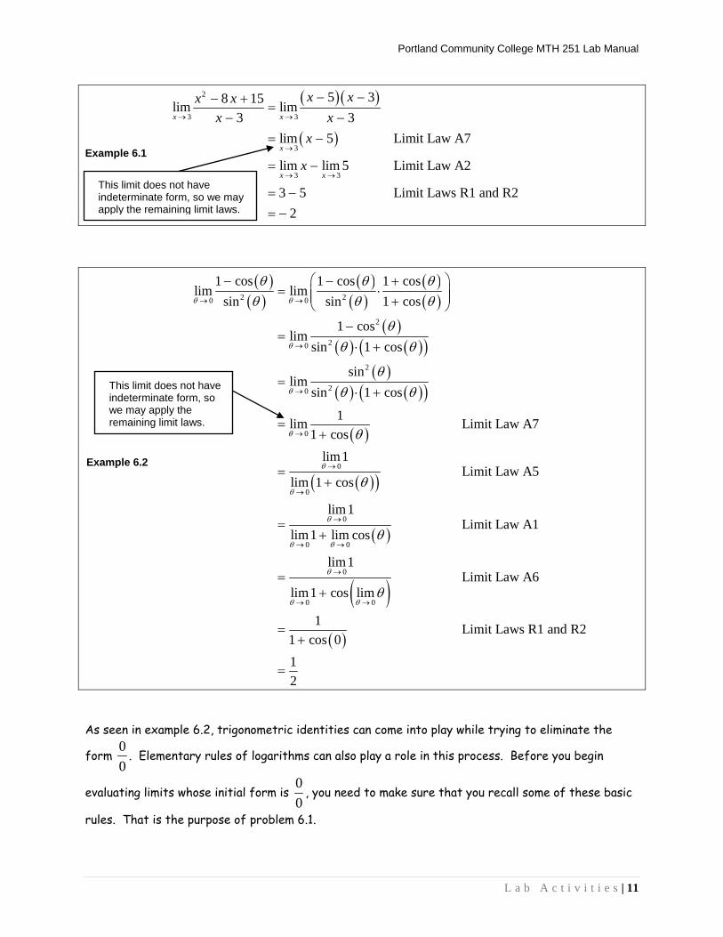
Activity 6
Many limits have the form 00
which means the expressions in both the numerator and denominator
limit to zero (e.g. 3
2 6lim3x
x
x
). The form 00
is called indeterminate because we do not know the
value of the limit (or even if it exists) so long as the limit has that form. When confronted with
limits of form 00
we must first manipulate the expression so that common factors causing the zeros
in the numerator and denominator are isolated. Limit law A7 can then be used to justify eliminating the common factors and once they are gone we may proceed with the application of the remaining limit laws. Examples 6.1 and 6.2 illustrate this situation.
To help you get started, the steps necessary in problem 5.2.1 are outlined below. Step 1: Apply Law A6 Step 2: Apply Law A1 Step 3: Apply Law A3
Step 4: Apply Laws R1 and R2
Portland Community College MTH 251 Lab Manual
L a b A c t i v i t i e s | 11
Example 6.1
2
3 3
3
3 3
5 38 15lim lim3 3
lim 5 Limit Law A7
lim lim 5 Limit Law A2
3 5 Limit Laws R1 and R22
x x
x
x x
x xx x
x x
x
x
2 20 0
2
20
2
20
0
0
0
0
0 0
1 cos 1 cos 1 coslim lim
sin sin 1 cos
1 coslim
sin 1 cos
sinlim
sin 1 cos
1lim Limit Law A71 cos
lim1Limit Law A5
lim 1 cos
lim1Limit Law
lim1 lim cos
0
0 0
A1
lim1Limit Law A6
lim1 cos lim
1 Limit Laws R1 and R21 cos 012
As seen in example 6.2, trigonometric identities can come into play while trying to eliminate the
form 00
. Elementary rules of logarithms can also play a role in this process. Before you begin
evaluating limits whose initial form is 00
, you need to make sure that you recall some of these basic
rules. That is the purpose of problem 6.1.
Example 6.2
This limit does not have indeterminate form, so we may apply the remaining limit laws.
This limit does not have indeterminate form, so we may apply the remaining limit laws.

Portland Community College MTH 251 Lab Manual
12 | L a b A c t i v i t i e s
Problem 6.1 Complete each of the following identities (over the real numbers). Make sure that you check with your lecture instructor so that you know which of these identities you are expected to memorize. The following identities are valid for all values of x and y .
21 cos x 2tan 1x
sin 2 x tan 2 x
sin x y cos x y
sin2x
cos
2x
There are three versions of the following identity; write them all.
cos 2x cos 2x
cos 2x The following identities are valid for all positive values of x and y and all values of n .
ln x y ln x
y
ln nx ln ne
Portland Community College MTH 251 Lab Manual
L a b A c t i v i t i e s | 13
Problem 6.2 Use the limit laws to establish the value of each of the following limits after first manipulating the
expression so that it no longer has form 00
. Make sure that you use the step-by-step, vertical
format shown in examples 6.1 and 6.2. Make sure that you cite each limit law used.
6.2.1 24
4lim2 5 12x
x
x x
6.2.2 0
sin 2lim
sinx
x
x 6.2.3
0
sinlim
sin
6.2.4 0
cos 2 1lim
cos 1t
t
t
6.2.5
3
1
4 ln 2 lnlim
ln lnx
x x
x x
6.2.6
9
9lim3w
w
w
Activity 7 We are frequently interested in a function’s “end behavior;” that is, what is the behavior of the function as the input variable increases without bound or decreases without bound.
Many times a function will approach a horizontal asymptote as its end behavior. Assuming that the horizontal asymptote y L represents the end behavior of the function f both as x increases
without bound and as x decreases without bound, we write limx
f x L
and limx
f x L
.
The formalistic way to read lim
xf x L
is “the limit of f x as x approaches infinity equals L.”
When read that way, however, the words need to be taken anything but literally. In the first place, x isn’t approaching anything! The entire point is that x is increasing without any bound on how large its value becomes. Secondly, there is no place on the real number line called “infinity;” infinity is not a number. Hence x certainly can’t be approaching something that isn’t even there! Problem 7.1
For the function in Figure 7.1 (Appendix B, page B1) we could (correctly) write 1lim 2x
f x
and
1lim 2x
f x
. Go ahead and write (and say aloud) the analogous limits for the functions in
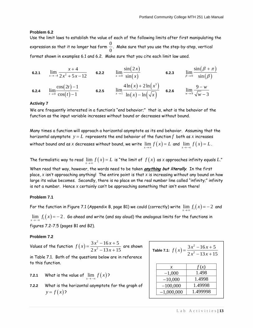
figures 7.2-7.5 (pages B1 and B2). Problem 7.2
Values of the function 2
2
3 16 52 13 15
x xf x
x x
are shown
in Table 7.1. Both of the questions below are in reference to this function. 7.2.1 What is the value of lim
xf x
?
7.2.2 What is the horizontal asymptote for the graph of y f x ?
Table 7.1: 2
2
3 16 52 13 15
x xf x
x x
x f (x)
1,000 1.498 10,000 1.4998 100,000 1.49998 1,000,000 1.499998

Portland Community College MTH 251 Lab Manual
14 | L a b A c t i v i t i e s
Problem 7.3
Jorge and Vanessa were in a heated discussion about horizontal asymptotes. Jorge said that functions never cross horizontal asymptotes. Vanessa said Jorge was nuts. Vanessa whipped out her trusty calculator and generated the values in Table 7.2 to prove her point. 7.3.1 What is the value of lim
tg t
?
7.3.2 What is the horizontal asymptote for the graph of y g t ?
7.3.3 Just how many times does the curve y g t cross
its horizontal asymptote?
Activity 8 When using limit laws to establish limit values as x or x , limit laws A1-A6 and R2 are still in play (when applied in a valid manner), but limit law R1 cannot be applied. (The reason limit law R1 cannot be applied is discussed in detail in problem 11.4) There is a new replacement law that can only be applied when x or x ; this is replacement law R3. Replacement law R3 essentially says that if the value of a function is increasing without any bound on large it becomes or if the function is decreasing without any bound on how large its absolute value becomes, then the value of a constant divided by that function must be approaching zero. An analogy can be found in extremely poor party planning. Let’s say that you plan to have a pizza party and you buy five pizzas. Suppose that as the hour of the party approaches more and more guests come in the door … in fact the guests never stop coming! Clearly as the number of guests continues to rise the amount of pizza each guest will receive quickly approaches zero (assuming the pizzas are equally divided among the guests). Problem 8.1
Consider the function 12f x
x . Complete Table
8.1 without the use of your calculator. What limit value and limit law are being illustrated in the table?
Table 7.2: sin1
tg t
t
t g (t)
103 1.0008 104 .99997 105 1.0000004 106 .9999997 107 1.00000004 108 1.000000009 109 1.0000000005 1010 .99999999995
Table 8.1: 12f x
x
x f (x)
1,000
10,000
100,000
1,000,000

Portland Community College MTH 251 Lab Manual
L a b A c t i v i t i e s | 15
Activity 9
Many limits have the form
which we take to mean that the expressions in both the numerator
and denominator are increasing or decreasing without bound. When confronted with a limit of type
limx
f x
g x or
limx
f x
g x that has the form
, we can frequently resolve the limit if we first
divide the dominant factor of the dominant term of the denominator from both the numerator and the denominator. When we do this, we need to completely simplify each of the resultant fractions and make sure that the resultant limit exists before we start to apply limit laws. We then apply the algebraic limit laws until all of the resultant limits can be replaced using limit laws R2 and R3. This process is illustrated in example 9.1. Example 9.1
2 2 2
2 22
2
2
2
13 5 3 5lim lim 13 5 3 5
53lim
3 5
5lim 3Limit Law A5
3lim 5
5lim 3 limLimit Laws A1 and A23lim lim 5
3 0 Limit Laws R2 and R30 5
35
t t
t
t
t
t t
t t
t t t t tt t
t
t
t
t
t
t
t
Problem 9.1 Use the limit laws to establish the value of each limit after dividing the dominant term-factor in the denominator from both the numerator and denominator. Remember to simplify each resultant expression before you begin to apply the limit laws.
9.1.1 2
2 3
4lim4t
t
t t 9.1.2
2
2
6 10lim2
t t
tt
e e
e
9.1.3
4 5lim5 9y
y
y
The “form” of the limit is now 3 00 5
, so we can
begin to apply the limit laws because the limits will all exist.

Portland Community College MTH 251 Lab Manual
16 | L a b A c t i v i t i e s
Activity 10 Many limit values do not exist. Sometimes the non-existence is caused by the function value either increasing without bound or decreasing without bound. In these special cases we use the symbols and to communicate the non-existence of the limits. Figures 10.1-10.3 can be used to illustrate some ways in which we communicate the non-existence of these type of limits. In Figure 10.1 we could (correctly) write
2limx
k x
, 2
limx
k x
, and 2
limx
k x
.
In Figure 10.2 we could (correctly) write
4limt
w t
, 4
limt
w t
, and 4
limt
w t
.
In Figure 10.3 we could (correctly) write
3lim
xT x
and
3lim
xT x
. There is no
shorthand way of communicating the non-existence of the two sided limit 3
limx
T x
.
Problem 10.1 Draw onto Figure 10.4 a single function, f, that satisfies each of the following limit statements. Make sure that you draw the necessary asymptotes and that you label each asymptote with its equation.
3
limx
f x
3
limx
f x
lim 0x
f x
lim 2x
f x
Figure 10.4: f
2x Figure 10.1: k 4t Figure 10.2: w 3x Figure 10.3: T

Portland Community College MTH 251 Lab Manual
L a b A c t i v i t i e s | 17
Activity 11
Whenever lim 0x a
f x
but lim 0x a
g x
, then
limx a
f x
g x does not exist because from either
side of a the value of
f x
g x either increases without bound or decreasing without bound. In
these situations the line x a is a vertical asymptote for the graph of
f xy
g x .
For example, the line 2x is a vertical asymptote for the function 52x
h xx
. We say that
2
5lim2x
x
x
has the form “not zero over zero.” (Specifically, the form of 2
5lim2x
x
x
is 70
.) Every
limit with form “not zero over zero” does not exist. However, we frequently can communicate the
non-existence of the limit using an infinity symbol. In the case of 52x
h xx
it’s pretty easy to
see that 1.99h is a positive number whereas 2.01h is a negative number. Consequently, we can
infer that 2
limx
h x
and 2
limx
h x
. Remember, these equations are communicating
that the limits do not exist as well as the reason for their non-existence. There is no short-hand way to communicate the non-existence of the two-sided limit
2limx
h x
.
Problem 11.1 Suppose that 43
tg t
t
.
11.1.1 What is the vertical asymptote on the graph of y g t .
11.1.2 Write an equality about 3
limt
g t
.
11.1.3 Write an equality about 3
limt
g t
.
11.1.4 Is it possible to write an equality about 3
limt
g t
? If so, write it.
11.1.5 Which of the following limits exist? 3
limt
g t
, 3
limt
g t
, and 3
limt
g t
Problem 11.2 Suppose that
2
2
7 32x
z xx
.
11.2.1 What is the vertical asymptote on the graph of y z x .
11.2.2 Is it possible to write an equality about 2
limx
z x
? If so, write it.
11.2.3 What is the horizontal asymptote on the graph of y z x .
11.2.4 Which of the following limits exist? 2
limx
z x
, limx
z x
, and limx
z x

Portland Community College MTH 251 Lab Manual
18 | L a b A c t i v i t i e s
Problem 11.3
Consider the function 78
xf x
x
. Complete Table 11.1 without the use of your calculator.
Use this as an opportunity to discuss why limits of form “not zero over zero” are “infinite limits.” What limit equation is being illustrated in the table? Problem 11.4 Hear me, and hear me loud … does not exist. This, in part, is why we cannot apply Limit Law R1 to an expression like lim
xx
. When we write, say,
7lim 7x
x
, we are replacing the limit
expression with its value – that’s what the replacement laws are all about ! When we write limx
x
, we are not replacing the limit expression with a value! We are explicitly saying that the
limit has no value (i.e. does not exist) as well as saying the reason the limit does not exist. The limit laws (R1-R3 and A1-A6) can only be applied when all of the limits in the equation exist. With this in mind, discuss and decide whether each of the following equations are true or false.
0
00
limlim
lim
xx
x
x xxx
ee
e e
T or F
limlim
lim
xx
x
x xxx
ee
e e
T or F
1
11
limlim
ln lim ln
xx
x
xx
ee
x x
T or F
1
11
lim lnlnlim
limx
x xxx
xx
e e
T or F
0 0
lim 2ln 2 lim lnx x
x x
T or F
lim sinsinlim
sin lim sin
T or F
lim ln lim lim lnx x
x x xe x e x
T or F
1lim1/lim xx x
xe e
T or F
Table 11.1: 78
xf x
x
x 7x 8x f (x)
8.1 15.1 .1
8.01 15.01 .01
8.001 15.001 .001
8.0001 15.0001 .0001

Portland Community College MTH 251 Lab Manual
L a b A c t i v i t i e s | 19
Problem 11.5
Mindy tried to evaluate 26
4 24lim12 36x
x
x x
using the limit laws. Things went horribly wrong for
Mindy (her work is shown below). Identify what is wrong in Mindy’s work and discuss what a more reasonable approach might have been.
226 6
6
6
6
6
6 6
4 64 24lim lim12 36 6
4lim6
lim 4Limit Law A5
lim 6
lim 4Limit Law A2
lim lim 6
4 Limit Laws R1 and R26 640
x x
x
x
x
x
x x
xx
x x x
x
x
x
Activity 12 Many statements we make about functions are only true over intervals where the function is continuous. When we say a function is continuous over an interval, we basically mean that there are no breaks in the function over that interval; that is, there are no vertical asymptotes, holes, jumps, or gaps along that interval. To make this definition more precise, we begin by defining what we mean we say that a function is continuous at the number a.
This “solution” is not correct! Do not emulate Mindy’s work!!
Definition 12.1
The function f is continuous at the number a if and only if limx a
f x f a
.
There are three ways that the defining property can fail to be satisfied at a given value of a . To facilitate exploration of these three manner of failure, we can break the defining property into a spectrum of three properties.
i. f a must be defined ii. limx a
f x
must exist iii. limx a
f x
must equal f a
Please note that if either property i or property ii fails to be satisfied at a given value of a , then property iii also fails to be satisfied at a .

Portland Community College MTH 251 Lab Manual
20 | L a b A c t i v i t i e s
Problem 12.1 State the values of t at which the function shown in Figure 12.1 is discontinuous. For each instance of discontinuity, state (by number) all of the sub-properties in Definition 12.1 that fail to be satisfied. Activity 13 When a function has a discontinuity at a , the function is sometimes continuous from only the right or only the left at a . (Please note that when we say “the function is continuous at a ” we mean that the function is continuous from both the right and left at a .) Some discontinuities are classified as removable discontinuities. Specifically, discontinuities that are holes or skips (holes with a secondary point) are called removable.
5t Figure 12.1: h
Definition 13.1 The function f is continuous from the left at a if and only if lim
x af x f a
and f is
continuous from the right at a if and only if limx a
f x f a
.
Definition 13.2 We say that f has a removable discontinuity at a if f is discontinuous at a but
limx a
f x
exists.

Portland Community College MTH 251 Lab Manual
L a b A c t i v i t i e s | 21
Problem 13.1 Referring to the function h shown in Figure 13.1, state the values of t where the function is continuous from the right but not the left. Then state the values of t where the function is continuous from the left but not the right. Problem 13.2 Referring again to the function h shown in Figure 13.1, state the values of t where the function has removable discontinuities. Activity 14 Now that we have a definition for continuity at a number, we can go ahead and define what we mean when we say a function is continuous over an interval. Problem 14.1 Write a definition for continuity over the half-open interval ,a b . Problem 14.2 Referring to the function in Figure 14.1, decide whether each of the following statements are true or false. 14.2.1 h is continuous on 4, 1
14.2.2 h is continuous on 4, 1
14.2.3 h is continuous on 4, 1
14.2.4 h is continuous on 1,2
14.2.5 h is continuous on 1,2
14.2.6 h is continuous on , 4
14.2.7 h is continuous on , 4
5t Figure 13.1: h
Definition 14.1
The function f is continuous over an open interval if and only if it is continuous at each and every number on that interval.
The function is continuous over the closed interval ,a b if and only if it is continuous
on ,a b , continuous from the right at a, and continuous from the left at b.
Similar definitions apply to half-open intervals.
5t Figure 14.1: h

Portland Community College MTH 251 Lab Manual
22 | L a b A c t i v i t i e s
Problem 14.3 Several functions are described below. Your task is to draw each function on its provided axis system. Do not introduce any unnecessary discontinuities or intercepts that are not directly implied by the stated properties. Make sure that you draw all implied asymptotes and label them with their equations. 14.3.1 Draw onto Figure 14.2 a function that satisfies all of the
following properties.
4
lim 2x
f x
4
lim 5x
f x
0 4f and 4 5f
lim lim 4x x
f x f x
14.3.2 Draw onto Figure 14.3 a function that satisfies all of the following properties.
2lim
xg x
limx
g x
0 4g , 3 2g , and 6 0g
g is continuous and has constant slope on 0, .
14.3.3 Draw onto Figure 14.4 a function that satisfies all of the
following properties.
The only discontinuities on m occur at 4 and 3 m has no x-intercepts 6 5m
4
lim 2x
m x
3
limx
m x
limx
m x
m has a constant slope of 2 over , 4
m is continuous over 4,3
Figure 14.2: f
Figure 14.3: g
Figure 14.4: m

Portland Community College MTH 251 Lab Manual
L a b A c t i v i t i e s | 23
Activity 15 Discontinuities are a little more challenging to identify when working with formulas than when working with graphs. One reason for the added difficulty is that when working with a function formula you have to dig into your memory bank and retrieve fundamental properties about certain types of functions.
Problem 15.1 15.1.1 What would cause a discontinuity on a rational function (a polynomial divided by another
polynomial)? 15.1.2 What is always true about the argument of the function, u, over intervals where the
function lny u is continuous? 15.1.3 Name three values of where the function tany is discontinuous.
15.1.4 What is the domain of the function 4k t t ?
15.1.5 What is the domain of the function 3 4g t t ?
Activity 16 Piece-wise defined functions are functions where the formula used depends upon the value of the input. When looking for discontinuities on piece-wise defined functions, you need to investigate the behavior at values where the formula changes as well as values where the issues discussed in Activity 15 might pop up. Problem 16.1 This question is all about the function f shown to the right. Answer question 16.1.1 at each of the values 1, 3, 4, 5, 7, and 8. At the values where the answer to question 16.1.1 is yes, go ahead and answer questions 16.1.2-16.1.4; skip questions 16.1.2-16.1.4 at the values where the answer to question 16.1.1 is no. 16.1.1 Is f discontinuous at the given value? 16.1.2 Is f continuous only from the left at the given value? 16.1.3 Is f continuous only from the right at the given value? 16.1.4 Is the discontinuity removable?
4 if 15
3 if 1 43
2 1 if 4 715 if 7
8
xx
xx
xf x
x x
xx

Portland Community College MTH 251 Lab Manual
24 | L a b A c t i v i t i e s
Problem 16.2 Consider the function g shown to the right. The letter C represents the same real number in all three of the piece-wise formulas. 16.2.1 Find the value for C that makes the function continuous
on ,10 . Make sure that your reasoning is clear.
16.2.2 Is it possible to find a value for C that makes the function continuous over , ? Explain.
Problem 16.3 Consider the function f shown to the right. State the values of x where each of the following occur. If a stated property doesn’t occur, make sure that you state that (as opposed to simply not responding to the question). No explanation necessary. 16.3.1 At what values of x is f discontinuous?
16.3.2 At what values of x is f continuous from the left but not the right?
16.3.3 At what values of x is f continuous from the right but not the left?
16.3.4 At what values of x does f have removable discontinuities?
if 1017
3 if 10
2 4 if 10
Cx
x
g x C x x
C x
5 if 510
5 if 5 75 30
2 if 712
xx
f x xx
xx
x

Portland Community College MTH 251 Lab Manual
L a b A c t i v i t i e s | 25
Introduction to the First Derivative Activity 17 Most of the focus in the Rates of Change lab was on average rates of change. While the idea of rates of change at one specific instant was alluded to, we couldn’t explore that idea formally because we hadn’t yet talked about limits. Now that we have covered average rates of change and limits we can put those two ideas together to discuss rates of change at specific instances in time. Suppose that an object is tossed into the air in such a way that the elevation of the object (measured in ft) is given by the function 240 40 16s t t t where t is the amount of time that
has passed since the object was tossed (measured in s). Let’s determine the velocity of the object 2 seconds into this flight.
Recall that the difference quotient 2 2s h s
h
gives us the average velocity for the object
between the times 2t and 2t h . So long as h is positive, we can think of h as the length of the time interval. To infer the velocity exactly 2 seconds into the flight we need the time interval as close to 0 as possible; this is done using the appropriate limit in example 17.1.
Example 17.1
0
2 2
0
2
0
2
0
0
0
2 22 lim
40 40 2 16 2 40 40 2 16 2lim
40 80 40 64 64 16 56lim
24 16lim
24 16lim
lim 24 16
24 16 024
h
h
h
h
h
h
s h sv
h
h h
h
h h h
h
h h
hh h
hh
From this we can infer that the velocity of the object 2 seconds into its flight is 24 ft/s. From that we know that the object is falling at a speed of 24 ft/s.

Portland Community College MTH 251 Lab Manual
26 | L a b A c t i v i t i e s
Problem 17.1 Suppose that an object is tossed into the air so that its elevation (measured in m) is given by the function 2300 10 4.9p t t t where t is the amount of time that has passed since the object
was tossed (measured in s).
17.1.1 Evaluate
0
4 4limh
p h p
h
showing each step in the simplification process (as
illustrated in example 17.1).
17.1.2 What is the unit for the value calculated in problem 17.1.1 and what does the value (including unit) tell you about the motion of the object?
17.1.3 Copy Table 17.1 onto your paper and compute and
record the missing values. Do these values support your answer to problem 17.1.2?
Activity 18 In previous activities we saw that if p is a position function, then the difference quotient for p can
be used to calculate average velocities and the expression 0 0
0limh
p t h p t
h
calculates the
instantaneous velocity at time 0t . Graphically, the difference quotient of a function f can be used to calculate the slope of secant lines to f. What happens when we take the run of the secant line to zero? Basically, we are connecting two points on the line that are really, really, (really), close to one another. As mentioned above, sending h to zero turns an average velocity into an instantaneous velocity. Graphically, sending h to zero turns a secant line into a tangent line. The tangent line to the function f x x at 4 is shown in Figure 18.1. A calculation of the slope
of this line is shown in Example 18.1.
Table 17.1: Average Velocities
1t 1
1
44
p t p
t
3.9 3.99 3.999 4.001 4.01 4.1

Portland Community College MTH 251 Lab Manual
L a b A c t i v i t i e s | 27
tan 0
0
0
0
0
0
4 4lim
4 4lim
4 2 4 2lim
4 2
4 4lim4 2
lim4 2
1lim4 2
14 0 2
14
h
h
h
h
h
h
f h fm
h
h
h
h h
h h
h
h h
h
h h
h
You should verify that the slope of the tangent line shown in Figure 18.1 is indeed 14
. You should
also verify that the equation of the tangent line is 1 14
y x .
Problem 18.1 Consider the function 5 4g x x . 18.1.1 Find the slope of the tangent line shown in Figure 18.2
using
tan 0
3 3limh
g h gm
h
. Show work
consistent with that illustrated in example 18.1.
18.1.2 Use the line in Figure 18.2 to verify your answer to problem 18.1.1.
18.1.3 State the equation of the tangent line to g at 3.
Example 18.1
Figure 18.1: f
Figure 18.2: g

Portland Community College MTH 251 Lab Manual
28 | L a b A c t i v i t i e s
Activity 19
So far we’ve seen two applications of expressions of form
0limh
f a h f a
h
. It turns out that
this expression is so important in mathematics, the sciences, economics, and many other fields that it deserves a name in and of its own right. We call the expression “the first derivative of f at a.” So far we’ve always fixed the value of a before making the calculation. There’s no reason why we couldn’t use a variable for a, make the calculation, and then replace the variable with specific values; in fact, it seems like this might be a better plan all around. This leads us to a definition of the first derivative function. As we’ve already seen, f a gives us the slope of the tangent line to f at a.
We’ve also seen that if s is a position function, then s a gives us the instantaneous velocity at a.
It’s not too much of a stretch to infer that the velocity function for s would be v t s t Problem 19.1
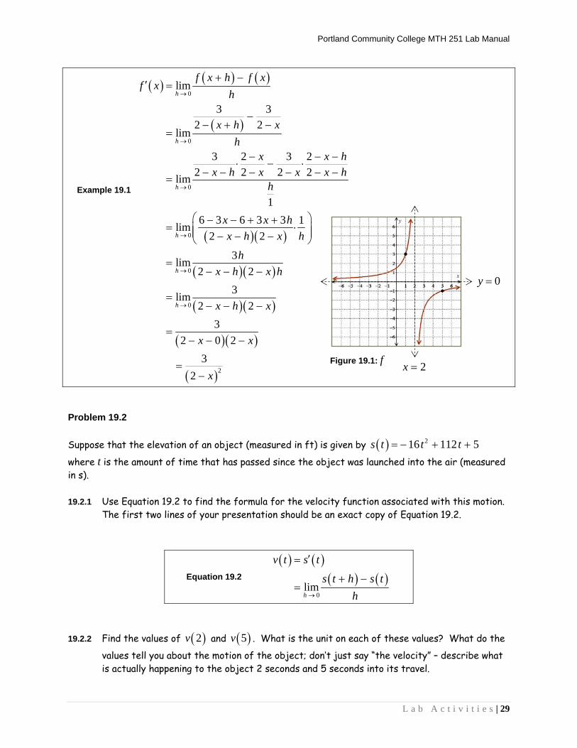
A graph of the function 32
f xx
is shown in Figure 19.1 and the formula for f x is derived
in Example 19.1.
19.1.1 Use the formula 2
32
f xx
to calculate 1f and 5f .
19.1.2 Draw onto Figure 19.1 a line through the point 1,3 with a slope of 1f . Also draw a line
though the point 5, 1 with a slope of 5f . What are the names for the two lines you
just drew? What are their equations? 19.1.3 Showing work consistent with that shown in example 19.1, find the formula for g x where
52 1
g xx
.
Definition 19.1 – The First Derivative Function
If f is a function of x, then we define the first derivative function, f , as:
0
limh
f x h f xf x
h
.
The symbols f x are read aloud as “f prime of x” or “f prime at x.”
Portland Community College MTH 251 Lab Manual
L a b A c t i v i t i e s | 29
0
0
0
0
0
0
2
lim
3 32 2
lim
3 2 3 22 2 2 2lim
16 3 6 3 3 1lim
2 2
3lim2 2
3lim2 2
32 0 2
32
h
h
h
h
h
h
f x h f xf x
h
x h x
hx x h
x h x x x hh
x x h
x h x h
h
x h x h
x h x
x x
x
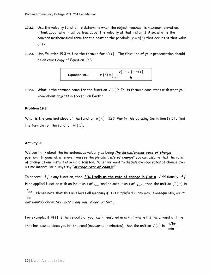
Problem 19.2 Suppose that the elevation of an object (measured in ft) is given by 216 112 5s t t t
where t is the amount of time that has passed since the object was launched into the air (measured in s). 19.2.1 Use Equation 19.2 to find the formula for the velocity function associated with this motion.
The first two lines of your presentation should be an exact copy of Equation 19.2.
Equation 19.2
0
limh
v t s t
s t h s t
h
19.2.2 Find the values of 2v and 5v . What is the unit on each of these values? What do the
values tell you about the motion of the object; don’t just say “the velocity” – describe what is actually happening to the object 2 seconds and 5 seconds into its travel.
Example 19.1
Figure 19.1: f
0y
2x
Portland Community College MTH 251 Lab Manual
30 | L a b A c t i v i t i e s
19.2.3 Use the velocity function to determine when the object reaches its maximum elevation. (Think about what must be true about the velocity at that instant.) Also, what is the common mathematical term for the point on the parabola y s t that occurs at that value
of t? 19.2.4 Use Equation 19.3 to find the formula for v t . The first line of your presentation should
be an exact copy of Equation 19.3.
Equation 19.3 0
limh
v t h v tv t
h
19.2.5 What is the common name for the function v t ? Is its formula consistent with what you
know about objects in freefall on Earth? Problem 19.3 What is the constant slope of the function 12w x ? Verify this by using Definition 19.1 to find
the formula for the function w x . Activity 20 We can think about the instantaneous velocity as being the instantaneous rate of change in position. In general, whenever you see the phrase “rate of change” you can assume that the rate of change at one instant is being discussed. When we want to discuss average rates of change over a time interval we always say “average rate of change.” In general, if f is any function, then f´(a) tells us the rate of change in f at a. Additionally, if f
is an applied function with an input unit of uniti and an output unit of unitf , then the unit on f a is
unit
unit
f
i. Please note that this unit loses all meaning if it is simplified in any way. Consequently, we do
not simplify derivative units in any way, shape, or form. For example, if v t is the velocity of your car (measured in mi/hr) where t is the amount of time
that has passed since you hit the road (measured in minutes), then the unit on v t is mi/hrmin
.
Portland Community College MTH 251 Lab Manual
L a b A c t i v i t i e s | 31
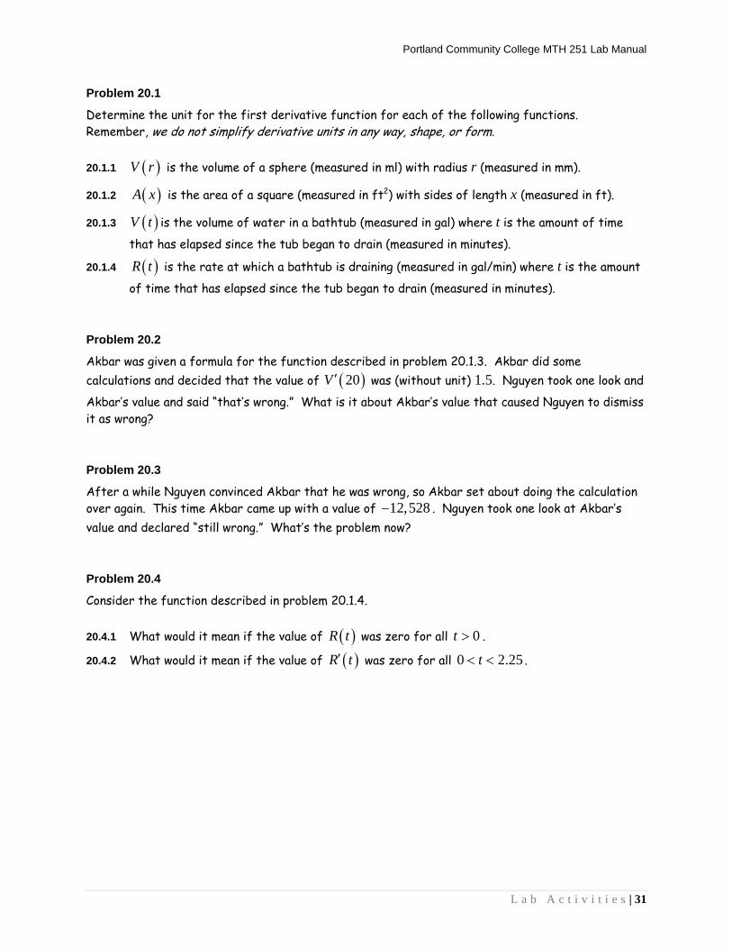
Problem 20.1
Determine the unit for the first derivative function for each of the following functions. Remember, we do not simplify derivative units in any way, shape, or form. 20.1.1 V r is the volume of a sphere (measured in ml) with radius r (measured in mm).
20.1.2 A x is the area of a square (measured in ft2) with sides of length x (measured in ft).
20.1.3 V t is the volume of water in a bathtub (measured in gal) where t is the amount of time
that has elapsed since the tub began to drain (measured in minutes).
20.1.4 R t is the rate at which a bathtub is draining (measured in gal/min) where t is the amount
of time that has elapsed since the tub began to drain (measured in minutes). Problem 20.2
Akbar was given a formula for the function described in problem 20.1.3. Akbar did some calculations and decided that the value of 20V was (without unit) 1.5. Nguyen took one look and
Akbar’s value and said “that’s wrong.” What is it about Akbar’s value that caused Nguyen to dismiss it as wrong? Problem 20.3
After a while Nguyen convinced Akbar that he was wrong, so Akbar set about doing the calculation over again. This time Akbar came up with a value of 12,528 . Nguyen took one look at Akbar’s value and declared “still wrong.” What’s the problem now? Problem 20.4
Consider the function described in problem 20.1.4. 20.4.1 What would it mean if the value of R t was zero for all 0t .
20.4.2 What would it mean if the value of R t was zero for all 0 2.25t .

Portland Community College MTH 251 Lab Manual
32 | L a b A c t i v i t i e s

Portland Community College MTH 251 Lab Manual
L a b A c t i v i t i e s | 33
Functions, Derivatives, and Antiderivatives Activity 21 Functions, derivatives, and antiderivatives have many entangled properties. For example, over intervals where the first derivative of a function is always positive, we know that the function itself is always increasing. (Do you understand why?) Many of these relationships can be expressed graphically. Consequently, it is imperative that you fully understand the meaning of some commonly used graphical expressions. These expressions are loosely defined in Table 21.1.
Table 21.1: Some Common Graphical Phrases The function is positive
This means that the vertical-coordinate of the point on the function is positive. As such, a function is positive whenever it lies above the horizontal axis.
The function is negative
This means that the vertical-coordinate of the point on the function is negative. As such, a function is negative whenever it lies below the horizontal axis.
The function is increasing
This means that the vertical-coordinate of the function consistently increases as you move along the curve from left to right. Linear functions with positive slope are always increasing.
The function is decreasing
This means that the vertical-coordinate of the function consistently decreases as you move along the curve from left to right. Linear functions with negative slope are always decreasing.
The function is concave up
A function is concave up at a if the tangent line to the function at a lies below the curve. An upward opening parabola is everywhere concave up.
The function is concave down
A function is concave down at a if the tangent line to the function at a lies above the curve. A downward opening parabola is everywhere concave down.
Problem 21.1 Answer each of the following questions in reference to the function shown in Figure 21.1. Each answer is an interval (or intervals) along the x-axis. Use interval notation when expressing your answers. Make each interval as wide as possible; that is, do not break an interval into pieces if the interval does not need to be broken up. Assume that the slope of the function is constant on , 5 , 3,4 , and 4, .
21.1.1 Over what intervals is the function positive? 21.1.2 Over what intervals is the function negative? 21.1.3 Over what intervals is the function increasing? 21.1.4 Over what intervals is the function decreasing? 21.1.5 Over what intervals is the function concave up? 21.1.6 Over what intervals is the function concave down? 21.1.7 Over what intervals is the function linear? 21.1.8 Over what intervals is the function constant?
Figure 21.1: f

Portland Community College MTH 251 Lab Manual
34 | L a b A c t i v i t i e s
Activity 22 Much information about a function’s first derivative can be gleaned simply by looking at a graph of the function. In fact, a person with good visual skills can “see” the graph of the derivative while looking at the graph of the function. This activity focuses on helping you develop that skill. Problem 22.1 A parabolic function is shown in Figure 22.1. Each question in this problem is in reference to that function.
22.1.1 Several values of the function g are given in Table 22.1. For each given value draw a nice long line segment at the corresponding point on g whose slope is equal to the value of g . If we think of these line segments as actual lines, what do we call the lines?
22.1.2 What is the value of g at 1? How do you know? Go ahead and enter that value into Table 22.1.
22.1.3 The function g is symmetric across the line 1x ; that is, if we move equal distance to the left and right from this line the corresponding y-coordinates on g are always equal. Notice that the slopes of the tangent lines are “equal but opposite” at points that are equally removed from the axis of symmetry; this is reflected in the values of 1g and 3g .
Use the idea of “equal but opposite slope equidistance from the axis of symmetry” to complete Table 22.1.
22.1.4 Plot the points from Table 22.1 onto Figure 22.2 and connect the dots. Determine the formula for the resultant linear function.
22.1.5 The formula for g is 2.5 5.5g x x x . Use Definition 19.1 to determine the formula
for g x .
22.1.6 The line you drew onto Figure 22.2 is not a tangent line to g. Just what exactly is this line?
Figure 22.1: g Figure 22.2: g
Table 22.1: y g x
x y
5 6
3
1 2
1
3 2
5 4
7

Portland Community College MTH 251 Lab Manual
L a b A c t i v i t i e s | 35
Problem 22.2 A function f is shown in Figure 22.3 and the corresponding first derivative function f is shown in Figure 22.4. Answer each of the following questions referencing these two functions. 22.2.1 Draw the tangent line to f at the three points indicated in Figure 22.3 after first using the
graph of f to determine the exact slope of the respective tangent lines.
22.2.2 Write a sentence relating the slope of the tangent line to f with the corresponding y-coordinate on f .
22.2.3 Copy each of the following phrases onto your paper and supply the words or phrases that correctly complete each sentence.
Over the interval where f is always negative f is always . Over the intervals where f is always positive f is always . Over the interval where f is always increasing f is always . Over the interval where f is always decreasing f is always .
Problem 22.3 In each of figures 22.5 and 22.6 a function (the thin curve) is given; both of these functions are symmetric about the y-axis. The first derivative of each function (the thick curves) have been drawn over the interval 0,7 . Use the given portion of the first derivative together with the
symmetry of the function to help you draw each first derivative over the interval 7,0 .
Figure 22.3: f Figure 22.4: f
Figure 22.5: g and g Figure 22.6: k and k
0.5y
0x

Portland Community College MTH 251 Lab Manual
36 | L a b A c t i v i t i e s
Problem 22.4
A graph of the function 1
yx
is shown in Figure 22.7; call this function f.
22.4.1 Except at 0, there is something that is always true about the value of f ; what is the common trait?
22.4.2 Use Definition 19.1 to find the formula for f x .
22.4.3 Does the formula for f x support your answer to problem 22.4.1?
22.4.4 Use the formula for f x to determine the horizontal and vertical asymptotes for the
graph of y f x .
22.4.5 Keeping it simple, draw onto Figure 22.8 a curve with the asymptotes found in problem 22.4.4 and the property determined in problem 22.4.1. Does the curve you drew have the properties you would expect to see in the first derivative of f ? For example, f is concave down over ,0 and concave up over 0, ; what are the corresponding differences in
the behavior of f over those two intervals? Problem 22.5 A graph of the function g is shown in Figure 22.9. The absolute minimum value ever obtained by g is 3 . With that in mind, draw g onto Figure 22.10. Make sure that you draw and label any and all necessary asymptotes. Make sure that your graph of g adequately reflects the symmetry in the graph of g .
Figure 22.8: f Figure 22.7: f 0x
0y
1y
5y
Figure 22.9: g Figure 22.10: g

Portland Community College MTH 251 Lab Manual
L a b A c t i v i t i e s | 37
Problem 22.6 A function, w, is shown in Figure 22.11. A larger version of Figure 22.11 is available in Appendix B (page B3). Answer each of the following questions in reference to this function. 22.6.1 An inflection point is a point where the function is continuous and the concavity of the
function changes. The inflection points on w occur at 2, 3.25, and 6. With that in mind, over each interval stated in Table 22.3 exactly two of the words in Table 22.2 apply to w . Complete Table 22.2 with the appropriate pairs of words.
22.6.2 In Table 22.4, three possible values are given for w at several values of x. In each case,
one of the values is correct. Use tangent lines to w to determine each of the correct values. (This is where you probably want to use the graph on page B3.)
22.6.3 The value of w is the same at 2, 4, and 7. What is this common value? 22.6.4 Put it all together and draw w onto Figure 22.12.
Table 22.3: Properties of w Interval Properties
, 2
2,3.25
3.25,4
4,6
6,7
7,
Table 22.2: Properties positive negative
increasing decreasing
Figure 22.11: w
Table 22.4: Choose the correct values for w x Proposed values
0 23 or 8
3 or 283
1 12 or 3
2 or 52
3 13 or 1 or 3
5 12 or 1 or 3
2
6 43 or 8
3 or 4
8 1 or 6 or 12
Figure 22.12: w

Portland Community College MTH 251 Lab Manual
38 | L a b A c t i v i t i e s
Activity 23 A function is said to be nondifferentiable at any value its first derivative is undefined. There are three graphical behaviors that lead to non-differentiability.
f is nondifferentiable at a if f is discontinuous at a. f is nondifferentiable at a if the slope of f is different from the left and right at a. f is nondifferentiable at a if f has a vertical tangent line at a.
Problem 23.1 Consider the function k shown in Figure 23.1.
23.1.1 There are four values where k is nondifferentiable; what are these values? 23.1.2 Draw k onto Figure 23.2.
Problem 23.2 Consider the function g shown in Figure 23.3.
23.2.1 g has been drawn onto Figure 23.4 over the interval 5, 2.5 . Use the piece-wise
symmetry and periodic behavior of g to help you draw the remainder of g over 7,7
23.2.2 What six syllable word applies to g at 5, 0, and 5? 23.2.3 What five syllable and six syllable words apply to g at 5, 0, and 5?
Figure 23.1: k Figure 23.2: k
Figure 23.3: g Figure 23.4: g

Portland Community College MTH 251 Lab Manual
L a b A c t i v i t i e s | 39
Activity 24 Seeing as the first derivative of f is a function in its own right, f must have its own first derivative. The first derivative of f is the second derivative of f and is symbolized as f (f double-prime). Likewise, f (f triple-prime) is the first derivative of f , the second derivative of f , and the third derivative of f.
All of the graphical relationships you’ve established between f and f work their way down the derivative chain; this is illustrated in tables 24.1, 24.2, and 24.3. Problem 24.1 Extrapolating from tables 24.1 and 24.2, what must be true about f over intervals where f is, respectively, positive, negative, and constantly zero? Problem 24.2 A function, g, and its first three derivatives are shown in figures 24.1-24.4, although not in that order. Determine which curve is which function ( g , g , g , and g ).
Table 24.1: f and f
When f is … f is … Positive Increasing Negative Decreasing Constantly Zero Constant Increasing Concave Up Decreasing Concave Down Constant Linear
Table 24.2: f and f
When f is … f is … Positive Increasing Negative Decreasing Constantly Zero Constant Increasing Concave Up Decreasing Concave Down Constant Linear
Table 24.3: f and f When f is … f is … Positive Increasing Negative Decreasing Constantly Zero Constant Increasing Concave Up Decreasing Concave Down Constant Linear
Figure 24.1
Figure 24.2 Figure 24.3 Figure 24.4

Portland Community College MTH 251 Lab Manual
40 | L a b A c t i v i t i e s
Problem 24.3 Three containers are shown in figures 24.5-24.7. Each of the following questions are in reference to these containers. 24.3.1 Suppose that water is being poured into each of the containers at a constant rate. Let 5h ,
6h , and 7h be the heights (measured in cm) of the liquid in containers 24.5-24.7, respectively, t seconds after the water began to fill the containers. What would you expect
the sign to be on the second derivative functions 5h , 6h , 7h while the containers are
being filled? (Hint: Think about the shape of the curves 5y h t , 6y h t , and
7y h t .)
24.3.2 Suppose that water is being drained from each of the containers at a constant rate. Let 5h ,
6h , and 7h be the heights (measured in cm) of the liquid remaining in the containers t seconds after the water began to drain. What would you expect the sign to be on the
second derivative functions 5h , 6h , 7h while the containers are being drained? Problem 24.4 During the recession of 2008-2009, the total number of employed Americans decreased every month. One month a talking head on the television made the observation that “at least the second derivative was positive this month.” Why was it a good thing that the second derivative was positive? Problem 24.5 During the early 1980s the problem was inflation. Every month the average price for a gallon of milk was higher than the month before. Was it a good thing when the second derivative of this function was positive? Explain.
Figure 24.5 Figure 24.7 Figure 24.6

Portland Community College MTH 251 Lab Manual
L a b A c t i v i t i e s | 41
Activity 25 The derivative continuum can be expressed backwards as well as forwards. When you move from function to function in the reverse direction the resultant functions are called antiderivatives and the process is called antidifferentiation. These relationships are shown in figures 25.1 and 25.2.
differentiate differentiate differentiate differentiatef f f f
Figure 25.1: Differentiating
antidifferentiate antidifferentiate antidifferentiate antidifferentiate antidifferentiatef f f f F
Figure 25.2: Antidifferentiating There are (at least) two important differences between the differentiation chain and the antidifferentiation chain (besides their reversed order).
When you differentiate, the resultant function is unique. When you antidifferentiate, you do not get a unique function - you get a family of functions; specifically, you get a set of parallel curves.
We introduce a new function in the antidifferentiation chain. We say that F is an
antiderivative of f. This is where we stop in that direction; we do not have a variable name for an antiderivative of F.
Since F is considered an antiderivative of f, it must be the case that f is the first derivative of F. Hence we can add F to our derivative chain resulting in Figure 25.3
differentiate differentiate differentiate differentiate differentiateF f f f f
Figure 25.3: Differentiating Problem 25.1 Each of the linear functions in Figure 25.4 have the same first derivative function. 25.1.1 Draw this common first derivative function onto Figure
25.4 and label it g. 25.1.2 Each of the given lines Figure 25.4 is called what in
relation to g?
Figure 25.4

Portland Community College MTH 251 Lab Manual
42 | L a b A c t i v i t i e s
Figure 25.6 Figure 25.7 Figure 25.8
Problem 25.2 The function f is shown in Figure 25.5. Reference this function in the following questions. 25.2.1 At what values of x is f nondifferentiable? 25.2.2 At what values of x are antiderivatives of f nondifferentiable? 25.2.3 Draw onto Figure 25.6 the continuous antiderivative of f
that passes through the point 3,1 . Please note that
every antiderivative of f increases exactly one unit over the interval 3, 2 .
25.2.4 Because f is not continuous, there are other antiderivatives of f that pass through the point 3,1 .
Specifically, antiderivatives of f may or may not be continuous at 1 . Draw onto figures 25.7 and 25.8 different antiderivatives of f that pass through the point 3,1 .
Problem 25.3 The function siny x is an example of a periodic function. Specifically, the function has a
period of 2 because over any interval of length 2 the behavior of the function is exactly the
same as it was the previous interval of length 2 . A little more precisely, sin 2 sinx x
regardless of the value of x. Jasmine was thinking and told her lab assistant that derivatives and antiderivatives of periodic functions must also be periodic. Jasmine’s lab assistant told her that she was half right. Which half did Jasmine have correct? Also, draw a function that illustrates that the other half of Jasmine’s statement is not correct.
Figure 25.5: f

Portland Community College MTH 251 Lab Manual
L a b A c t i v i t i e s | 43
Problem 25.4 Consider the function g shown in Figure 25.9.
25.4.1 Let G be an antiderivative of g. Suppose that G is continuous on 6,6 , 6 3G , and
that the greatest value G ever achieves is 6. Draw G onto Figure 25.10. 25.4.2 At what values of t is G nondifferentiable? 25.4.3 At what values of t is g nondifferentiable?
Problem 25.5 Answer the following question in reference to a continuous function g whose first derivative is shown in Figure 25.11. You do not need to state how you made your determination; just state the interval(s) or values of x that satisfy the stated property. Note: The correct answer to one or more of these questions
may be “There is no way of knowing.” 25.5.1 Over these intervals, g is positive and increasing. 25.5.2 At these values of x , g is nondifferentiable. 25.5.3 Over these intervals, g is never negative. 25.5.4 At these values of x , every antiderivative of g is
nondifferentiable. 25.5.5 Over these intervals, the value of g is constant. 25.5.6 Over these intervals, g is linear. 25.5.7 Over these intervals, antiderivatives of g are linear. 25.5.8 Over these intervals, g is never negative.
Figure 25.10 G Figure 25.9 g
Figure 25.11 g

Portland Community College MTH 251 Lab Manual
44 | L a b A c t i v i t i e s
Figure 26.2 g
Figure 26.1 f
Activity 26 When given a function formula, we often find the first and second derivative formulas to determine behaviors of the given function. In a later lab we will use the first and second derivative formulas to help us graph a function given the formula for the function. One thing we do with the derivative formulas is determine where they are positive, negative, zero, and undefined. This helps us determine where the given function is increasing, decreasing, concave up, concave down, and linear. Problem 26.1 26.1.1 Draw onto Figure 26.1 a continuous function f that has a horizontal tangent line at the point
1,2 along with the properties stated in Table 26.1.
26.1.2 Given the conditions stated in problem 26.1.1, does it have to be the case that 1 0f ?
26.1.3 Is f increasing at 1 ? How do you know? 26.1.4 Can a continuous, everywhere differentiable function satisfy the properties stated in Table
26.1 and not have a slope of zero at 1 ? Draw a picture that supports your answer. Problem 26.2 26.2.1 Draw onto Figure 26.2 a continuous function g that has a vertical tangent line at the point
1,2 along with the properties stated in Table 26.2.
26.2.2 Given the conditions stated in problem 26.2.1, does it have to be the case that 1g is
undefined? 26.2.3 Is g increasing at 1 ? How do you know? 26.2.4 Can a continuous, everywhere differentiable function satisfy the properties stated in Table
26.2 and not have a vertical tangent line at 1 ? Draw a picture that supports your answer.
Table 26.1: Signs on f and f Interval f f
, 1 Positive Negative
1, Positive Positive
Table 26.2: Signs on g and g Interval g g
, 1 Positive Positive
1, Positive Negative

Portland Community College MTH 251 Lab Manual
L a b A c t i v i t i e s | 45
Figure 26.3 k
Problem 26.3 26.3.1 Draw onto Figure 26.3 a continuous function k that passes through the point 1,2 and
also satisfies the properties stated in Table 26.3. 26.3.2 At what values of x is k nondifferentiable? Problem 26.4
You should know by now that the first derivative continually increases over intervals where the second derivative is constantly positive and that the first derivative continually decreases over intervals where the second derivative is constantly negative. A person might infer from this that a function changes more and more quickly over intervals where the second derivative is constantly positive and that a function changes more and more slowly over intervals where the second derivative is constantly negative. We are going to explore that idea in this problem.
26.4.1 Suppose that V t is the volume of water in an ice cube (ml) where t is the amount of time
that has passed since noon (measure in minutes). Suppose that mlmin6 0V and that
V t has a constant value of ml
minmin
.3 over the interval 6,11 . What is the value of
11V ? When is V changing more quickly, at 12:06 pm or at 12:11 pm?
26.4.2 Referring to the function V in problem 26.4.1, what would the shape of V be over the interval 6,11 ? (Choose from options a – d.)
26.4.3 Again referring to options a-d, which functions are changing more and more rapidly from left to right and which functions are changing more and more slowly from left to right? Which functions have positive second derivatives and which functions have negative second derivatives? Do the functions with positive second derivative values both change more and more quickly from left to right?
Table 26.3: Signs on k and k Interval k k
, 1 Negative Positive
1, Positive Negative
a cb d

Portland Community College MTH 251 Lab Manual
46 | L a b A c t i v i t i e s
26.4.4 Consider the signs on both the first and second derivatives in options a-d. Is there something that the two functions that change more and more quickly have in common that is different in the functions that change more and more slowly?
Problem 26.5 Resolve each of the following disputes. 26.5.1 One day Sara and Jermaine were working on an assignment. One question asked them to
draw a function over the domain 2, with the properties that the function is always
increasing and always concave down. Sara insisted that the curve must have a vertical asymptote at 2 and Jermaine insisted that the function must have a horizontal asymptote somewhere. Were either of these students correct?.
26.5.2 The next question Sara and Jermaine encountered described the same function with the
added condition that the function is never positive. Sara and Jermaine made the same contentions about asymptotes. Is one of them now correct?
26.5.3 At another table Pedro and Yoshi were asked to draw a continuous curve that, among other
properties, was never concave up. Pedro said ”OK, so the curve is always concave down” to which Yoshi replied “Pedro, you need to open your mind to other possibilities.” Who’s right?
26.5.4 In the next problem Pedro and Yoshi were asked to draw a function that is everywhere
continuous and that is concave down at every value of x except 3. Yoshi declared “impossible” and Pedro responded “have some faith, Yosh-man.” Pedro then began to draw. Is it possible that Pedro came up with such a function?
Problem 26.6 Determine the correct answer to each of the following questions. Pictures of the situation may help you determine the correct answers. 26.6.1 Which of the following propositions is true? If a given proposition is not true, draw a graph
that illustrates its untruth.
26.6.1a If the graph of f has a vertical asymptote, then the graph of f must also have a vertical asymptote.
26.6.1b If the graph of f has a vertical asymptote, then the graph of f must also have a vertical asymptote.
26.6.2 Suppose that the function f is everywhere continuous and concave down. Suppose further
that 7 5f and 7 3f . Which of the following is true?
a. 9 11f b. 9 11f c. 9 11f
d. There is not enough information to determine the relationship between 9f and 11.

Portland Community College MTH 251 Lab Manual
L a b A c t i v i t i e s | 47
Derivative Formulas Activity 27 While the primary focus of this lab is to help you develop shortcut skills for finding derivative formulas, there are inevitable notational issues that must be addressed. It turns out that the latter issue is the one we are going to address first. If y f x , we say that the derivative of y with respect to x is equal to f x . Symbolically
we write: dyf x
dx
If z g t , we say that the the derivative of z with respect to t is equal to g t . Symbolically
we write: dzg t
dt . (Read aloud as “d-z-d-t equals g-prime of t.”)
Problem 27.1 Take the derivative of both sides of each equation with respect to the independent variable as indicated in the function notation. Write and say the derivative using Leibniz notation on the left side of the equal sign and function notation on the right side of the equal sign. Make sure that every one in your group says at least one of the derivative equations aloud using both the formal reading and informal reading of the Leibniz notation. 27.1.1 y k t 27.1.2 V f r 27.1.3 T g P
Activity 28 dy
dx is the name of a derivative in the same way that f x is the name of a derivative. We need
a different symbol that tells us to take the derivative of a given expression (in the same way that we have symbols that tell us to take a square root, sine, or logarithm of an expression).
The symbol d
dx is used to tell us to take the derivative with respect to x of something. The
symbol itself is an incomplete phrase in the same way that the symbol is an incomplete phrase; in both cases we need to indicate the object to be manipulated – what number or formula are we taking the square root of? … what number or formula are we differentiating?
While the symbol dy
dx certainly looks like a fraction, it is not a fraction. The symbol is
Leibniz notation for the first derivative of y with respect to x. The short way of reading the symbol aloud is “d-y-d-x” (don’t enunciate the dashes).

Portland Community College MTH 251 Lab Manual
48 | L a b A c t i v i t i e s
One thing you can do to help you remember the difference between the symbols dy
dx and
d
dx is to
get in the habit of always writing grouping symbols after d
dx. In this way the symbols sind
xdx
mean “the derivative with respect to x of the sine of x.” Similarly, the symbols 2dt
dt mean “the
derivative with respect to t of t-squared.” Problem 28.1
Write the Leibniz notation for each of the following expressions. 28.1.1 The derivative with respect to of cos .
28.1.2 The derivative with respect to x of dy
dx.
28.1.3 The derivative with respect to t of ln x . (Yes, we will do such things.)
28.1.4 The derivative of z with respect to x. 28.1.5 The derivative with respect to t of 8g . (Yes, we will also do such things.)
Activity 29 The first differentiation rule we are going to explore is called the power rule of differentiation.
Equation 29.1 1 for n 0n ndx n x
dx
When n is a positive integer, it is fairly easy to establish this rule using Definition 19.1. The proof of the rule gets a little more complicated when n is negative, fractional, or irrational. For purposes of this lab, we are going to just accept the rule as valid. This rule is one you just “do in your head” and then write down the result. Three examples of what you would be expected to write when differentiating power functions are shown below.
Given Function
7y x 3 7f t t 5
1z
y
What you should think or write (as necessary)
7y x 7/3f t t 5z y
What you should write
67dyx
dx
4/3
43
7373
f t t
t
6
6
5
5
dzy
dy
y

Portland Community College MTH 251 Lab Manual
L a b A c t i v i t i e s | 49
Notice that the type of notation used when naming the derivative is dictated by the manner in which the original function is expressed. For example, 7y x is telling us the relationship between
two variables; in this situation we name the derivative using the notation dy
dx. On the other hand,
function notation is being used to name the rule in 3 7f t t ; in this situation we name the
derivative using the function notation f t .
Problem 29.1
Find the first derivative formula for each of the following functions. In each case take the derivative with respect to the independent variable as implied by the expression on the right side of the equal sign. Make sure that you use the appropriate name for each derivative.
29.1.1 43f x x 29.1.2 7
1z
t 29.1.3 5 2P t 29.1.4 1
h xx
Activity 30
The next rule you are going to practice is the constant factor rule of differentiation. This is another rule you do in your head.
Equation 30.1 ford dk f x k f x k
dx dx
In the following examples and problems several derivative rules are used that are shown in Appendix C (pages C5 and C6). While working this lab you should refer to those rules; you may want to cover up the chain rule and implicit derivative columns this week! You should make a goal of having all of the basic formulas memorized within a week. Given Function 96f x x 2cosf 2lnz x
What you should write
854f x x 2sinf 2dz
dx x
Problem 30.1
Find the first derivative formula for each of the following functions. In each case take the derivative with respect to the independent variable as implied by the expression on the right side of the equal sign. Make sure that you use the appropriate name for each derivative.
30.1.1 47z t 30.1.2 7sinP x x 30.1.3 1 ln3
h t t
30.1.4 tanz x x 30.1.5 4
8P
t
30.1.6 4T t

Portland Community College MTH 251 Lab Manual
50 | L a b A c t i v i t i e s
Activity 31
When an expression is divided by the constant k, we can think of the expression as being multiplied
by the fraction 1k
. In this way, the constant factor rule of differentiation can be applied when a
formula is multiplied or divided by a constant.
Given Function
4
8x
f x 3tan
2y
ln3
yz
What you should think 41
8f x x 3 tan
2y 1 ln
3z y
What you should write 31
2f x x 23 sec
2dy
d
13
dz
dy y
Problem 31.1
Find the first derivative formula for each of the following functions. In each case take the derivative with respect to the independent variable as implied by the expression on the right side of the equal sign. Make sure that you use the appropriate name for each derivative.
31.1.1 1sin6
tz t
31.1.2 3
3r
V r
31.1.3 1 22
G m mf r
r
G, m1, and m2 are constants.
Activity 32
When taking the derivative of two or more terms, you can take the derivatives term by term and insert plus or minus signs as appropriate. Collectively we call this the sum and difference rules of differentiation.
Equation 32.1 d d df x g x f x g x
dx dx dx
In the following examples and problems we introduce linear and constant terms into the functions being differentiated.
Equation 32.2 0 fordk k
dx Equation 32.3 ford
k x k kdx
Problem 32.1
Explain why both the constant rule (Equation 32.2) and linear rule (Equation 32.3) are “obvious.”
Hint: Think about the graphs y k and y k x . What does a first derivative tell you about a graph?

Portland Community College MTH 251 Lab Manual
L a b A c t i v i t i e s | 51
A couple of examples using the sum and difference rule are shown below.
Given Function
5 6 14 86
y t tt
sin cos4
2P
What you should think or write (as necessary)
6/5 1/ 214 86
y t t t 1 1sin cos 42 2
P
What you should definitely write
1/5 3/ 2
5
3
24 1 85 1224 1 8
5 12
dyt t
dt
t
t
1 1cos sin
2 2P
Problem 32.2 Find the first derivative formula for each of the following functions. In each case take the derivative with respect to the independent variable as implied by the expression on the right side of the equal sign. Make sure that you use the appropriate name for each derivative.
32.2.1 sin 2cos 3T t t 32.2.2 4sec 3csc4
k
32.2.3 75x
r x 32.2.4 3
ln2 ln 293
xr
x
Activity 33
The next rule we are going to explore is called the product rule of differentiation. We use this rule when there are two or more variable factors in the expression we are differentiating. (Remember, we already have the constant factor rule to deal with two factors when one of the two factors is a constant.)
Equation 33.1 d d df x g x f x g x f x g x
dx dx dx
Intuitively, what is happening in this rule is that we are alternately treating one factor as a constant (the one not being differentiated) and the other factor as a variable function (the one that is being differentiated). We then add these two rates of change together. Ultimately, you want to perform this rule in your head just like all of the other rules. Your instructor, however, may initially want you to show steps; under that presumption, steps are going to be shown in each and every example of this lab when the product rule is applied. Two simple examples of the product rule are shown at the top of the next page.

Portland Community College MTH 251 Lab Manual
52 | L a b A c t i v i t i e s
Given Function
2 siny x x x costP e t
Derivative
2 2
2
sin sin
2 sin cos
d dy x x x x x
dx dx
x x x x
cos cos
cos sin
t t
t t
dP d de t e t
dt dt dt
e t e t
A decision you’ll need to make is how to handle a constant factor in a term that requires the product rule. Two options for taking the derivative of 25 lnf x x x are shown below.
Option A
2 2
2
5 ln ln
15 2 ln
10 ln 5
d df x x x x x
dx dx
x x xx
x x x
Option B
2 2
2
5 ln 5 ln
110 ln 5
10 ln 5
d df x x x x x
dx dx
x x xx
x x x
In Option B we are treating the factor of 5 as a part of the first variable factor. In doing so, the factor of 5 distributes itself. This is the preferred treatment of the author, so this is what you will see illustrated in this lab. Problem 33.1
Find the first derivative formula for each of the following functions. In each case take the derivative with respect to the independent variable as implied by the expression on the right side of the equal sign. Make sure that you use the appropriate name for each derivative.
33.1.1 2sec tanT t t t 33.1.2 2
te tk
33.1.3 34 ln 3xy x x x 33.1.4 cot cot 1f x x x
Problem 33.2
Find each of the following derivatives without first simplifying the formula; that is, go ahead and use the product rule on the expression as written. Simplify each resultant derivative formula. For each derivative, check your answer by simplifying the original expression and then taking the derivative of that simplified expression.
33.2.1 4 7dx x
dx 33.2.2 10d
x xdx
33.2.3 21dx x
dx

Portland Community College MTH 251 Lab Manual
L a b A c t i v i t i e s | 53
Activity 34 The next rule we are going to explore is called the quotient rule of differentiation. We never use this rule unless there is a variable factor in the denominator of the expression we are differentiating. (Remember, we already have the constant factor rule to deal with constant factors in the denominator.)
Equation 34.1
2 ; 0
d df x g x f x g xf xd dx dx g x
dx g x g x
Like all of the other rules, you ultimately want to perform the quotient rule in your head. Your instructor, however, may initially want you to show steps when applying the quotient rule; under that presumption, steps are going to be shown in each and every example of this lab when the quotient rule is applied. Two simple examples of the quotient rule are shown below. Given Function
34ln
xy
x
csctan
tV
t
Derivative
3 3
2
2 3
2
2 2
2
4 ln 4 ln
ln
112 ln 4
ln
12 ln 4
ln
d dx x x xdy dx dx
dx x
x x xx
x
x x x
x
2
2
2
2
2
csc tan csc tan
tan
csc cot tan csc sectan
csc 1 sec
tan
d dt t t tdV dt dt
dt t
t t t t t
t
t t
t
Problem 34.1 Find the first derivative formula for each of the following functions. In each case take the derivative with respect to the independent variable as implied by the expression on the right side of the equal sign. Make sure that you use the appropriate name for each derivative.
34.1.1 4ln xg x
x 34.1.2
53
cosy
j yy
34.1.3
sin4sec
xy
x 34.1.4
2
t
tf t
e
Problem 34.2 Find each of the following derivatives without first simplifying the formula; that is, go ahead and use the quotient rule on the expression as written. For each derivative, check your answer by simplifying the original expression and then taking the derivative of that simplified expression.
34.2.1
sinsin
td
dt t
34.2.2 6
2
d x
dx x
34.2.3 102
d
dx x

Portland Community College MTH 251 Lab Manual
54 | L a b A c t i v i t i e s
Activity 35 In problems 33.2 and 34.2 you applied the product and quotient rules to expressions where the derivative could have been found much more quickly had you simplified the expression before taking the derivative. For example, while you can find the correct derivative formula using the quotient rule when working problem 34.2.3, the derivative can be found much more quickly if you simplify the expression before applying the rules of differentiation. This is illustrated in Example 35.1.
Example 35.1
1
2
2
10 52
55
d dx
dx x dx
x
x
Part of learning to take derivatives is learning to make good choices about the methodology to employ when taking derivatives. In examples 35.2 and 35.3, the need to use the product rule or quotient rule is obviated by first simplifying the expression being differentiated.
Example 35.2
Problem
Find dy
dx if sec cosy x x .
Solution
sec cos1 cos
cos1
0
y x x
xx
dy
dx
Example 35.3 Problem
Find f t if 5 3
2
4 32
t tf t
t
.
Solution
5 3
2
5 3
2 2
3
2
4 32
4 32 2
322362
t tf t
t
t t
t t
t t
f t t

Portland Community College MTH 251 Lab Manual
L a b A c t i v i t i e s | 55
Problem 35.1 Find the derivative with respect to x for each of the following functions after first completely simplifying the formula being differentiated. In each case you should not use either the product rule or the quotient rule while finding the derivative formula.
35.1.1 12 4 2
4
4 5 3x x xy
x
35.1.2
4sincos
xg x
x
35.1.3
6
2
43
xh x
x
35.1.4 2 2sin cosz x x x 35.1.5 4 4z x x 35.1.6 2
lnln
xT x
x
Activity 36 Sometimes both the product rule and quotient rule need to be applied when finding a derivative formula. Problem 36.1
Consider the functions 2 sinx
xf x x
e and 2 sin
x
x xg x
e .
36.1.1 Discuss why f and g are in fact two representations of the same function.
36.1.2 Find f x by first applying the product rule and then applying the quotient rule (where
necessary).
36.1.3 Find g x by first applying the quotient rule and then applying the product rule (where
necessary).
36.1.4 Rigorously establish that the formulas for f x and g x are indeed the same.
Activity 37 Derivative formulas can give us much information about the behavior of a function. For example, the derivative formula for 2f x x is 2f x x . Clearly f is negative when x is negative and
f is positive when x is positive. This tells us that f is decreasing when x is negative and that f is
increasing when x is positive. This matches the behavior of the parabola 2y x .

Portland Community College MTH 251 Lab Manual
56 | L a b A c t i v i t i e s
Problem 37.1 Answer each of the following questions about applied functions. 37.1.1 The amount of time (seconds), T, required for a pendulum to complete one period is a
function of the pendulum’s length (meters), L. Specifically, 2 LT
g where g is the
acceleration constant for Earth (roughly 9.8 m/s2).
37.1.1.a Find dT
dL after first rewriting the formula for T as a constant times L .
37.1.1.b The sign on dT
dL is the same regardless of the value of L. What is this sign and
what does it tell you about the relative periods of two pendulums with different lengths?
37.1.2 The gravitational force (Newtons) between two objects of masses 1m and 2m (kg) is a
function of the distance (meters) between the objects’ centers of mass, r. Specifically,
1 22
G m mF r
r where G is the universal gravitational constant (which is approximately
11 26.7 10 n m/kg ).
37.1.2.a Leaving G, 1m , and 2m as constants, find F r after first rewriting the formula
for F as a constant times a power of r.
37.1.2.b The sign on F r is the same regardless of the value of F. What is this sign and
what does it tell you about the effect on the gravitational force between two objects when the distance between the objects is changed?
37.1.2.c Leaving G, 1m , and 2m as constants, evaluate 121.00 10F , 121.01 10F ,
121.02 10F .
37.1.2.d Calculate 12 12
12 12
1.02 10 1.00 101.02 10 1.00 10
F F
. Which of the quantities found in part c
comes closest to this value? Draw a sketch of F and discuss why this result makes sense.

Portland Community College MTH 251 Lab Manual
L a b A c t i v i t i e s | 57
The Chain Rule Activity 38 The functions sinf t t and sin 3k t t are shown in Figure
38.1. Since cosf t t , it is reasonable to speculate that
cos 3k t t . But this would imply that 0 0 1k f , and a
quick glance of the two functions at 0 should convince you that this is not true; clearly 0 0k f .
The function k moves through three periods for every one period generated by the function f. Since the amplitudes of the two functions are the same, the only way k can generate periods at a rate of 3:1 (compared to f ) is if its rate of change is three times that of f. In fact, 3cos 3k t t ; please note that 3 is the first
derivative of 3t . This means that the formula for k t is the product of the rates of change of
the outside function ( sin cosdu u
du ) and the inside function ( 3 3d
tdt
).
k is an example of a composite function (as illustrated in Figure 38.2). If we define g by the rule 3g t t , then k t f g t .
Note that 0 0 0k g f g . This last equation is an example of what we call the chain rule
for differentiation. Loosely, the chain rule tells us that when finding the rate of change for a composite function (at 0), we need to multiply the rate of change of the outside function,
0f g , with the rate of change of the inside function, 0g . This is symbolized for general
values of x in Equation 38.1 where u represents a function of x (e.g. u g x ).
Equation 38.1 d df u f u u
dx dx
This rule is used to find derivative formulas in examples 38.1 and 38.2.
Figure 38.1: f and k
t 3t sin 3t f g
Figure 38.2: 3g t t , sinf u u , and k t f g t
Taking the output from g and processing it through a second function, f, is the action that characterizes k as a composite function.

Portland Community College MTH 251 Lab Manual
58 | L a b A c t i v i t i e s
Example 38.1
Problem
Find dy
dx if 2siny x .
Solution
2 2
2
2
cos
cos 2
2 cos
dy dx x
dx dx
x x
x x
Example 38.2
Problem
Find f t if 9secf t t .
Solution
9
8
8
9
sec
9 sec sec
9sec sec tan
9sec tan
f t t
df t t t
dt
t t t
t t
Example 38.3
Problem
Find dy
dx if 4xy .
Solution
ln 4 4xdy
dx
While you ultimately want to perform the chain rule step in your head, your instructor may want you to illustrate the step while you are first practicing the rule. For this reason, the step will be explicitly shown in every example given in this lab. Problem 38.1 Find the first derivative formula for each function. In each case take the derivative with respect to the independent variable as implied by the expression on the right side of the equal sign. Make sure that you use the appropriate name for each derivative (e.g. h t ).
38.1.1 cosh t t 38.1.2 4sinP 38.1.3 3cotw
38.1.4 37 lnz t 38.1.5 4sinz 38.1.6 1tanP
38.1.7 171siny t 38.1.8 ln2 xT 38.1.9 1sec xy x e
The factor of 2dx
dx is called
a chain rule factor.
The factor of secdt
dt is
called a chain rule factor.
Please note that the chain rule was not applied here because the function being differentiated was not a composite function.

Portland Community College MTH 251 Lab Manual
L a b A c t i v i t i e s | 59
Problem 38.2 A function, f, is shown in Figure 38.3. Answer each of the following questions in reference to this function. 38.2.1 Use the graph to rank the following in decreasing order:
1f , 1f , 1f , 0f , and 1f .
38.2.2 The formula for f is 2
3t tf t t e e . Find the
formulas for f and f and use the formulas to verify your answer to problem 38.2.1.
38.2.3 Find the equation of the tangent line to f at 0. 38.2.4 Find the equation of the tangent line to f at 0.
38.2.5 There is an antiderivative of f that passes through the point 0,7 . Find the equation of the tangent line to this antiderivative at 0.
Activity 39 When finding derivatives of complex formulas you need to apply the rules for differentiation in the
reverse of order of operations. For example, when finding sin xdxe
dx the first rule you need
to apply is the derivative formula for sin u but when finding sin xdx e
dx the first rule that
needs to be applied is the product rule. Problem 39.1 Find the first derivative formula for each function. In each case take the derivative with respect to the independent variable as implied by the expression on the right side of the equal sign. Make sure that you use the appropriate name for each derivative (e.g. f x ).
39.1.1 sin xf x xe 39.1.2 sin xg x x e
39.1.3 tan ln xy
x 39.1.4 2 2cos
53
tz t
39.1.5 lnsin
yf y
y
39.1.6 1sin lnG x x x
Activity 40 As always, you want to simplify an expression before jumping in to take its derivative. Never-the-less, it can build confidence to see that the rules work even if you don’t simplify first.
Figure 38.3: f

Portland Community College MTH 251 Lab Manual
60 | L a b A c t i v i t i e s
Problem 40.1
Consider the functions 2f x x and 2g x x .
40.1.1 Assuming that x is not negative, how does each of these formulas simplify? Use the simplified formula to find the formulas for f x and g x .
40.1.2 Use the chain rule (without first simplifying) to find the formulas for f x and g x ;
simplify each result (assuming that x is positive). 40.1.3 Are f and g the same function? Explain why or why not. Problem 40.2
So long as x falls on the interval ,2 2
, 1tan tan x x . Use the chain rule to find
1tan tandx
dx and show that it simplifies as it should.
Problem 40.3 How does the formula 5ln tg t e simplify and what does this tell you about the formula for
g t ? After answering those questions use the chain rule to find the formula for g t and show
that it simplifies as it should. Problem 40.4
Consider the function 3
5lnsec
g tt t
.
40.4.1 Find the formula for g t without first simplifying the formula for g t .
40.4.2 Use the quotient, product, and power rules of logarithms to expand the formula for g t
into three logarithmic terms. Then find g t by taking the derivative of the expanded
version of g. 40.4.3 Show that the two resultant formulas are in fact the same. Also, reflect upon which
process of differentiation was less work and easier to “clean up.” Activity 41 So far we have worked with the chain rule as expressed using function notation. In some applications it is easier to think of the chain rule using Leibniz notation. Consider the following example During the 1990s, the amount of electricity used per day in Etown increased as a function of population at the rate of 18 kW/person. On July 1, 1997, the population of Etown was 100,000 and the population was decreasing at a rate of 6 people/day. In Equation 41.1 (page 61) we use these values to determine the rate at which electrical usage was changing (with respect to time) in Etown on 7/1/1997. Please note that in this extremely simplified example we are ignoring all factors that contribute to citywide electrical usage other than population (such as temperature).

Portland Community College MTH 251 Lab Manual
L a b A c t i v i t i e s | 61
Equation 41.1 kW people kW18 6 128
person day day⎛ ⎞⎛ ⎞
− = −⎜ ⎟⎜ ⎟⎝ ⎠⎝ ⎠
Let’s define ( )g t as the population of Etown t years after January 1, 1990 and ( )f u as the daily
amount of electricity used in Etown when the population was u. From the given information, ( )7.5 100,000g = , ( )7.5 6g′ = − , and ( ) 18f u′ = for all values of u. If we let ( )y f u= where
( )u g t= , then we have (from Equation 41.1):
Equation 41.2 100,000 7.5 7.5u t t
dy du dy
du dt dt= = =
⎛ ⎞⎛ ⎞=⎜ ⎟⎜ ⎟⎜ ⎟⎜ ⎟
⎝ ⎠⎝ ⎠
You should note that Equation 41.2 is an application of the chain rule expressed in Leibniz notation; specifically, the expression on the left side of the equal sign represents ( )( ) ( )7.5 7.5f g g′ ′ .
In general, we can express the chain rule as shown in Equation 41.3.
Equation 41.3 dy dy du
dx du dx= ⋅
Problem 41.1
Suppose that Carla is jogging in her sweet new running shoes. Suppose further that ( )r f t= is
Carla’s pace (mi/hr) t hours after 1 pm and ( )y h r= is Carla’s heart rate (bpm) when she jogs at a
rate of r mi/hr. In this context we can assume that all of Carla’s motion was in one direction, so the words speed and velocity are completely interchangeable. 41.1.1 What is the meaning of ( ).75 7f = ?
41.1.2 What is the meaning of ( )7 125h = ?
41.1.3 What is the meaning of ( ) ( ).75 125h f = ?
41.1.4 What is the meaning of .75
0.00003t
dr
dt =
= − ?
41.1.5 What is the meaning of 7
8r
dy
dr =
= ?
41.1.6 Assuming that all of the previous values are for real, what is the value of .75t
dy
dt =
and
what does this value tell you about Carla?

Portland Community College MTH 251 Lab Manual
62 | L a b A c t i v i t i e s
Problem 41.2 Portions of SW 35th Avenue are extremely hilly. Suppose that you are riding your bike along SW 35th Ave from Vermont Street to Capitol Highway. Let u d t be the distance you have travelled
(ft) where t is the number of seconds that have passed since you began your journey. Suppose that y e u is the elevation (m) of SW 35th Ave where u is the distance (ft) from Vermont St
headed towards Capital Highway. 41.2.1 What, including units, would be the meanings of 25 300d , 300 140e , and
25 140e d ?
41.2.2 What, including units, would be the meanings of 25
14t
du
dt
and 300
0.1u
dy
du
41.2.3 Suppose that the values stated in problem 41.1.2 are accurate. What, including unit, is the
value of 25t
dy
dt
? What does this value tell you in the context of this problem?
Problem 41.3 According to Hooke’s Law, the force (lb), F, required to hold a spring in place when its displacement from the natural length of the spring is x (ft), is given by the formula F k x where k is called the spring constant. The value of k varies from spring to spring.
Suppose that it requires 120 lb of force to hold a given spring 1.5 ft beyond its natural length.
41.3.1 Find the spring constant for this spring. Include units when substituting the values for F and x into Hooke’s Law so that you know the unit on k.
41.3.2 What, including unit, is the constant value of dF
dx?
41.3.3 Suppose that the spring is stretched at a constant rate of .032 ft/s. If we define t to be the amount of time (s) that passes since the stretching begins, what, including unit, is the
constant value of dx
dt?
41.3.4 Use the chain rule to find the constant value (including unit) of dF
dt. What is the
contextual significance of this value?

Portland Community College MTH 251 Lab Manual
L a b A c t i v i t i e s | 63
Implicit Differentiation Activity 42 Some points that satisfy the equation 3 24 1y y x are graphed in Figure 42.1. Clearly this set of points does not constitute a function where y is a function of x; for example, there are three points that have an x-coordinate of 1. Never-the-less, there is a unique tangent line to the curve at each point on the curve and so long as the tangent line is not vertical it has a unique slope. We still identify the value of this
slope using the symbol dy
dx, so it would be helpful if we had a
formula for dy
dx. If we could solve 3 24 1y y x for y, finding the formula for
dy
dx would be a
snap. Hopefully you quickly see that such an approach is just not possible. To get around this problem we are going to employ a technique called implicit differentiation. We
use this technique to find the formula for dy
dx whenever the equation relating x and y is not
explicitly solved for y. What we are going to do is treat y as if it were a function of x and set the derivatives of the two sides of the equation equal to one another. This is actually a reasonable thing to do because so long as we are at a point on the curve where the tangent line is not vertical, we could make y a function of x using appropriate restrictions on the domain and range. Since we are treating y as a function of x, we need to make sure that we use the chain rule when
differentiating terms like 3y . When u is a function of x, we know that 3 23d du u u
dx dx .
Since the name we give dy
dx is
dy
dx, it follows that when y is a function of x, 3 23d dy
y ydx dx
.
The derivation of dy
dx for the equation 3 24 1y y x is shown in example 42.1.
Example 42.1
3 2
3 2
2
2
2
4 1
4 1
3 4 2
3 4 2
23 4
y y x
d dy y x
dx dxdy dy
y xdx dx
dyy x
dxdy x
dx y
Begin by differentiating both sides of the equation with respect to x.
The chain rule only comes into play on the terms involving y.
We now solve the equation for dy
dx.
Figure 42.1: 3 24 1y y x

Portland Community College MTH 251 Lab Manual
64 | L a b A c t i v i t i e s
At first it might be unsettling that the formula for dy
dx contains both the variables x and y.
However, if you think it through you should conclude that the formula must include the variable y; otherwise, how could the formula generate three different slopes at the points 1,2 , 1,0 , and
1, 2 ? These slopes are given below. The reader should verify their values by drawing lines onto
Figure 42.1 with the indicated slopes at the indicated points.
2
1, 2
2 13 2 414
dy
dx
2
1,0
2 13 0 4
12
dy
dx
2
1, 2
2 13 2 414
dy
dx
Problem 42.1
Use the process of implicit differentiation to find a formula for dy
dx for the curves generated by
each of the following equations. Do not simplify the equations before taking the derivatives. You will need to use the product rule for differentiation in problems 42.1.4-42.1.6. 42.1.1 4 53 6x y 42.1.2 sin sinx y
42.1.3 2 24 2 4 2y y x x 42.1.4 yx y e 42.1.5 yy xe 42.1.6 1x yx y e Problem 42.2 Several points that satisfy the equation yy xe are graphed in Figure 42.2. Find the slope and equation of the tangent line to this curve at the origin. (Please note that you
already found the formula for dy
dx in problem 42.1.5.)
Problem 42.3 Consider the set of points that satisfy the equation 4x y .
42.3.1 Use implicit differentiation to find a formula for dy
dx.
42.3.2 Find a formula for dy
dx after first solving the equation 4x y for y.
42.3.3 Show that the two formulas are in fact equivalent so long as 4x y .
Figure 42.2: yy xe

Portland Community College MTH 251 Lab Manual
L a b A c t i v i t i e s | 65
Problem 42.4 A set of points that satisfy the equation cos 4x x y y
is graphed in Figure 42.3. Find the slope and equation of the tangent line to this curve at the point 0,4 .
Activity 43
Using the definition 0
limh
f x h f xf x
h
, it is easy to establish that 2 2d
x xdx
. We
can use this formula and implicit differentiation to find the formula for dx
dx.
If y x , then 2y x (and 0y ). Using implicit differentiation we have:
2
2
2 1
12
y x
d dy x
dx dxdy
ydxdy
dx y
But y x , so we have:
12
12
dy
dx y
x
In a similar manner, we can use the fact that sin cosdx x
dx to come up with a formula for
1sindx
dx .
Figure 42.3: cos 4x x y y

Portland Community College MTH 251 Lab Manual
66 | L a b A c t i v i t i e s
If 1siny x , then sin y x and 2 2
y
. This gives us:
2
2
sin
sin
cos 1
1cos
11 sin
11
y x
d dy x
dx dxdy
ydxdy
dx y
dy
dx y
dy
dx x
Problem 43.1
Use the fact that x xde e
dx together with implicit differentiation to show that 1lnd
xdx x
.
Begin by using the fact that lny x implies that ye x (and 0y ). Your first step is to
differentiate both sides of the equation ye x with respect to x. Problem 43.2
Use the fact that 1lndx
dx x together with implicit differentiation to show that x xd
e edx
.
Begin by using the fact that xy e implies that ln y x . Your first step is to differentiate
both sides of the equation ln y x with respect to x.
Problem 43.3
Use the fact that 2tan secdx x
dx together with implicit differentiation to show that
12
1tan1
dx
dx x
. Begin by using the fact that 1tany x implies that tan y x (and
2 2y
). Your first step is to differentiate both sides of the equation tan y x with
respect to x. Please note that you will need to use the Pythagorean identity that relates the tangent and secant functions while working this problem.
This expression comes from the trigonometric identity 2 2sin cos 1t t . If you solve that equation for
cos t you get 2cos 1 sint t . Because the
function 1siny x never has negative slope we can
discard the negative solution to the equation.
Here we use that fact that sin y x .

Portland Community College MTH 251 Lab Manual
L a b A c t i v i t i e s | 67
Related Rates Activity 44 Consider the toy rocket shown in Figure 44.1. As the rocket’s elevation (x, measured in feet) changes the angle of elevation from the ground to the base of the rocket ( , measured in radians) also changes. Consequently, there is a relationship between the rates at which the elevation and angle of elevation change. This is an example of the topic we call related rates. If we assume that the rocket flies straight upward (and subsequently falls straight downward) and we define x and as functions of time, t, where t is the amount of time that has passed (s) since the rocket was launched, then the rates of change in the elevation and angle of elevation are,
respectively, dx
dt (measure in ft/s) and
d
dt
(measured in rad/s).
Using simple right triangle trigonometry we determine the relation equation between x and (Equation 44.1). Since x and both vary as functions of t, we can differentiate both sides of Equation 44.1 with respect to t resulting in the rate equation (Equation 44.2)
Equation 44.1: tan60x Equation 44.2: 2 1sec
60d dx
dt dt
Problem 44.1 Rates of change in the rocket’s elevation are given for two elevations in Table 44.1. 44.1.1 Use Equation 44.1 to determine the values of at the given elevations. Do not
approximate these value … state their exact values.
44.1.2 Use Equation 44.2 to determine the corresponding values of d
dt
. Round each of these
values to the nearest hundredth.
44.1.3 Write two complete sentences that fully communicate what is happening to the rocket’s elevation and angle of elevation as implied by the values in Table 44.1. Each sentence should include the elevation of the rocket, a clear indication of whether the rocket is rising or falling, the speed at which the rocket is moving, a clear indication of whether the angle of elevation is increasing or decreasing, and the rate at which the angle is increasing or decreasing. All values should be stated using appropriate units.
Table 44.1: Tracking Johnny’s Rocket
x (ft) dx
dt (ft/s) (rad)
d
dt
(rad/s)
60 3 6
60 38
x
60 ft Figure 44.1: Johnny’s Rocket

Portland Community College MTH 251 Lab Manual
68 | L a b A c t i v i t i e s
Activity 45 There is something quite different about the manner in which variables are defined while working related rates problems from the way in which you defined variables when working applied problems in earlier classes. In most applications, you define your variables to explicitly represent the quantity (or quantities) you are asked to find. When defining variables for a related rates problem, however, you define a variable from which you can infer the value you are trying to find and, more uniquely, you define variables for quantities whose values you are actually given! Problem 45.1 At 2 PM one day, Muffin and Rex were sleeping atop one another. A loud noise startled the animals and Muffin began to run due north at a constant rate of 1.7 ft/s while Rex ran due east at a constant rate of 2.1 ft/s. The critters maintained these paths and rates for several seconds. Suppose that you wanted to calculate the rate at which the distance between the cat and dog was changing three seconds into their run. 45.1.1 A right triangle representing this problem has been drawn in Figure 45.1. The length of
each side and the measure of each angle have (temporarily) been assigned variable names; these measurements are the potential variables for the problem. Circle the variable whose rate you are trying to determine and the two variables whose rate you are given. These three measurements are the actual variables for the problem.
45.1.2 One of the remaining pieces in Figure 45.1 does not change value as the animals run. Cross out the corresponding variable and replace it with its fixed value.
45.1.3 Cross out any potential variable not addressed in problems 45.1.1 and 45.1.2; although changing value, these pieces of the picture are irrelevant to the question at hand.
45.1.4 Copy the new and improved diagram (with the relevant variables and fixed value) onto your own paper; this is your working diagram for the problem. Explicitly define a time variable and then define your three length variables making sure that you establish their dependence upon time. The rate variables will emerge when you differentiate the length variables with respect to time.
45.1.5 Use your diagram to determine the relation equation and then differentiate both sides of that equation with respect to time. The resultant equation is your rate equation.
45.1.6 What are the values of the length variables three seconds into the animals’ panicked runs? Which rate values in the rate equation do you know and what are their values?
45.1.7 Substitute the known values into the rate equation and solve for the unknown rate.
45.1.8 Write a contextual conclusion sentence that clearly indicates whether the distance between the cat and dog is increasing or decreasing and clearly communicates the rate at which this change is happening.
a c
b
Figure 45.1: Rex and Muffin and the Potential Variables

Portland Community College MTH 251 Lab Manual
L a b A c t i v i t i e s | 69
Problem 45.2 Schuyler’s clock is kaput; the minute hand functions as it should but the hour hand is stuck at 4. The minute hand on the clock is 30 cm long and the hour hand is 10 cm long. In this problem you are going to determine the rate of change between the tips of the hands every time the minute hand points directly at 12. 45.2.1 A triangle representing this problem has been drawn in Figure 45.3; the minute hand has
deliberately been drawn so that it points at a number other than 12. This diagram represents the motion of the minute hand, not its position at one specific time. The hour hand, however, has been drawn is in its fixed position.
The length of each side of the triangle and the measure of each angle of the triangle have (temporarily) been assigned variable names; these are the potential variables for the problem. Circle the variable whose rate you are trying to determine. One of the variables represents a piece whose rate of change is constant when the minute hand falls between 10 and 4 (in the clock-wise direction). Identify this piece and circle the corresponding variable. The two circled variables are the actual variables for the problem.
45.2.2 Two of the remaining pieces in Figure 45.3 do not change value as the time passes. Cross out the corresponding variables and replace them with their fixed values.
45.2.3 Cross out any potential variable not addressed in problems 45.2.1 and 45.2.2; although changing value, these pieces of the picture are irrelevant to the question at hand.
45.2.4 Copy the new and improved diagram (with the relevant variables and fixed values) onto your own paper; this is your working diagram for the problem. Explicitly define a time variable and then define your angular and length variables making sure that you establish their dependence upon time. Make sure that you use radians as the measure of the angular variable. The rate variables will emerge when you differentiate the angular and length variables with respect to time.
45.2.5 Use your diagram to determine the relation equation and then differentiate both sides of that equation with respect to time. The resultant equation is your rate equation. You might want to look up the law of cosines before writing down your relation equation.
45.2.6 What are the values of the variables when the minute hand points to 12? What is the known rate value in your rate equation? (Careful … is this rate positive or negative?)
45.2.7 Substitute the known values into the rate equation and solve for the unknown rate. Round your solution to the nearest 10th.
45.2.8 Write a contextual conclusion sentence that clearly indicates whether the distance between the tip of the clock hands is increasing or decreasing and clearly communicates the rate at which this change is happening.
Figure 45.2: Schuyler’s clock Figure 45.3: Potential Variables
a c
b

Portland Community College MTH 251 Lab Manual
70 | L a b A c t i v i t i e s
Activity 46 Sometimes the relation equation is based upon a given or “known” formula. Problem 46.1 Slushy is flowing out of the bottom of a cup at the constant rate of 0.1 cm3/s. The cup is the shape of a right circular cone. The height of the cup is 12 cm and the cup (when full) holds a total of 36 cm3 of slushy. Determine the rate at which the height of the remaining slushy changes at the instant there are exactly 8 cm3 of slushy remaining in the cup.
46.1.1 The volume formula for a right circular cylinder is 2
3V r h
where V is the volume of the
cone, h is the height of the cone, and r is the radius at the top of the cone. We ultimately are going to define two of these variables in terms of the amount of slushy remaining in the cup. Which are the two variables relevant to the question at hand? That is, which quantity’s rate of change are you given and which quantity’s rate of change are you trying to determine?
46.1.2 Hopefully you determined that V and h are the relevant variables. This means that r needs to be eliminated from the volume formula. A cross section of the cup and slushy is shown in Figure 46.2.
What is the radius at the top of the cup?
Use the concept of similar triangle to express r in terms of h. Substitute this expression into the volume formula and simplify. The resultant equation is the relation equation for the problem.
46.1.3 Explicitly define h and V (including units) in terms of the amount of slushy remaining in the cup. Make sure that you communicate that each variable is dependent upon time and that you explicitly define your time variable. The rate variables will emerge when you differentiate the height and volume variables with respect to time.
46.1.4 Go ahead and complete the problem in a manner consistent with that implied in problems 45.1 and 45.2.
Figure 46.1: Slushy cups
r
?
h
12
Figure 46.2: Slushy cross-section

Portland Community College MTH 251 Lab Manual
L a b A c t i v i t i e s | 71
Problem 46.2 In the classic TV series Batman, story lines almost always lasted for two episodes. At the end of the first episode, Batman and Robin were invariably caught in some diabolical trap intended to end their lives. In one episode, Egghead decided to both roast and crush the dynamic duo. He placed the caped crusaders in a room whose temperature steadily rose as two of the walls closed in on the men in tights. According to the ideal gas law, the pressure (P), temperature (T), and volume (V) inside the room
were related by the equation PV
kT
where k is a constant specific to the types and amounts of
gas that were in the room. When the heroes were placed in the room, the room was 2 m 2 m 2 m, the temperature in the room was 20C, and the air pressure in the room was 100 kPa. Once Egghead activated the trap, two of the walls moved toward each other at the constant rate of .1 m/min (in total) and the temperature in the room rose at a constant rate of 2C/min. Since the volume and temperature both changed at constant rates, it might seem intuitive to you that the pressure also changed at a constant rate. Let’s see if that is in fact the case. 46.2.1 Use the initial conditions in the room to determine the value of k (without unit) and rewrite
the ideal gas law using this value for k. 46.2.2 Explicitly define P, T, and V (including units) in terms of the amount of time that had
passed since the trap was set in motion.
46.2.3 Your rate equation comes from differentiating the ideal gas law equation with respect to time. There is a simple algebraic adjustment you can make to the equation that will greatly simplify this task. Go ahead and adjust the equation and then find your rate equation.
46.2.4 Determine the values of P, T, and V at both five minutes and eight minutes into the motion of the trap. State the known rate vales (remembering to think about the sign on each rate).
You might want to think twice about the value of dV
dt. Use all of these values along with
the rate equation to determine the value of dP
dt at both five minutes and eight minutes into
the motion of the trap.
Figure 46.3: Egghead Figure 46.4: The Dynamic Duo

Portland Community College MTH 251 Lab Manual
72 | L a b A c t i v i t i e s
Activity 47 Solve each of the following problems using procedures similar to those suggested in the previous problems. Problem 47.1 It was a dark night and 5.5 ft tall Bahram was walking towards a street lamp whose light was perched 40 ft into the air. As he walked, the light caused a shadow to fall behind Bahram. When Bahram was 80 feet from the base of the lamp he was walking at a pace of 2 ft/s. At what rate was the length of Bahram’s shadow changing at that instant? Make sure that each stated and calculated rate value has the correct sign. Make sure that your conclusion sentence clearly communicates whether the length of the shadow was increasing or decreasing at the indicated time. Problem 47.2 The gravitational force, F, between two objects in space with masses 1m and 2m is given by the
formula 1 22
G m mF
r where r is the distance between the objects’ centers of mass and G is the
universal gravitational constant. Two pieces of space junk, one with mass 500 kg and the other with mass 3000 kg, were drifting directly toward one another. When the objects’ centers of mass were 250 km apart the lighter piece was moving at a rate of 0.5 km/hour and the heavier piece was moving at a rate of 0.9 km/hour. Leaving G as a constant, determine the rate at which the gravitational force between the two objects was changing at that instant. Make sure that each stated and calculated rate value has the correct sign. Make sure that your conclusion sentence clearly communicates whether the force was increasing or decreasing at that given time. The unit for F is Newtons (N). Problem 47.3 An eighteen inch pendulum sitting atop a table is in the downward part of its motion. The pivot point for the pendulum is 30 inches above the table top. When the pendulum is 45 away from vertical, the angle formed at the pivot is decreasing at the rate of 25/s. At what rate is the end of the pendulum approaching the table top at this instant? Hint: Draw a right triangle with one acute angle vertex at the pivot point and the other acute angle
vertex at the end of the pendulum. The rate of change of one piece of this triangle is the same as the rate you are trying to find.
Make sure that each stated and calculated rate value has the correct sign. Make sure that you use appropriate units when defining your variables.

Portland Community College MTH 251 Lab Manual
L a b A c t i v i t i e s | 73
Critical Numbers and Graphing from Formulas Activity 48 In the first activity of this lab you are going to discuss a few questions with your group mates that will hopefully motivate you for one of the topics covered in the lab. Problem 48.1 Discuss how you could use the first derivative formula to help you determine the vertex of the parabola 22 18 7y x x and then determine the vertex. Remember that the vertex is a point in the xy-plane and as such is identified using an ordered pair. Problem 48.2 The curves in figures 48.1 and 48.2 were generated by two of the four functions given below. Use the given functions along with their first derivatives to determine which functions generated the curves. Please note that the y-scales have deliberately been omitted from the graphs and that different scales were used to generate the two graphs. Resist any temptation to use your calculator; use of your calculator totally obviates the point of the exercise.
Potential Functions:
C1 – C4 are unknown constants
1 110/7
12
f x Cx
2 22/7
12
f x Cx
2/73 32f x x C 10/7
4 42f x x C
Activity 49 The vertex of the parabola in problem 48.1 is called a local maximum point and the points 32,C
and 42,C in problem 48.2 are called local minimum points. Collectively, these points are called
local extreme points.
Figure 48.1: mystery curve 1 Figure 48.2: mystery curve 2

Portland Community College MTH 251 Lab Manual
74 | L a b A c t i v i t i e s
While working Activity 48 you hopefully came to the conclusion that the local extreme points had certain characteristics in common. In the first place, they must occur at a number in the domain of the function (which eliminated 1f and 2f from contention in problem 48.2). Secondly, one of two things must be true about the first derivative when a function has a local extreme point; it either has a value of zero or it does not exist. This leads us to the definition of a critical number of a function. Problem 49.1 The function g shown in Figure 49.1 has a vertical tangent line at 3. Veronica says that 3 is a critical number of g but Tito disagrees. Tito contends that 3 is not a critical number because g does not have a local extreme point at 3. Who’s right? Problem 49.2 Answer each of the following questions (using complete sentences) in reference to the function f shown in Figure 49.2.
49.2.1 What are the critical numbers of f ? 49.2.2 What are the local extreme points on f ? Classify the
points as local minimums or local maximums and remember that points on the plane are represented by ordered pairs.
49.2.3 What is the absolute maximum value of f over the interval 7,7 . Please note that the function value
is the value of the y-coordinate at the point on the curve and as such is a number.
Definition 49.1 – Critical Numbers If f is a function, then we define the critical numbers of f as the numbers in the domain of f where the value of f is either zero or does not exist.
Figure 49.1: g
Figure 49.2: f5x

Portland Community College MTH 251 Lab Manual
L a b A c t i v i t i e s | 75
Problem 49.3 Decide whether each of the following statements is true or false. 49.3.1 A function always has a local extreme point at each of its critical numbers.
49.3.2 If the point 1 1,t h t is a local minimum point on h, then 1t must be a critical number of h.
49.3.3 If 2.7 0g , then g must have a local extreme point at 2.7.
49.3.4 If 2.7 0g , then 2.7 must be a critical number of g.
49.3.5 If 9g does not exist, then 9 must be a critical number of g.
Activity 50 When finding critical numbers based upon a function formula, there are three issues that need to be considered; the domain of the function, the zeros of the first derivative, and the numbers in the domain of the function where the first derivative is undefined. When writing a formal analysis of this process each of these questions must be explicitly addressed. The following outline shows the work you need to show when you are asked to write a formal determination of critical numbers based upon a function formula.
A process for formal determination of critical numbers Please note that you should present your work in narrative form using complete sentences that establish the significance of all stated intervals and values. For example, for the function
7g t t the first sentence you should write is “The domain of g is 7, .”
1. Using interval notation, state the domain of the function.
2. Differentiate the function and completely simplify the resultant formula. Simplification includes:
a. Manipulating all negative exponents into positive exponents. b. If any rational expression occurs in the formula, all terms must be written in
rational form and a common denominator must be established for the terms. The final expression should be a single rational expression.
c. The final expression must be completely factored.
3. State the values where the first derivative is equal to zero; show any non-trivial work necessary in making this determination. Make sure that you write a sentence addressing this issue even if the first derivative has no zeros.
4. State the values in the domain of the function where the first derivative does not exist; show any non-trivial work necessary in making this determination. Make sure that you write a sentence addressing this issue even if no such numbers exist.
5. State the critical numbers of the function. Make sure that you write this conclusion even if the function has no critical numbers.

Portland Community College MTH 251 Lab Manual
76 | L a b A c t i v i t i e s
Because the domain of a function is such an important issue when determining critical numbers, there are some things you should keep in mind when determining domains.
Division by zero is never a good thing. Over the real numbers, you cannot take even roots of negative numbers. Over the real numbers, you can take odd roots of negative numbers. 0 0n for any positive integer n. Over the real numbers, you can only take logarithms of positive numbers. The sine and cosine function are defined at all real numbers. You should check with your
lecture instructor to see if you are expected to know the domains of the other four trigonometric functions and/or the inverse trigonometric functions.
Problem 50.1 Formally establish the critical numbers for each of the following functions following the procedure outlined on page 75.
50.1.1 2 9 4f x x x 50.1.2 3 27 39 24 4g t t t t
50.1.3 2/38p t t 50.1.4 lnz x x x
50.1.5 cosy e 50.1.6 4 16T t t t
Problem 50.2
The first derivative of the function 57
xm x
x
is
2
32 5 7
xm x
x x
.
50.2.1 Roland says that 5 is a critical number of m but Yuna disagrees. Who is correct and why? 50.2.2 Roland says that 7 is a critical number of m but Yuna disagrees. Who is correct and why? 50.2.3 Roland says that 3 is a critical number of m but Yuna disagrees. Who is correct and why? Activity 51 Once you have determined the critical numbers of a function, the next thing you might want to determine is the behavior of the function at each of its critical numbers. One way you could do that involves a sign table for the first derivative of the function Problem 51.1 The first derivative of the function 3 221 135 24f x x x x is 3 5 9f x x x .
The critical numbers of f are trivially shown to be 5 and 9. Copy Table 51.1 onto your paper and fill in the missing information. Then state the local minimum and maximum points on f. Specifically address both minimum and maximum points even if one and/or the other does not exist. Remember that points on the plane are represented by ordered pairs. Make sure that you state points on f and not f !

Portland Community College MTH 251 Lab Manual
L a b A c t i v i t i e s | 77
Table 51.1: 3 5 9f x x x
Interval Sign of f Behavior of f
,5
5,9
9,
Problem 51.2
The first derivative of the function 2
41
tg t
t
is
3
3 52 1 4
tg t
t t
.
51.2.1 State the critical numbers of g; you do not need to show a formal determination of the
critical numbers. You do need to write a complete sentence. 51.2.2 Copy Table 51.2 onto your paper and fill in the missing information.
Table 51.2: 3
3 52 1 4
tg t
t t
Interval Sign of g Behavior of g
4,5
5,
51.2.3 Why did we not include any part of the interval ,4 in Table 51.2?
51.2.4 Formally we say that 0g t is a local minimum value of g if there exists an open interval
centered at 0t over which 0g t g t for every value of t on that interval (other than 0t ,
of course). Since g is not defined to the left of 4, it is impossible for this definition to be satisfied at 4; hence g does not have a local minimum value at 4.
State the local minimum and maximum points on g. Specifically address both minimum and maximum points even if one and/or the other does not exist.
51.2.5 Write a formal definition for a local maximum point on g.

Portland Community College MTH 251 Lab Manual
78 | L a b A c t i v i t i e s
Problem 51.3
The first derivative of the function 23 21
xk x
x
is
2 3
43 1 2
xk x
x x
.
51.3.1 State the critical numbers of k; you do not need to show a formal determination of the
critical numbers. You do need to write a complete sentence. 51.3.2 Copy Table 51.3 onto your paper and fill in the missing information. Then state the local
minimum and maximum points on k. Specifically address both minimum and maximum points even if one and/or the other does not exist.
Table 51.3: 2 3
43 1 2
xk x
x x
Interval Sign of k Behavior of k
,1
1, 2
2, 4
4,
51.3.3 The number 1 was included as an endpoint in Table 51.3 even though 1 is not a critical
number of k. Why did we have to include the intervals ,1 and 1,2 in the table as
opposed to just using the single interval ,2 ?
Problem 51.4 Perform each of the following for the functions in problems 51.4.1-51.4.3.
Formally establish the critical numbers of the function. Create a table similar to tables 51.1-51.3. Number the tables, in order, 51.4-51.6. Don’t
forget to include table headings and column headings. State the local minimum points and local maximum points on the function. Make sure that
you explicitly address both types of points even if there are none of one type and/or the other.
51.4.1 3 29 10k x x x 51.4.2 32 6g t t t
51.4.3 2
lnx
F xx

Portland Community College MTH 251 Lab Manual
L a b A c t i v i t i e s | 79
Problem 51.5 Consider a function f whose first derivative is 49f x x .
51.5.1 Is 9 definitely a critical number of f ? Explain why or why not.
51.5.2 Other than at 9, what is always the sign of f x ? What does this sign tell you about the
function f ? 51.5.3 What type of point does f have at 9? (Hint, draw a freehand sketch of the curve.) 51.5.4 How could the second derivative of f be used to confirm your conclusion in problem 51.5.3?
Go ahead and do it. Activity 52
When searching for inflection points on a function, you can narrow your search by identifying numbers where the function is continuous (from both directions) and the second derivative is either zero or undefined. (By definition an inflection point cannot occur at a number where the function is not continuous from both directions.) You can then build a sign table for the second derivative that implies the concavity of the given function.
When performing this analysis, you need to simplify the second derivative formula in the same way you simplify the first derivative formula when looking for critical numbers and local extreme points. Problem 52.1 Identify the inflection points for the function shown in Figure 49.2 (page 74). Problem 52.2
The first two derivatives of the function
2
3
23
xy x
x
are
4
23
x xy x
x
and
5
2 3 3
3
x xy x
x
.
52.2.1 Yolanda was given this information and asked to find the inflection points on y. The first
thing Yolanda wrote was “The critical numbers of y are 3 and 3 .” Explain to Yolanda why this is not true
52.2.2 What are the critical numbers of y and in what way are they important when asked to identify the inflection points on y?
52.2.3 Copy Table 52.1 (page 80) onto your paper and fill in the missing information.
52.2.4 State the inflection points on y; you may round the dependent coordinate of each point to the nearest hundredth.
52.2.5 The function y has a vertical asymptote at 3. Given that fact, it was impossible that y would have an inflection point at 3. Why, then, did we never-the-less break the interval
, 3 at 3 when creating our concavity table?

Portland Community College MTH 251 Lab Manual
80 | L a b A c t i v i t i e s
Table 52.1: ( )( ) ( )
( )5
2 3 3
3
x xy x
x
+ −′′ =
+
Interval Sign of y′′ Behavior of y
( ), 3−∞ −
( )3, 3− −
( )3, 3−
( )3,∞
Problem 52.3 Perform each of the following for the functions in problems 52.3.1-52.3.3.
• State the domain of the function. • Find, and completely simplify, the formula for the second derivative of the function. It is
not necessary to simplify the formula for the first derivative of the function. • State the values in the domain of the function where the second derivative is either zero or
does not exist. • Create a table similar to Table 52.1. Number the tables, in order, 52.2-52.4. Don’t forget
to include table headings and column headings. • State the inflection points on the function. Make sure that you explicitly address this
question even if there are no inflection points.
52.3.1 ( ) 4 3 212 54 10 6f x x x x x= − + − + 52.3.2 ( ) ( )22 xg x x e= −
52.3.3 ( ) 3 6G x x x= +
Problem 52.4
The second derivative of the function ( ) 1.5 0.59w t t t= − is ( ) ( )1.5
3 34t
w tt
+′′ = yet w has no
inflection points. Why is that? Activity 53
We are frequently interested in a function’s “end behavior;” that is, what is the behavior of the function as the input variable increases without bound or decreases without bound.

Portland Community College MTH 251 Lab Manual
L a b A c t i v i t i e s | 81
Many times a function will approach a horizontal asymptote as its end behavior. Assuming that the horizontal asymptote y L represents the end behavior of the function f both as x increases
without bound and as x decreases without bound, we write limx
f x L
and limx
f x L
.
While working the Limits and Continuity lab you investigated strategies for formally establishing limit values as x or x . In this activity you are going to investigate a more informal strategy for determining these type limits.
Consider 4 2lim
3 20x
x
x
. When the value of x is really large, we say that the term 4 x dominates
the numerator of the expression 4 2
3 20x
x
and the term 20 x dominates the denominator. We
actually call those terms the dominant terms of the numerator and denominator. The dominant terms are significant because when the value of x is really large, the other terms in the expression contribute almost nothing to the value of the expression. That is, for really large values of x:
4 2 43 20 20
15
x x
x x
This tells us that 4 2 1lim
3 20 5x
x
x
and that
15
y is a horizontal asymptote for the graph of
4 23 20
xy
x
.
Problem 53.1
The formulas used to graph figures 7.1-7.5 (pages B1 and B2) are given below. Focusing first on the dominant terms of the expressions, match the formulas with the functions (f 1 through f 5).
53.1.1 3 6
2x
yx
53.1.2
16 46
xy
x
53.1.3
2
2
6 6 3636 3 3
x xy
x x
53.1.4 2
2 8100
xy
x
53.1.5
155
yx
For example, even if x has the paltry value of 1,000,
4 2 39983 20 20003
40002000015
x
x

Portland Community College MTH 251 Lab Manual
82 | L a b A c t i v i t i e s
Problem 53.2 Use the concept of dominant terms to informally determine the value of each of the following limits.
53.2.1 3
3 2
4 7lim14 2x
x x
x x
53.2.2 2
3
4 1lim4 1t
t
t
53.2.3 3
8lim2
53.2.4 3 1 6 2
lim4 1 2x
x x
x x
53.2.5 4 8lim
t t
t tt
e e
e e
53.2.6 4 8lim
t t
t tt
e e
e e
Activity 54 Let’s put it all together and produce some graphs. Problem 54.1
Consider the function
2
28 82 4
xf x
x
.
54.1.1 Evaluate each of the following limits: lim
xf x
, lim
xf x
,
2lim
xf x
, and
2lim
xf x
.
54.1.2 What are the horizontal and vertical asymptotes for a graph of f ?
54.1.3 What are the horizontal and vertical intercepts for a graph of f ?
54.1.4 Use the formulas 3
4 1 2
2
xf x
x
and
4
4 4 1
2
xf x
x
to help you accomplish each
of the following.
State the critical numbers of f. Create well-documented increasing/decreasing and concavity tables for f. State the local minimum, local maximum, and inflection points on f. Make sure that
you explicitly address all three types of points whether they exist or not.
54.1.5 Graph y f x onto Figure 54.1. Make sure that you choose a scale that allows you to
clearly illustrate each of the features found in problems 54.1.1-54.1.4. Make sure that all axes and asymptotes are well labeled and also write the coordinates of each local extreme point and inflection point next to the point on the graph.

Portland Community College MTH 251 Lab Manual
L a b A c t i v i t i e s | 83
54.1.6 Check your graph using a graphing calculator. Problem 54.2
Consider the function 2
1
4tg t
e
.
54.2.1 Evaluate each of the following limits: limt
g t
and limt
g t
.
54.2.2 What are the horizontal and vertical asymptotes for a graph of g?
54.2.3 What are the horizontal and vertical intercepts for a graph of g ?
54.2.4 Use the formulas 3
2
4
t
t
eg t
e
and 2
4 2
4
t t
t
e eg t
e
to help you accomplish each
of the following.
State the critical numbers of g. Create well-documented increasing/decreasing and concavity tables for g. State the local minimum, local maximum, and inflection points on g. Make sure that
you explicitly address all three types of points whether they exist or not.
Figure 54.1: f

Portland Community College MTH 251 Lab Manual
84 | L a b A c t i v i t i e s
54.2.5 Graph y g t onto Figure 54.2. Make sure that you choose a scale that allows you to
clearly illustrate each of the features found in problems 54.2.1-54.2.4. Make sure that all axes and asymptotes are well labeled and also write the coordinates of each local extreme point and inflection point next to the point on the graph.
54.2.6 Check your graph using a graphing calculator.
Figure 54.2: g

Portland Community College MTH 251 Lab Manual
A p p e n d i x A | A1
Figure E1.1: 22 4y x x
Table E1.1: 4 4z h z
yh
h y 0.1 3.9 0.01 3.99 0.001 3.999 0.001 4.001 0.01 4.01 0.1 4.01
Supplemental Exercises for the Rates of Change Lab Exercise 1.1
The function z shown in Figure E1.1 was generated by the formula 22 4y x x .
E1.1.1 Simplify the difference quotient for z .
E1.1.2 Use the graph to find the slope of the secant line to z between the points where 1x and 2x . Check your simplified difference quotient for z by using it to find the slope of the same secant line.
E1.1.3 Replace x with 4 in your difference quotient formula and simplify the result. Then copy Table E1.1 onto your paper and fill in the missing values.
E1.1.4 As the value of h gets closer to 0 , the values in the y column of Table 1.1 appear to be converging on a single number; what is this number?
E1.1.5 The value found in problem 1.1.4 is called the slope of the tangent line to z at 4. Draw onto Figure 1 the line that passes through the point 4, 2 with this slope. The line you just
drew is called the tangent line to z at 4.
Exercise 1.2
Find the difference quotient for each function showing all relevant steps in an organized manner.
E1.2.1 3 7f x x E1.2.2 74
g xx
E1.2.3 z x E1.2.4 3 9s t t t
E1.2.5 28tk t
t

Portland Community College MTH 251 Lab Manual
A2 | A p p e n d i x A
Exercise 1.3
Suppose that an object is tossed into the air in such a way that the elevation of the object (measured in ft) is given by the function 2150 60 16s t t t where t is the amount of time that
has passed since the object was tossed (measure in seconds).
E1.3.1 Find the difference quotient for s.
E1.3.2 Use the difference quotient to determine the average velocity of the object over the
interval 4, 4.2 and then verify the value by calculating 4.2 4
4.2 4s s
.
Exercise 1.4
Several applied functions are given below. In each case, find the indicated quantity (including unit) and interpret the value in the context of the application.
E1.4.1 The velocity of a roller coaster (in ft/s) is given by 100sin15
tv t
where t is the
amount of time (s) that has passed since the coaster topped the first hill. Find and
interpret 7.5 07.5s 0s
v v
.
E1.4.2 The elevation of a ping pong ball relative to the table top (in m) is given by the function
21.1 cos3
th t
where t is the amount of time (s) that has passed since the ball
went into play. Find and interpret 3 1.53s 1.5s
h h
.
E1.4.3 The period of a pendulum (s) is given by 61
P xx
where x is the number of swings the
pendulum has made. Find and interpret 29 1
29swing 1swingP P
.
E1.4.4 The acceleration of a rocket (mph/s) is given by .02 .13h t t where t is the amount of
time (s) that has passed since lift-off. Find and interpret 120 60120s 60s
h h
.

Portland Community College MTH 251 Lab Manual
A p p e n d i x A | A3
Supplemental Exercises for the Limits and Continuity Lab Exercise 2.1 For each of tables E2.2-E2.5, state the limit suggested by the values in the table and state whether or not the limit exists. The correct answer for Table E2.1 has been given to help you understand the directions to the question.
Table E2.1: y g t Limit Limit exist?
t y
limt
g t
No 10,000 99.97 100,000 999.997 1,000,000 9999.9997
Table E2.2: y f x Limit Limit exist?
x y
51,000 3.2 105 51,0000 3.02 107
5,100,000 3.002 109 Table E2.3: y z t Limit Limit exist?
t y
.33 .66 .333 .666 .3333 .6666
Table E2.4: y g Limit Limit exist?
y .9 2,999,990 .99 2,999,999 .999 2,999,999.9
Table E2.5: y T t Limit Limit exist? t y
.778 29,990 .7778 299,999 .77778 2,999,999.9

Portland Community College MTH 251 Lab Manual
A4 | A p p e n d i x A
Exercise 2.2
Sketch onto Figure E2.1 a function, f, with each of the following properties. Make sure that your graph includes all of the relevant features addressed in lab.
The only discontinuities on f occur at 4 and 3 f has no x-intercepts f is continuous from the right at 4
4lim 1
xf x
and
4lim 2
xf x
3
limx
f x
limx
f x
f has a constant slope of 2 over , 4
Exercise 2.3
Sketch onto Figure E2.2 a function, f, that satisfies each of the properties stated below. Assume that there are no intercepts or discontinuities other than those directly implied by the given properties. Make sure that your graph includes all of the relevant features addressed in lab.
lim lim 3x x
f x f x
4
lim 2x
f x
and 4
lim 5x
f x
3
limx
f x
and 3
limx
f x
2 0f , 0 1f , and 4 5f
Exercise 2.4
Determine all of the values of x where the function f (given below) has discontinuities. At each value where f has a discontinuity, determine if f is continuous from either the right or left at x and also state whether or not the discontinuity is removable.
2 if 3
2sin if 3 4
sinif 4 7
sin2 83 if 7
4
xx
xx
f xx
xx
xx
x
Figure E2.1: f
Figure E2.2 f

Portland Community College MTH 251 Lab Manual
A p p e n d i x A | A5
Exercise 2.5
Determine the value of k that makes the function 2
2
if 34 if 3
t k t k tg t
t k t
continuous over
, .
Exercise 2.6
Determine the appropriate symbol to write after an equal sign following each of the given limits. In each case, the appropriate symbol is either a real number, , or . Also, state whether or not each limit exists and if the limit exists prove its existence (and value) by applying the appropriate limit laws. The Rational Limit Form table in Appendix C (Pages C3 and C4) summarizes strategies to be employed based upon the initial form of the limit.
E2.6.1 4
1lim 54x x
E2.6.2 2/
1/limx
xx
e
e
E2.6.3 2
22
4lim4x
x
x
E2.6.4 2
22
4lim4 4x
x
x x
E2.6.5
6
2
ln lnlim
7 lnx
x x
x
E2.6.6
3
3
3 2lim3 2x
x x
x x
E2.6.7 3
3lim sin2 4
x
x xx
e
e e
E2.6.8
1lnlim
lnx
xx
x
E2.6.9 2
5
12 35lim5x
x x
x
E2.6.10 2
0
4 3 5 3 21limh
h h
h
E2.6.11 2
20
5 3lim2 3h
h
h
E2.6.12 0
9 3limh
h
h
E2.6.13
2
sin2lim
sin 2
E2.6.14
0
lnlim
ln
e
xx
x
e

Portland Community College MTH 251 Lab Manual
A6 | A p p e n d i x A
Exercise 2.7
Draw sketches of the functions xy e , xy e , lny x , and 1y x . Note the coordinates of
any and all intercepts. This is something you should be able to do from memory/intuition. If you cannot already do so, spend some time reviewing whatever you need to review so that you can do so. Once you have the graphs drawn, fill in each of the blanks below and also circle whether or not each limit exists. The appropriate symbol for some of the blanks is either or
Does limit exist? Does limit exist?
lim x
xe
yes or no
lim x
xe
yes or no
0lim x
xe
yes or no
lim x
xe
yes or no
lim x
xe
yes or no
0lim x
xe
yes or no
lim lnx
x
yes or no
1
lim lnx
x
yes or no
0
lim lnx
x
yes or no
1limx x
yes or no
1limx x
yes or no
0
1limx x
yes or no
0
1limx x
yes or no
1/lim x
xe
yes or no
1limxx e
yes or no
1limxx e
yes or no
1limxx e
yes or no
1limxx e
yes or no

Portland Community College MTH 251 Lab Manual
A p p e n d i x A | A7
Supplemental Exercises for the Introduction to the First Derivative Lab Exercise 3.1
Find the first derivative formula for each of the following functions twice: first by evaluating ( ) ( )
0limh
f x h f x
h→
+ − and then by evaluating
( ) ( )limt x
f t f x
t x→
−
−.
E3.1.1 ( ) 2f x x= E3.1.2 ( )f x x= E3.1.3 ( ) 7f x =
Exercise 3.2
It can be shown that ( )
0
sinlim 1h
h
h→= and
( )0
cos 1lim 0h
h
h→
−= . Use these limits to help you to
establish the first derivative formula for ( )sin x .
Hint: Begin with ( ) ( )
0
sin sinlimh
x h x
h→
+ − and use the sum formula for ( )sin x h+ .
Exercise 3.3 Suppose that an object is tossed into the air in such a way that the elevation of the object (measured in ft) is given by the function ( ) 2150 60 16s t t t= + − where t is the amount of time that
has passed since the object was tossed (measure in seconds). E3.3.1 Find the velocity function for this motion and use that function to determine the velocity of
the object 4.1 s into its motion.
E3.3.2 Find the acceleration function for this motion and use that function to determine the acceleration of the object 4.1 s into its motion.
Exercise 3.4 Determine the unit on the first derivative function for each of the following functions. Remember, we do not simplify derivative units in any way, shape, or form. E3.4.1 ( )R p is Carl’s heart rate (beats/min) when he jogs at a rate of p (measured in ft/min).
E3.4.2 ( )F v is the fuel consumption rate (gal/mi) of Hanh’s pick-up when she drives it on level
ground at a constant speed of v (measured in mi/hr).
E3.4.3 ( )v t is the velocity of the space shuttle (mi/hr) where t is the amount of time that has
passed since lift-off (measured in seconds).
E3.4.4 ( )h t is the elevation of the space shuttle (mi) where t is the amount of time that has
passed since lift-off (measured in seconds).

Portland Community College MTH 251 Lab Manual
A8 | A p p e n d i x A
Exercise 3.5
Referring to the functions in Exercise 3.4, write sentences that explain the meaning of each of the following function values.
E3.5.1 ( )300 84R = E3.5.2 ( )300 .02R′ = E3.5.3 ( )50 .03F =
E3.5.4 ( )50 .0006F ′ = − E3.5.5 ( )20 266v = E3.5.6 ( )20 18.9v′ =
E3.5.7 ( )20 .7h = E3.5.8 ( )20 .074h′ =
Exercise 3.6
It can be shown that the derivative formula for the function ( ) ( )ln 2f x x x= + is
( ) 2 1xf x
x
+′ = .
E3.6.1 Determine the equation of the tangent line to f at 1.
E3.6.2 A graph of f is shown in Figure E3.1; axis scales have deliberately been omitted from the graph. The graph shows that f quickly resembles a line. In a detailed sketch of f we would reflect this apparent linear behavior by adding a skew asymptote. What is the slope of this skew asymptote?
Figure E3.1: ( ) ( )ln 2f x x x= +

Portland Community College MTH 251 Lab Manual
A p p e n d i x A | A9
Supplemental Exercises for the Functions, Derivatives, and Antiderivatives Lab Exercise 4.1 Sketch the first derivatives of the functions shown in figures E4.1a, E4.2a, and E4.3a onto, respectively, figures E4.1b, E4.2b, and E4.3b.
Figure E4.1a Figure E4.1b
Figure E4.2a Figure E4.2b
Figure E4.3c Figure E4.3b
1y =
5y = −

Portland Community College MTH 251 Lab Manual
A10 | A p p e n d i x A
Exercise 4.2 At the bottom of the page seven curves are identified as Figures A-G. For each statement below, identify the figure letters that go along with the given statement. Assume each statement is being made only in reference to the portion of the curves shown in each of the figures. Assume in all cases that the axes have the traditional positive/negative orientation. The first question has been answered for you to help you get started. C, D, and E E4.2.1 Each of these functions is always increasing.
E4.2.2 The first derivative of each of these functions is always increasing. E4.2.3 The second derivative of each of these functions is always negative. E4.2.4 The first derivative of each of these functions is always positive. E4.2.5 Any antiderivative of each of these functions is always concave up. E4.2.6 The second derivative of each of these functions is always equal to zero. E4.2.7 Any antiderivative of each of these functions graphs to a line. E4.2.8 The first derivative of each of these functions is a constant function. E4.2.9 The second derivative of each of these functions is never positive. E4.2.10 The first derivative of each of these functions must be linear.
Figure B Figure C Figure DFigure A
Figure E Figure F Figure G

Portland Community College MTH 251 Lab Manual
A p p e n d i x A | A11
Exercise 4.3 As water drains from a tank the drainage rate continually decreases over time. Suppose that a tank that initially holds 360 gal of water drains in exactly 6 minutes. Answer each of the following questions about this problem situation. E4.3.1 Suppose that ( )V t is the amount of water (gal) left in the tank where t is the amount of
time that has elapsed (s) since the drainage began. What are the units on ( )45V ′ and
( )45V ′′ ? Which of the following is the most realistic value for ( )45V ′ ?
a 0.8 b 1.2 c 0.8− d 1.2−
E4.3.2 Suppose that ( )R t is the water’s flow rate (gal/s) where t is the amount of time that has
elapsed (s) since the drainage began. What are the units on ( )45R′ and ( )45R′′ ? Which
of the following is the most realistic value for ( )45R′ ?
a 1.0 b 0.001 c 1.0− d 0.001−
E4.3.3 Suppose that ( )V t is the amount of water (gal) left in the tank where t is the amount of
time that has elapsed (s) since the drainage began. Which of the following is the most realistic value for ( )45V ′′ ?
a 1.0 b 0.001 c 1.0− d 0.001−
Exercise 4.4 For each statement (E4.4.1-E4.4.5), decide which of the following is true.
i. The statement is true regardless of the specific function f . ii. The statement is true for some functions and false for other functions. iii. The statement is false regardless of the specific function f .
E4.4.1 If a function f is increasing over the entire interval ( )3,7− , then ( )0 0f ′ > .
E4.4.2 If a function f is increasing over the entire interval ( )3,7− , then ( )4 0f ′ = .
E4.4.3 If a function f is concave down over the entire interval ( )3,7− , then ( )2 0f ′ − < .
E4.4.4 If the slope of f is increasing over the entire interval ( )3,7− , then ( )0 0f ′ > .
E4.4.5 If a function f has a local maximum at 3 , then ( )3 0f ′ = .

Portland Community College MTH 251 Lab Manual
A12 | A p p e n d i x A
Exercise 4.5
For a certain function g, ( ) 8g t′ = − at all values of t on ( ), 3−∞ − and ( ) 2g t′ = − at all values of t
on ( )3,− ∞ .
E4.5.1 Janice thinks that g must be discontinuous at 3− but Lisa disagrees. Who’s right?
E4.5.2 Lisa thinks that the graph of g ′′ is the line 0y = but Janice disagrees. Who’s right? Exercise 4.6 Each statement below is in reference to the function shown in Figure E4.4. Decide whether each statement is true or false. A caption has been omitted from Figure E4.4 because the identity of the curve changes from question to question. E4.6.1 If the given function is f ′ , then ( ) ( )23 ff > .
E4.6.2 If the given function is f , then ( ) ( )23 ff ′>′ .
E4.6.3 If the given function is f , then ( ) ( )11 ff ′′>′ .
E4.6.4 If the given function is f ′ , then the tangent line to f at 6 is horizontal.
E4.6.5 If the given function is f ′ , then f ′′ is always increasing.
E4.6.6 If the given function is f ′ , then f is nondifferentiable at 4 .
E4.6.7 If the given function is f ′ , then f ′ is nondifferentiable at 4 .
E4.6.8 The first derivative of the given function is periodic (starting at 0).
E4.6.9 Antiderivatives of the given function are periodic (starting at 0).
E4.6.10 If the given function was measuring the rate at which the volume of air in your lungs was changing t seconds after you were frightened, then there was the same amount of air in your lungs 9 seconds after the fright as was there 7 seconds after the fright.
E4.6.11 If the given function is measuring the position of a weight attached to a spring relative to a table edge (with positive and negative positions corresponding, respectively, to the weight being above and below the edge of the table), then the weight is in the same position 9 seconds after it begins to bob as it is 7 seconds after the bobbing commenced (assuming that t represents the number of seconds that pass after the weight begins to bob).
E4.6.12 If the given function is measuring the velocity of a weight attached to a spring relative to a table edge (with positive and negative positions corresponding, respectively, to the weight being above and below the edge of the table), then the spring was moving downward over the interval ( )3,1 (assuming that t represents the number of seconds that pass after the weight begins to bob).
Figure E4.4

Portland Community College MTH 251 Lab Manual
A p p e n d i x A | A13
Exercise 4.7 Complete as many cells in Table E4.1 as possible so that when read left to right the relationships between the derivatives, function, and antiderivative are always true. Please note that several cells will remain blank. Table E4.1
f ′′ f ′ f F Positive Negative Constantly Zero Increasing Decreasing Constant Concave Up Concave Down Linear Exercise 4.8 Answer each question about the function f whose first derivative is shown in Figure E4.5. The correct answer to one or more of the questions may be “there’s no way of knowing.” E4.8.1 Where, over ( )6,6− , is f ′ nondifferentiable?
E4.8.2 Where, over ( )6,6− , are antiderivatives of f
nondifferentiable?
E4.8.3 Where, over ( )6,6− , is f decreasing?
E4.8.4 Where, over ( )6,6− , is f concave down?
E4.8.5 Where, over ( )6,6− , is f ′′ decreasing?
E4.8.6 Where, over ( )6,6− , is f ′′ positive?
E4.8.7 Where, over ( )6,6− , are antiderivatives of f concave up?
E4.8.8 Where, over ( )6,6− , are antiderivatives of f increasing?
E4.8.9 Where, over ( )6,6− , does f have its maximum value?
E4.8.10 Suppose that ( )3 14f − = . What, then, is the equation of the tangent line to f at 3− ?
Figure E4.5: f ′

Portland Community College MTH 251 Lab Manual
A14 | A p p e n d i x A
Exercise 4.9
A certain antiderivative, F, of the function f shown in Figure E4.6a passes through the points ( )3,6− and ( )3, 2− . Draw this antiderivative (over the interval ( )6,6− ) onto Figure E4.6b.
Exercise 4.10
Draw onto Figure E4.7 the function f given the following properties of f .
• ( ) ( )0 4 3f f= =
• The only discontinuity on f occurs at the vertical asymptote 2x = .
• ( )1 0f ′ − =
• ( ) 0f x′ > on ( ), 1−∞ − , ( )1, 2− , and ( )4, ∞
• ( ) 0f x′ < on ( )2, 4
• ( ) 0f x′′ > on ( )1, 2− and ( )2, 4
• ( ) 0f x′′ < on ( ), 1−∞ −
• ( ) 0f x′′ = on ( )4, ∞
• ( )4
lim 1x
f x−→
′ = − and ( )4
lim 1x
f x+→
′ =
Figure E4.7 f
Figure E4.6a: f Figure E4.6b: F

Portland Community College MTH 251 Lab Manual
A p p e n d i x A | A15
Supplemental Exercises for the Derivative Formulas Lab Exercise 5.1 Apply the constant factor and power rules of differentiation to find the first derivative of each of the following functions. In each case take the derivative with respect to the independent variable suggested by the expression on the right side of the equal sign. Make sure that you assign the proper name to the derivative function. Please note that there is no need to employ either the quotient rule or the product rule to find any of these derivative formulas.
E5.1.1 ( )611
6xf x = E5.1.2 7
5yt
= − E5.1.3 ( ) 312y u u=
E5.1.4 ( )z e πα α= E5.1.5 7
8zt
= E5.1.673
24 tT
t=
Exercise 5.2 Apply the constant factor and product rules of differentiation to find the first derivative of each of the following functions. Write out the Leibniz notation for the product rule as applied to the given function. In each case take the derivative with respect to the independent variable suggested by the expression on the right side of the equal sign. Make sure that you assign the proper name to the derivative function.
E5.2.1 ( ) ( )5sin cosy x x= E5.2.2 257
tt ey = E5.2.3 ( ) ( )4 lnF x x x=
E5.2.4 ( )2 1sinz x x−= E5.2.5 ( ) ( ) ( )2 11 tanT t t t−= + E5.2.67 73
xxT ⋅=
Exercise 5.3 Apply the constant factor and quotient rules of differentiation to find the first derivative of each of the following functions. Write out the Leibniz notation for the quotient rule as applied to the given function. In each case take the derivative with respect to the independent variable suggested by the expression on the right side of the equal sign. Make sure that you assign the proper name to the derivative function.
E5.3.1 ( ) 41
eqe
θ
θθ =+
E5.3.2 ( ) ( )4
ln2
xu x
x= E5.3.3
2 33 5tF
t t=
−
E5.3.4 ( ) ( )( )1
tantan
xF x
x−= E5.3.5 ( )1
2
tan1
tp
t
−
=+
E5.3.6 ( ) ( )4
sin 2cosy
β β=
−

Portland Community College MTH 251 Lab Manual
A16 | A p p e n d i x A
Exercise 5.4 Multiple applications of the product rule are required when finding the derivative formula of the product of three of more functions. After simplification, however, the predictable pattern shown below emerges.
( ) ( ) ( )d d df g f g f gdx dx dx
= +
( ) ( ) ( ) ( )d d d df g h f g h f g h f g hdx dx dx dx
= + +
( ) ( ) ( ) ( ) ( )d d d d df g h k f g h k f g h k f g h k f g h kdx dx dx dx dx
= + + +
E5.4.1 Apply the product rule twice to the expression ( ) ( ) ( )( )d f x g x h xdx
to verify the
formula stated above for the product of three functions. The first application of the product rule is shown below to help you get you started.
( ) ( ) ( )( ) ( )( ) ( ) ( ) ( ) ( ) ( )d d df x g x h x f x g x h x f x g x h xdx dx dx
= +⎡ ⎤ ⎡ ⎤⎣ ⎦ ⎣ ⎦
E5.4.2 Apply the formula shown for the product of four functions to determine the derivative with respect to x of the function ( ) ( ) ( )2 sin cosxf x x e x x=
Exercise 5.5 Find the first derivative with respect to x for each of the following functions and for each function find the equation of the tangent line at the stated value of x. Make sure that you use appropriate techniques of differentiation.
E5.5.1 ( )3 2x xf x
x+= ; tangent line at 5 E5.5.2 ( )
1xh x
x=
+; tangent line at 2−
E5.5.3 ( ) 12 2
xK xx+=+
; tangent line at 8 E5.5.4 ( ) 33 xr x x e= ; tangent line at 0
Exercise 5.6 Find the second derivative of y with respect to t if 54y t t= . Make sure that you use appropriate techniques of differentiation and that you use proper notation on both sides of the equal sign.

Portland Community College MTH 251 Lab Manual
A p p e n d i x A | A17
Exercise 5.7 A function f is shown in Figure E5.1. Each question below is in reference to this function. Please note that the numeric endpoints of each interval answer are all integers. E5.7.1 Over what intervals is f ′ positive and over what intervals
is f ′ negative?
E5.7.2 Over what intervals is f ′ increasing and over what intervals is f ′ decreasing?
E5.7.3 Over what intervals is f ′′ positive and over what intervals is f ′′ negative?
E5.7.4 The formula for f is ( )3
23 163xf x x x= + − . Find the formulas for f ′ and f ′′ , and then
graph the derivatives and verify your answers to parts a-c. Exercise 5.8 A function g is shown in Figure E5.2. Each question below is in reference to this function. E5.8.1 Where over the interval [ ]0, 2π does ( ) 0g t′ = ? Please
note that the t-scale in Figure E5.2 is 12π
.
E5.8.2 The formula for g is ( ) ( ) ( )23sin 3sin 5g t t t= + − . Find
the formula for g′ and use that formula to solve the
equation ( ) 0g t′ = over the interval [ ]0, 2π . Compare
your answers to those found in part a.
Hint: ( ) ( ) ( )2sin sin sint t t=
Exercise 5.9 Find the equation of the tangent line to f ′ at π if ( ) ( )sin 2f x x= .
Hint: Begin by applying a double angle identity. Also, make sure that you read the question
carefully.
Figure E5.1
Figure E5.2

Portland Community College MTH 251 Lab Manual
A18 | A p p e n d i x A
Exercise 5.10 In Table E5.1 several function and derivative values are given for the functions f and g. This entire problem is based upon these two functions. Suppose that you were asked to find the value of ( )2h′ where ( ) ( ) ( )h x f x g x= . The first thing
you would need to do is find a formula for ( )h x′ . You would then replace x with 2, substitute the
appropriate function and derivative values, and simplify. This is illustrated in example E5.1. Following the process outlined in example E5.1, find each of the following. E5.10.1 Find ( )4h′ where ( ) ( ) ( )h x f x g x= .
E5.10.2 Find ( )2h′′ where ( ) ( ) ( )h x f x g x= .
E5.10.3 Find ( )3k ′ where ( ) ( )( )
g xk x
f x= .
E5.10.4 ( )4p′ where ( ) ( )6p x x f x= .
E5.10.5 ( )1r′ where ( ) ( ) 2r x g x= ⎡ ⎤⎣ ⎦ .
E5.10.6 ( )2s′ where ( ) ( ) ( )s x x f x g x= .
E5.10.7 ( )4F ′ where ( ) ( )4F x x g= .
E5.10.8 ( )0T ′′ where ( ) ( )x
f xT x
e= .
Table E5.1
x ( )f x ( )f x′ ( )f x′′ ( )g x ( )g x′ ( )g x′′ 0 2 −1 −2 −3 −3 −2 1 1 0 4 −5 2 16 2 4 7 10 11 37 58 3 15 20 16 87 126 124 4 46 39 22 289 293 214
Example E5.1
( ) ( )( ) ( ) ( ) ( )( )( ) ( ) ( ) ( )
d dh x f x g x f x g xdx dxf x g x f x g x
′ = +
′ ′= +
( ) ( ) ( ) ( ) ( )( )( ) ( )( )
2 2 2 2 2
7 11 4 37225
h f g f g′ ′ ′= +
= +=

Portland Community College MTH 251 Lab Manual
A p p e n d i x A | A19
Supplemental Exercises for the Chain Rule Lab Exercise 6.1
The functions ( ) 3 xf x e= , ( ) ( )3xg x e= , and ( ) ( )3 xh x e= are equivalent. Find the first derivative
formulas for each of the functions (without altering their given forms) and then explicitly establish that the derivative formulas are the same. Exercise 6.2 Consider the function ( ) ( )( )1sin sink θ θ−= .
E6.2.1 Over the interval ,2 2π π⎡ ⎤−⎢ ⎥⎣ ⎦
, ( )k θ θ= . What does this tell you about the formula for
( )k θ′ over ,2 2π π⎛ ⎞−⎜ ⎟
⎝ ⎠?
E6.2.2 Use the chain rule and an appropriate trigonometric identity to verify your answer to
question E6.2.1. Please note that ( )cos 0θ > over ,2 2π π⎛ ⎞−⎜ ⎟
⎝ ⎠.
E6.2.3 What is the constant value of ( )k θ′ over 3,
2 2π π⎛ ⎞⎜ ⎟⎝ ⎠
. Hint: What is the sign on ( )cos θ
over that interval?
E6.2.4 What is the value of 2
k π⎛ ⎞′⎜ ⎟⎝ ⎠
?
Exercise 6.3 Consider the function f shown in Figure E6.1.
E6.3.1 Suppose that ( ) ( ) 4g x f x= ⎡ ⎤⎣ ⎦ . Over what intervals is g′
positive?
E6.3.2 Suppose that ( ) ( )f xr x e= . Over what intervals is r′
positive?
E6.3.3 Suppose that ( ) ( )f xw x e −= . Over what intervals is w′
positive?
E6.3.4 Suppose that ( ) ( )1h x
f x= . Is h nondifferentiable at 3− ?
(Please note that f has a horizontal tangent line at 3− .)
Figure E6.1: f

Portland Community College MTH 251 Lab Manual
A20 | A p p e n d i x A
Exercise 6.4
Decide whether or not it is necessary to use the chain rule when finding the derivative with respect to x of each of the following functions.
E6.4.1 ( ) ( )ln 1f x x= + E6.4.2 ( ) 5
2f xx
= E6.4.3 ( ) ( )cosf x π=
E6.4.4 ( ) ( )cosf x x= E6.4.5 ( ) ( )cosf x xπ= E6.4.6 ( ) ( )cos xf x
ππ
=
Exercise 6.5
Find the first derivative with respect to x of each of the following functions. In all cases, look for appropriate simplifications before taking the derivative. Please note that some of the functions will be simpler to differentiate if you first use the rules of logarithms to expand and simplify the logarithmic expression.
E6.5.1 ( ) ( )1tanf x x−= E6.5.2 ( ) ( )sin xef x e=
E6.5.3 ( ) ( )( )1sin cosf x x−= E6.5.4 ( ) ( )( )tan secf x x x=
E6.5.5 ( ) ( ) ( )( )tan sec secf x x x= E6.5.6 ( ) ( )( )223 sinf x x=
E6.5.7 ( ) ( )24 sinf x x x= E6.5.8 ( ) ( )( )ln lnf x x x=
E6.5.9 ( ) 5ln xf xx e
⎛ ⎞= ⎜ ⎟
⎝ ⎠ E6.5.10 ( ) ( )( )232 ln tanf x x x=
E6.5.11 ( )2
ln2
xef xx
+⎛ ⎞= ⎜ ⎟⎜ ⎟+⎝ ⎠
E6.5.12 ( ) ( )ln ef x x e= +
E6.5.13 ( ) ( )4sec xf x e= E6.5.14 ( ) ( )1sec xf x e−=
E6.5.15 ( ) 1cscf xx
⎛ ⎞= ⎜ ⎟⎝ ⎠
E6.5.16 ( ) ( )1
cscf x
x=
E6.5.17 ( ) ( )1tan 22
xf x
−
= E6.5.18 ( ) 3 sin3xf x x ⎛ ⎞= ⎜ ⎟
⎝ ⎠
E6.5.19 ( )
7
43
f x
x
= E6.5.20 ( )
xx eef xx
=
E6.5.21 ( ) 2x ef x xe= E6.5.22 ( ) ( ) ( )( )
5sin sinsinx x
f xx
−=
E6.5.23 ( ) ( ) ( )24 sin cosf x x x x= E6.5.24 ( ) ( )( )2sin cosf x x x=

Portland Community College MTH 251 Lab Manual
A p p e n d i x A | A21
Supplemental Exercises for the Implicit Differentiation Lab Exercise 7.1 The curve ( ) yyxx =sin is shown in Figure E7.1. Find a formula for dy
dx and use that formula to determine the x-coordinate at each of
the two points the curve crosses the x-axis. (Note: The tangent line to the curve is vertical at each of these points.) Scales have deliberately been omitted in Figure E7.1. Exercise 7.2 Solutions to the equation ( )2 2ln x y x y= + are graphed in
Figure E7.2. Determine the equation of the tangent line to this curve at the point ( )1, 1− . Hint: It is easier to differentiate if you first use rules of
logarithms to completely expand the logarithmic expression.
Exercise 7.3 You have formulas that allow you to differentiate 2x , 2x , and 22 . You don’t, however, have a formula to differentiate xx . In this exercise you are going to use a process called logarithmic differentiation to determine the derivative formula for the function xy x= . Example E7.1 (page A22) shows this process for a different function. The function xy x= is only defined for positive values of x (which in turn means y is also positive),
so we can say that ( ) ( )ln ln xy x= . What you need to do is use implicit differentiation to find a
formula for dy
dx after first applying the power rule of logarithms to the logarithmic expression
on the right side of the equal sign. Once you have your formula for dy
dx, substitute xx for y.
Voila! You will have the derivative formula for xx . So go ahead and do it.
Figure E7.1: ( ) yyxx =sin
Figure E7.2: ( )2 2ln x y x y= +

Portland Community College MTH 251 Lab Manual
A22 | A p p e n d i x A
Exercise 7.4 In the olden days (pre-symbolic calculators) we would use the process of logarithmic differentiation to find derivative formulas for complicated functions. The reason this process is “simpler” than straight forward differentiation is that we can obviate the need for the product and quotient rules if we completely expand the logarithmic expression before taking the derivative. Use the process of logarithmic differentiation to find a first derivative formula for each of the following functions. The process of logarithmic differentiation is illustrated in .
7.4.1 ( )sin
1x x
yx
=−
7.4.2 ( )
2
44 5sin
xey
x x= 7.4.3
( )( )
3
5
ln 4ln
xy
x x=
( )
( ) ( ) ( )( ) ( ) ( )
( )( ) ( ) ( )( )
( ) ( ) ( )( ) ( )
( )
( )
( )
4 1
ln ln4 1
ln ln ln 4 1
ln ln ln 4 1
ln ln ln 4 1
1 1ln ln 4 14 1
1 4ln4 1
4ln4 1
4ln4 1 4
x
x
x
x
e
e
e
x
x
x x
xx
xx
e xx
xy
x
xy
x
y x x
y e x x
d dy e x x
dx dxdy d d d
e x e x xy dx dx dx x dx
dy ee x
y dx x x
dy ey e x
dx x x
dy x ee x
dx x x x
=+
⎛ ⎞= ⎜ ⎟⎜ ⎟+⎝ ⎠
= − +
= − +
= − +
= ⋅ + ⋅ − ⋅ ++
= + −+
⎛ ⎞= ⋅ + −⎜ ⎟+⎝ ⎠
= ⋅ + −+ 1
⎛ ⎞⎜ ⎟+⎝ ⎠
Set the natural logarithms of the two expressions equal to one another.
Completely expand the logarithmic expression on the right side of the equal sign.
Solve for dy
dx after going through the
process of implicit differentiation.
Replace y with its original formula in
the formula for dy
dx.
Example E7.1

Portland Community College MTH 251 Lab Manual
A p p e n d i x A | A23
Supplemental Exercises for the Related Rates Lab Exercise 8.1 A weather balloon is rising vertically at the rate of 10 ft/s. An observer is standing on the ground 300 ft horizontally from the point where the balloon was released. At what rate is the distance between the observer and the balloon changing when the balloon is 400 ft height? Exercise 8.2 Imagine a railroad-crossing gate. For purposes of this problem we are going to treat the arm of the gate as a line that pivots on the vertical pole via a round gear whose center is exactly 4 feet off the ground. The distance between the tip of the arm and the center of the gear is exactly 28 ft. When the arm is being lowered the angle of elevation of the arm decreases at a constant rate of 6O/sec. Find the rate at which the tip of the arm approaches the ground (vertically) at the instant the angle of elevation of the arm is 30O. Exercise 8.3 Jimbo is drinking soda from a conical cup; the radius of the cup at its top is 5 cm and the height of the cup is 10 cm. Jimbo is drinking through a straw at a constant rate of 0.25 cm3/s. Assuming that the cup remains vertical whilst Jimbo drinks, find the rate of change in the height of the liquid when there are exactly 100 cm3 of soda left in the cup Exercise 8.4 A certain snowball maintains a perfectly spherical shape as it melts; the snowball melts at a constant rate of 25 cm3/min. Determine the rate at which the surface area of the snowball changes at the instant the radius of the snowball has a radius of 6 cm. Hint: What quantity is measured using cubic centimeters? That quantity and the surface area are
the variables for the problem.

Portland Community College MTH 251 Lab Manual
A24 | A p p e n d i x A

Portland Community College MTH 251 Lab Manual
A p p e n d i x A | A25
Supplemental Exercises for the Critical Numbers and Graphing from Formulas Lab Exercise 9.1 The sine and cosine function are called circular functions because for any given value of t the point
( ) ( )( )cos , sint t lies on the circle with equation 2 2 1x y+ = .
There are analogous functions called hyperbolic sine and hyperbolic cosine. As you might suspect, these functions generate points that lie on a hyperbola; specifically, for all values of t the point
( ) ( )( )cosh , sinht t lies on the hyperbola 2 2 1x y− = . It turns out that there are alternate
formulas for the hyperbolic functions. Specifically:
( )cosh2
t te et−+
= and ( )sinh2
t te et−−
=
E9.1.1 Use the exponential formulas to verify the identity ( ) ( )2 2cosh sinh 1t t− = .
E9.1.2 Use the exponential formulas to determine the first derivatives (with respect to t) of ( )cosh t and ( )sinh t . Determine, by inference, the second derivative formulas for each
of these functions.
E9.1.3 Determine the critical numbers of ( )cosh t and ( )sinh t .
E9.1.4 Determine the intervals over which ( )cosh t and ( )sinh t are increasing/decreasing and
over which they are concave up/concave down. E9.1.5 Use the exponential formulas to determine each of the following limits: ( )lim cosh
tt
→ −∞,
( )lim cosht
t→ ∞
, ( )lim sinht
t→ −∞
, and ( )lim sinht
t→ ∞
.
E9.1.6 Use the information you determined in problems E9.1.3-E9.1.5 to help you draw freehand sketches of ( )coshy t= and ( )sinhy t= .
E9.1.7 There are four more hyperbolic functions that correspond to the four additional circular
functions; e.g. ( ) ( )( )
sinhtanh
cosht
tt
= . Find the exponential formulas for these four
functions. E9.1.8 What would you guess to be the first derivative of ( )tanh t ? Take the derivative of the
exponential formula for ( )tanh t to verify your suspicion.
E9.1.9 Let ( ) ( )tanhf t t= . What is the sign on ( )f t′ at all values of t? What does this tell you
about the function f ? What are the values of ( )0f and ( )0f ′ ?
E9.1.10 Use the exponential formula to determine ( )lim tanht
t→ −∞
and ( )lim tanht
t→ ∞
.
E9.1.11 Use the information you determined in problems E9.1.9-E9.1.10 to help you draw a freehand sketch of ( )tanhy t= .

Portland Community College MTH 251 Lab Manual
A26 | A p p e n d i x A
Exercise 9.2 Consider the function 8 / 3 2 / 3( ) 256k t t t= − .
E9.2.1 What are the critical numbers of k ? Remember to show all relevant work! Remember that your formula for ( )k t′ needs to be a single, completely factored, fraction!
E9.2.2 Create an increasing/decreasing table for k . E9.2.3 State each local minimum point and local maximum point on k . Exercise 9.3 Consider the function 2( ) cos ( ) sin( )f x x x= + over the restricted domain [ ]0, 2π .
E9.3.1 What are the critical numbers of f ? Remember to show all relevant work! Remember
that your formula for ( )f x′ needs to be a single, completely factored, fraction!
E9.3.2 Create an increasing/decreasing table for f .
E9.3.3 State each local minimum point and local maximum point on f .
Exercise 9.4
Consider ( ) 3
9tg tt+= . Find (and completely simplify) ( )g t′′ and state all numbers where ( )g t′′ is
zero or undefined. Then construct a concavity table for g and state all of the inflection points on g . Exercise 9.5 For each of the following functions build increasing/decreasing tables and concavity tables and then state all local minimum points, local maximum points, and inflection points on the function. Also determine and state all horizontal asymptotes and vertical asymptotes for the function. Finally, draw a detailed sketch of the function.
E9.5.1 ( )( )2
32
−=+
xf xx
E9.5.2 ( ) ( )23 5g x x x= + E9.5.3 ( ) ( )24
3x
k xx−
=+

Portland Community College MTH 251 Lab Manual
A p p e n d i x B | B1
Figure 7.3: f 3
10x =10x = −
0y =
Figure 7.2: f 2 6x = −
4y =
Figure 7.1: f 14x = −
2y = −

Portland Community College MTH 251 Lab Manual
B2 | A p p e n d i x B
Figure 7.4: f 4 2x =
3y =
Figure 7.5: f 5 5x =
0y =

Portland Community College MTH 251 Lab Manual
A p p e n d i x B | B3
Figure 22.11: w

Portland Community College MTH 251 Lab Manual
B4 | A p p e n d i x B

Portland Community College MTH 251 Lab Manual
A p p e n d i x C | C1
Replacement Limit Laws The following laws allow you to replace a limit expression with an actual value. For example, the expression
5limt
t
can be replaced with the number 5, the expression 7
lim 6x
can be replaced with the number 6, and the expression 12limzz e
can be replaced with the
number 0.
In all cases both a and C represent real numbers.
Limit Law R1
lim lim limx a x a x a
x x x a
Limit Law R2
lim lim limx a x a x a
C C C C
limx
C C
and limx
C C
Limit Law R3
lim lim 0x x
Cf x
f x
lim lim 0x x
Cf x
f x
lim lim 0
x x
Cf x
f x
lim lim 0x x
Cf x
f x
Infinite Limit Laws: Limits as the output increases or decreases without bound
Many limit values do not exist. Sometimes the non-existence is caused by the function value either increasing without bound or decreasing without bound. In these special cases we use the symbols and to communicate the non-existence of the limits. Some examples of these type of non-existent limits follow.
lim n
xx
(if n is a positive real number)
lim n
xx
(if n is an even positive integer)
lim n
xx
(if n is an odd positive integer)
lim x
xe
, lim x
xe
, lim ln
xx
, and
0lim ln( )
xx

Portland Community College MTH 251 Lab Manual
C2 | A p p e n d i x C
Algebraic Limit Laws The following laws allow you to replace a limit expression with equivalent limit expressions. For example, the expression 2
5lim 2x
x
can be replaced with the expression 2
5 5lim 2 limx x
x
.
Limit laws A1-A6 are valid if and only if every limit in the equation exists. In all cases a can represent a real number, a real number from the left, a real number from the right, the symbol , or the symbol . Limit Law A1: lim lim lim
x a x a x af x g x f x g x
Limit Law A2: lim lim limx a x a x a
f x g x f x g x
Limit Law A3: lim limx a x a
C f x C f x
where C is any real number.
Limit Law A4: lim lim limx a x a x a
f x g x f x g x
Limit Law A5:
limlim
limx a
x ax a
f xf x
g x g x
if and only if lim 0x a
g x
Limit Law A6: lim limx a x a
f g x f g x
(when f is continuous at limx a
g x
)
Limit Law A7: If there exists an open interval centered at a over which f x g x for x a ,
then lim limx a x a
f x g x
(provided that both limits exist)
Additionally, if there exists an open interval centered at a over which f x g x for x a , then lim
x af x
if and only if lim
x ag x
and, similarly, limx a
f x
if and only if limx a
g x
.

Portland Community College MTH 251 Lab Manual
A p p e n d i x C | C3
Rational Limit Forms Form Example Course of Action
real numbernon-zero real number
3
2 16lim5 4x
xx→
+−
(the form is 2211
)
The value of the limit is the number to which the limit
form simplifies; for example, 3
2 16lim 25 4x
xx→
+ =−
.
You can immediately begin applying limit laws if you are “proving” the limit value.
non-zero real numberzero
7
7lim7x
xx−→
+−
(the form is 140
)
The limit value doesn’t exist. The expression whose limit is being found is either increasing without bound or decreasing without bound (or possibly both if you have a two-sided limit). You may be able to communicate the non-existence of the limit using ∞ or −∞ . For example, if the value of x is a little less
than 7, the value of 7
7x
x+−
is positive. Hence you
could write 7
7lim7x
xx−→
+ = ∞−
.
zerozero
2
22
4lim3 2x
xx x→ −
−+ +
(the form is 00
)
This is an indeterminate form limit. You do not know the value of the limit (or even if it exists) nor can you begin to apply limit laws. You need to manipulate the expression whose limit is being found until the resultant limit no longer has indeterminate form. For example:
( ) ( )( ) ( )( )( )
2
22 2
2
2 24lim lim3 2 1 2
2lim
1
x x
x
x xxx x x x
xx
→ − → −
→ −
− +− =+ + + +
−=
+
(The limit form is now 41
−−
; you may begin applying the
limit laws.)
real numberinfinity
( )0
1 4limln
x
x
ex+→
−
(the form is 3−
−∞)
The limit value is zero and this is justified by logic similar to that used to justify Limit Law R3.

Portland Community College MTH 251 Lab Manual
C4 | A p p e n d i x C
Rational Limit Forms
Form Example Course of Action
infinityreal number
( )0
lnlim
1 4 xx
xe+→ −
(the form is 3
−∞−
)
The limit value doesn’t exist. The expression whose limit is being found is either increasing without bound or decreasing without bound (or possibly both if you have a two-sided limit). You may be able to communicate the non-existence of the limit using ∞
or −∞ . For example, you can write ( )
0
lnlim
1 4 xx
xe+→
= ∞−
.
infinityinfinity
3lim1 3
x
xx
ee→ ∞
++
This is an indeterminate form limit. You do not know the value of the limit (or even if it exists) nor can you begin to apply limit laws. You need to manipulate the expression whose limit is being found until the resultant limit no longer has indeterminate form. For example:
13 3lim lim 11 3 1 3
3 1lim 1 3
x x x
x xx xx
x
x
x
e e ee e
e
e
e
→ ∞ → ∞
→ ∞
⎛ ⎞+ +⎜ ⎟= ⋅⎜ ⎟+ +⎝ ⎠
+=
+
(The limit form is now 13
; you may begin applying the
limit laws.) There are other indeterminate limit forms, although the two mentioned in Table 1 are the only two rational indeterminate forms. The other indeterminate forms are discussed in MTH 252.

Portland Community College MTH 251 Lab Manual
A p p e n d i x C | C5
Derivative Formulas: k, a, and n represent constants; u and y represent functions of x Basic Formulas Chain Rule Format Implicit Derivative Format
( ) 0d kdx
=
( ) 1n nd x n xdx
−= ( ) ( )1n nd du nu udx dx
−= ⋅ ( ) 1n nd dyy n ydx dx
−=
( ) 12
d xdx x
= ( ) ( )12
d du udx dxu
= ⋅ ( ) 12
d dyydx dxy
=
( )( ) ( )sin cosd x xdx
= ( )( ) ( ) ( )sin cosd du u udx dx
= ⋅ ( )( ) ( )sin cosd dyy ydx dx
=
( )( ) ( )cos sind x xdx
= − ( )( ) ( ) ( )cos sind du u udx dx
= − ⋅ ( )( ) ( )cos sind dyy ydx dx
= −
( )( ) ( )2tan secd x xdx
= ( )( ) ( ) ( )2tan secd du u udx dx
= ⋅ ( )( ) ( )2tan secd dyy ydx dx
=
( )( ) ( ) ( )sec sec tand x x xdx
= ( )( ) ( ) ( ) ( )sec sec tand du u u udx dx
= ⋅ ( )( ) ( ) ( )sec sec tand dyy y ydx dx
=
( )( ) ( )2cot cscd x xdx
= − ( )( ) ( ) ( )2cot cscd du u udx dx
= − ⋅ ( )( ) ( )2cot cscd dyy ydx dx
= −
( )( ) ( ) ( )csc csc cotd x x xdx
= − ( )( ) ( ) ( ) ( )csc csc cotd du u u udx dx
= − ⋅ ( )( ) ( ) ( )csc csc cotd dyy y ydx dx
= −
( )( )12
1tan1
d xdx x
− =+
( )( ) ( )12
1tan1
d du udx u dx
− = ⋅+
( )( )12
1tan1
d dyydx y dx
− =+
( )( )1
2
1sin1
d xdx x
− =−
( )( ) ( )1
2
1sin1
d du udx dxu
− = ⋅−
( )( )1
2
1sin1
d dyydx dxy
− =−
( )( )1
2
1sec1
d xdx x x
− =−
( )( ) ( )1
2
1sec1
d du udx dxu u
− = ⋅−
( )( )1
2
1sec1
d dyydx dxy y
− =−
( )x xd e edx
= ( ) ( )u ud de e udx dx
= ⋅ ( )y yd dye edx dx
=
( ) ( )lnx xd a a adx
= ⋅ ( ) ( ) ( )lnu ud da a a udx dx
= ⋅ ⋅ ( ) ( )lny yd dya a adx dx
= ⋅
( )( ) 1lnd xdx x
= ( )( ) ( )1lnd du udx u dx
= ⋅ ( )( ) 1lnd dyydx y dx
=
Constant Factor Rule of Differentiation: k represents a constant
( )( ) ( )( )d dk f x k f xdx dx
= Alternate Form: If ( )y f x= , then ( )d dyk y kdx dx
=

Portland Community College MTH 251 Lab Manual
C6 | A p p e n d i x C
Product Rule of Differentiation
( ) ( )( ) ( )( ) ( ) ( ) ( )( )d d df x g x f x g x f x g xdx dx dx
⋅ = ⋅ + ⋅
Sum/Difference Rule of Differentiation
( ) ( )( ) ( )( ) ( )( )d d df x g x f x g xdx dx dx
± = ±
Quotient Rule of Differentiation
( )( )
( )( ) ( ) ( ) ( )( )( )
( )2 ; 0
d df x g x f x g xf xd dx dx g xdx g x g x
⋅ − ⋅⎛ ⎞= ≠⎜ ⎟⎜ ⎟ ⎡ ⎤⎝ ⎠ ⎣ ⎦
Chain Rule of Differentiation
( )( )( ) ( )( ) ( )d f g x f g x g xdx
′ ′= ⋅
Alternate Form: If ( )u g x= , then ( )( ) ( ) ( )d df u f u udx dx
′= ⋅
Alternate Form: If ( )y f u= where ( )u g x= , then dy dy dudx du dx
= ⋅
Some Useful Rules of Algebra
For positive integers m and n: /m m nn x x=
For real numbers k and n: nn
k k xx
−= ; 0x ≠ and ( ) ( )1 ; 0f x
f x kk k
= ≠
For positive real numbers A and B and all real numbers n:
( ) ( ) ( )ln ln lnA B A B= + , ( ) ( )ln ln lnA A BB
⎛ ⎞ = −⎜ ⎟⎝ ⎠
, and ( ) ( )ln lnnA n A= ⋅

Portland Community College MTH 251 Lab Manual
A p p e n d i x D | D1
Table E1.1K: 4 4z h z
yh
h y 0.1 3.9 0.01 3.99 0.001 3.999 0.001 4.001 0.01 4.01 0.1 4.01
Supplemental Solutions for the Rates of Change Lab Exercise 1.1
E1.1.1 The difference quotient for z is:
2 2
2 2 2
2
2 4 2 4
2 4 4 2 2 4
4 2
4 2
4 2 ; for 0
x h x h x xz x h z x
h h
x h x x h h x x
h
h x h h
hh x h
hx h h
E1.1.2 The rise between the two points is 9 and the run is 3 , so the slope between the two points
is given by 9 33 .
Using the difference quotient, if we let 1x and 3h we get:
4 2 4 2 1 33
x h
E1.1.3
E1.1.4 The values are converging on 4 .
E1.1.5
4 4
4 2 4
4
z h zh
hh
Figure E1.1K: 22 4y x x

Portland Community College MTH 251 Lab Manual
D2 | A p p e n d i x D
Exercise 1.2
E1.2.1 3 7 3 7
3 7 7 3 7
7
7; for 0
x h xf x h f x
h hx h x
hh
hh
E1.2.2
7 74 4
7 4 7 44 4 4 4
17 28 7 7 28 1
4 47
4 47 ; for 0
4 4
g x h g x x h x
h hx x h
x h x x x hh
x x h
x h x h
h
x h x h
hx x h
E1.2.3
0
0; for 0
z x h z x
h h
hh
E1.2.4
3 3
3 2 2 3 3
2 2 3
2 2
2 2
9 9
3 3 9 9
3 3
3 3 1
3 3 1; for 0
t h t h t ts t h s t
h h
t t h t h h t h t t
h
t h t h h h
h
t t h h h
h
t t h h h

Portland Community College MTH 251 Lab Manual
A p p e n d i x D | D3
E1.2.5
2 2
2 2 2
2 2 2
3 2 2 2 3 2 2
3 2 2 2
8 8
8 8 8 8 64 8 8 64
2 16 16 64 16 64
12 16 16 64 16 16 64 64 1
2 16 16
t h tk t h k t t h t
h h
t t h t t h h h t h t t t
t h t
h
t t h t h h t t t t h
t h t t t hh
t t h t t h t h t t t h t t h t h
t t h h
t t h t t h t h
3 2 2
2 2
2
2
64 16 16 64 64 1
64
64
64 ; for 0
t t t h t t h t h
t t h h
t h t h h
t t h h
t t h h
t t h h
t t hh
t t h
Exercise 1.3
2 2
2 2 2
2
150 60 16 150 60 16
150 60 60 16 32 16 150 60 16
60 32 16
60 32 16
60 32 16 for 0
t h t h t ts t h s t
h h
t h t t h h t t
h
h t h h
ht h h
ht h h
E1.3.2 Letting 4t and 0.2h we have (from the difference quotient):
60 32 16 60 32 4 16 0.271.2
t h
Checking … 4.2 4 119.76 134
4.2 4 .271.2
s s
(Phew!)
E1.3.1

Portland Community College MTH 251 Lab Manual
D4 | A p p e n d i x D
E1.4.1
13
7.5 0 ft/s137.5s 0s s
v v
This value tells us that during the first 7.5 seconds of descent, the average rate of change
in the coaster’s velocity is 13
ft/s13s
. In other words, on average, with each passing
second the velocity is 1313 ft/s less than it was the preceding second. We could also say
that the average acceleration experienced by the coaster over the first 7.5 seconds of
descent is 13
ft/s13s
.
E1.4.2 3 1.5
0 m/s3s 1.5s
h h
This value tells us that the average velocity experienced by the ball between the 1.5 second of play and the third second of play is 0 m/s . Please note that this does not imply that the ball doesn’t move; it simply means that the ball is at the same elevation at the two times.
E1.4.3 29 1 s0.1 swing29swing 1swing
P P
This value tells us that between the first swing and the 29th swing the average rate of
change in the pendulum’s period is s0.1 swing . In other words, on average, with each
passing swing the period decreases by a tenth of a second.
E1.4.4 120 60 mph/s.13120s 60s s
h h
This value tells us that during the second minute of flight, the average rate of change in the
rocket’s acceleration is mph/s.13
s. In other words, on average, with each passing second
the acceleration is .13 mph/s more than it was the preceding second. You might have noticed that since the acceleration function is linear, the rate of change in the acceleration is constant. That is, with each passing second the acceleration actually is .13 mph/s more than it was the preceding second.

Portland Community College MTH 251 Lab Manual
A p p e n d i x D | D5
Solutions to the Supplemental Exercises for the Limits and Continuity Lab Exercise 2.1 Table Limit Existence? Comments
E2.2 lim 0x
f x
Yes
The relevant pattern in the y column is the powers of 10. The first nonzero digit is moving farther and farther to the right of the decimal point.
E2.3 13
2lim3t
z t
Yes
You should definitely recognize decimals approaching common fractions. Good catch if
you noted the t was approaching 13
only from
the left.
E2.4 1
lim 3, 000, 000g
Yes The last entry in the output column is the same in these two tables. Hopefully you recognized that you need to look at the pattern in the output, not just the last entry.
Recognizing that t approaches 79
probably
requires some guessing and checking. Stay focused when determining “from the left” or “from the right;” that can get tricky … especially when the numbers are negative.
E2.5 79
limt
T t
No
Exercise 2.2 Exercise 2.3
3x
Figure E2.1K: f Figure E2.2K: f
3x
3y

Portland Community College MTH 251 Lab Manual
D6 | A p p e n d i x D
Exercise 2.4
f is discontinuous from both directions at 0 and the discontinuity is not removable.
f is discontinuous at 3 although it is continuous from the left at 3. The discontinuity is not removable. (The problem is that the limits are different from the left and right of 3.)
f is discontinuous from both directions at 4 but the discontinuity is removable ( 4
lim 1x
f x
).
f is discontinuous from both directions at 2 but the discontinuity is removable ( 2
lim 1x
f x
).
Exercise 2.5
Because the two formulas are polynomials, the only number where continuity is at issue is 3. The top formula is used at 3, so 3g is defined regardless of the value of k. Basically all we need to
do is ensure that the limits from the left and the right of 3 are both equal to 3g . We have:
3 9 2g k ,
3lim 9 2
tg t k
, and
3lim 9 4
tg t k
So g will be continuous at 3 (and, consequently, over , ) if and only if 9 2 9 4k k . This
gives us 0k . Doh! Turns out the g isn’t piece-wise at all, it’s simply the parabolic function
2g t t .
Exercise 2.6
E2.6.1 4
1lim 54x x
This limit does not exit.
E2.6.2 2/
1/1/
1lim
0
lim lim
1
x
xx
xx x
x
ee
e
e
e
LL A6
LL R3
This limit does exist.
E2.6.3
22
22 22
2
2
2 22
2 2
2
2 22
2 2
2
2
lim 44lim4 lim 4
lim lim 4
lim lim 4
lim lim 4
lim lim 4
2 42 40
x
x
x
x x
x x
x x
x x
xx
x x
x
x
x
x
LL A5
LL A1 and A2
LL A6
LL R1 and R2
This limit does exist.

Portland Community College MTH 251 Lab Manual
A p p e n d i x D | D7
E2.6.4
2
22 2
2
2 24lim lim4 4 2 2
2lim
2
x x
x
x xx
x x x x
x
x
LL A7 This limit does not exist.
E2.6.5
6
2
ln ln ln 6 lnlim lim
7 2 ln7 ln
7 lnlim
14 ln1lim2
12
x x
x
x
x x x x
xx
x
x
LL A7
LL R2
This limit does exist.
E2.6.6
3 3 3
3 33
2
2
2
2
2
13 2 3 2lim lim 13 2 3 2
23lim 3 2
2lim 3
3lim 2
2lim 3 lim
3lim lim 2
3 00 2
32
x x
x
x
x
xx x
x x
x x x x xx x x x
x
x
x
x
x
x
x
LL A5
LL A1 and A2
LL R2 and R3
This limit does exist.
E2.6.7
3 3 3
3 3
3
2
2
2
2
1
lim sin lim sin 12 4 2 4
lim sin 2 4
sin lim 2 4
limsin
2lim 4
limsin 2lim
x x x
x x x xx x
x
x
x
x
x
x
xx
x
xx
e e ee e e e
e
e
e
e
e
LL A6
LL A5
lim 4
sin0 4
12
x
LL A1
LL R2 and R3
This limit does exist.
We can’t apply limit laws A1-A6 yet because
the limit has the indeterminate form 0
0.
We can’t apply limit laws A1-A6 yet because the limit has
the indeterminate form
.
We can’t apply limit laws A1-A6 yet because the limit has
the indeterminate form
.
We can’t apply limit laws A1-A6 yet because the limit has
the indeterminate form
.

Portland Community College MTH 251 Lab Manual
D8 | A p p e n d i x D
E2.6.8
1lnlim
lnx
xx
x
does not exist because the domain of the function
1ln
lnxy
xx
is .
E2.6.9
2
5 5
5
5
5
5 5
7 512 35lim lim5 5
lim 1 7
lim 7
lim 7
lim 7 lim
7 5
2
x x
x
x
x
x x
x xx x
x x
x
x
x
x
LL A7
LL A6
LL A2
LL R1 and R2
This limit does exist.
E2.6.10
2 2
0 0
2
0
2
0
0
0
0 0
0 0
4 9 6 15 5 214 3 5 3 21lim lim
36 24 4 15 5 21lim
19 4lim
19 4lim
lim 19 4
lim19 lim 4
lim19 4 lim
19 4 019
h h
h
h
h
h
h h
h h
h h hh h
h h
h h h
h
h h
hh h
hh
h
h
LL A7
LL A1
LL A3
LL R1 and R2
This limit does exist.
E2.6.11
2
22
020
0
2
0 02
0 0
2
0 02
0 0
2
0 02
0 0
2
2
lim 5 35 3lim2 3 lim 2 3
lim 5 lim 3
lim 2 lim 3
5 lim lim 3
lim 2 3 lim
5 lim lim 3
lim 2 3 lim
5 0 32 3 032
h
h
h
h h
h h
h h
h h
h h
h h
hh
h h
h
h
h
h
h
h
LL A5
LL A1 and A2
LL A3
LL A6
LL R1 and R2
This limit does exist.
We can’t apply limit laws A1-A6 yet because the inside limit has
the indeterminate form 0
0.
We can’t apply limit laws A1-A6 yet because the limit has
the indeterminate form 0
0.

Portland Community College MTH 251 Lab Manual
A p p e n d i x D | D9
E2.6.12
0 0
0
0
0
0
0
0
0 0
0
0 0
0
0
9 3 9 3 9 3lim lim
9 3
9 9lim
9 3
lim9 3
1lim9 3
lim 1
lim 9 3
lim 1
lim 9 lim 3
lim 1
lim 9 lim 3
lim 1
lim 9
h h
h
h
h
h
h
h
h h
h
h h
h
h
h h h
h h h
h
h h
h
h h
h
h
h
h
LL A7
LL A5
LL A1
LL A6
0 0lim lim 3
19 0 316
h hh
LL A2
LL R1 and R2
This limit does exist.
E2.6.13
2 2
2
2
2
2
2
2
2
sin sin cos cos sin2 2 2lim lim
sin 2 sin 2 cos cos 2 sin
coslim
sin 2
coslim
2sin cos
1lim2sin
lim 1
lim 2sin
lim 1
2 lim sin
lim
LL A7
LL A5
LL A3
2
2
1
2sin lim
1
2sin2
12
LL A6
LL R1 and R2
This limit does exist.
We can’t apply limit laws A1-A6 yet because the limit has
the indeterminate form 0
0.
We can’t apply limit laws A1-A6 yet because the limit has
the indeterminate form 0
0.

Portland Community College MTH 251 Lab Manual
D10 | A p p e n d i x D
E2.6.14 0
lnlim
ln
e
xx
x
e This limit does not exist.
Exercise 2.7
Does limit exist? Does limit exist?
lim x
xe
No
lim 0x
xe
Yes
0lim 1x
xe
Yes
lim 0x
xe
Yes
lim x
xe
No
0lim 1x
xe
Yes
lim lnx
x
No
1
limln 0x
x
Yes
0
lim lnx
x
No
1lim 0
x x Yes
1lim 0x x
Yes
0
1limx x
No
0
1limx x
No
1/lim 1x
xe
Yes
1lim 0xx e Yes
1lim
xx e No
1limxx e No
1lim 0
xx e Yes

Portland Community College MTH 251 Lab Manual
A p p e n d i x D | D11
Supplemental Solutions for the Introduction to the First Derivative Lab Exercise 3.1
E3.1.1
0
2 2
0
2 2 2
0
2
0
0
0
lim
lim
2lim
2lim
2lim
lim 2
2 02
h
h
h
h
h
h
f x h f xf x
h
x h x
h
x x h h x
h
x h h
hx h h
hx h
x
x
2 2
lim
lim
lim
lim
2
t x
t x
t x
t x
f t f xf x
t x
t x
t x
t x t x
t x
t x
x x
x
E3.1.2
0
0
0
0
0
lim
lim
lim
lim
1lim
10
12
h
h
h
h
h
f x h f xf x
h
x h x x h x
h x h x
x h x
h x h x
h
h x h x
x h x
x x
x
lim
lim
lim
1lim
1
12
t x
t x
t x
t x
f t f xf x
t x
t x
t x
t x
t x t x
t x
x x
x
E3.1.3 0
0
0
0
lim
7 7lim
0lim
lim 0
0
h
h
h
h
f x h f xf x
h
h
h
lim
7 7lim
0lim
lim 0
0
t x
t x
t x
t x
f t f xf x
t x
t x
t x
This step is not “optional.” On the preceding line the limit has the
indeterminate form 00
.

Portland Community College MTH 251 Lab Manual
D12 | A p p e n d i x D
Exercise 3.2
If sinf x x , then:
0
0
0
0
0 0
lim
sin sinlim
sin cos cos sin sinlim
sin cos 1 cos sinlim
cos 1 sinsin lim cos lim
sin 0 cos 1
cos
h
h
h
h
h h
f x h f xf x
hx h x
hx h x h x
h
x h x h
h h
h hx x
h hx x
x
Exercise 3.3 E3.3.1 The velocity function is:
0
2 2
0
2 2 2
0
2
0
0
0
lim
150 60 16 150 60 16lim
150 60 60 16 32 16 150 60 16lim
60 32 16lim
60 32 16lim
lim 60 32 16
60 32 16 060 32
h
h
h
h
h
h
s t h s tv t
h
t h t h t t
h
t h t t h h t t
h
h t h h
ht h h
ht h
t
t
The velocity of the object 4.1 s into its motion is (including unit):
ft4.1 60 32 4.1 sft71.2 s
v
Here we’ve applied limit laws A1 and A5. Remember, from this limit symbol’s perspective the variable is h; so the factors of sin x and cos x are constants from the perspective of the limit symbol.
Here we’ve used the two given limit values.

Portland Community College MTH 251 Lab Manual
A p p e n d i x D | D13
E3.3.2 The acceleration function is:
0
0
0
0
0
lim
60 32 60 32lim
60 32 32 60 32lim
32lim
lim 32
32
h
h
h
h
h
v t h v ta t
h
t h t
ht h t
hh
h
The acceleration of the object 4.1 s into its motion is (including unit):
ft
s4.1 32s
a
Exercise 3.4
E3.4.1 The unit for R is beats
minft
min
. E3.4.2 The unit for F is gal
mimi
hr
.
E3.4.3 The unit for v is mi
hrs
. E3.4.4 The unit for h is s
mi .
Exercise 3.5
E3.5.1 When Carl jogs at a pace of 300 ft/min his heart rate is 84 beats/min. E3.5.2 At the pace of 300 ft/min, Carl’s heart rate changes relative to his pace at a rate of
beatsmin
ftmin
0.02 . So, if Carl picks up his pace from 300 ft/min to 301 ft/min we’d expect
his heart rate to increase to about 84.02 beats/min. Conversely, if Carl decreases his pace from 300 ft/min to 299 ft/min we’d expect his heart rate to decrease to about 83.98 beats/min.
E3.5.3 When Hanh drives her pick-up on level ground at a constant speed of 50 mph, the truck
burns fuel at the rate of 0.03 gal/mi.

Portland Community College MTH 251 Lab Manual
D14 | A p p e n d i x D
E3.5.4 (On level ground), at the speed of 50 mph, the rate at which Hanh’s truck burns fuel
changes relative to the speed at a rate of gal
mimi
hr
.0006 . So, if Hanh increased her speed
from 50 mph to 51 mph, we’d expect the fuel consumption rate for her truck to decrease to about .0294 gal/mi. Conversely, if Hanh decreased her speed from 50 mph to 49 mph we’d expect to fuel consumption rate for her truck to increase to about .0306 gal/mi.
E3.5.5 Twenty seconds after lift-off the space shuttle is cruising at the rate of 266 mi/hr. E3.5.6 Twenty seconds after lift-off the velocity of the space shuttle is increasing at the rate
mihrs
18.9 . So, we’d expect that 19 seconds into lift-off the velocity was about 247.1
mi/hr and 21 seconds into lift-off the velocity will be about 284.9 mi/hr. E3.5.7 Twenty seconds after lift-off the space shuttle is at an elevation of 0.7 miles. E3.5.8 Twenty seconds after lift-off the space shuttle’s elevation is increasing at a rate of 0.074
mi/s. So, we’d expect that 19 seconds into lift-off the elevation was about 0.626 miles and 21 seconds into lift-off the elevation will be about 0.774 mile.
Exercise 3.6 E3.6.1 The point on f when 1x is 1, 2 . The value of 1f tells us the slope of the tangent line
to f through 1, 2 ; this value is 3. Consequently, the equation of the tangent line to f at 1
is 3 1y x .
E3.6.2 The long term slope of f is given by:
2 1lim lim
2x x
xf x
x
So the slope of the skew asymptote is 3.
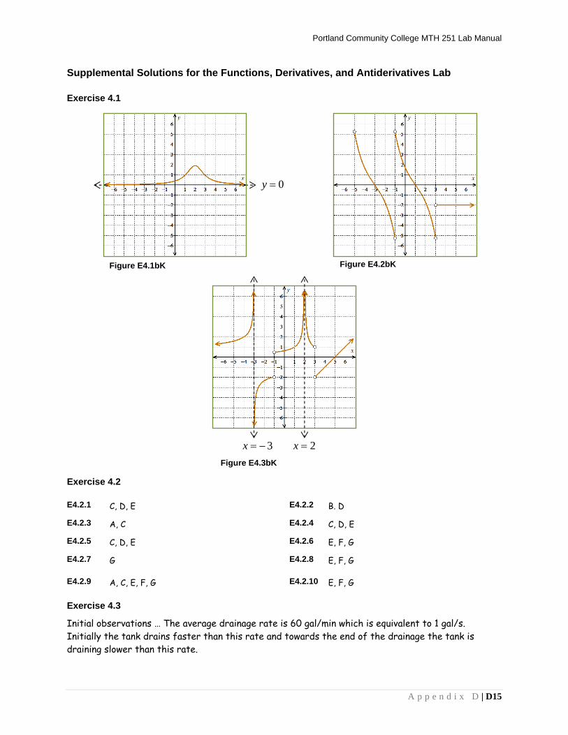
Portland Community College MTH 251 Lab Manual
A p p e n d i x D | D15
Supplemental Solutions for the Functions, Derivatives, and Antiderivatives Lab Exercise 4.1 Exercise 4.2 E4.2.1 C, D, E E4.2.2 B. D
E4.2.3 A, C E4.2.4 C, D, E
E4.2.5 C, D, E E4.2.6 E, F, G
E4.2.7 G E4.2.8 E, F, G
E4.2.9 A, C, E, F, G E4.2.10 E, F, G
Exercise 4.3
Initial observations … The average drainage rate is 60 gal/min which is equivalent to 1 gal/s. Initially the tank drains faster than this rate and towards the end of the drainage the tank is draining slower than this rate.
Figure E4.1bK
0y =
Figure E4.2bK
Figure E4.3bK
2x = 3x = −

Portland Community College MTH 251 Lab Manual
D16 | A p p e n d i x D
E4.3.1 The unit for 45V is gals and the unit for 45V is
gals
s.
Since the amount of water left in the tank is decreasing, the value of 45V cannot be
positive. Since 45 seconds is early in the drainage process the drainage rate is almost certainly greater than the average rate of 1 gal/s. Hence the most realistic value for
45V is 1.2 .
E4.3.2 The unit for 45R is gal
s
s and the unit for 45R is
gals
ss .
Since the flow rate decreases over time, the value of 45R cannot be positive. Since the
average flow rate over the 360 seconds is 1 gal/s, it is not believable that 45 seconds into the process the flow rate was decreasing at a rate 1 gal/s/s. Hence the most realistic value for 45R is 0.001 .
E4.3.3 This question is similar to question E4.5.2 with one key difference; because V is defined as the amount of water left in the tank, V has negative values. Since the value of V is getting closer to zero, V is increasing and, consequently, V cannot be negative. So the most realistic value for 45V is 0.001 .
Exercise 4.4
The answer to each question is ii.
Exercise 4.5
E4.5.1 Lisa is right. Maybe g is discontinuous at 3, but maybe it simply is pointy at 4.
E4.5.2 Janice is right although Lisa is pretty darn close to being right. The graph of g is basically the line 0y , but because g is nondifferentiable at 3, g has a hole at 4.
Exercise 4.6
E4.6.1 False: 0f t on 2,3 f decreasing on that interval
E4.6.2 True: f concave up on 2,3 f increasing on that interval
E4.6.3 False: 1 0f while 1 0f
E4.6.4 False: 6 1.7f , so the tangent line to f at 6 is a decreasing line.
E4.6.5 False: f is periodic; it would be increasing over each period, however (e.g.
0,4 , 4,8 ,

Portland Community College MTH 251 Lab Manual
A p p e n d i x D | D17
E4.6.6 False: ( )4 4.2f ′ ≈ ; if f were nondifferentiable at 4 then f ′ would have no value at 4.
E4.6.7 True
E4.6.8 True
E4.6.9 False: Although the “shape” if the antiderivatives is periodic, the antiderivatives clearly end up higher then they started after each interval of length 4.
E4.6.10 False: The amount of air in your lungs was increasing the entire two seconds.
E4.6.11 True
E4.6.12 True: Negative velocity corresponds to downward motion (because the “position” is decreasing when the velocity is negative).
Exercise 4.7 Table E4.1K
f ′′ f ′ f F Positive Increasing Negative Decreasing Constantly Zero Constant Positive Increasing Concave Up Negative Decreasing Concave Down Constantly Zero Constant Linear
Positive Increasing Concave Up Negative Decreasing Concave Down
Constantly Zero Constant Linear Exercise 4.8
E4.8.1 −1, 1, and 4 E4.8.2 nowhere
E4.8.3 ( )5,6− E4.8.4 ( )6, 3− − and ( )1,1−
E4.8.5 ( )4,6 E4.8.6 ( )3, 1− − , ( )1,4 , and ( )4,6
E4.8.7 ( )6, 5− − E4.8.8 there's no way to tell
E4.8.9 5− E4.8.10 4 2y x= − +

Portland Community College MTH 251 Lab Manual
D18 | A p p e n d i x D
Exercise 4.9
Exercise 4.10
Figure E4.6bK: F
Figure E4.7K f 2x =

Portland Community College MTH 251 Lab Manual
A p p e n d i x D | D19
Supplemental Solutions for the Derivative Formulas Lab Exercise 5.1
5.1.1 ( )
( )
6/11
5/11
11 5
16111
111
f x x
f x x
x
−
=
′ =
=
5.1.2 7
8
8
5
35
35
y t
dyt
dt
t
−
−
= −
=
=
5.1.3 ( )( )
1/3
2/3
3 2
12
44
y u u
y u u
u
−
=
′ =
=
5.1.4 ( )( ) 1
z e
z e
π
π
α α
α π α −
=
′ =
5.1.5 7/2
9/2
9
8
28
28
z t
dzt
dt
t
−
−
=
= −
= −
5.1.6 7/3
2
1/3
2/3
3 2
4
443
4
3
tT
t
t
dTt
dt
t
−
= ⋅
=
=
=
Exercise 5.2
5.2.1 ( ) ( )
( )( ) ( ) ( ) ( )( )( ) ( ) ( ) ( )( )( ) ( )2 2
5sin cos
5sin cos 5sin cos
5cos cos 5sin sin
5cos 5sin
y x x
dy d dx x x x
dx dx dx
x x x x
x x
= ⋅
= ⋅ + ⋅
= ⋅ + ⋅ −
= −
5.2.2
( )
( )
2
2 2
2
57
5 57 7
10 57 75 2
7
t
t t
t t
t
y t e
dy d dt e t e
dt dt dt
t e t e
t e t
= ⋅
⎛ ⎞= ⋅ + ⋅⎜ ⎟⎝ ⎠
= ⋅ +
+=
5.2.3 ( ) ( )
( ) ( ) ( ) ( )( )
( )
( )
4 ln
4 ln 4 ln
14 ln 4
4ln 4
F x x x
d dF x x x x x
dx dx
x xx
x
= ⋅
′ = ⋅ + ⋅
= ⋅ + ⋅
= +

Portland Community College MTH 251 Lab Manual
D20 | A p p e n d i x D
5.2.4 ( )
( ) ( ) ( )( )
( )
( )
2 1
2 1 2 1
1 2
2
21
2
sin
sin sin
12 sin1
2 sin1
z x x
dz d dx x x x
dx dx dx
x x xx
xx x
x
−
− −
−
−
= ⋅
= ⋅ + ⋅
= ⋅ + ⋅−
= +−
5.2.5 ( ) ( ) ( )
( ) ( ) ( ) ( ) ( )( )
( ) ( )( )
2 1
2 1 2 1
1 22
1
1 tan
1 tan 1 tan
12 tan 11
2 tan 1
T t t t
d dT t t t t t
dt dt
t t tt
t t
−
− −
−
−
= + ⋅
′ = + ⋅ + + ⋅
= ⋅ + + ⋅+
= +
5.2.6
( )
( )
( )( )
7
7 7
6 7
6
1 73
1 17 73 3
7 17 ln 7 73 3
7 7 ln 73
x
x x
x x
x
T x
dT d dx x
dx dx dx
x x
x x
= ⋅
⎛ ⎞= ⋅ + ⋅⎜ ⎟⎝ ⎠
= ⋅ + ⋅
+=
Exercise 5.3
5.3.1 ( )
( )( ) ( ) ( )
( )( )( )
( )( )
( )
2
2
2
2
41
4 1 4 1
1
4 1 4
1
4 1
1
4
1
eq
e
d de e e e
d dqe
e e e e
e
e e e
e
e
e
θ
θ
θ θ θ θ
θ
θ θ θ θ
θ
θ θ θ
θ
θ
θ
θ
θ θθ
=+
⋅ + − ⋅ +′ =
+
⋅ + − ⋅=
+
+ −=
+
=+

Portland Community College MTH 251 Lab Manual
A p p e n d i x D | D21
5.3.2 ( ) ( )
( )( )( ) ( ) ( )
( )( )
( )
( )( )
( )
4
4 4
24
4 3
8
3 3
8
3
8
5
2ln
2ln 2ln
12 2ln 4
2 8 ln
2 1 4ln
2 8ln
xu x
xd d
x x x xdx dxu x
x
x x xx
x
x x x
x
x x
xx
x
=
⋅ − ⋅′ =
⋅ ⋅ − ⋅=
−=
−=
−=
5.3.3
( )
( ) ( ) ( )( )
( )( )
( )
( )
1/2
2 3/2
1/2
1/2 3/2
3/2
3/2 3/2
23/2
3/2 1/2
23/2
1/2
23/2
23
3 5
3 5
13 5
1 3 5 1 3 5
3 5
90 3 5 1 52
3 5
95 2223 5
10 9
2 3 5
tF
t t
t
t t t
t t
d dt t t tdF dt dt
dt t t
t t t
t t
t
t t
t
t t
=−
=−
=−
⋅ − − ⋅ −=
−
⎛ ⎞⋅ − − ⋅ −⎜ ⎟⎝ ⎠=
−
−= ⋅
−
−=
−

Portland Community College MTH 251 Lab Manual
D22 | A p p e n d i x D
5.3.4 ( ) ( )( )
( )( )( ) ( ) ( ) ( )( )
( )( )( ) ( ) ( )
( )( )( ) ( ) ( ) ( )
( ) ( )( )
1
1 1
21
2 12 2
2 21
2 2 1
22 1
tantan
tan tan tan tan
tan
1sec tan tan1 1
1tan
1 sec tan tan
1 tan
xF x
x
d dx x x x
dx dxF xx
x x xx x
xx
x x x x
x x
−
− −
−
−
−
−
−
=
⋅ − ⋅′ =
⋅ − ⋅+ +
= ⋅+
+ −=
+
5.3.5 ( )
( )( ) ( ) ( ) ( )( )
( ) ( )
( )( )
( )
1
2
1 2 1 2
22
2 12
22
1
22
tan1
tan 1 tan 1
1
1 1 tan 21
1
1 2 tan
1
tP
t
d dt t t t
dP dt dtdt t
t t tt
t
t t
t
−
− −
−
−
=+
⋅ + − ⋅ +=
+
⋅ + − ⋅+
=+
−=
+
5.3.6 ( ) ( )
( ) ( ) ( )( ) ( ) ( )( )
( ) ( )( )( ) ( )( ) ( ) ( )( )( )
( ) ( )( )( ) ( )( )
( ) ( )( )
2
2
2
4sin 2cos
4 sin 2cos 4 sin 2cos
sin 2cos
0 sin 2cos 4 cos 2 sin
sin 2cos
4 cos 2sin
sin 2cos
y
d ddy d d
d
β β
β β β ββ β
β β β
β β β β
β β
β β
β β
=−
⋅ − − ⋅ −=
−
⋅ − − ⋅ − −=
−
− +=
−

Portland Community College MTH 251 Lab Manual
A p p e n d i x D | D23
Exercise 5.4 E5.4.1
( ) ( ) ( )( ) ( )( ) ( ) ( ) ( ) ( ) ( )
( ) ( ) ( ) ( ) ( )( ) ( ) ( ) ( )( )
( ) ( ) ( ) ( ) ( ) ( ) ( ) ( ) ( )
d d df x g x h x f x g x h x f x g x h x
dx dx dxd d
f x g x h x f x g x h x g x h xdx dx
f x g x h x f x g x h x f x g x h x
= +⎡ ⎤ ⎡ ⎤⎣ ⎦ ⎣ ⎦
⎡ ⎤′= + +⎡ ⎤⎣ ⎦ ⎢ ⎥⎣ ⎦′ ′ ′= + +
E5.4.2
( ) ( ) ( )
( ) ( ) ( ) ( ) ( ) ( ) ( ) ( )( ) ( ) ( ) ( )( )( ) ( ) ( ) ( ) ( ) ( ) ( ) ( )( )( ) ( ) ( ) ( ) ( ) ( )( )
2
2 2 2 2
2 2 2
2 2
sin cos
sin cos sin cos sin cos sin cos
2 sin cos sin cos cos cos sin sin
2sin cos sin cos cos sin
x
x x x x
x x x x
x
f x x e x x
d d d df x x e x x x e x x x e x x x e x x
dx dx dx dx
xe x x x e x x x e x x x e x x
xe x x x x x x x x x
=
′ = + + +
= + + + −
= + + −
Exercise 5.5
E5.5.1 ( )
( )
3 2
2 ; 02 1; 0
x xf x
x
x x x
f x x x
+=
= + ≠′ = + ≠
( )5 30f = and ( )5 11f ′ = So the tangent line to f at 5 passes through the point ( )5,30 and
has a slope of 11. The equation of this line is 11 25y x= − .
E5.5.2 ( )
( )( ) ( ) ( )
( )( )( )
( )
2
2
2
1
1 1
1
1 1 1
11
1
xh x
x
d dx x x x
dx dxh xx
x x
x
x
=+
⋅ + − ⋅ +′ =
+
⋅ + − ⋅=
+
=+
( )2 2h − = and ( )2 1h′ − = So the tangent line to h at 2− passes through the point ( )2,2−
and has a slope of 1. The equation of this line is 4y x= + .

Portland Community College MTH 251 Lab Manual
D24 | A p p e n d i x D
E5.5.3 ( )
( )
12 2
12 11 ; 12
xK x
x
x
x
h
+=
++
=+
= ≠ −
Since the graph of ( )y K x= is simply the horizontal line 0.5y = with a hole at 1− , the
tangent line to K at 8 must be the line with equation 0.5y = .
E5.5.4 ( )
( ) ( ) ( )
( )
1/3
1/3 1/3
2/3 1/3
1/3 2/3
2/3 2/3
23
3
3 3
33
11 3
x
x x
x x
x x
x
r x x e
d dr x x e x e
dx dx
x e x e
e x e x
x x
e x
x
−
= ⋅
′ = ⋅ + ⋅
= +
= + ⋅
+=
( )0 0r = and ( )0r′ has the form 10
. This form for ( )0r′ implies that r has a vertical tangent
line at 0 . So the tangent to r at 0 is the line 0x = .
Exercise 5.6 25
9/2 7/2211/2
7
4 22 994
99
dy d yy t t t tdt dtt
t
= = ==
=
E5.7.1 f ′ is positive over ( ), 8−∞ − and ( )2,∞ ; f ′ is negative over ( )8, 2− .
E5.7.2 f ′ is increasing over and ( )3,− ∞ ; f ′ is decreasing over ( ), 3−∞ − .
E5.7.3 f ′′ is positive over ( )3,− ∞ ; f ′′ is negative over ( ), 3−∞ − .
E5.7.4 ( ) 2 6 16f x x x′ = + −
( ) 2 6f x x′′ = +
Exercise 5.7
0y =
Figure E5.5.4K: 33 xy x e=
Figure E5.7.4Ka: ( )y f x′= Figure E5.7.4Kb: ( )y f x′′=

Portland Community College MTH 251 Lab Manual
A p p e n d i x D | D25
Exercise 5.8
E5.8.1 Over the interval [ ]0, 2π , ( ) 0g t′ = at 7 3 11, , ,
2 6 2 6π π π π
and .
E5.8.2 ( ) ( ) ( ) ( )
( ) ( ) ( )( ) ( ) ( ) ( )( )( ) ( ) ( ) ( ) ( )( ) ( ) ( )( ) ( )
3sin 3sin sin 5
3cos 3sin sin 3sin sin 0
3cos 3cos sin 3sin cos
3cos 6cos sin
3cos 1 2sin
g t t t t
d dg t t t t t t
dt dtt t t t t
t t t
t t
= + ⋅ −
′ = + ⋅ + ⋅ +
= + ⋅ + ⋅
= +
= +⎡ ⎤⎣ ⎦
So ( ) 0g t′ = where ( )cos 0t = or ( ) 1sin2
t = − . Over [ ]0, 2π , ( )cos 0t = at 2π
and
32π
. Over [ ]0, 2π , ( ) 1sin2
t = − at 76π
and 11
6π
. This comports with our answer to
problem E5.8.1
Exercise 5.9
( ) ( )( ) ( )
( ) ( )( ) ( ) ( ) ( )( )( ) ( ) ( ) ( )( )( ) ( ) ( ) ( )
( ) ( )( ) ( ) ( ) ( )( ) ( )( ) ( ) ( ) ( )( )
( )( ) ( ) ( ) ( )( ) ( )
sin 2
2sin cos
2sin cos 2sin cos
2 cos cos 2sin sin
2 cos cos 2sin sin
2 cos cos 2 cos cos 2sin sin 2sin sin
2sin cos 2 cos sin 2 cos
f x x
x x
d df x x x x x
dx dx
x x x x
x x x x
d d d df x x x x x x x x x
dx dx dx dx
x x x x x
=
= ⋅
′ = ⋅ + ⋅
= ⋅ + ⋅ −
= ⋅ − ⋅
⎡ ⎤ ⎡ ⎤′′ = ⋅ + ⋅ − ⋅ + ⋅⎢ ⎥ ⎢ ⎥⎣ ⎦ ⎣ ⎦⎡ ⎤= − ⋅ + − −⎣ ⎦ ( ) ( ) ( )
( ) ( )sin 2sin cos
8sin cos
x x x
x x
+⎡ ⎤⎣ ⎦= −
( ) 2f π′ = and ( ) 0f π′′ = So the tangent line to f ′ at π passes through the point ( ), 2π and has
a slope of 0 . The equation of this line is 2y = . Exercise 5.10
E5.10.1 ( ) ( ) ( )
( ) ( )( ) ( ) ( ) ( )( )( ) ( ) ( ) ( )
( ) ( ) ( ) ( ) ( )( )( ) ( )( )
4 4 4 4 4
39 289 46 29324,749
h x f x g x
d dh x f x g x f x g x
dx dxf x g x f x g x
h f g f g
=
′ = +
′ ′= +
′ ′ ′= +
= +
=

Portland Community College MTH 251 Lab Manual
D26 | A p p e n d i x D
E5.10.2 ( ) ( ) ( ) ( ) ( )
( ) ( )( ) ( ) ( ) ( )( ) ( )( ) ( ) ( ) ( )( )
( ) ( ) ( ) ( ) ( ) ( )( ) ( ) ( ) ( ) ( ) ( ) ( )
( )( ) ( )( ) ( )( )
2
2 2 2 2 2 2 2 2
10 11 2 7 37 4 58860
h x f x g x f x g x
d d d dh x f x g x f x g x f x g x f x g x
dx dx dx dx
f x g x f x g x f x g x
h f g f g f g
′ ′ ′= = +
⎡ ⎤ ⎡ ⎤′′ ′ ′ ′ ′= + + +⎢ ⎥ ⎢ ⎥⎣ ⎦ ⎣ ⎦′′ ′ ′ ′′= + +
′′ ′′ ′ ′ ′′= + +
= + +
=
E5.10.3 ( ) ( )( )
( )( )( ) ( ) ( ) ( )( )
( )( ) ( ) ( ) ( )
( )
( ) ( ) ( ) ( ) ( )( )
( )( ) ( )( )
2
2
2
2
3 3 3 33
3
126 15 87 2015
23
g xk x
f x
d dg x f x g x f x
dx dxk xf x
g x f x g x f x
f x
g f g fk
f
=
−′ =
⎡ ⎤⎣ ⎦′ ′−
=⎡ ⎤⎣ ⎦
′ ′−′ =
⎡ ⎤⎣ ⎦−
=
=
E5.10.4 ( ) ( )
( ) ( ) ( ) ( )( )
( ) ( )
( ) ( )
( ) ( ) ( )
( ) ( )( )
6
6 6
16 62
36
3 44 6 4 4
43 46
6 2 392
537
p x x f x
d dp x x f x x f x
dx dx
f x x f xx
f xx f x
x
fp f
=
′ = +
′= ⋅ +
′= +
′ ′= +
= +
=

Portland Community College MTH 251 Lab Manual
A p p e n d i x D | D27
E5.10.5 ( ) ( )( ) ( )
( ) ( )( ) ( ) ( ) ( )( )( ) ( )
( ) ( ) ( )( )( )
2
2
1 2 1 1
2 5 220
r x g x
g x g x
d dr x g x g x g x g x
dx dxg x g x
r g g
⎡ ⎤= ⎣ ⎦= ⋅
′ = +
′=
′ ′=
= −
= −
E5.10.6 ( ) ( ) ( )
( ) ( ) ( ) ( ) ( )( ) ( ) ( ) ( )( )( ) ( ) ( ) ( ) ( ) ( )
( ) ( ) ( ) ( ) ( ) ( ) ( )( )( ) ( )( ) ( )( )
2 2 2 2 2 2 2 2 2
4 11 2 7 11 2 4 37494
s x x f x g x
d d ds x x f x g x x f x g x x f x g x
dx dx dxf x g x x f x g x x f x g x
s f g f g f g
=
′ = + +
′ ′= + +
′ ′ ′= + +
= + +
=
E5.10.7 ( ) ( )
( )
( ) 2894 42 42892892894
2
F x x g F
x
F xx
= ′ ==
=′ =
E5.10.8 ( ) ( )
( )( )( ) ( ) ( )
( )( ) ( )
( )
2
2
x
x x
x
x x
x
x
f xT x
ed d
f x e f x edx dxT x
e
f x e f x e
e
e
=
⋅ − ⋅′ =
′ −=
=( ) ( )( )
x
f x f x
e
′ −
( ) ( )
x
x
e
f x f x
e
⋅′ −
=
(Continued on next page.)

Portland Community College MTH 251 Lab Manual
D28 | A p p e n d i x D
( )( ) ( )( ) ( ) ( )( ) ( )
( )( ) ( )( ) ( ) ( )( )
( )
2
2
x x
x
x x
x
x
d df x f x e f x f x e
dx dxT xe
f x f x e f x f x e
e
e
′ ′− ⋅ − − ⋅′′ =
′′ ′ ′− ⋅ − − ⋅=
=( ) ( ) ( ) ( )( )
x
f x f x f x f x
e
′′ ′ ′− − +
( ) ( ) ( )
( ) ( ) ( ) ( )
( )0
2
0 2 0 00
2 2 1 21
2
x
x
e
f x f x f x
ef f f
Te
⋅′′ ′− +
=
′′ ′− +′′ =
− − − +=
=

Portland Community College MTH 251 Lab Manual
A p p e n d i x D | D29
Supplemental Solutions for the Chain Rule Lab Exercise 6.1
( ) ( )3
3
3
3
33
x
x
x
df x e xdx
ee
′ = ⋅
= ⋅=
( ) ( ) ( )( )( )
2
2
3
3
3
3
3
3
x x
x x
x
x
dg x e edx
e e
e
e
′ = ⋅
= ⋅
=
=
( ) ( ) ( )3 3
3
ln
3
x
x
h x e e
e
′ = ⋅
=
Exercise 6.2
E6.2.1 ( ) 1k θ′ = over ,2 2π π⎛ ⎞−⎜ ⎟
⎝ ⎠
E6.2.2 Over ,2 2π π⎛ ⎞−⎜ ⎟
⎝ ⎠:
( )( )
( )( )
( )( ) ( ) ( )
( ) ( ) ( )
2
2 2
2
1 sin1 sin
1 cos (I used the identity cos sin 1 here.)cos
1= cos (As noted, cos 0 over , .)cos 2 21
dkd
θ θθθ
θ θ θθ
π πθ θθ
′ = ⋅−
= ⋅ + =
⎛ ⎞⋅ > −⎜ ⎟⎝ ⎠
=
E6.2.3 Over 3,
2 2π π⎛ ⎞⎜ ⎟⎝ ⎠
, ( )cos θ is constantly negative. By definition, u is never negative. So
over 3,
2 2π π⎛ ⎞⎜ ⎟⎝ ⎠
:
( )( )
( )
( ) ( )
2
1 coscos
1= coscos1
k θ θθ
θθ
′ = = ⋅
⋅−
= −
E6.2.4 2
k π⎛ ⎞′⎜ ⎟⎝ ⎠
is undefined. The function k is nondifferentiable at 2π
because it transitions
from a slope of 1 to a slope of 1− at that value.

Portland Community College MTH 251 Lab Manual
D30 | A p p e n d i x D
Exercise 6.3
E6.3.1 ( ) ( ) ( )( )( ) ( )
3
3
4
4
dg x f x f xdx
f x f x
′ ⎡ ⎤= ⋅⎣ ⎦
′⎡ ⎤= ⎣ ⎦
g′ is positive anywhere f and f ′ share the same sign. This occurs over ( )0, 2 and
( )3.2,∞ . (The left endpoint of the second interval is an approximation.)
E6.3.2 ( ) ( ) ( )( )( ) ( )
f x
f x
dr x e f xdx
e f x
′ = ⋅
′=
Since the factor of ( )f xe is always positive, ( )r x′ is positive anywhere ( )f x′ is positive.
This occurs over ( )2,∞ .
E6.3.3 ( ) ( ) ( )( )( ) ( ) ( )( ) ( ) ( )
( ) ( )1
f x
f x
f x
f x
dw x e f xdx
de f x xdx
e f x
e f x
−
−
−
−
′ = ⋅ −
′= − ⋅ −
′= − ⋅ −
′= − −
Since the factor of ( )f xe −− is always negative, ( )w x′ is positive anywhere ( )f x′ − is also
negative. Because the graph of ( )y f x′= is negative on the intervals ( ), 3−∞ − and ( )3, 2− ,
( )f x′ − is negative on the intervals ( )2,3− and ( )3,∞ . Ergo, ( )w x′ is positive over ( )2,3−
and ( )3,∞ . (Major high five if you figured that out on your own!)
E6.3.4 ( ) ( )
( ) ( ) ( )( )( )
( )
1
2
2
h x f x
dh x f x f xdx
f x
f x
−
−
⎡ ⎤= ⎣ ⎦
′ ⎡ ⎤= − ⋅⎣ ⎦
′= −
⎡ ⎤⎣ ⎦
( ) ( )( ) 2
2
33
3
04
0
fh
f
′ −′ − = −
⎡ ⎤−⎣ ⎦
= −
=
.
So, the function h is not nondifferentiable at 3− .

Portland Community College MTH 251 Lab Manual
A p p e n d i x D | D31
Exercise 6.4
E6.4.1 yes E6.4.2 no E6.4.3 no
E6.4.4 no E6.4.5 yes E6.4.6 yes
Exercise 6.5
E6.5.1 ( ) ( )( )
( ) ( )
( )
1
2
tan
1
1
1 11 2
12 1
f x x
df x xdxx
x x
x x
−=
′ = ⋅+
= ⋅+
=+
E6.5.2 ( ) ( )
( ) ( ) ( )( )( ) ( ) ( )( )( ) ( ) ( )( ) ( ) ( )
sin
sin
sin
sin
sin
sin
sin
sin
sin
sin
cos
cos
x
x
x
x
x
e
xe
xe
xe
x e
f x edf x e edx
de e xdx
e e x
x e +
=
′ = ⋅
= ⋅ ⋅
= ⋅ ⋅
=
E6.5.3 ( ) ( )( )( )
( )( )( )
( )( )( )
( )( )
1
2
2
sin cos
1 cos1 cos
1 sinsin
sinsin
f x x
df x xdxx
xx
xx
−=
′ = ⋅−
= ⋅ −
= −
E6.5.4 ( ) ( )( )( ) ( )( ) ( )( )
( )( ) ( ) ( ) ( )( )( )( ) ( ) ( ) ( )( )
( ) ( )( ) ( )( )
2
2
2
2
tan sec
sec sec sec
sec sec sec sec
sec sec 1 sec sec tan
sec sec sec 1 tan
f x x x
df x x x x xdx
d dx x x x x xdx dx
x x x x x x
x x x x x
=
′ = ⋅
⎛ ⎞= ⋅ ⋅ + ⋅⎜ ⎟⎝ ⎠
= ⋅ ⋅ + ⋅
= +

Portland Community College MTH 251 Lab Manual
D32 | A p p e n d i x D
E6.5.5 ( ) ( ) ( )( )( ) ( )( ) ( )( ) ( ) ( )( )( )
( ) ( )( ) ( ) ( )( ) ( )( ) ( )( )( ) ( )( ) ( ) ( )( ) ( )( ) ( ) ( )
( ) ( )( ) ( ) ( ) ( )( )
2
2
2
tan sec sec
tan sec sec tan sec sec
sec sec sec tan sec sec tan sec sec
sec sec sec tan sec sec tan sec sec tan
sec sec sec sec tan tan sec
f x x x
d df x x x x xdx dx
dx x x x x xdx
x x x x x x x
x x x x x
=
′ = ⋅ + ⋅
= + ⋅
= +
⎡ ⎤= +⎣ ⎦
E6.5.6 ( ) ( )( )( )( )
( ) ( )( ) ( )( )( )( ) ( ) ( )
( )( ) ( )( )( )
223
2/32
1/32 2
1/32 2 2
1/32 2
2
23
sin
sin
2 sin sin32 sin cos32 sin cos 234 cos
3 sin
f x x
x
df x x xdx
dx x xdx
x x x
x x
x
−
−
−
=
=
′ = ⋅
= ⋅ ⋅
= ⋅
=
E6.5.7 ( ) ( )
( ) ( ) ( ) ( )( )( )( ) ( ) ( )( )
( ) ( ) ( )( ) ( ) ( )( )
2
22
2
2
4 sin
4 sin 4 sin
4 sin 4 2sin sin
4sin 8 sin cos
4sin sin 2 cos
f x x xd df x x x x xdx dx
dx x x xdx
x x x x
x x x x
=
′ = ⋅ + ⋅
= ⋅ + ⋅ ⋅
= +
= +
E6.5.8 ( ) ( )( )( ) ( )( )
ln ln
ln ln ln
f x x x
x x
=
= +
( ) ( ) ( )( )
( )( )
( )
1 1 lnln
1 1 1ln
ln 1ln
df x xx x dx
x x x
xx x
′ = + ⋅
= + ⋅
+=
E6.5.9 ( )
( ) ( )( ) ( ) ( )( ) ( )
5ln
ln 5 ln
ln 5 ln ln
ln 5 ln
x
x
x
f xxe
x e
x e
x x
⎛ ⎞= ⎜ ⎟
⎝ ⎠
= −
⎡ ⎤= − +⎣ ⎦= − −
( ) 10 1
1
f xx
xx
′ = − −
+= −

Portland Community College MTH 251 Lab Manual
A p p e n d i x D | D33
E6.5.10 ( ) ( )( )( )( )( )
( )( )
( ) ( )( )
( ) ( )( )
23
1/32
2
2
2ln tan
2ln tan
12 ln tan3
2 ln ln tan32 ln 2ln tan3
f x x x
x x
x x
x x
x x
=
=
= ⋅
⎡ ⎤= +⎣ ⎦
⎡ ⎤= +⎣ ⎦
( ) ( ) ( )( )
( ) ( )
( ) ( )( )( )
2
2
2 1 12 tan3 tan
2 1 2 sec3 tan
2 tan 2 sec
3 tan
df x xx x dx
xx x
x x xx x
⎡ ⎤′ = + ⋅ ⋅⎢ ⎥
⎢ ⎥⎣ ⎦⎡ ⎤
= + ⋅⎢ ⎥⎢ ⎥⎣ ⎦
+=
E6.5.11 ( )
( ) ( )( )( )
2
1/22
ln2
ln ln 2
12 ln 22
x
x
ef xx
e x
x x
+
+
⎛ ⎞= ⎜ ⎟⎜ ⎟+⎝ ⎠
= − +
= + − +
( ) ( )
( )
( )
1 11 0 22 2
1 11 12 2
2 4 12 22 3
2 2
df x xx dx
xx
xxx
′ = + − ⋅ ⋅ ++
= − ⋅ ⋅+
+ −=++=+
E6.5.12 ( ) ( )( ) ( )
( )1
1
ln
1
1 0
e
ee
ee
e
e
f x x e
df x x ex e dx
e xx ee xx e
−
−
= +
′ = ⋅ ++
= ⋅ ++
=+
E6.5.13 ( ) ( )( )
( ) ( ) ( )( )( ) ( ) ( ) ( )( ) ( )
4
4
3
3
4
sec
sec
4 sec sec
4sec sec tan
4sec tan
x
x
x x
x x x x
x x x
f x e
e
df x e edx
de e e edx
e e e
=
⎡ ⎤= ⎣ ⎦
⎡ ⎤′ = ⋅⎣ ⎦
= ⋅ ⋅
=
E6.5.14 ( ) ( )( )
( )( )
1
2
sec
1
1
1
x
x
x x
x
f x e
df x edxe e
e
−=
′ =−
=2 1
x
xe
e⋅
−
2
11xe
=−
E6.5.15 ( )
( )( ) ( ) ( ) ( )
( ) ( )
1/2
1/2 1/2 1/2
1/2 1/2 3/2
3
1csc
csc
csc cot
1csc cot2
1 1csc cot
2
f xx
x
df x x x xdx
x x x
x xx
−
− − −
− − −
⎛ ⎞= ⎜ ⎟⎝ ⎠
=
′ = − ⋅
= − ⋅−
⎛ ⎞ ⎛ ⎞⎜ ⎟ ⎜ ⎟⎝ ⎠ ⎝ ⎠=

Portland Community College MTH 251 Lab Manual
D34 | A p p e n d i x D
E6.5.16 ( ) ( )( )
( ) ( ) ( )( )( )
1csc
sin
cos
1cos2
cos
2
f xx
x
df x x xdx
xx
x
x
=
=
′ = ⋅
= ⋅
=
E6.5.17 ( ) ( )
( )
( )( )
( )
1
1
2
2
2
tan 22
1 tan 221 1 22 1 21 1 22 1 4
11 4
xf x
x
df x xdxx
x
x
−
−
=
=
′ = ⋅ ⋅+
= ⋅ ⋅+
=+
E6.5.18 ( )
( ) ( )
3
3 3
2 3
2 3
2
sin3
sin sin3 3
3 sin cos3 3 3
13 sin cos3 3 3
9sin cos3 3
3
xf x x
d x d xf x x xdx dx
x x d xx xdx
x xx x
x xx x
⎛ ⎞= ⎜ ⎟⎝ ⎠
⎛ ⎞⎛ ⎞ ⎛ ⎞′ = ⋅ + ⋅ ⎜ ⎟⎜ ⎟ ⎜ ⎟⎝ ⎠ ⎝ ⎠⎝ ⎠
⎛ ⎞ ⎛ ⎞ ⎛ ⎞= ⋅ + ⋅ ⋅⎜ ⎟ ⎜ ⎟ ⎜ ⎟⎝ ⎠ ⎝ ⎠ ⎝ ⎠⎛ ⎞ ⎛ ⎞= + ⋅⎜ ⎟ ⎜ ⎟⎝ ⎠ ⎝ ⎠
⎛ ⎞⎛ ⎞ ⎛ ⎞+⎜ ⎟ ⎜ ⎟⎜ ⎟⎝ ⎠ ⎝ ⎠⎝ ⎠=
E6.5.19 ( )
( )
7
7/2
5/2
5
43
43
4 723
143
f x
x
x
f x x
x
=
=
′ = ⋅
=
E6.5.20 ( )
( )( ) ( )
( )
( ) ( )
( )
( )
2
2
2
2
2
2
1
1
1
x
x x
x x
x x
x x
x
x e
x e x e
x e x x e
x e x x x e
x e x x x e
x e x x
ef xx
d de x e xdx dxf x
xde xe x edx
xd de x e x e x edx dx
xe e x e x e
xe xe x e
x
=
⋅ −′ =
⋅ ⋅ − ⋅=
⎛ ⎞⋅ ⋅ + ⋅ ⋅ −⎜ ⎟⎝ ⎠=
⋅ + ⋅ ⋅ −=
+ −=

Portland Community College MTH 251 Lab Manual
A p p e n d i x D | D35
E6.5.21 ( )
( ) ( ) ( )( )
( )
2
2 2
2 2
2 2
2
2
2
2
1
1
xe
xe xe
xe xe
xe xe
xe
f x x ed df x x e x edx dx
de x e x edx
e x e e
e x e
=
′ = ⋅ + ⋅
= ⋅ + ⋅ ⋅
= + ⋅
= +
E6.5.22 ( ) ( ) ( )( )
( )( )( )
( )( )
( )( ) ( )( )
( ) ( )( ) ( )( ) ( )( ) ( )( )
( ) ( )( )
( )
( ) ( )( )
5 3 3/2
353
94 1/2
3
1sin sin 4 sin sin sin sin2sin
1 14sin cos cossin sin 2 sinsin sin
cos 8 sin 1sin sin
2 sin
d dx x f x x x x xf x dx dxxx x xx x x
x xx x
x xx
−
−
− ′ = ⋅ + ⋅=
= + ⋅ ⋅= −
⎡ ⎤+⎣ ⎦= − =
E6.5.23 ( ) ( ) ( )( ) ( ) ( ) ( ) ( )( ) ( ) ( ) ( )( )
( ) ( ) ( ) ( ) ( ) ( )( ) ( )( ) ( ) ( ) ( ) ( ) ( )( ) ( ) ( ) ( ) ( ) ( )
2
2 2 2
2 2 2 2
2 2 2
2 2 2 2
4 sin cos
4 sin cos 4 sin cos 4 sin cos
4 sin cos 4 cos cos 4 sin sin
4sin cos 4 cos cos 4 sin sin 2
4sin cos 4 cos cos 8 sin sin
f x x x x
d d df x x x x x x x x x xdx dx dx
dx x x x x x x x xdx
x x x x x x x x x
x x x x x x x x
=
′ = ⋅ + ⋅ ⋅ + ⋅
= ⋅ + ⋅ ⋅ + ⋅ − ⋅
= + − ⋅
= + −
E6.5.24 ( ) ( )( )( ) ( )( ) ( )( )
( )( ) ( ) ( ) ( )( )( )( )( ) ( ) ( ) ( )( )
( )( ) ( ) ( ) ( )( )( ) ( )( ) ( ) ( )
2
2 2
22 2
2 2
2 2
2
sin cos
cos cos cos
cos cos cos cos
cos cos 1 cos 2cos cos
cos cos cos 2 cos sin
cos cos cos cos 2 sin
f x x x
df x x x x xdx
d dx x x x x xdx dx
dx x x x x xdx
x x x x x x
x x x x x x
=
′ = ⋅
⎡ ⎤= ⋅ ⋅ + ⋅⎢ ⎥⎣ ⎦⎡ ⎤= ⋅ ⋅ + ⋅ ⋅⎢ ⎥⎣ ⎦⎡ ⎤= ⋅ + ⋅ −⎣ ⎦
⎡ ⎤= ⋅ −⎣ ⎦

Portland Community College MTH 251 Lab Manual
D36 | A p p e n d i x D

Portland Community College MTH 251 Lab Manual
A p p e n d i x D | D37
Supplemental Solutions for the Implicit Differentiation Lab Exercise 7.1
( )
( ) ( )
( ) ( ) ( )( )
( ) ( ) ( )
( ) ( ) ( ) ( )
( ) ( )
( ) ( ) ( )
( ) ( )
2
2
sin
sin
sin sin
1 sin cos
sin cos
sin cos 1
sin cos cos
sin cos 1 cos
x x y yd dx x y ydx dx
d d dyx x y x x ydx dx dx
d dyx y x x y x ydx dx
d d dyx y x x y x y x ydx dx dx
dy dyx y x x y y xdx dxdy dyx y x y x y x x ydx dx
x y x y x y x
=
=⎡ ⎤⎣ ⎦
⋅ + ⋅ =
⋅ + ⋅ ⋅ =
⎡ ⎤+ ⋅ ⋅ + ⋅ =⎢ ⎥⎣ ⎦⎡ ⎤+ ⋅ ⋅ + ⋅ =⎢ ⎥⎣ ⎦
+ + =
+ = − ( )
( ) ( )( )2
sin cos1 cos
dyx ydx
x y x y x y dyx x y dx
⎡ ⎤⎣ ⎦
+=
−
Since we’re looking for points on the y-axis, we know that the y-coordinates are zero. A necessary element for the tangent line to be vertical is that the denominator of the derivative formula evaluates to zero (otherwise the tangent line would have a value for its slope). Putting this together gives us:
( )2 21 cos 0 0 1 0 1x x x x− ⋅ = ⇒ − = ⇒ = ±
So the x-coordinates are 1 and 1− . Exercise 7.2
( )( ) ( )( ) ( )
( ) ( )( ) ( )
( )
2 2
2 2
1, 1
ln
ln ln
2 ln 2 ln
2 ln 2 ln
1 12 2 1
2 21 1
21
2 1
13
x y x y
x y x y
x y x yd dx y x ydx dx
dy dyx y dx dx
dyy dx x
dy xdx
ydydx −
= +
+ = +
+ = +
+ = +
⋅ + ⋅ = +
⎛ ⎞− = −⎜ ⎟⎝ ⎠
−=
−
=
Figure E7.2K: ( )2 2ln x y x y= +
The slope of the tangent line is 13
and the line passes through the
point ( )1, 1− , so the equation of the tangent line is 1 43 3
y x= − .

Portland Community College MTH 251 Lab Manual
D38 | A p p e n d i x D
Exercise 7.3 ( ) ( ) ( ) ( )ln ln ln lnx xy x y x y x x= ⇒ = ⇒ = ⋅
( )( ) ( )( )
( ) ( ) ( )( )
( )
( )( )
( )( )
ln ln
1 ln ln
1 11 ln
ln 1
ln 1x
d dy x xdx dx
dy d dx x x xy dx dx dx
dy x xy dx x
dy y xdxdy x xdx
= ⋅
= ⋅ + ⋅
= ⋅ + ⋅
= +
= +
Exercise 7.4 7.4.1
( )
( ) ( )
( ) ( )( ) ( )
( ) ( ) ( )( ) ( )
( )( ) ( ) ( )( ) ( )
( ) ( )( ) ( )
( ) ( )
( )
1/2
sin
1
sinln ln
1
ln ln sin ln 1
1ln ln ln sin ln 12
1ln ln ln sin ln 12
1 1 1 1 1sin 1sin 2 1
1 1 1 1cos 1sin 2 1
sin
1
x xy
x
x xy
x
y x x x
y x x x
d dy x x xdx dx
dy d dx xy dx x x dx x dx
dy y xdx x x x
x xdydx x
=−
⎛ ⎞= ⎜ ⎟⎜ ⎟−⎝ ⎠
⎡ ⎤= − −⎣ ⎦
= + − −
⎡ ⎤= + − −⎢ ⎥⎣ ⎦
= + ⋅ − ⋅ ⋅ −−
⎡ ⎤= + ⋅ − ⋅ ⋅⎢ ⎥−⎢ ⎥⎣ ⎦
=−
( ) ( )1 1cot
2 1x
x x⎡ ⎤
+ −⎢ ⎥−⎢ ⎥⎣ ⎦

Portland Community College MTH 251 Lab Manual
A p p e n d i x D | D39
7.4.2
( )
( )( )
( ) ( ) ( )( )( ) ( )( )( ) ( )
( ) ( )( ) ( )
2
4 54
2
4 54
2 4 54
4 5/4
sin
ln lnsin
ln ln ln sin
ln 2 ln sin ln
5ln 2 4ln sin ln4
x
x
x
eyx x
eyx x
y e x x
y x x x
y x x x
=
⎛ ⎞⎜ ⎟=⎜ ⎟⎝ ⎠
= −
⎡ ⎤= − +⎢ ⎥⎣ ⎦
= − −
( )( ) ( )( ) ( )
( ) ( )( )
( ) ( )
( )( )
2
44 5
5ln 2 4ln sin ln4
1 1 5 12 4 sinsin 4
1 52 4 cossin 4
52 4cot4sin
x
d dy x x xdx dx
dy d xy dx x dx x
dy y xdx x x
dy e xdx xx x
⎡ ⎤= − −⎢ ⎥⎣ ⎦
= − ⋅ ⋅ − ⋅
⎡ ⎤= − ⋅ ⋅ −⎢ ⎥
⎢ ⎥⎣ ⎦⎡ ⎤
= − −⎢ ⎥⎣ ⎦
7.4.3
( )( )
( ) ( )( )
( ) ( )( ) ( )( )( ) ( )( ) ( ) ( )( )( ) ( )( ) ( ) ( )( )
( )( ) ( )( ) ( ) ( )( )
( ) ( )( ) ( ) ( )( )
( ) ( )
3
5
3
5
3 5
3 5
3
3
33
333
ln 4
ln
ln 4ln ln
ln
ln ln ln 4 ln ln
ln ln ln 4 ln ln ln
ln ln ln 4 5 ln ln ln
ln ln ln 4 5 ln ln ln
1 1 1 1ln 4 5 lnlnln 4
1 1 1 44ln 4
xy
x x
xy
x x
y x x x
y x x x
y x x x
d dy x x xdx dx
dy d dx xy dx dx x x dxx
dy d xy dx dxxx
=
⎛ ⎞⎜ ⎟=⎜ ⎟⎝ ⎠
= −
⎡ ⎤= − +⎣ ⎦
= − −
⎡ ⎤= − −⎣ ⎦
= ⋅ − ⋅ − ⋅
= ⋅ ⋅ −( )
( ) ( )
( ) ( )
( )( ) ( ) ( )
233
3
3
5 3
5 1 1ln
1 1 1 5 112ln4ln 4
3 5 1lnln 4
ln 4 3 5 1lnln ln 4
x x x
dy xy dx x x xxx
dy ydx x x xx x
xdydx x x xx x x x
− ⋅
= ⋅ ⋅ − −
⎡ ⎤⎢ ⎥= − −⎢ ⎥⎣ ⎦
⎡ ⎤⎢ ⎥= − −⎢ ⎥⎣ ⎦

Portland Community College MTH 251 Lab Manual
D40 | A p p e n d i x D

Portland Community College MTH 251 Lab Manual
A p p e n d i x D | D41
Supplemental Solutions for the Related Rates Lab Exercise 8.1 Define x to be the elevation (ft) of the balloon t seconds after the balloon begins to rise and y to be the distance (ft) between the observer and the balloon at the same instant. The relation equation is 2 2 2300x y . The rate equation is:
2 290000 2 2d d dx dyx y x y
dt dt dt dt
When the elevation of the balloon is 400 feet:
400x , 500y (from the Pythagorean Theorem), and 10dx
dt
Substituting these values into the rate equation we get:
2 400 10 2 500 8dy dy
dt dt
So the distance between the observer and the balloon is increasing at a rate of 8 ft/s at the instant the elevation of the balloon is 400 feet.
x y
300 Figure E8.1K: Variable Diagram

Portland Community College MTH 251 Lab Manual
D42 | A p p e n d i x D
Exercise 8.2 Define x to be the vertical distance (ft) between the tip of the arm and the horizontal position of the arm t seconds after gate begins to close and to be the angle of elevation (rad) at the pivot point at the same instant in time.
The relation equation is sin28x .
The rate equation is: 1sin cos28 28
d d x d dx
dt dt dt dt
At the instant the angle at the pivot point is 30O:
6 and raddeg6 s 180 deg
rads30
d
dt
Substituting these values into the rate equation we have:
1cos 2.546 30 28
dx dx
dt dt
So at the instant the angle of elevation of the arm is 30O, the tip of the arm is approaching the ground at a rate of about 2.54 ft/s.
x
28
Figure E8.2K: Variable Diagram

Portland Community College MTH 251 Lab Manual
A p p e n d i x D | D43
Exercise 8.3 Define V to be the volume of soda (cm3) that remains in Jimbo’s cup t seconds after he commences to sip and h to be the height of the soda in the cup (cm) at that very same instant. The volume formula for a right circular cone is
2
3V r h
where V represents the volume of the cone,
h represents the height of the cone, and r represents the radius at the top of the cone. Since neither of our defined variable is a radius, we need to purge that variable from our volume formula.
From the similar triangles shown in Figure E8.3K we have, 5
10 2r h
rh .
Substituting the expression 2h
for r in the volume formula we get our relation equation:
2
2 3
3 3 2 12h
V r h V h V h
Our rate equation is: 3 2
12 4d d dV dh
V h hdt dt dt dt
At the instant there are 100 cm3 of soda remaining in the cup:
3 31200100
12h h
; also, 0.25dV
dt
Substituting these values into our rate equation we get:
2
312000.25 0.006
4dh dh
dt dt
So at the instant there are 100 cm3 of soda remaining in the cup, the height of the soda in the cup is decreasing at a rate of about 0.006 cm/s. Somebody needs to tell Jimbo to put some juice into his sipping rate!
h
r
5
10
FigureE8.3K: Similar Triangles

Portland Community College MTH 251 Lab Manual
D44 | A p p e n d i x D
Exercise 8.4 Define V to be the volume of the snowball (cm3) and A to be the surface area of the snowball (cm2) t minutes after the snowball began to melt. The volume and surface area formulas for a sphere in terms of the radius, r, of the sphere are,
respectively, 343
V r and 24A r . Solving the volume formula for r we have
1/31/3
1/3
34
r V
and substituting the resultant expression into the area formula we have our relation equation:
21/3
2 1/3 2/331/3
34 4 364
A r A V A V
This gives us our rate equation:
2/3 1/33 3 32 2 3636 363 3
d d dA dV dA dVA V V
dt dt dt dt dt V dt
When the radius of the snowball is 6 cm:
34 63288
V
and 25dV
dt
Substituting these values into our rate equation we get:
3
13
2 36 253 288
8
dA
dt
So at the instant the radius of the snowball is 6 cm, the surface area of the snowball is decreasing at the rate of 1
38 cm2/minute.

Portland Community College MTH 251 Lab Manual
A p p e n d i x D | D45
Supplemental Solutions for the Critical Numbers and Graphing from Formulas Lab Exercise 9.1
E9.1.1 ( ) ( )2 2
2 2
2 2 2 2
2 2 2 2
cosh sinh2 2
2 24 42 2
4441
t t t t
t t t t
t t t t
e e e et t
e e e e
e e e e
− −
− −
− −
⎛ ⎞ ⎛ ⎞+ −− = −⎜ ⎟ ⎜ ⎟⎝ ⎠ ⎝ ⎠
+ + − += −
+ + − + −=
=
=
E9.1.2 For ( ) ( )coshf t t= and ( ) ( )sinhg t t= :
( ) ( )
( )
( )( )
12
1 1212sinh
t t
t t
t t
df t e edt
e e
e e
t
−
−
−
⎛ ⎞′ = +⎜ ⎟⎝ ⎠
= + ⋅−
= −
=
( ) ( )
( )
( )( )
12
1 1212cosh
t t
t t
t t
dg t e edt
e e
e e
t
−
−
−
⎛ ⎞′ = −⎜ ⎟⎝ ⎠
= − ⋅−
= +
=
It follows that ( ) ( )coshf t t′′ = and ( ) ( )sinhg t t′′ =
E9.1.3 The domains of both f and g are ( ),−∞ ∞ . f ′ and g′ are both always defined, so the
only issue is when ( ) 0f t′ = and when ( ) 0g t′ = .
( )
( )2
0 02
1
1
1
t t
t t
tt
t
t
e ef t
e e
ee
e
e
−
−
−′ = ⇒ =
⇒ =
⇒ =
⇒ =
⇒ = ±
te is never negative and 1te = when 0t = .
Therefore, the only critical number for ( ) ( )coshf t t= is 0 .
( ) 0 02
t t
t t
e eg t
e e
−
−
+′ = ⇒ =
⇒ = −
Since real number powers of e are always positive, te never equals te−− . Therefore,
( ) ( )sinhg t t= has no critical numbers.

Portland Community College MTH 251 Lab Manual
D46 | A p p e n d i x D
E9.1.4 Table 9.1.1K: Sign analysis for ( )sinh t
Interval ( )sinh t
( ),0−∞ negative
( )0,∞ positive
Table 9.1.2K: Sign analysis for ( )cosh t
Interval ( )cosh t
( ),−∞ ∞ positive
( ) ( )sinhf t t= , ( ) ( )coshf t t′ = and ( ) ( )sinhf t t′′ = . So based upon the signs shown in
tables 9.1.1K and 9.1.2K we can conclude that ( ) ( )sinhf t t= is always increasing, concave
down on ( ),0−∞ and concave up on ( )0,∞ . We should note that the point ( )0,0 is an
inflection point on f and that the slope of f at that point is ( )cosh 0 which is 1.
( ) ( )coshg t t= , ( ) ( )sinhg t t′ = , and ( ) ( )coshg t t′′ = . So based upon the signs shown in
tables 9.1.1K and 9.1.2K we can conclude that ( ) ( )coshg t t= is decreasing on ( ),0−∞ ,
increasing on ( )0,∞ , and always concave up. We should note that the point ( )0,1 is a local
minimum point on the graph of g and that g has a horizontal tangent line at that point.
E9.1.5 Each of the hyperbolic limits are based upon these four basic limits: lim t
te
→ ∞= ∞ ,
lim 0t
te
→ −∞= , lim 0t
te−
→ ∞= , and lim t
te−
→ −∞= ∞
( )lim cosh lim2
t t
t t
e et−
→ −∞ → −∞
+=
= ∞ ( )lim sinh lim
2
t t
t t
e et−
→ −∞ → −∞
−=
= − ∞
( )lim cosh lim2
t t
t t
e et−
→ ∞ → ∞
+=
= ∞ ( )lim sinh lim
2
t t
t t
e et−
→ ∞ → ∞
−=
= ∞
E9.1.6 Figure 9.1.1K: ( )sinhy t= Figure 9.1.2K: ( )coshy t=

Portland Community College MTH 251 Lab Manual
A p p e n d i x D | D47
E9.1.7 ( ) ( )( )
sinhtanh
cosh
2
2
t t
t t
t t
t t
tt
t
e e
e e
e ee e
−
−
−
−
=
−
=+
−=+
( ) ( )1sech
cosh2
t t
tt
e e−
=
=+
( ) ( )1csch
sinh2
t t
tt
e e−
=
=−
( ) ( )1coth
tanht t
t t
tt
e ee e
−
−
=
+=−
E9.1.8 A good guess for ( )( )tanhd tdt
would be ( )sech t . Checking it out …
( )( )
( )( ) ( )( )( )
( )( ) ( )( )( )
( )( )
( )
( )
2
2
2 2 2 2
2
2
2
2
tanh
1 1
1 1 1 1
4
2
sech
t t
t t
t t t t t t t t
t t
t t t t t t t t
t t
t t t t
t t
t t
t t
d d e etdt dt e e
e e e e e e e e
e e
e e e e e e e e
e e
e e e e
e e
e e
e e
t
−
−
− − − −
−
− − − − −
−
− −
−
−
−
⎛ ⎞−= ⎜ ⎟+⎝ ⎠
− ⋅− + − − + ⋅−=
+
+ + − − −=
+
+ + + − − − +=
+
=+
⎡ ⎤= ⎢ ⎥+⎣ ⎦=
E9.1.9 ( )2
2t tf t
e e−
⎡ ⎤′ = ⎢ ⎥+⎣ ⎦ is always positive so f is always increasing.
( )0 0f = and ( )0 1f ′ =
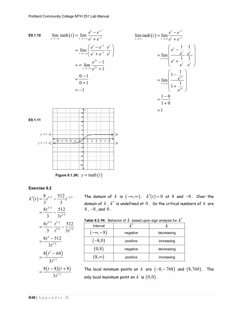
Portland Community College MTH 251 Lab Manual
D48 | A p p e n d i x D
E9.1.10 ( )
2
2
lim tanh lim
lim
1lim1
0 10 1
1
t t
t tt t
t t t
t t tt
t
tt
e ete e
e e ee e e
ee
−
−→ −∞ → −∞
−
−→ −∞
→ −∞
−=+
⎛ ⎞−= ⋅⎜ ⎟+⎝ ⎠−= =+
−=+
= −
( )
2
2
lim tanh lim
1 1
lim 1 1
11lim 11
1 01 01
t t
t tt t
tt t
t tt t
t
t
t
e ete e
ee e
ee e
e
e
−
−→ ∞ → ∞
→ ∞
→ ∞
−=+
⎛ ⎞−⎜ ⎟= ⋅⎜ ⎟
⎜ ⎟+⎝ ⎠⎛ ⎞−⎜ ⎟
= ⎜ ⎟⎜ ⎟+⎝ ⎠
−=+
=
E9.1.11 Exercise 9.2
( )
( )
( )( )
5/3 1/3
5/3
1/3
5/3 1/3
1/3 1/3
2
1/3
2
1/3
1/3
8 5123 38 512
3 38 512
3 38 512
3
8 643
8 8 83
k t t t
tt
t tt t
tt
tt
t tt
−′ = −
= −
= ⋅ −
−=
−=
− +=
The domain of k is ( ),−∞ ∞ . ( ) 0k t′ = at 8 and 8− . Over the
domain of k , k′ is undefined at 0 . So the critical numbers of k are 8 , 8− , and 0 . Table 9.2.1K: Behavior of k based upon sign analysis for k′
Interval k′ k
( ), 8−∞ − negative decreasing
( )8,0− positive increasing
( )0,8 negative decreasing
( )8,∞ positive increasing
The local minimum points on k are ( )8, 768− − and ( )8,768 . The
only local maximum point on k is ( )0,0 .
1y =
1y = −
Figure 9.1.3K: ( )tanhy t=

Portland Community College MTH 251 Lab Manual
A p p e n d i x D | D49
Exercise 9.3
( ) ( ) ( ) ( )( ) ( )( )
2cos sin cos
cos 1 2sin
f x x x x
x x
′ = ⋅− +
= −
The domain of f has been restricted to [ ]0,2π . Over [ ]0,2π , ( )cos 0x = at 2π
and 32π
and
( ) 1sin2
x = at 6π
and 56π
. So over the restricted domain ( ) 0f x′ = at 2π
, 32π
, 6π
, and 56π
.
f ′ is never undefined. So the critical numbers of f are 6π
, 2π
, 56π
, and 32π
.
Table 9.3.1K: Behavior of f based upon sign analysis for f ′
Interval f ′ f
0,6π⎛ ⎞
⎜ ⎟⎝ ⎠
positive increasing
,6 2π π⎛ ⎞⎜ ⎟⎝ ⎠
negative decreasing
5,2 6π π⎛ ⎞⎜ ⎟⎝ ⎠
positive increasing
5 3,6 2π π⎛ ⎞
⎜ ⎟⎝ ⎠
negative decreasing
3 ,22π π⎛ ⎞
⎜ ⎟⎝ ⎠
positive increasing
Exercise 9.4
( ) ( )( ) ( )( )( )
( )
3 2
23
3 3 2
6
3 2
6
2
6
4
1 9 3
3 27
2 27
2 27
2 27
t t tg t
t
t t tt
t tt
t tt
tt
− +′ =
− −=
− −=
− −=
− −=
( ) ( )( ) ( )( )( )
( )
( )
( )
4 3
24
4 4 3
8
4 3
8
3
8
5
5
2 2 27 4
2 8 108
6 108
2 3 54
2 3 18
6 18
t t tg t
t
t t tt
t tt
t tt
tt
tt
− − − −′′ =
− + +=
+=
+=
⋅ +=
+=
Over [ ]0,2π the local minimum points
on f are ,12π⎛ ⎞⎜ ⎟⎝ ⎠
and 3 , 12π⎛ ⎞−⎜ ⎟
⎝ ⎠ and the
local maximum points are 5,
6 4π⎛ ⎞⎜ ⎟⎝ ⎠
and
5 5,6 4π⎛ ⎞
⎜ ⎟⎝ ⎠
.

Portland Community College MTH 251 Lab Manual
D50 | A p p e n d i x D
( ) 0g t′′ = at 18− and ( )g t′′ is undefined at 0 .
Table 9.4.1K: Behavior of g based upon sign analysis for g′′
Interval g′′ g
( ), 18−∞ − positive concave up
( )18,0− negative concave down
( )0,∞ positive concave up
The only inflection point on g is 118,
648⎛ ⎞−⎜ ⎟⎝ ⎠
; g has a vertical asymptote at 0 .
Exercise 9.5 E9.5.2
( ) ( )( ) ( ) ( )( )( )
( ) ( ) ( )( )
[ ]( )
( )
2
22
4
3
3
1 2 3 2 2
2
2 2 3 2
2
2 2 62
82
x x xf x
x
x x x
x
x xx
xx
+ − − +′ =
⎡ ⎤+⎣ ⎦+ + − − ⋅⎡ ⎤⎣ ⎦=
+
+ − +=
+− +=
+
( )( )( ) ( ) ( )( )
( )
( ) ( ) ( )( )
[ ]( )
( )( )
3 2
23
2
6
4
4
1 2 8 3 2
2
2 1 2 8 3
2
2 3 242
2 132
x x xf x
x
x x x
x
x xx
xx
− + − − + +′′ =
⎡ ⎤+⎣ ⎦
+ − ⋅ + − − + ⋅⎡ ⎤⎣ ⎦=+
− − + −=
+
−=
+
Table 9.5.1K: Behavior of f based upon sign analysis for f ′
Interval f ′ f
( ), 2−∞ − negative decreasing
( )2,8− positive increasing
( )8,∞ negative decreasing
Table 9.5.2K: Behavior of f based upon sign analysis for f ′′
Interval f ′′ f
( ), 2−∞ − negative concave down
( )2,13− negative concave down
( )13,∞ positive concave up
We should begin by noting that 2x = − is a vertical asymptote for the graph of f . Based upon Table 9.5.1K we can conclude that f has no local minimum points and that the only local maximum
point on f is 18,20
⎛ ⎞⎜ ⎟⎝ ⎠
; we should note that the tangent line to f at 8 is horizontal. Based upon
Table 9.5.2K we can conclude that the only inflection point on f is 213,45
⎛ ⎞⎜ ⎟⎝ ⎠
. Finally, we can
determine the horizontal asymptote(s) for f by looking at ( )limx
f x→ −∞
and ( )limx
f x→ ∞
.

Portland Community College MTH 251 Lab Manual
A p p e n d i x D | D51
( )( )2
2
2
2
2
2
2
3lim lim2
3lim4 4
13lim 14 4
1 3
lim 4 41
0 01 0 00
x x
x
x
x
xf xx
xx x
x xx x
x
x x
x x
→ ∞ → ∞
→ ∞
→ ∞
→ ∞
−=+
−=+ +
⎛ ⎞⎜ ⎟−= ⋅⎜ ⎟+ +⎜ ⎟⎝ ⎠⎛ ⎞−⎜ ⎟
= ⎜ ⎟⎜ ⎟+ +⎝ ⎠
−=+ +
=
Similarly, ( )lim 0
xf x
→ −∞= , so the only horizontal asymptote for the graph of f is 0y = .
E9.5.2
( )
( )
( )
5/3 2/3
2/3 1/3
2/3
1/3
2/3 1/3
1/3 1/3
1/3
1/3
55 103 35 10
3 35 10
3 35 10
35 2
3
g x x x
g x x x
xx
x xx x
xxxx
−
= +
′ = +
= +
= ⋅ +
+=
+=
( )
( )
( )
2/3 1/3
1/3 4/3
1/3 4/3
1/3 4/3
4/3
5 103 310 109 910 10
9 910 10
9 910 1
9
g x x x
g x x x
x xx
x x xxx
−
− −
′ = +
′′ = −
= −
= ⋅ −
−=
Table 9.5.3K: Behavior of g based upon sign analysis for g′
Interval g′ g
( ), 2−∞ − positive increasing
( )2,0− negative decreasing
( )0,∞ positive increasing
Table 9.5.4K: Behavior of f based upon sign analysis for g′′
Interval g′′ g
( ),0−∞ negative concave down
( )0,1 negative concave down
( )1,∞ positive concave up
0y =
2x = −
Figure 9.5.1K: ( )2
32
xyx
−=+

Portland Community College MTH 251 Lab Manual
D52 | A p p e n d i x D
We should begin by noting g is everywhere continuous. Based upon Table 9.5.3K we can conclude that the only local minimum point on g is ( )0,0 and that the only local maximum point on g
is ( )32,3 4− . We should also note that g is nondifferentiable
at ( )0,0 and that g has a horizontal tangent line at ( )32,3 4− .
Based upon Table 9.5.4K we can conclude that the only inflection point on g f is ( )1,6 . We should note that the slope of g at
( )1,6 is given by ( )1g′ which is 3
53
(about 3 and a half).
Finally we need to note that the graph of g has no asymptotes. E9.5.3
( ) ( )( ) ( ) ( )( )
( ) ( ) ( )( )
( )( )( )
2
2
2
2
2 4 3 4 13
4 2 3 4
3
4 103
x x xk x
x
x x x
x
x xx
− + − −′ =
+
− + − −⎡ ⎤⎣ ⎦=+
− +=
+
Note that ( )( )
2
26 40
3x xk x
x+ −′ =
+
( )( )( ) ( ) ( )( )
( )
( ) ( )( ) ( )( )
( )
( )
2 2
22
2
4
2 2
3
3
2 6 3 6 40 2 3
3
3 2 6 3 6 40 2
3
2 6 6 18 2 12 80
398
3
x x x x xk x
x
x x x x x
x
x x x x x
x
x
+ + − + − +′′ =
⎡ ⎤+⎣ ⎦⎡ ⎤+ + + − + − ⋅⎣ ⎦=
+
⎡ ⎤+ + + − − +⎣ ⎦=+
=+
Table 9.5.5K: Behavior of k based upon sign analysis for k′
Interval k′ k
( ), 10−∞ − positive increasing
( )10, 3− − negative decreasing
( )3,4− negative decreasing
( )4,∞ positive increasing
Table 9.5.6K: Behavior of f based upon sign analysis for k′′
Interval k′′ k
( ), 3−∞ − negative concave down
( )3,− ∞ positive concave up
We should begin by noting that 3x = − is a vertical asymptote for the graph of k . Based upon
Based upon Table 9.5.5K we can conclude that the only local minimum point on k is ( )4,0 and that
the only local maximum point on k is ( )10, 28− − ; we should note that k has horizontal tangent
lines at both of its relative extreme points. Based upon Table 9.5.6K we can conclude that k has no inflection points (because there is a vertical tangent line at the only value of x where k changes
Figure 9.5.1K: ( )2/3 5y x x= +

Portland Community College MTH 251 Lab Manual
A p p e n d i x D | D53
concavity). Finally, we can determine the horizontal asymptote(s) for k by looking at ( )limx
k x→ −∞
and ( )limx
k x→ ∞
.
Because the degree of the numerator is one more than the degree of the denominator in the formula for k , neither ( )lim
xk x
→ −∞ nor ( )lim
xk x
→ ∞ exists. Hence the graph of k has no horizontal
asymptotes.
3x = −
Figure 9.5.1K: ( )2
32
xyx
−=+