posc 202a: lecture 12/10 announcements: “lab” tomorrow; final emailed out tomorrow or friday. i...
TRANSCRIPT

POSC 202A: Lecture 12/10
Announcements: “Lab” Tomorrow; Final emailed out tomorrow or Friday. I will make it due Wed, 5pm. Aren’t I tender?
Lecture: Substantive Significance, Relationship between Variables

Substantive Significance

Statistical Significance vs. Substantive Importance
Statistical significance speaks to how confident or certain we are that the results are not the product of
chance.
Substantive importance speaks to how large the results are and the extent to which they matter.

Statistical Significance vs. Substantive Importance
Recall that it is easier to attain statistical significance as the sample we take gets larger.
The denominator in significance tests depends on the SD which is heavily influenced by the sample size.
Dividing by a smaller denominator leads to a larger test statistic (Z Score).
expected-observed
Z

Statistical Significance vs. Substantive Importance
But, none of this speaks to whether the size of the effect we observe is large or small, or whether it matters
for some social process.
All we are saying with a statistically significant result is that the results are not likely the product of chance.
Statistical significance is about confidence NOT importance.

Statistical Significance vs. Substantive Importance
In the context of regression, the question of substantive significance is always: Is the slope big? What’s big or not is always to some degree subjective. But the question is only to some degree subjective. It is also partly objective.
The challenge of assessing substantive significance is to make a correct assessment with respect to the objective part and a reasonable assessment with respect to the subjective part.

Relationships among Variables
We began this course by talking about how to describe data, where we were examining one variable.
•Measures of central tendency
•Measures of dispersion
Now we can apply these same concepts to relationships among and between variables.

Relationships among Variables
Association-
Variables are associated if larger (or smaller) values of one variable occur more frequently with larger (or smaller) values of
other variables.

Relationships among Variables
How to describe relationships?
1.Tables
2.Graphs
3.summary statistics.

Relationships among Variables
Tables-describe simple relationships.
•Usually if you don’t see a relationship in a simple table you wont find it using more complex methods.
•Look to diagonals
Low High Total
Low 25%(25)
25%(25)
50%
High 25%(25)
25%(25)
50%
Total 50% 50%
Low High Total
Low 50%(50)
0% 50%
High 0% 50%(50)
50%
Total 50% 50%
IncomeIncome
EducationEducation
Null Hypothesis (expected) Alternative Hypothesis (Observed)
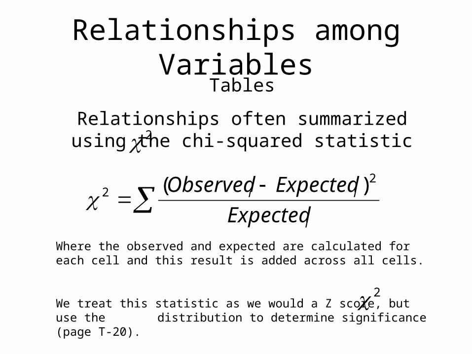
Relationships among VariablesTables
Relationships often summarized using the chi-squared statistic2
i
ii
Expected
ExpectedObserved 22 )(
Where the observed and expected are calculated for each cell and this result is added across all cells.
We treat this statistic as we would a Z score, but use the distribution to determine significance (page T-20).
2

Relationships among Variables
So for the table of income and education we would get the following result:
100
2525252525
625
25
625
25
625
25
62525
)2550(
25
)250(
25
)250(
25
)2550(
)(
2222
22
i
ii
Expected
ExpectedObserved
To find the area in the tail multiply the number of rows -1 by the number of columns-1 or (r-1)*(c-1) to find the df and use that line in table F on page T-20
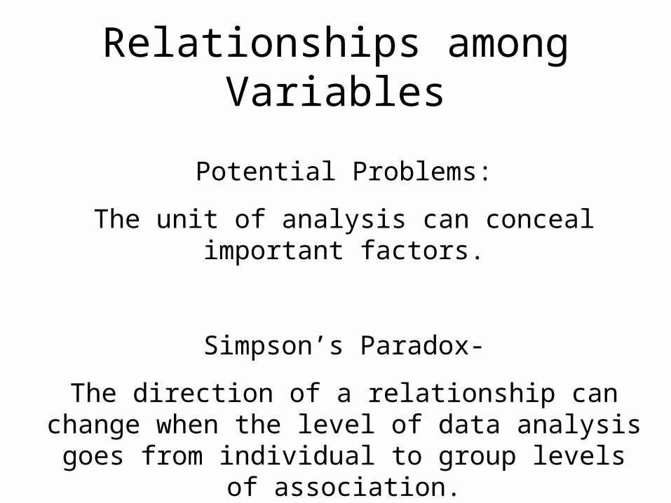
Relationships among Variables
Potential Problems:
The unit of analysis can conceal important factors.
Simpson’s Paradox-
The direction of a relationship can change when the level of data analysis goes from individual to
group levels of association.

Relationships among Variables
University Admissions DecisionsMale Female
Admit 3500 2000
Deny 4500 4000
Total 8000 6000
Acceptance RatesFemale: 2000/6000= 33%Male: 3500/8000= 44%
Is there bias?

Relationships among VariablesUniversity Admissions Decisions by College
Acceptance RatesMale: 50%Female: 50%
Is there bias? What is going on?
Sciences
Male Female
Admit 3000 1000
Deny 3000 1000
Total 6000 2000
MaleFemale
Admit 500 1000
Deny 1500 3000
Total 2000 4000
Acceptance ratesMale: 25%Female: 25%
Humanities

Relationships among Variables
Lurking Variables:
A variable not included in the analysis but that affects the result.
In this case it was that men and women had preferred different majors. Men preferred the
easier to get into major.

Relationships among Variables
Lurking Variable:
A variable not included in the analysis but that affects the result.
X Y

Relationships among Variables
Lurking Variable:
A variable not included in the analysis but that affects the result.
X Y
Z

Relationships among Variables
We can examine the strength of relationships graphically.
Scatter plots-
Show the relationship between two variables when the data are measured on the ordinal, interval, or
ratio scales.

Relationships among Variables
Scatter plot-
(Example here)
Graphs stolen from fiverthirtyeight.com

Relationships among Variables
They can also be used to compare across events.
20082010

Relationships among Variables
We can examine the strength of relationships Statistically.
Measures of Association-
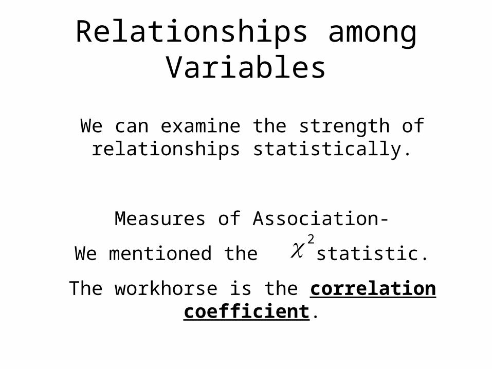
Relationships among Variables
We can examine the strength of relationships statistically.
Measures of Association-
We mentioned the statistic.
The workhorse is the correlation coefficient.
2

Correlation Coefficient

Relationships among VariablesCorrelation Coefficient-
Tells us the linear association between two variables. Ranges from -1.0 (perfect negative
association) to +1.0 a perfect positive association.
Abbreviated as ‘r’
Answers the question:
How far are the points (on average) from the line.

Relationships among Variables-4
-20
24
-4 -2 0 2 4x
Correlation -.7
-4-2
02
4-4 -2 0 2 4
x
Correlation -.5
-4-2
02
4
-4 -2 0 2 4x
Correlation -.3
-4-2
02
4
-4 -2 0 2 4x
Correlation .3
-4-2
02
4
-4 -2 0 2 4x
Correlation .5
-4-2
02
4
-4 -2 0 2 4x
Correlation .7

Relationships among Variables
As a general rule:
r=.7 is a very strong relationship
r=.5 is a strong relationship
r=.3 is a weak relationship
r=0 is no relationship
But it varies depending on how noisy the data are.

Relationships among Variables
Weaknesses:
Does not tell us the magnitude.Example: correlation between education and income =.8. Should you get an MBA?
How can we account for intervening variables?

Regression
Tells us not only the direction but the precise strength of the relationship.
How much increasing one variable changes another variable.

Regression
To clarify this concept we need to be more precise in how we define our variables.
Dependent Variable (Y)-
The thing being explained. Usually the phenomenon we are interested in studying.
Think of this as “the effect”

Regression
Independent Variable (X)-
The thing that affects what we seek to explain.
In overly simplistic terms think of this as
“the cause” or “an influence”

Regression
Regression tells us in precise terms the strength of the relationship between the dependent and
independent variable.
How?
By fitting a line through the data that provides the least squared errors.

Regression
01
0000
200
003
0000
400
00_
_per
ot9
6
0 50000 100000 150000 200000__dole96
OLS picks the line with the smallest sum of squared errors.

Regression
Regression is a process that evaluates the relationship between two variables and selects the
line that minimizes the sum of squared errors around the line.
exy Where:
Y = dependent variable
= intercept
=slope
X= independent variable
e = residual

Regression
The relationship between the independent and dependent variable is summarized by the
regression coefficient which tells us the angle or slope of the line.

Regression
Regression Coefficient (b)-
Tells us how much a one unit change in X causes in Y.
This is called the slope which reflects the angle of the line.

Regression
Intercept-
Tells us what the value of Y is when X is zero. Also called the constant.

Regression
R squared (R2)
Tells us how much of the variation in the dependent variable (Y) our model explained.
Its how well a line fits or describes the data.
Ranges from 0 to 100%.

RegressionWhat is the relationship between the vote for Ross
Perot and Bob Dole in Florida in 1996?
ALWAYS begin by graphing your data.

Regression
01
0000
200
003
0000
400
00_
_per
ot9
6
0 50000 100000 150000 200000__dole96
OLS picks the line with the smallest sum of squared errors.

Regression
regress __perot96 __dole96 Source | SS df MS Number of obs = 67 -------------+------------------------------ F( 1, 65) = 348.69 Model | 4.4790e+09 1 4.4790e+09 Prob > F = 0.0000 Residual | 834933627 65 12845132.7 R-squared = 0.8429 -------------+------------------------------ Adj R-squared = 0.8405 Total | 5.3139e+09 66 80514035.2 Root MSE = 3584 ------------------------------------------------------------------------------ __perot96 | Coef. Std. Err. t P>|t| [95% Conf. Interval] -------------+---------------------------------------------------------------- __dole96 | .1841164 .0098599 18.67 0.000 .1644249 .203808 _cons | 1055.869 548.3668 1.93 0.059 -39.29548 2151.033 ------------------------------------------------------------------------------
Intercept Slope (b) R2

Regression: Interpretationregress __perot96 __dole96 Source | SS df MS Number of obs = 67 -------------+------------------------------ F( 1, 65) = 348.69 Model | 4.4790e+09 1 4.4790e+09 Prob > F = 0.0000 Residual | 834933627 65 12845132.7 R-squared = 0.8429 -------------+------------------------------ Adj R-squared = 0.8405 Total | 5.3139e+09 66 80514035.2 Root MSE = 3584 ------------------------------------------------------------------------------ __perot96 | Coef. Std. Err. t P>|t| [95% Conf. Interval] -------------+---------------------------------------------------------------- __dole96 | .1841164 .0098599 18.67 0.000 .1644249 .203808 _cons | 1055.869 548.3668 1.93 0.059 -39.29548 2151.033 ------------------------------------------------------------------------------
Three main results:1. The slope: for every additional vote Bob Dole received, Perot
got .18 more votes, or for every 100 for Dole, Perot got 18.
2. Where Dole got no votes, we expect Perot to get 1055.
3. The model explains about 84% of the variation in Ross Perot’s vote.

Regression0
100
002
0000
300
004
0000
0 50000 100000 150000 200000__dole96
__perot96 Fitted values
Slope (b)=.184
Intercept =1055
R2=.843

High vs. Low R2
-2-1
01
23
-2 -1 0 1 2x
-3-2
-10
12
-4 -2 0 2 4x
R2=.06R2=.45
Used to compare how well different models explain the data. Higher R2 indicates a better fit.

Regression
Standard Error
To this point, we have assumed that we know the standard deviation of the population.
In practice, we seldom know this, so we estimate it (just as we estimate the population mean). This
estimate is called the standard error.

Regression
We estimate a standard error for the slope and the intercept and use it like we did the standard
deviation—to perform significance tests.

Regression
Here we are conducting a significance test of whether the observed slope and intercept differ
from the null hypothesis.
..
Expected-Observed
EST
This statistic follows a T distribution which accounts for the additional uncertainty that comes from estimating the standard error.

Regression
regress __perot96 __dole96 Source | SS df MS Number of obs = 67 -------------+------------------------------ F( 1, 65) = 348.69 Model | 4.4790e+09 1 4.4790e+09 Prob > F = 0.0000 Residual | 834933627 65 12845132.7 R-squared = 0.8429 -------------+------------------------------ Adj R-squared = 0.8405 Total | 5.3139e+09 66 80514035.2 Root MSE = 3584 ------------------------------------------------------------------------------ __perot96 | Coef. Std. Err. t P>|t| [95% Conf. Interval] -------------+---------------------------------------------------------------- __dole96 | .1841164 .0098599 18.67 0.000 .1644249 .203808 _cons | 1055.869 548.3668 1.93 0.059 -39.29548 2151.033 ------------------------------------------------------------------------------
Intercept Slope (b) R2
Standard Error Standard Error

Regression
We can simply plug the figures in from the Stata output.
67.180099.
0-.184T
This statistic follows a T distribution which accounts for the additional uncertainty that comes from estimating the standard error. (See inside back cover of M&M).
To determine the degrees of freedom subtract the number of variables (2) in the model from the number of observations (67). This is abbreviated as n-k.

Regression
We can simply plug the figures in from the Stata output.
67.180099.
0-.184T
Or, we can use our rule of thumb—if the T statistic is greater than 2 it is significant!

Regression
If we look to the table we see that the p value corresponds to less than .0000 or less than 1 time in 10,000 would we see a result as big as .184 if
the true value were zero.
67.180099.
0-.184T
Stata also reports these p values for us.

Regression: Interpreting the Rest
regress __perot96 __dole96 Source | SS df MS Number of obs = 67 -------------+------------------------------ F( 1, 65) = 348.69 Model | 4.4790e+09 1 4.4790e+09 Prob > F = 0.0000 Residual | 834933627 65 12845132.7 R-squared = 0.8429 -------------+------------------------------ Adj R-squared = 0.8405 Total | 5.3139e+09 66 80514035.2 Root MSE = 3584 ------------------------------------------------------------------------------ __perot96 | Coef. Std. Err. t P>|t| [95% Conf. Interval] -------------+---------------------------------------------------------------- __dole96 | .1841164 .0098599 18.67 0.000 .1644249 .203808 _cons | 1055.869 548.3668 1.93 0.059 -39.29548 2151.033 ------------------------------------------------------------------------------
T Stats P Value
F Statistic- all variables=0

Regression: Residuals
OK—lets interpret this.
reg __clinton96 __perot96 Source | SS df MS Number of obs = 67 -------------+------------------------------ F( 1, 65) = 284.96 Model | 2.3423e+11 1 2.3423e+11 Prob > F = 0.0000 Residual | 5.3429e+10 65 821978256 R-squared = 0.8143 -------------+------------------------------ Adj R-squared = 0.8114 Total | 2.8766e+11 66 4.3585e+09 Root MSE = 28670 ------------------------------------------------------------------------------ __clinton96 | Coef. Std. Err. t P>|t| [95% Conf. Interval] -------------+---------------------------------------------------------------- __perot96 | 6.639231 .3932986 16.88 0.000 5.85376 7.424703 _cons | -9998.995 4509.207 -2.22 0.030 -19004.5 -993.486 ------------------------------------------------------------------------------

Regression: Residuals
Next Up:Residuals
Regression assumptionsMultiple regression.