Post-Quantum Elliptic CurveCryptography

by

Vladimir Soukharev

A thesispresented to the University of Waterloo

in fulfillment of thethesis requirement for the degree of

Doctor of Philosophyin

Computer Science

Waterloo, Ontario, Canada, 2016

c© Vladimir Soukharev 2016

I hereby declare that I am the sole author of this thesis. This is a true copy of the thesis,including any required final revisions, as accepted by my examiners.

I understand that my thesis may be made electronically available to the public.

ii

Abstract

We propose and develop new schemes for post-quantum cryptography based on isoge-nies over elliptic curves. For our first contribution, we show that ordinary elliptic curveshave less than exponential security against quantum computers. These results were usedas the motivation for De Feo, Jao and Plut’s construction of public key cryptosystemsusing supersingular elliptic curve isogenies. We extend their construction and show thatisogenies between supersingular elliptic curves can be used as the underlying hard math-ematical problem for other quantum-resistant schemes. For our second contribution, wepropose an undeniable signature scheme based on elliptic curve isogenies. We prove its se-curity under certain reasonable number-theoretic computational assumptions for which noefficient quantum algorithms are known. This proposal represents only the second knownquantum-resistant undeniable signature scheme, and the first such scheme secure undera number-theoretic complexity assumption. Finally, we also propose a security model forevaluating the security of authenticated encryption schemes in the post-quantum setting.Our model is based on a combination of the classical Bellare-Namprempre security modelfor authenticated encryption together with modifications from Boneh and Zhandry to han-dle message authentication against quantum adversaries. We give a generic constructionbased on Bellare-Namprempre for producing an authenticated encryption protocol from anyquantum-resistant symmetric-key encryption scheme together with any digital signaturescheme or MAC admitting any classical security reduction to a quantum-computationallyhard problem. Using this model, we show how to explicitly construct authenticated en-cryption schemes based on isogenies.

iii

Acknowledgements

I would like to thank my supervisor David Jao.

iv

Dedication

This is dedicated to my wife Viktoriia, my parents Guennadi and Lioubov, and mybrother Pavel.

v

Contents

List of Figures ix

1 Introduction 1

2 Isogenies and Applications to Cryptography 4

2.1 Algebraic Curves . . . . . . . . . . . . . . . . . . . . . . . . . . . . . . . . 4

2.2 Elliptic Curves . . . . . . . . . . . . . . . . . . . . . . . . . . . . . . . . . 10

2.3 Isogenies . . . . . . . . . . . . . . . . . . . . . . . . . . . . . . . . . . . . . 11

2.4 The Endomorphism Ring of Elliptic Curve . . . . . . . . . . . . . . . . . . 15

2.5 Complex Multiplication and Group Action . . . . . . . . . . . . . . . . . . 21

2.6 Application: Stolbunov’s Scheme . . . . . . . . . . . . . . . . . . . . . . . 22

3 Computation of Isogenies Between Ordinary Elliptic Curves 24

3.1 Introduction . . . . . . . . . . . . . . . . . . . . . . . . . . . . . . . . . . . 24

3.2 Isogeny Graphs Under GRH . . . . . . . . . . . . . . . . . . . . . . . . . . 26

3.3 Computing the Action of Cl(O∆) on Ell(O∆) . . . . . . . . . . . . . . . . . 27

3.4 Running Time Analysis . . . . . . . . . . . . . . . . . . . . . . . . . . . . . 28

3.5 A Quantum Algorithm For Constructing Isogenies . . . . . . . . . . . . . . 32

4 Isogeny-Based Quantum-Resistant Key Exchange and Encryption 37

4.1 Introduction . . . . . . . . . . . . . . . . . . . . . . . . . . . . . . . . . . . 37

4.1.1 Ramanujan Graphs . . . . . . . . . . . . . . . . . . . . . . . . . . . 38

4.1.2 Isogeny Graphs . . . . . . . . . . . . . . . . . . . . . . . . . . . . . 39

vi

4.2 Public-Key Cryptosystems Based On Supersingular Curves . . . . . . . . . 39

4.2.1 Zero-Knowledge Proof of Identity . . . . . . . . . . . . . . . . . . . 40

4.2.2 Key Exchange . . . . . . . . . . . . . . . . . . . . . . . . . . . . . . 42

4.2.3 Public-Key Encryption . . . . . . . . . . . . . . . . . . . . . . . . . 43

4.3 Complexity Assumptions . . . . . . . . . . . . . . . . . . . . . . . . . . . . 44

4.3.1 Hardness Of The Underlying Assumptions . . . . . . . . . . . . . . 46

4.4 Security Results . . . . . . . . . . . . . . . . . . . . . . . . . . . . . . . . . 48

5 Isogeny-Based Quantum-Resistant Undeniable Signatures 49

5.1 Introduction . . . . . . . . . . . . . . . . . . . . . . . . . . . . . . . . . . . 49

5.2 Quantum-Resistant Undeniable Signatures From Isogenies . . . . . . . . . 50

5.2.1 Definition . . . . . . . . . . . . . . . . . . . . . . . . . . . . . . . . 50

5.2.2 Protocol . . . . . . . . . . . . . . . . . . . . . . . . . . . . . . . . . 51

5.3 Complexity Assumptions . . . . . . . . . . . . . . . . . . . . . . . . . . . . 54

5.3.1 Hardness Of The Underlying Assumptions . . . . . . . . . . . . . . 55

5.4 Security Proofs . . . . . . . . . . . . . . . . . . . . . . . . . . . . . . . . . 56

5.4.1 Confirmation Protocol . . . . . . . . . . . . . . . . . . . . . . . . . 56

5.4.2 Disavowal Protocol . . . . . . . . . . . . . . . . . . . . . . . . . . . 57

5.4.3 Unforgeability and Invisibility . . . . . . . . . . . . . . . . . . . . . 59

5.5 Parameter Sizes . . . . . . . . . . . . . . . . . . . . . . . . . . . . . . . . . 59

5.6 Conclusion . . . . . . . . . . . . . . . . . . . . . . . . . . . . . . . . . . . . 60

6 Post-Quantum Security Models For Authenticated Encryption 61

6.1 Introduction . . . . . . . . . . . . . . . . . . . . . . . . . . . . . . . . . . . 61

6.2 Security Definitions . . . . . . . . . . . . . . . . . . . . . . . . . . . . . . . 62

6.3 Main Theorem . . . . . . . . . . . . . . . . . . . . . . . . . . . . . . . . . 65

6.4 Quantum-Resistant Strongly Unforgeable Signature Schemes . . . . . . . . 71

6.4.1 Strong Designated Verifier Signatures from Isogenies . . . . . . . . 71

6.4.2 Ring-LWE Signatures . . . . . . . . . . . . . . . . . . . . . . . . . . 72

6.5 Quantum-Resistant Authenticated Encryption . . . . . . . . . . . . . . . . 73

vii

6.6 Isogeny-Based Quantum-Resistant Authenticated Encryption Scheme . . . 74

6.7 Overhead Calculations and Comparisons . . . . . . . . . . . . . . . . . . . 77

6.7.1 Communication Overhead . . . . . . . . . . . . . . . . . . . . . . . 77

6.7.2 Public Key Overhead . . . . . . . . . . . . . . . . . . . . . . . . . . 77

7 Future Work 79

Bibliography 81

viii

List of Figures

2.1 Isogeny volcano . . . . . . . . . . . . . . . . . . . . . . . . . . . . . . . . . 18

2.2 Key agreement protocol by Stolbunov . . . . . . . . . . . . . . . . . . . . . 22

2.3 Public key encryption protocol by Stolbunov . . . . . . . . . . . . . . . . . 23

4.1 Key-exchange protocol using isogenies on supersingular curves. . . . . . . . 43

5.1 Signature generation. . . . . . . . . . . . . . . . . . . . . . . . . . . . . . . 52

5.2 Confirmation protocol. . . . . . . . . . . . . . . . . . . . . . . . . . . . . . 52

5.3 Disavowal protocol. . . . . . . . . . . . . . . . . . . . . . . . . . . . . . . . 54

5.4 Proof of soundness (confirmation) . . . . . . . . . . . . . . . . . . . . . . . 58

5.5 Proof of soundness (disavowal) . . . . . . . . . . . . . . . . . . . . . . . . . 58

5.6 Confirmation (b = 0 case) . . . . . . . . . . . . . . . . . . . . . . . . . . . 58

5.7 Confirmation (b = 1 case) . . . . . . . . . . . . . . . . . . . . . . . . . . . 58

5.8 Disavowal (b = 0 case) . . . . . . . . . . . . . . . . . . . . . . . . . . . . . 58

5.9 Disavowal (b = 1 case) . . . . . . . . . . . . . . . . . . . . . . . . . . . . . 58

6.1 Games G0, G1, and G2. . . . . . . . . . . . . . . . . . . . . . . . . . . . . 68

6.2 Isogenies in Authenticated Encryption Scheme . . . . . . . . . . . . . . . . 76

ix

Chapter 1

Introduction

Elliptic curves, over time, have proven themselves to be a reliable mathematical tools forconstructing cryptographic primitives. The resulting area of cryptography is known as El-liptic Curve Cryptography and remains the object of continued study. The theory of ellipticcurves is well-established and plays an important role in many current areas of research inmathematics. However, in cryptography, applications of elliptic curves to practical cryp-tosystems have so far limited themselves only to the objects, that is, the actual ellipticcurves, rather than the maps between the objects. In contrast, in mathematical research,the study of the maps or morphisms between objects typically demands equal if not moreattention than that of the objects themselves. We believe that it is time to introduce intocryptography the use of maps, or isogenies, between elliptic curves as a direct componentin the design and construction of cryptosystems. Such cryptosystems appear to be a goodcandidate for future post-quantum cryptosystems which are intended to be used in theevent that quantum computers become a reality.

We currently live in an era where the future development of quantum computers is fore-seeable. Many physicists and engineers believe that in about ten to twenty years we willstart seeing quantum computers in practical use. The emergence of quantum computers isan exciting prospect for those who can take advantage of the extra computational capabili-ties that they offer. However, adversaries seeking to attack cryptosystems will also be ableto take advantage of quantum computers. It is well-known that quantum computers canefficiently factor large integers and solve the discrete logarithm problem in finite groupsusing Shor’s algorithm [Sho97]. Most modern-day cryptosystems are based on these twomathematical problems, which are safe against classical adversaries, but will not be safeagainst adversaries with quantum computers. One could in theory use quantum techniquessuch as quantum key distribution to achieve unbreakable encryption that is immune to at-tacks unconditionally, but we do not yet know whether these techniques will scale up tosatisfy future demand. An alternative approach, called Post-Quantum Cryptography, aims

1

to develop cryptosystems for classical computers which would be secure against quantumadversaries.

In recent years, the topic of post-quantum cryptography has been the subject of a greatdeal of interest in the cryptographic research community. Existing families of post-quantumcryptosystems can be divided into five broad subcategories: lattice-based schemes, code-based schemes, hash-based schemes, multivariate polynomials-based schemes, and ellipticcurve-based schemes. Of these, the first four families are firmly established in the literature;the fifth one, which represents our work, is less mainstream at the moment, but attractingincreasing interest. More specifically, our post-quantum elliptic curve cryptosystems arebased on isogenies, which are maps between elliptic curves. Compared to other families, ourapproach has a number of advantages: it is well-suited to key exchange and encryption, andcan achieve signatures and authentication as well with slightly less efficiency. In addition,the relationship between the security parameter and the public parameters to be used inthe system is more straightforward with isogenies than with other families such as lattice-based schemes. We anticipate another benefit to be that existing cryptographic librariesfor elliptic curve arithmetic can be re-used or re-purposed for isogeny-based cryptography,providing a head start in designing high-performance implementations secure against side-channel attacks.

The underlying hard problem for isogeny-based cryptography is: given two isogenoussupersingular elliptic curves, find an isogeny between them. Currently no quantum algo-rithm is known for solving this problem in general in less than exponential time. One ofthe main reasons why this problem seems intractable for quantum computers is that theendomorphism ring for the elliptic curve is non-commutative, which shields the problemagainst attacks like Shor’s algorithm.

In this thesis, we start by providing the necessary mathematical background needed forunderstanding elliptic curves, isogenies, endmorphism rings and complex multiplication.This material can be found in Chapter 2. We also briefly describe Stolbunov’s schemesfrom [Sto10].

In Chapter 3 we describe the computational theory of isogenies. We show how to evalu-ate isogenies between ordinary elliptic curves in subexponential running time (classically).This result appeared previously in my Master’s thesis [Sou10], and portions were also pub-lished in [JS10] and [CJS14], but we include it here because it is necessary backgroundfor later chapters. We then consider the problem of finding isogenies between ordinaryelliptic curves, and show that it can be done in subexponential running time on a quan-tum computer. This result has not previously appeared in any thesis, although it wasalso published in [CJS14]. This chapter shows that ordinary elliptic curves, though widelyused in traditional elliptic curve cryptography, do not provide a good foundation for post-quantum cryptography. For this reason, in the rest of the thesis we consider only the caseof non-ordinary, i.e. supersingular elliptic curves.

2

In Chapter 4, we review the existing constructions of isogeny-based cryptosystems usingsupersingular elliptic curve isogenies. We present the key exchange, public-key encryption,and zero-knowledge proof schemes from [JDF11] and [DFJP14], and discuss the mathemat-ical hard problems on which their security is based. This chapter contains no contributions,but it is necessary background for explaining our contributions.

In Chapter 5, we present a quantum-resistant, isogeny-based undeniable signaturescheme. Of course, as with most asymmetric cryptography, by quantum-resistant we meanthat at present, no quantum algorithm is known, and the research indicates that mostlikely will not be known. We describe our protocol and prove that the scheme satisfies therequired security properties against quantum adversaries. Specifically, we prove that thescheme is unforgeable and invisible and that the confirmation and disavowal protocols arecomplete, sound and zero-knowledge. These results were published in [JS14].

Finally, we present a quantum security model for authenticated encryption based ona combination of existing quantum security models for encryption and signature/MACschemes and existing classical security models for authenticated encryption. We present aquantum analogue of the security model of Bellare and Namprempre [BN08] for quantumadversaries, and show that a quantum-resistant encryption scheme and a quantum-resistantMAC scheme combined using encrypt-then-MAC yields a quantum-resistant authenticatedencryption scheme. These results were published in PQCrypto 2016 [SJS16]. As an appli-cation of our security model, we construct and present an authenticated encryption schemebased on supersingular elliptic curve isogenies. These results are presented in Chapter 6.

3

Chapter 2

Isogenies and Applications toCryptography

In this chapter we give an in-depth treatment of the mathematical and computationaltheory of isogenies. We start with some mathematical background and definitions. Wemention some examples of prior applications of isogenies to cryptography, including count-ing points on elliptic curves over a finite field and the transfer of discrete logarithms. Wealso present Stolbunov’s scheme for encryption using isogenies over ordinary elliptic curves,which represents the first published isogeny-based cryptosystem.

2.1 Algebraic Curves

The goal in this section to briefly present the material needed to be able to define thenotion of isogenies between elliptic curves. The material in this section and the followingtwo sections is contained in [Sil92] (in particular, the first 3 chapters). In many cases,definitions and propositions, theorems, etc. will be used and the proofs omitted. Thereader who is interested in more detail and proofs may refer to that book.

We let K be a perfect field (one whose finite extensions are separable), K a fixedalgebraic closure of K and GK/K the Galois group of K/K.

We first begin with background on affine varieties.

Definition 2.1.1. Affine n-space (over K) is the set of n-tuples

An = An(K) = {P = (x1, . . . , xn) : xi ∈ K}.

Also, the set of K-rational points in An is defined by

An(K) = {P = (x1, . . . , xn) : xi ∈ K}.

4

Note that in this work we will mainly focus on A2 and A3.

Let I ⊂ K[X1, . . . , Xn] be an ideal. Then we associate to I the following subset of An

corresponding to I:VI = {P ∈ An : f(P ) = 0 for all f ∈ I}.

We thus obtain the following definitions:

Definition 2.1.2. An (affine) algebraic set is any set of the form VI . Also, if V is analgebraic set, the ideal of V is given by

I(V ) = {f ∈ K[X1, . . . , Xn] : f(P ) = 0 for all P ∈ V }.

We say that V is defined over K, denoted by V/K, if I(V ) can be generated by polynomialsin K[X1, . . . , Xn]. If V is defined over K, the set of K-rational points of V is the set

V (K) = V ∩ An(K).

We also define I(V/K) = I(V )∩K[X1, . . . , Xn]. If we refer to Hilbert’s basis theorem,we see that all such ideals are finitely generated. In this work we will mainly be concernedwith the case where I(V ) is principal (i.e. generated by one polynomial). Also, note thatif f(X1, . . . , Xn) ∈ K[X1, . . . , Xn] and P ∈ An, then for any σ ∈ GK/K , f(P σ) = f(P )σ.

Definition 2.1.3. V is called an (affine) variety if it is an affine algebraic set such thatI(V ) is a prime ideal in K[X1, . . . , Xn]. If V/K is a variety, then the affine coordinate ringof V/K is defined by

K[V ] =K[X1, . . . , Xn]

I(V/K).

Observe that K[V ] is an integral domain, and its quotient field, denoted by K(V ), is calledthe function field of V/K. (We define K[V ] and K(V ) in a similar manner by replacing Kwith K.)

We need a few more definitions related to the dimension of V .

Definition 2.1.4. Let V be a variety. The dimension of V , denoted by dim(V ), is thetranscendence degree of K(V ) over K.

We will deal primarily with varieties V ⊂ An given by a single non-constant polynomial;in this case dim(V ) = n− 1.

Definition 2.1.5. Let V be a variety, P ∈ V , and f1, . . . , fm ∈ K[X1, . . . , Xn] a set ofgenerators for I(V ). Then we say that V is non-singular (or smooth) at P if the m × nmatrix

(∂fi/∂Xj(P ))1≤i≤m,1≤j≤n

has rank n−dim(V ). If V is non-singular at every point, then we say that V is non-singular(or smooth).

5

When m = 1, a point P ∈ V is a singular point if and only if

∂f/∂X1(P ) = · · · = ∂f/∂Xn(P ) = 0.

We now move to discussing projective varieties. Projective spaces arose through theprocess of adding “points at infinity” to affine spaces.

Definition 2.1.6. Projective n-space (over K), denoted Pn or Pn(K), is the set of all(n+1)-tuples

(x0, . . . , xn) ∈ An+1

such that at least one xi is non-zero, modulo the equivalence relation given by

(x0, . . . , xn) ∼ (y0, . . . , yn)

if there exists a λ ∈ K∗ with xi = λyi for all i. We denote the equivalence class of{(λx0, . . . , λxn)} by [x0, . . . , xn], and we call x0, . . . , xn homogeneous coordinates for thecorresponding point in Pn. As usual, the set of K-rational points in Pn is given by

Pn(K) = {[x0, . . . , xn] ∈ Pn : all xi ∈ K}.

Notice that if P = [x0, . . . , xn] ∈ Pn(K), it does not mean that each xi ∈ K; however,it does mean that choosing some i so that xi 6= 0, we get that each xj/xi ∈ K.

Definition 2.1.7. A polynomial f ∈ K[X0, . . . , Xn] is homogeneous of degree d if

f(λX0, . . . , λXn) = λdf(X0, . . . , Xn)

for all λ ∈ K. An ideal I ⊂ K[X0, . . . , Xn] is homogeneous if it is generated by homoge-neous polynomials.

Given a homogeneous ideal I, we associate a subset of Pn,

VI = {P ∈ Pn : f(P ) = 0 for all homogeneous f ∈ I}.

Definition 2.1.8. A (projective) algebraic set is any set of the form VI . If V is a projectivealgebraic set, the (homogeneous) ideal of V , denoted by I(V ), is the ideal in K[X0, . . . , Xn]generated by

{f ∈ K[X0, . . . , Xn] : f is homogeneous and f(P ) = 0 for all P ∈ V }.

We say that such a V is defined over K, denoted by V/K, if its ideal I(V ) can be generatedby homogeneous polynomials in K[X0, . . . , Xn]. As usual, if V is defined over K, the setof K-rational points of V is the set V (K) = V ∩ Pn(K).

6

Definition 2.1.9. A projective algebraic set V is called a (projective) variety if its homo-geneous ideal I(V ) is a prime ideal in K[X0, . . . , Xn].

Note that Pn contains many copies of An. For each 0 ≤ i ≤ n, we have an inclusion

φi : An → Pn

(y1, . . . , yn) 7→ [y1, y2, . . . , yi−1, 1, yi, . . . , yn].

We define:Ui = {P = [x0, . . . , xn] ∈ Pn : xi 6= 0}

(Notice that U0, . . . , Un cover all of Pn.) Hence, we get a natural bijection

φ−1i : Ui → An

[x0, . . . , xn] 7→ (x0/xi, x1/xi, . . . , xi−1/xi, xi+1/xi, . . . , xn/xi).

Thus, fixing i, we will identify An with the set Ui in Pn via φi. So, given a projectivealgebraic set V with homogeneous ideal I(V ) ⊂ K[X1, . . . , Xn], we will write V ∩ An todenote φ−1

i (V ∩ Ui), which is the affine algebraic set with ideal I(V ∩An) ⊂ K[Y1, . . . , Yn]given by

I(V ∩ An) = {f(Y1, . . . , Yi−1, 1, Yi, . . . , Yn) : f(X0, . . . , Xn) ∈ I(V )}.

This process of replacing f(X0, . . . , Xn) by f(Y1, . . . , Yi−1, 1, Yi, . . . , Yn) is called de-homogenization with respect to Xi. We can also reverse the process—namely, given anon-homogeneous polynomial f(Y1, . . . , Yn) ∈ K[Y1, . . . , Yn], let

f ∗(X0, . . . , Xn) = Xdi f(X0/Xi, X1/Xi, . . . , Xi−1/Xi, Xi+1/Xi, . . . , Xn/Xi)

where d = deg(f) is the smallest integer for which f ∗ is a polynomial. (We call f ∗ thehomogenization of f with respect to Xi.)

Definition 2.1.10. Let V be an affine algebraic set with ideal I(V ), and consider V as asubset of Pn via the map

V ⊂ An φi→ Pn.

The projective closure of V , denoted by V , is the algebraic set whose homogeneous idealI(V ) is generated by

{f ∗(X1, . . . , Xn) : f ∈ I(V )}.

7

In this way, each affine variety can be identified with a unique projective variety. Sincenotationally it is easier to deal with affine coordinates, often, we will write down a non-homogeneous equation for a projective variety V , with the understanding that V is theprojective closure of the given affine variety W . The points V −W are called points atinfinity on V .

Example 2.1.11. Define V to be the projective variety given by the equation

V : Y 2 = X3 + 17.

In this case we really mean the variety in P2 given by homogeneous equation

Y 2Z = X3 + 17Z3.

This variety has one point at infinity, [0, 1, 0] (we obtain it by setting Z = 0).

Certain properties of a projective variety V are defined in terms of the affine (sub)varietyV ∩ An.

Definition 2.1.12. Let V/K be a projective variety. Choose An ⊂ Pn so that V ∩An 6= ∅.The dimension of V is the dimension of V ∩ An. The function field of V , denoted K(V ),is the function field of V ∩ An; similarly for K(V ).

Definition 2.1.13. Let V be a projective variety with P ∈ V . Choose An ⊂ Pn so thatP ∈ An. Then V is non-singular (or smooth) at P if V ∩ An is non-singular at P .

We now move on to algebraic maps between projective varieties, which are the mapsdefined by rational functions.

Definition 2.1.14. Let V1 and V2 ⊂ Pn be projective varieties. A rational map from V1

to V2 is a map of the formφ : V1 → V2

φ = [f0, . . . , fn],

where all fi ∈ K(V1) have the property that for every point P ∈ V1 at which fi’s are alldefined,

φ(P ) = [f0(P ), . . . , fn(P )] ∈ V2.

If V1 and V2 are defined over K, then GK/K acts on φ in the following way:

φσ(P ) = [fσ0 (P ), . . . , fσn (P )].

If there is some λ ∈ K∗ so that λf0, . . . , λfn ∈ K(V1), then φ is said to be defined over K.

8

Definition 2.1.15. A rational map

φ = [f0, . . . , fn] : V1 → V2

is regular (or defined) at P ∈ V1 if there is a function g ∈ K(V1) such that each gfi isregular at P and for some i, (gfi)(P ) 6= 0. If such g exists, we set

φ(P ) = [(gf0)(P ), . . . , (gfn)(P )].

A rational map which is regular at every point is called a morphism.

We now move on to curves, which are projective varieties of dimension 1. We willmostly focus on smooth curves.

Proposition 2.1.16. Let C be a curve, V ⊂ PN a variety, P ∈ C a smooth point, andφ : C → V a rational map. Then φ is regular at P . In particular, if C is smooth, then φis a morphism.

Proof. [Sil92, II.2.1].

Theorem 2.1.17. Let φ : C1 → C2 be a morphism of curves. Then φ is either constant orsurjective.

Proof. [Sil92, II.2.3].

Let C1 and C2 be curves defined over a field K and let φ : C1 → C2 be a non-constantrational map defined over K. The composition with φ induces an injection of functionfields that fixes K:

φ∗ : K(C2)→ K(C1)

φ∗(f) = f ◦ φ.

We are now ready to define the degree of φ.

Definition 2.1.18. Let φ : C1 → C2 be a map of curves defined over K. If φ is constant,we define the degree of φ to be 0. Otherwise, we say that φ is finite, and define its degreeby

deg φ = [K(C1) : φ∗(K(C2))].

We say that φ is separable (inseparable) if the extension K(C1)/φ∗(K(C2)) is separable(inseparable).

It is a known fact that if φ is a non-constant map from curve C1 to curve C2 definedover K, then [K(C1) : φ∗(K(C2))] is finite; hence the definition makes sense.

9

2.2 Elliptic Curves

An elliptic curve is a curve given by a Weierstrass equation over some field F (as shownbelow). An elliptic curve admits an addition operation, which we will define shortly,making the set of points on the curve into an abelian group. We focus on the case wherethe characteristic of the field is different from 2 and 3; the general case may be foundin [Sil92, App. A].

We define the Weierstrass equation to be the locus in P2 of the curve

Y 2Z + a1XY Z + a3Y Z2 = X3 + a2X

2Z + a4XZ2 + a6Z

3,

where a1, . . . , a6 ∈ K. For ease of notation, we use non-homogeneous coordinates to expressthe Weierstrass equation in the following way:

y2 + a1xy + a3y = x3 + a2x2 + a4x+ a6.

We must remember that there is one point at infinity, [0, 1, 0], which we will denote by ∞.If C is the curve represented by the above equation and a1, . . . , a6 ∈ K, then we say thatC is defined over K. If we assume that char(K) 6= 2, 3, then using a change of variable,we can simplify the equation to

y2 = x3 + ax+ b.

There are a few associated values with this curve:

• discriminant ∆ = −16(4a3 + 27b2).

• j-invariant j = −1728(4a)3/∆.

• invariant differential ω = dx/(2y) = dy/(3x2 + b).

The curve represented by the above equation is smooth if and only if ∆ 6= 0.

Definition 2.2.1. Let F be a field such that charF 6= 2, 3. Let a, b ∈ F . An elliptic curveE, defined over the field F , is a set

{(x, y) ∈ F × F : y2 = x3 + ax+ b} ∪ {∞}

.

We will usually denote the elliptic curve by E(F ), E : y2 = x3 + ax + b, or simply byE when the field and equation are known.

As already mentioned, E forms an abelian group under the group law, where the pointat infinity, ∞, is the identity of the group. We define the group law here. Let P =(x1, y1), Q = (x2, y2) ∈ E. Then we define:

10

• P +∞ =∞+ P = P

• −P = (x1,−y1) (assuming P 6=∞)

• P + (−P ) =∞

• P +Q = R = (x3, y3) =(x4

1 − 2ax21 − 8bx1 + a2

4(x31 + ax1 + b)

,(x6

1 + 5ax41 + 20bx3

1 − 5a2x21 − 4abx1 − 8b− a)y1

8(x31 + ax1 + b)2

),

if P = Q and P 6=∞

• P +Q = R = (x3, y3) =(y2

1 − 2y1y2 + y22 − x3

1 + x21x2 + x1x

22 − x3

2

x21 − 2x1x2 + x2

2

,x1y2 − x2y1 + x3y1 − x3y2

x2 − x1

),

if P 6= Q and P,Q 6=∞

When charF is 2 or 3, then the Weierstrass equation simplifies to different forms, withthe discriminant, j-invariant, invariant differential, and the group law modified accordingly.For details see [Sil92, III.1, III.2, A].

2.3 Isogenies

We are now ready to define an isogeny. We give the definition of isogenies and examinesome of their properties. We then present some examples of families of isogenies.

Definition 2.3.1. Let E and E ′ be elliptic curves defined over some field F . An isogenyφ : E → E ′ is an algebraic morphism of the form

φ(x, y) =

(f1(x, y)

g1(x, y),f2(x, y)

g2(x, y)

),

satisfying φ(∞) =∞ (where f ′is and g′is are polynomials in x and y). We say that E1 andE2 are isogenous if there is an isogeny either from E1 to E2 or E2 to E1.

One can show that every isogeny is in fact a group homomorphism [Sil92, III.4.8].

There is only one constant isogeny, namely φ(P ) = ∞ for all P ∈ E1. This constantisogeny is usually denoted by [0], and by convention we let deg[0] = 0. All other isogeniesare non-constant, hence surjective, that is φ(E1) = E2. For all such non-constant isogenies,

11

we define the degree to be the degree as an algebraic map (i.e. [F (E1) : φ∗(F (E2))]); andwe classify the isogeny to be separable (inseparable) if the extension F (E1)/φ∗(F (E2)) isseparable (inseparable).

Let φ : E1 → E2 be a non-constant isogeny. We define kerφ = φ−1(∞). It is knownthat kerφ is a finite subgroup of E1 [Sil92, III.4.9].

Theorem 2.3.2. Let E1, E2 be elliptic curves defined over some field F . Let φ : E1 → E2

be a non-constant separable isogeny. Then # kerφ = deg φ.

Proof. [Sil92, III.4.10(c)].

Proposition 2.3.3. Let E be an elliptic curve over some field F . Let Φ be a finite subgroupof E. Then there exists a unique elliptic curve E ′ (over F ) and a separable isogeny

φ : E → E ′

such thatkerφ = Φ.

Proof. [Sil92, III.4.12].

We now look at a few examples of isogenies.

Example 2.3.4. Scalar multiplication

• Let F be a field of characteristic different from 2 and 3 and E(F ) : y2 = x3 + ax+ bbe an elliptic curve.

• For n ∈ Z, define [n] : E → E by [n](P ) = nP (we usually call this multiplication byn-map). Then [n] is a separable isogeny.

• We can give an explicit algebraic morphism for each such n by using the group lawfor elliptic curves; for instance when n = 2,

[2](x, y) =

(x4 − 2ax2 − 8bx+ a2

4(x3 + ax+ b),

(x6 + 5ax4 + 20bx3 − 5a2x2 − 4abx− 8b− a)y

8(x3 + ax+ b)2

)• Note that the degree of [n] is n2.

• The cardinality of ker([n]) is also n2.

12

• Note that # ker([n]) = deg[n], which agrees with Theorem 2.3.2.

Example 2.3.5. Frobenius map

• Let F = Fq be a finite field of size q (where q is a prime power).

• Let E be an elliptic curve defined over Fq.

• Define π : E → E byπ(x, y) = (xq, yq).

• π is an algebraic map and a group homomorphism, hence an isogeny. In fact, π is aninseparable isogeny.

• Observe that deg(π) = q, but # ker(π) = 1.

• deg(π) 6= # ker(π) because π is inseparable.

Example 2.3.6. Complex multiplication

• Let F be a field such that√−1 ∈ F .

• Let E : y2 = x3 − x be defined over F .

• As usual let i =√−1 ∈ F .

• Defineφ(x, y) = (−x, iy).

• Then φ ◦ φ = [−1].

• This isogeny can be viewed as an extension of scalar multiplication isogenies tocomplex numbers.

Notice that in the definition of isogeny, we stated that elliptic curves are isogenous ifthere exists an isogeny from E1 to E2 or from E2 to E1. In fact, these two conditions areequivalent, as the following result shows.

Theorem 2.3.7. Let E1, E2 be elliptic curves and φ : E1 → E2 be an isogeny defined overfield F . Let m = deg φ. Then there exists a unique isogeny

φ : E2 → E1

that satisfiesφ ◦ φ = [m] (on E1) and φ ◦ φ = [m] (on E2).

13

Proof. [Sil92, III.6.1(a) and III.6.2(a)].

Definition 2.3.8. Let E1, E2 be elliptic curves and φ : E1 → E2 be an isogeny definedover field F . The dual isogeny to φ is the isogeny

φ : E2 → E1

given by 2.3.7. (Note that here we assume that φ 6= [0]. If φ = [0], then we set φ = [0].)

It follows that the relation of being isogenous is an equivalence relation.

We need a few more facts about dual isogenies, which are summarized in the followingtheorem.

Theorem 2.3.9. Let E1, E2, E3 be elliptic curves and let φ : E1 → E2, ϕ : E1 → E2, andψ : E2 → E3 be isogenies defined over field F . Then:

• ψ ◦ φ = φ ◦ ψ.

• φ+ ϕ = φ+ ϕ.

• For all m ∈ Z, [m] = [m] and deg[m] = m2.

• deg φ = deg φ.

• ˆφ = φ.

Proof. [Sil92, III.6.2].

Example 2.3.10. Dual isogenies

• Let F = F109.

• Let E1 : y2 = x3 + 2x + 2 and E2 : y2 = x3 + 34x + 45. An isogeny φ : E1 → E2 (ofdegree 3) is given by

φ(x, y) =

(x3 + 20x2 + 50x+ 6

x2 + 20x+ 100,(x3 + 30x2 + 23x+ 52)y

x3 + 30x2 + 82x+ 19

).

• There exists an isogeny φ : E2 → E1, given by

φ(x, y) =

(x3 + 49x2 + 46x+ 104

9x2 + 5x+ 34,

(x3 + 19x2 + 66x+ 47)y

27x3 + 77x2 + 88x+ 101

),

satisfying φ ◦ φ = [3] and φ ◦ φ = [3].

14

• φ is the dual isogeny of φ and vice-versa.

• Note that this implies that deg(φ ◦ φ) = deg(φ ◦ φ) = 32 = 9.

There is a very useful theorem by Tate which provides us with an efficient method fordetermining whether two curves are isogenous or not.

Theorem 2.3.11. For any two curves E1 and E2 defined over Fq, there exists an isogenyfrom E1 to E2 over Fq if and only if #E1(Fq) = #E2(Fq).

Proof. [Tat66, §3].

Note that using techniques of Schoof in [Sch95], we can compute the number of pointson a given elliptic curve in polynomial time. Hence, we obtain an efficient way to checkwhether two curves are isogenous or not. However, Tate’s theorem does not tell us whatthat isogeny is or how to compute it.

2.4 The Endomorphism Ring of Elliptic Curve

We now define and give some of the properties of the endomorphism ring of an ellipticcurve E. Given elliptic curves E1 and E2 defined over some field F , we set

Hom(E1, E2) = {φ : φ : E1 → E2 is an isogeny over F}.

Definition 2.4.1. Let E be an elliptic curve defined over a field F . Then the endomor-phism ring of E is

End(E) = Hom(E,E).

Notice how in the definition, we have used the term ring. Besides being the set of allisogenies that map from E(F ) to itself, including the constant homomorphism, End(E)is a ring under pointwise addition (i.e. if P ∈ E(F ) and φ1, φ2 ∈ End(E), then (φ1 +φ2)(P ) = φ1(P ) + φ2(P )) with the multiplication operation being composition of isogenies(i.e. (φ1φ2)(P ) = (φ1 ◦ φ2)(P ) = φ1(φ2(P ))).

We now specialize to the case of elliptic curves defined over finite fields.

Theorem 2.4.2. Let E be an elliptic curve defined over a finite field. As a Z-module,dimZ End(E) is equal to either 2 or 4.

Proof. [Sil92, V.3.1].

15

We formulate a definition to distinguish between the two cases.

Definition 2.4.3. An elliptic curve E over a finite field is supersingular if dimZ End(E) =4, and ordinary if dimZ End(E) = 2.

Two isogenous elliptic curves E1 and E2 are either both ordinary, or both supersingular.Thus, there will never be an isogeny between an ordinary and a supersingular elliptic curve.In cryptography, it is traditionally more common to use ordinary curves because they aremore secure for use in discrete logarithm-based schemes. The reason is that Menezes etal. [MOV91] showed that the discrete logarithm problem on a supersingular elliptic curvecan be reduced to a discrete logarithm problem in a finite field, which is easier to solve; thisreduction is referred to as the “MOV reduction.” (The reduction applies to ordinary curvesas well, but it does not speed up the computation of the DLOG in that case.) However,supersingular curves are actually more secure against quantum computers, when we usecryptosystems based on isogenies. These issues will be discussed at length throughout thisthesis.

Before continuing our discussion of endomorphism rings, we need to briefly discuss thetopic of orders in quadratic number fields. This material appears in [Cox89, p. 133].

Definition 2.4.4. An order O in a quadratic field K is a subset O ⊂ K such that:

• O is a subring of K (containing 1).

• O is a finitely generated Z-module.

• O contains a Q-basis of K.

Note that it follows from the definition that O is a free Z-module of rank 2.

When K is a quadratic field, let OK be the ring of integers of K. Then OK is an orderin K. Moreover, if we let O be any order of K, then O ⊂ OK . The order OK is called themaximal order of K.

We can describe these orders more explicitly. Let dK be the discriminant of K and let

wK =dK +

√dK

2.

ThenOK = Z[wK ].

We can also give a more explicit description of an arbitrary order O in K.

16

Lemma 2.4.5. Let O be an order in a quadratic field K of discriminant dK. Then O hasfinite index in OK. Letting c = [OK : O], we have

O = Z + cOK = Z[cwK ],

where wK is defined as above.

Proof. [Cox89, §7].

Note: The index value c in Lemma 2.4.5 is called the conductor of O. Also note thatif we are given an order O of discriminant D, then the discriminant of the maximal orderOK is the largest square-free part of D, i.e. D = c2dK , where dK is the discriminant of OKand c is a conductor. We say that O is an imaginary quadratic order if D < 0, and a realquadratic order otherwise. We denote by O∆ an imaginary quadratic order of discriminant∆.

We now return to the description of the endomorphism ring.

Theorem 2.4.6. Let E be an ordinary elliptic curve defined over the finite field Fq. Then

End(E) ∼= O∆,

where ∆ < 0. That is, the endomorphism ring of E is isomorphic to an imaginary quadraticorder of discriminant ∆.

Proof. [Sil92, V.3.1].

(Note: This ∆ is unrelated to the ∆ that we defined previously as the discriminantof the elliptic curve. From now on, we will use ∆ to refer only to the discriminant of animaginary quadratic order.)

Let E be an elliptic curve defined over Fq, let πq be the Frobenius map, and let t =Trace(πq) be the trace of πq as an element of End(E). The integer t is called the trace ofE. We have a relation t = q + 1−#E(Fq) [Sil92, p. 142] and π2

q − tπq + q = 0.

Let K denote the imaginary quadratic field containing End(E), with maximal orderOK . The field K is called the CM field of E. We write cE for the conductor of End(E)and cπ for the conductor of Z[πq]. It follows from Lemma 2.4.5 and [Cox89, §7] thatEnd(E) ∼= Z + cEOK and ∆ = c2

E∆K , where ∆ (respectively, ∆K) is the discriminant ofthe imaginary quadratic order End(E) (respectively, OK). Furthermore, the characteristicpolynomial x2 − tx + q of πq has discriminant ∆π = t2 − 4q = disc(Z[πq]) = c2

π∆K , withcπ = cE · [End(E) : Z[πq]].

17

Figure 2.1: Isogeny volcano

Following [FM02] and [Gal99], we say that an isogeny φ : E → E ′ of prime degree `defined over Fq is “down” if [End(E) : End(E ′)] = ` (note that this means that End(E ′) ⊂End(E)), “up” if [End(E ′) : End(E)] = ` (note that this means that End(E) ⊂ End(E ′)),and “horizontal” if End(E) = End(E ′). Two curves in an isogeny class are said to “have thesame level” if their endomorphism rings are equal. Within each isogeny class, the propertyof having the same level is an equivalence relation. A horizontal isogeny always goesbetween two curves of the same level; likewise, an up isogeny enlarges the endomorphismring and a down isogeny reduces it. Since there are fewer elliptic curves at higher levelsthan at lower levels, the collection of elliptic curves in an isogeny class visually resemblesa “pyramid” or a “volcano” [FM02], with up isogenies ascending the structure and downisogenies descending. If we restrict to the graph of `-isogenies for a single `, then ingeneral the `-isogeny graph is disconnected, having one `-volcano for each intermediateorder Z[πq] ⊂ O ⊂ OK such that O is maximal at ` (meaning ` - [OK : O]). The “toplevel” of the class consists of curves E with End(E) = OK , and the “bottom level” consistsof curves with End(E) = Z[πq].

The structure of an isogeny volcano is illustrated in Figure 2.1.

We also have the following theorem that states the number of `-isogenies of each type.

Theorem 2.4.7. Let E be an ordinary elliptic curve over Fq, having endomorphism ringEnd(E) of discriminant ∆. Let ` be a prime different from the characteristic of Fq.

• Assume ` - cE. Then there are exactly 1 +(

∆`

)horizontal isogenies φ : E → E ′ of

degree `.

– If ` - cπ, there are no other isogenies E → E ′ of degree ` over Fq.– If ` | cπ, there are `−

(∆`

)down isogenies of degree `.

18

• Assume ` | cE. Then there is one up isogeny E → E ′ of degree `.

– If ` - cπcE

, there are no other isogenies E → E ′ of degree ` over Fq.– If ` | cπ

cE, there are ` down isogenies of degree `.

Proof. [FM02, §2.1] or [Gal99, §11.5].

In light of Theorem 2.4.7, we say that ` is an Elkies prime if(

∆`

)= 1 (implying ` - cE),

or equivalently if and only if E admits exactly two horizontal isogenies of degree `. (Someauthors also allow

(∆`

)= 0, but we do not need this case.)

For the rest of this thesis we will only work with horizontal isogenies over finite fields.That is, unless otherwise stated all definitions and theorems are restricted in scope tohorizontal isogenies.

Definition 2.4.8. Let E1, E2, E3 be elliptic curves over Fq. Let φ : E1 → E2, andφ′ : E1 → E3 be isogenies over Fq. We say that φ and φ′ are isomorphic if there exists anisomorphism η : E2 → E3 such that

η ◦ φ = φ′.

We state a theorem from [Cox89] that we will need.

Theorem 2.4.9. Let L ⊆ C be a lattice. Then for a number α ∈ C \ Z, the followingstatements are equivalent:

(a) αL ⊂ L.

(b) There is an order O in an imaginary quadratic field K such that α ∈ O and L = βIfor some β ∈ C and some proper fractional O-ideal I.

Proof. [Cox89, Theorem 10.14].

Theorem 2.4.10. Let φ : E → E ′ be a (horizontal) isogeny. Then kerφ is a fractionalideal of End(E).

Proof. The proof follows from Theorem 2.4.9. Specifically, let End(E) = OD, α = D+√D

2,

and Φ = kerφ. Observe that the points in Φ lifted to C form the lattice for E ′. Hence,Theorem 2.4.9(a) holds. Therefore Theorem 2.4.9(b) implies that kerφ = βI, where I is a(proper) fractional ideal of some order O, such that End(E) ⊂ O. To show that kerφ isitself a fractional O-ideal, it is enough to show that kerφ ⊂ 1

nEnd(E) for some integer n.

But this relationship clearly holds for n = deg φ.

19

We now show that O ⊂ End(E). We assume the opposite and proceed by contradic-tion. Choose α′ ∈ O \ End(E). In that case, Theorem 2.4.9(b) holds for α′, and thusTheorem 2.4.9(a) implies that α′Φ = Φ, or that O ⊂ End(E ′), which contradicts the factthat End(E ′) = End(E).

Theorem 2.4.11. Let φ : E → E ′ be an isogeny. Then, up to isomorphism, the ideal kerφuniquely determines φ.

Proof. [Sil92, III.4.12].

The above two theorems are very useful because it is usually impractical to expressisogenies algebraically. Rather than expressing the isogeny φ directly, we can represent itusing its kernel kerφ.

We have mostly discussed the ordinary elliptic curves and the structure of their en-domorphism rings. We now need to briefly examine the same for supersingular ellipticcurves. In this case, the structure theory is less well-developed, and in particular there isno known analogue of the “volcano” structure that is present for ordinary curves. Whatis known is that supersingular curves can always be defined over Fp2 , and for every prime` that does not divide p, there exist ` + 1 isogenies (counting multiplicities) of degree `originating from each such supersingular curve.

The structure of the endomorphism ring of a supersingular elliptic curve is that of anorder in a quaternion algebra, which we define here:

Definition 2.4.12. A quaternion algebra over Q is an algebra of the form

Q + Qα + Qβ + Qαβ,

where α2, β2 ∈ Q, α2, β2 < 0, αβ = −βα.

Corollary 2.4.13. The endomorphism ring of an elliptic curve is either Z, an order in aquadratic imaginary field, or an order in a quaternion algebra. In characteristic zero, onlythe first two are possible, and in a finite field, only the latter two are possible.

Proof. [Sil92, III.9.4].

These results show that, since the endomorphism ring of a supersingular elliptic curvehas rank 4, it must be an order in a quaternion algebra. Observe that, unlike the ordinarycase with an imaginary quadratic order, the endomorphism ring of a supersingular ellipticcurve is non-commutative.

20

2.5 Complex Multiplication and Group Action

We know that over the complex numbers, every elliptic curve E is isomorphic to C/Λ forsome lattice Λ = 〈w1, w2〉. In more detail, let Λ ⊂ C be a lattice. Then:

• ℘(z) = 1z2 +

∑w∈Λw 6=0

(1

(z−w)2 − 1w2

)• G4 =

∑w∈Λw 6=0

1w4 , G6 =

∑w∈Λw 6=0

1w6

• φ(z) = (℘(z), ℘′(z)/2)

• E : y2 = x3 − 15G4x− 35G6

As already seen in previous sections, the endomorphism ring of an elliptic curve over afinite field is larger than Z and hence in this case the curve has complex multiplication. Westate here a few important consequences of complex multiplication, but for more detailswe refer to [Wat69], [Lan87] and [Sil94, II].

We first state the following useful theorem:

Theorem 2.5.1. Let E be a given elliptic curve. There is a natural 1-1 correspondencebetween proper ideals a, b ⊂ End(E) and horizontal isogenies φa and φb (up to isomorphismof isogenies) between the corresponding curves. As a result, we also have:

• φab = φa ◦ φb.

• deg φa equals the norm of a.

Proof. For the case when End(E) is a maximal order see [Sil94, II.1.2]. For more generalcases see [Lan87].

This theorem shows that using ideals to represent isogenies does not affect the mainarithmetic properties of isogenies.

We need to define the following set:

Definition 2.5.2. The set of isomorphism classes of elliptic curves E/Fq with End(E) =OK is denoted Ellp,n(OK), where n = #E.

Thus, let us denote by φb : E → Eb the isogeny corresponding to an ideal b (keepingin mind that φb is only defined up to isomorphism of Eb). Principal ideals correspond toendomorphisms, so any other ideal equivalent to b in the ideal class group Cl(O∆) of O∆

21

yields the same codomain curve Eb, up to isomorphism [Wat69, Thm. 3.11]. Hence oneobtains a well-defined group action ∗ : Cl(O∆)×Ellq,n(O∆)→ Ellq,n(O∆) taking [b] ∗ j(E)to j(Eb), where [b] denotes the ideal class of b. This group action, which we call the complexmultiplication operator, is free and transitive [Wat69, Thm. 4.5], and thus Ellq,n(O∆) formsa principal homogeneous space over Cl(O∆).

2.6 Application: Stolbunov’s Scheme

In this section we briefly present two examples by Stolbunov [Sto10] of cryptosystems basedon isogenies between ordinary elliptic curves. One scheme is for key exchange and the otheris for public key encryption.

For the following two schemes, we let x be an ordinary elliptic curve over some finitefield. We let G be a set of isogenies in End(x), but in practice should be all of End(x).Finally we let H = {Hk : k ∈ K} be a set of secure hash functions indexed by a finite setK. (The family H is needed to be able to prove the security of the scheme.)

Figure 2.2: Key agreement protocol by Stolbunov

We also give the statements of the security proofs from Stolbunov’s paper.

Theorem 2.6.1. The key exchange protocol in figure 2.2 is session-key (SK) secure in theauthenticated-links adversarial model (AM).

Proof. [Sto10, Theorem 1].

Theorem 2.6.2. The public-key encryption protocol in figure 2.3 is secure in the sense ofIND-CPA.

22

Figure 2.3: Public key encryption protocol by Stolbunov

Proof. [Sto10, Theorem 2].

These security results only hold if the underlying mathematical problem of computingisogenies between ordinary elliptic curves is hard. Although this problem seems to be hardfor classical computers, we show in the next chapter that it is easier to solve on a quantumcomputer.

23

Chapter 3

Computation of Isogenies BetweenOrdinary Elliptic Curves

3.1 Introduction

This chapter consists of material from our published article in the Journal of MathematicalCryptology [CJS14], co-authored with Andrew Childs and my supervisor David Jao. Some(but not all) of this material also appeared in [Sou10] (my Master’s Thesis). The lastsection of this chapter has not previously appeared in any thesis, and serves to motivatethe use of supersingular elliptic curve isogenies in post-quantum cryptography.

We address two notions in this chapter - evaluating isogenies and computing or con-structing isogenies. Evaluating isogenies means that whenever we are given an ellipticcurve and an isogeny mapping from it, we wish to evaluate that isogeny. Computing orconstructing isogenies means that whenever we are given to isogenous elliptic curves, wewish to find the isogeny between them.

In this chapter we present and describe in details our algorithm for evaluating largeprime degree isogenies, having subexponential running time in the size of the magnitude ofthe discriminant of the endomorphism ring of the elliptic curve and polynomial in the sizeof the degree of the isogeny. The proofs of correctness and the running-time analysis relyon only one standard assumption, namely the Generalized Riemann Hypothesis (GRH).

Our first objective is to evaluate an isogeny of large degree in subexponential time,given a compact representation. Specifically, we wish to evaluate the unique horizontalnormalized [BCL08] isogeny on a given elliptic curve E/Fq whose kernel ideal in End(E)is given as L = (`, c + dπq), at a given point P ∈ E(Fqn), where ` is an Elkies prime, πqdenotes the Frobenius map on E, and c and d are rational numbers specifying the ideal L

24

and hence the isogeny. As in [BCL08], we must also impose the additional restriction that` - [End(E) : Z[πq]]; for Elkies primes, an equivalent restriction is that ` - [OK : Z[πq]], butwe retain the original formulation for consistency with [BCL08].

In practice, one is typically given ` instead of L, but since it is easy to calculate the list of(at most two) possible primes L lying over ` (cf. [BV07]), these two interpretations are for allpractical purposes equivalent, and we switch freely between them when convenient. When` is small, one can use modular polynomial based techniques [BCL08, §3.1], which haverunning time O(`3 log(`)4+ε) [Eng09]. However, for isogeny degrees of cryptographic size(e.g. 2160), this approach is impractical. The Broker-Charles-Lauter algorithm sidestepsthis problem, by using an alternative factorization of L. However, the running time ofBroker-Charles-Lauter is polynomial in |∆| (where ∆ is the discriminant of End(E)), andtherefore even this method only works for small values of |∆|. In this chapter we present amodified version of the Broker-Charles-Lauter algorithm which is suitable for large valuesof |∆|.

We give an overview of our approach. In order to handle large values of |∆|, there aretwo main problems to overcome. One problem is that we need a fast way to produce afactorization

L = Ie11 Ie22 · · · I

ekk · (α) (3.1)

as in lines 2 and 3 of the BCL algorithm (Algorithm 4.1 in [BCL08]). The other problemis that the exponents ei in Equation (3.1) need to be kept small, since the running times oflines 3 and 4 of Algorithm 4.1 in [BCL08] are proportional to

∑i |ei|Norm(Ii)

2. The firstproblem, that of finding a factorization of L, can be solved in subexponential time usingthe index calculus algorithm of Hafner and McCurley [HM89] (see also [BV07, Chapter11]). To resolve the second problem, we turn to the following idea of Galbraith, Hess, andSmart [GHS02], and recently further refined by Bisson and Sutherland [BS11]. The ideais that, in the process of sieving for smooth norms, one can arbitrarily restrict the inputexponent vectors to sparse vectors (e1, e2, ..., ek) such that

∑i |ei|N(Ii)

2 is kept small. Thedetails of this approach can be found in [JS10].

We present a variant of the algorithm. Our variant improves on the above describedalgorithm in the sense that we remove all heuristic assumptions except GRH. In practicethe new algorithm is slower, although asymptotically it has the same running time asbefore, with the same constants in the exponents.

Finally, in this chapter, we give a subexponential-time quantum algorithm for construct-ing a nonzero isogeny between two given elliptic curves (of the type arising in the afore-mentioned cryptosystems). We show that the running time of our algorithm is bounded

above by Lq(12,√

32

) under (only) the Generalized Riemann Hypothesis (GRH), where

LN(α, c) := exp[(c+ o(1))(lnN)α(ln lnN)1−α].

25

This result raises serious questions about the viability of isogeny-based cryptosystems overordinary curves in the context of quantum computers.

3.2 Isogeny Graphs Under GRH

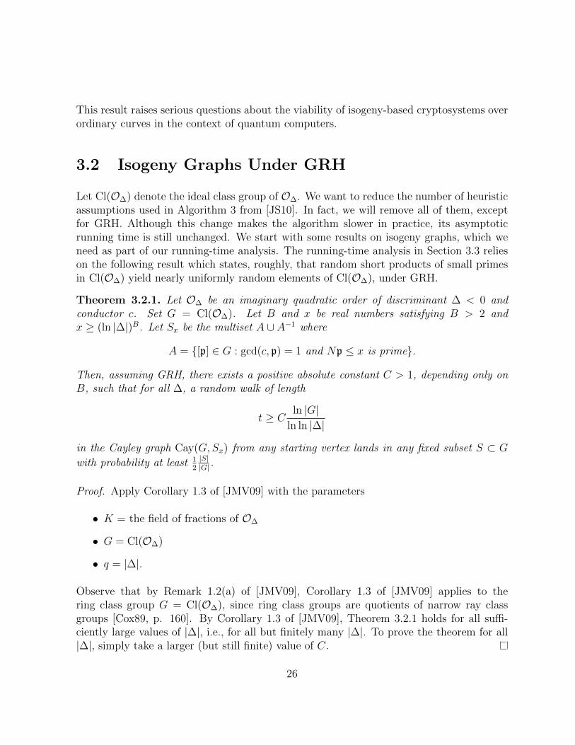
Let Cl(O∆) denote the ideal class group of O∆. We want to reduce the number of heuristicassumptions used in Algorithm 3 from [JS10]. In fact, we will remove all of them, exceptfor GRH. Although this change makes the algorithm slower in practice, its asymptoticrunning time is still unchanged. We start with some results on isogeny graphs, which weneed as part of our running-time analysis. The running-time analysis in Section 3.3 relieson the following result which states, roughly, that random short products of small primesin Cl(O∆) yield nearly uniformly random elements of Cl(O∆), under GRH.

Theorem 3.2.1. Let O∆ be an imaginary quadratic order of discriminant ∆ < 0 andconductor c. Set G = Cl(O∆). Let B and x be real numbers satisfying B > 2 andx ≥ (ln |∆|)B. Let Sx be the multiset A ∪ A−1 where

A = {[p] ∈ G : gcd(c, p) = 1 and Np ≤ x is prime}.

Then, assuming GRH, there exists a positive absolute constant C > 1, depending only onB, such that for all ∆, a random walk of length

t ≥ Cln |G|

ln ln |∆|

in the Cayley graph Cay(G,Sx) from any starting vertex lands in any fixed subset S ⊂ G

with probability at least 12|S||G| .

Proof. Apply Corollary 1.3 of [JMV09] with the parameters

• K = the field of fractions of O∆

• G = Cl(O∆)

• q = |∆|.

Observe that by Remark 1.2(a) of [JMV09], Corollary 1.3 of [JMV09] applies to thering class group G = Cl(O∆), since ring class groups are quotients of narrow ray classgroups [Cox89, p. 160]. By Corollary 1.3 of [JMV09], Theorem 3.2.1 holds for all suffi-ciently large values of |∆|, i.e., for all but finitely many |∆|. To prove the theorem for all|∆|, simply take a larger (but still finite) value of C.

26

Corollary 3.2.2. For any fixed integer m, Theorem 3.2.1 holds even if the definition ofthe set A is changed to

A = {[p] ∈ G : gcd(m∆, p) = 1 and Np ≤ x is prime}.

Proof. The alternative definition of A differs from the original definition by at most O(ln q)primes. As stated in [JMV09, p. 1497], such a change does not affect the conclusion of thetheorem.

3.3 Computing the Action of Cl(O∆) on Ell(O∆)

In this section, we describe a new algorithm to evaluate the horizontal isogeny correspond-ing to a given kernel. In contrast with the Algorithm 4 in [JS10], this algorithm relieson no heuristic assumptions other than GRH. In terms of performance, this algorithm isslightly slower, although its running time is still L|∆|(

12,√

32

). The algorithm takes as inputa discriminant ∆, an elliptic curve E, a point P , and a kernel ideal L, and outputs φ(P ),where φ : E → E ′ is the normalized horizontal isogeny corresponding to L.

In this section, we describe the steps in our algorithm. In Section 3.4 we show that,under GRH, our algorithm has a running time of Lq(

12,√

32

), which is subexponential in theinput size. We stress that although similar algorithms have appeared in several previousworks, our algorithm is the first to achieve provably subexponential running time withoutappealing to any conditional hypotheses other than GRH.

We present our algorithm in several stages.

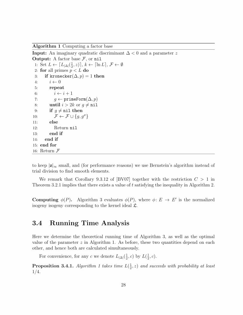
Computing a factor base. Algorithm 1 computes a factor base for Cl(O∆) consistingof all split primes up to L|∆|(

12, z). The optimal value of the parameter z is determined

in Section 3.4. The algorithm is based on, and indeed almost identical to, Algorithm 11.1in [BV07]. The subroutine primeForm [BV07, §3.4] calculates a quadratic form correspond-ing to a prime ideal of norm p, and the subroutine kronecker [BV07, §3.4.3] calculates theKronecker symbol. The map σ denotes complex conjugation.

Computing a relation. Given a factor base F = {p1, . . . , pf} and an ideal class [b] ∈Cl(O∆), Algorithm 2 produces a relation vector z = (z1, . . . , zf ) ∈ Zf for [b] satisfying[b] = Fz := pz11 · · · p

zff , with the additional property that the L∞-norm |z|∞ of z is less

than O(ln |∆|) for some absolute implied constant (cf. Proposition 3.4.5). It is similar toAlgorithm 11.2 in [BV07], except that we impose a constraint on |v|∞ in line 1 in order

27

Algorithm 1 Computing a factor base

Input: An imaginary quadratic discriminant ∆ < 0 and a parameter zOutput: A factor base F , or nil1: Set L← dL|∆|(1

2, z)e, k ← dlnLe, F ← ∅

2: for all primes p < L do3: if kronecker(∆, p) = 1 then4: i← 05: repeat6: i← i+ 17: g ← primeForm(∆, p)8: until i > 2k or g 6= nil

9: if g 6= nil then10: F ← F ∪ {g, gσ}11: else12: Return nil

13: end if14: end if15: end for16: Return F

to keep |z|∞ small, and (for performance reasons) we use Bernstein’s algorithm instead oftrial division to find smooth elements.

We remark that Corollary 9.3.12 of [BV07] together with the restriction C > 1 inTheorem 3.2.1 implies that there exists a value of t satisfying the inequality in Algorithm 2.

Computing φ(P ). Algorithm 3 evaluates φ(P ), where φ : E → E ′ is the normalizedisogeny isogeny corresponding to the kernel ideal L.

3.4 Running Time Analysis

Here we determine the theoretical running time of Algorithm 3, as well as the optimalvalue of the parameter z in Algorithm 1. As before, these two quantities depend on eachother, and hence both are calculated simultaneously.

For convenience, for any c we denote L|∆|(12, c) by L(1

2, c).

Proposition 3.4.1. Algorithm 1 takes time L(12, z) and succeeds with probability at least

1/4.

28

Algorithm 2 Computing a relation

Input: A discriminant ∆ < 0, a parameter z, a factor base F of size f , an ideal class[b] ∈ Cl(O∆), and an integer t satisfying C ln |Cl(O∆)|

ln ln |∆| ≤ t ≤ C ln |∆| where C is the

constant of Theorem 3.2.1/Corollary 3.2.2Output: A relation vector z ∈ Zf such that [b] = [Fz], or nil1: Set S ← ∅, P ← {N(p) : p ∈ F}2: Set `← L|∆|(

12, 1

4z)

3: for i = 0 to ` do4: Select v ∈ Zf0..|∆|−1 uniformly at random subject to the condition that |v|∞ = t

5: Calculate the reduced ideal av in the ideal class [b] · [Fv]6: Set S ← S ∪N(av)7: end for8: Using Bernstein’s algorithm [Ber], find a P-smooth element N(av) ∈ S (if there exists

one), or else return nil

9: Find the prime factorization of the integer N(av)10: Using Seysen’s algorithm [Sey87, Thm. 3.1] on the prime factorization of N(av), factor

the ideal av over F to obtain av = Fa for some a ∈ Zf11: Return z = a− v

Proof. Since Algorithm 1 is identical to Algorithm 11.1 in [BV07], the proposition followsfrom Lemmas 11.3.1 and 11.3.2 of [BV07].

Proposition 3.4.2. The running time of Algorithm 2 is at most L(12, z) + L(1

2, 1

4z), as-

suming GRH.

Proof. Line 1 of the algorithm requires L(12, z) norm computations. Line 2 is negligi-

ble. Line 5 requires C ln |∆| multiplications in the class group, each of which requiresO((ln |∆|)1+ε) bit operations [Sch91]. Hence the for loop in lines 3–7 has running timeL(1

2, 1

4z). Bernstein’s algorithm [Ber] in line 8 has a running time of b(log2 b)

2+ε whereb = L(1

2, z) + L(1

2, 1

4z) is the combined size of S and P . Finding the prime factorization

in line 9 costs L(12, z) using trial division, and Seysen’s algorithm [Sey87, Thm. 3.1] in line

10 has negligible cost under ERH (and hence GRH). Accordingly, we find that the runningtime is

L(12, z) +O((ln |∆|)2+ε) + L(1

2, 1

4z) + b(log2 b)

2+ε + L(12, z) = L(1

2, z) + L(1

2, 1

4z),

as desired.

Proposition 3.4.3. Under GRH, the probability that a single iteration of the for loop ofAlgorithm 2 produces an F-smooth ideal av is at least L(1

2,− 1

4z).

29

Algorithm 3 Evaluating prime degree isogenies

Input: A discriminant ∆ < 0, an elliptic curve E/Fq with End(E) = O∆, a point P ∈E(Fq) such that [End(E) : Z[Frobq]] and #E(Fq) are coprime, and an End(E)-idealL = (`, c + dFrobq) of prime norm ` 6= char(Fq) not dividing the index [End(E) :Z[Frobq]].

Output: The unique elliptic curve E ′ admitting a normalized isogeny φ : E → E ′ withkernel E[L], and the x-coordinate of φ(P ) for ∆ 6= −3,−4 or the square (resp. cube)of the x-coordinate otherwise.

1: Using Algorithm 1, compute a factor base; discard any primes dividing qn to obtain anew factor base F = {p1, p2, . . . , pf}

2: Using Algorithm 2 with any valid choice of t, compute a relation z ∈ Zf such that[L] = [Fz] = [pz11 pz22 · · · p

zff ]

3: Compute a sequence of isogenies (φ1, . . . , φs) such that the composition φc : E → Ecof the sequence has kernel E[pz11 pz22 · · · p

zff ], using the method of [BCL08, §3]

4: Using Cornacchia’s algorithm, find a generator α ∈ O∆ of the fractional idealL/(pz11 pz22 · · · p

zff )

5: Evaluate φc(P ) ∈ Ec(Fq)6: Write α = (u + v Frobq)/z, compute the isomorphism η : Ec

∼→ E ′ with η∗(ωE′) =(u/z)ωEc , and compute Q = η(φc(P ))

7: Compute z−1 mod #E(Fqn) and R = (z−1(u+ v Frobq))(Q)8: Put r = x(R)|O

∗∆|/2 and return (E ′, r)

Proof. We adopt the notation used in Theorem 3.2.1 and Corollary 3.2.2. Apply Corol-lary 3.2.2 with the values m = qn, B = 3, and x = f = L(1

2, z)� (ln |∆|)B. The ideal class

[b] · [Fv] is equal to the ideal class obtained by taking the walk of length t in the Cayleygraph Cay(G,Sx), having initial vertex [b], and whose edges correspond to the nonzerocoordinates of the vector v. Hence a random choice of vector v under the constraintsof Algorithm 2 yields the same probability distribution as a random walk in Cay(G,Sx)starting from [b].

Let S be the set of reduced ideals in G with L(12, z)-smooth norm. By [BV07, Lemma

11.4.4], |S| ≥√|∆|L(1

2,− 1

4z). Hence, by Corollary 3.2.2, the probability that av lies in S

is at least1

2

|S||G|

=1

2·√|∆||G|

· L(12,− 1

4z).

Finally, Theorem 9.3.11 of [BV07] states that

√|∆||G| ≥

1ln |∆| . Hence the probability that av

is F -smooth is at least1

2· 1

ln |∆|· L(1

2,− 1

4z) = L(1

2,− 1

4z).

30

The result follows.

Corollary 3.4.4. Under GRH, the probability that Algorithm 2 succeeds is at least 1− 1e.

Proof. Algorithm 2 loops through ` = L(12, 1

4z) vectors v, and by Proposition 3.4.3, each

such choice of v has an independent 1/` chance of producing a smooth ideal av. Thereforethe probability of success is at least

1−(

1− 1

`

)`> 1− 1

e,

as desired.

The following proposition shows that the relation vector z produced by Algorithm 2 isguaranteed to have small coefficients.

Proposition 3.4.5. Any vector z output by Algorithm 2 satisfies |z|∞ < (C + 1) ln |∆|.

Proof. Since z = a− v, we have |z|∞ ≤ |a|∞+ |v|∞. But |v|∞ ≤ C ln |∆| by construction,and the norm of av is less than

√|∆|/3 [BV07, Prop. 9.1.7], which implies

|a|∞ < log2

√|∆|/3 < log2

√|∆| < ln |∆|.

This completes the proof.

Finally, we analyze the running time of Algorithm 3.

Theorem 3.4.6. Under GRH, Algorithm 3 succeeds with probability at least 14(1− 1

e) and

runs in time at most

L(12, 1

4z) + max{L(1

2, 3z), L(1

2, z)(ln q)3+ε}.

Proof. We have shown that Algorithm 1 has running time L(12, z) and success probability

at least 1/4, and Algorithm 2 has running time L(12, z)+L(1

2, 1

4z) and success probability at

least 1− 1e. Assuming that both these algorithms succeed, the computation of the individual

isogenies φi in line 3 of Algorithm 3 proceeds in one of two ways, depending on whether thecharacteristic of Fq is large [BCL08, §3.1] or small [BCL08, §3.2]. The large characteristicalgorithm fails when the characteristic is small, whereas the small characteristic algorithmsucceeds in all situations, but is slightly slower in large characteristic. For simplicity, weconsider only the more general algorithm.

The general algorithm proceeds in two steps. In the first step, we compute the kernelpolynomial of the isogeny. The time to perform one such calculation is

31

O((`(ln q) max(`, ln q)2)1+ε) in all cases ([LS08, Thm. 1] for characteristic ≥ 5 and [DF10,Thm. 1] for characteristic 2 or 3). In the second step, we evaluate the isogeny using Velu’sformulae [Vel71]. This second step has a running time of O(`2+ε(ln q)1+ε) [IJ10, p. 214].Hence the running time of line 3 is at most

|z|∞(O((`(ln q) max(`, ln q)2)1+ε) +O(`2+ε(ln q)1+ε)).

By Proposition 3.4.5, this expression is at most

(C + 1)(ln |∆|)(max{L(12, 3z), L(1

2, z)(ln q)3+ε}+ L(1

2, 2z)(ln q)1+ε)

= max{L(12, 3z), L(1

2, z)(ln q)3+ε}.

Since the running time of all other lines in Algorithm 3 is bounded by that of line 3, thetheorem follows.

Corollary 3.4.7. Under GRH, Algorithm 3 has a worst-case running time of at mostLq(

12,√

32

).

Proof. Using the inequality |∆| ≤ 4q, we may rewrite Theorem 3.4.6 in terms of q. Weobtain

L(12, 1

4z) + max{L(1

2, 3z), L(1

2, z)(ln q)3+ε} ≤ Lq(

12, 1

4z+ 3z).

The optimal choice of z = 12√

3yields the running time bound of Lq(

12,√

32

).

3.5 A Quantum Algorithm For Constructing Isoge-

nies

We now move on to the quantum approach to solving the problem of finding and evaluatingthe isogeny between two given ordinary elliptic curves. Note that this problem is harderthan the previous one that we looked at. In fact, it is believed to be exponential for aclassical computer. However, quantum computers are able to solve more classes of problemsand we take advantage of that. Since evaluating the isogeny can be done subexponentially,we are left to show that finding the isogeny itself can also be done subexponentially, usinga quantum computer.

Our quantum algorithm for constructing isogenies uses a simple reduction to the abelianhidden shift problem. This problem is defined as follows. Let A be a known finite abeliangroup (with the group operation written multiplicatively) and let f0, f1 : A→ S be black-box functions, where S is a known finite set. We say that f0, f1 hide a shift s ∈ A iff0 is injective and f1(x) = f0(xs) (i.e., f1 is a shifted version of f0). The goal of the

32

hidden shift problem is to determine s using queries to such black-box functions. Notethat this problem is equivalent to the hidden subgroup problem in the A-dihedral group,the nonabelian group Ao Z2 where Z2 acts on A by inversion.

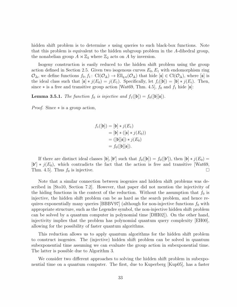
Isogeny construction is easily reduced to the hidden shift problem using the groupaction defined in Section 2.5. Given two isogenous curves E0, E1 with endomorphism ringO∆, we define functions f0, f1 : Cl(O∆) → Ellq,n(O∆) that hide [s] ∈ Cl(O∆), where [s] isthe ideal class such that [s] ∗ j(E0) = j(E1). Specifically, let fi([b]) = [b] ∗ j(Ei). Then,since ∗ is a free and transitive group action [Wat69, Thm. 4.5], f0 and f1 hide [s]:

Lemma 3.5.1. The function f0 is injective and f1([b]) = f0([b][s]).

Proof. Since ∗ is a group action,

f1([b]) = [b] ∗ j(E1)

= [b] ∗ ([s] ∗ j(E0))

= ([b][s]) ∗ j(E0)

= f0([b][s]).

If there are distinct ideal classes [b], [b′] such that f0([b]) = f0([b′]), then [b] ∗ j(E0) =[b′] ∗ j(E0), which contradicts the fact that the action is free and transitive [Wat69,Thm. 4.5]. Thus f0 is injective.

Note that a similar connection between isogenies and hidden shift problems was de-scribed in [Sto10, Section 7.2]. However, that paper did not mention the injectivity ofthe hiding functions in the context of the reduction. Without the assumption that f0 isinjective, the hidden shift problem can be as hard as the search problem, and hence re-quires exponentially many queries [BBBV97] (although for non-injective functions f0 withappropriate structure, such as the Legendre symbol, the non-injective hidden shift problemcan be solved by a quantum computer in polynomial time [DHI02]). On the other hand,injectivity implies that the problem has polynomial quantum query complexity [EH00],allowing for the possibility of faster quantum algorithms.

This reduction allows us to apply quantum algorithms for the hidden shift problemto construct isogenies. The (injective) hidden shift problem can be solved in quantumsubexponential time assuming we can evaluate the group action in subexponential time.The latter is possible due to Algorithm 3.

We consider two different approaches to solving the hidden shift problem in subexpo-nential time on a quantum computer. The first, due to Kuperberg [Kup05], has a faster

33

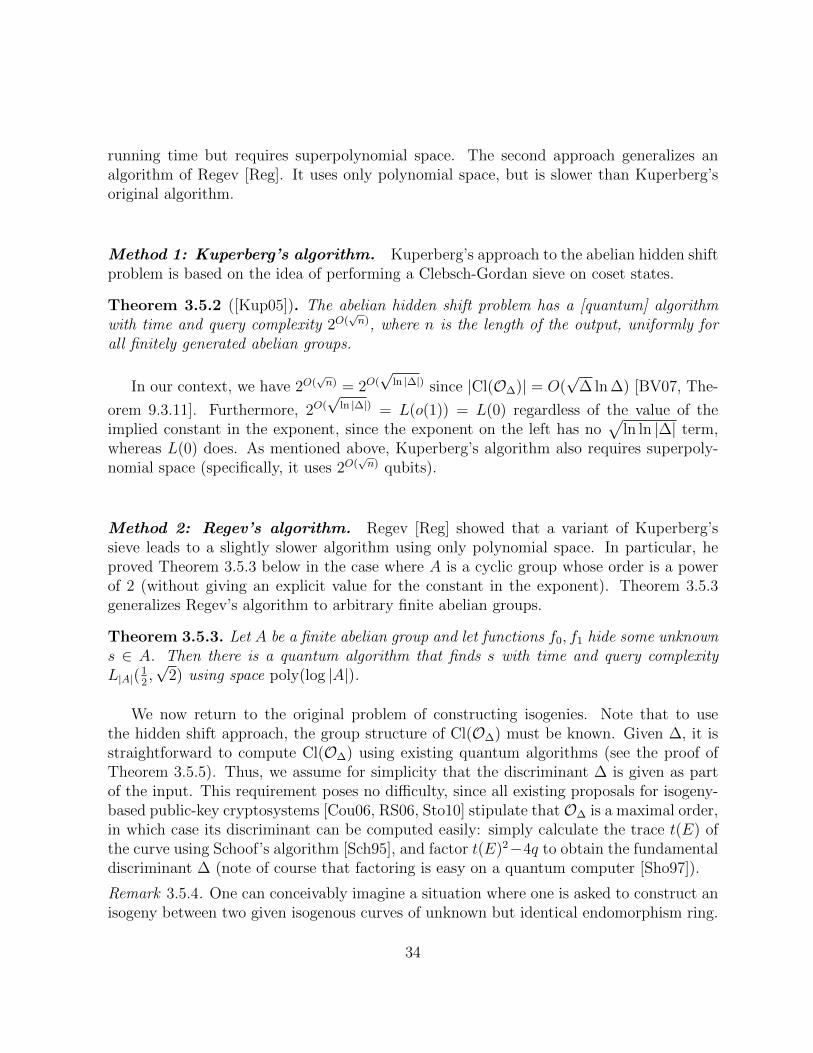
running time but requires superpolynomial space. The second approach generalizes analgorithm of Regev [Reg]. It uses only polynomial space, but is slower than Kuperberg’soriginal algorithm.

Method 1: Kuperberg’s algorithm. Kuperberg’s approach to the abelian hidden shiftproblem is based on the idea of performing a Clebsch-Gordan sieve on coset states.

Theorem 3.5.2 ([Kup05]). The abelian hidden shift problem has a [quantum] algorithmwith time and query complexity 2O(

√n), where n is the length of the output, uniformly for

all finitely generated abelian groups.

In our context, we have 2O(√n) = 2O(

√ln |∆|) since |Cl(O∆)| = O(

√∆ ln ∆) [BV07, The-

orem 9.3.11]. Furthermore, 2O(√

ln |∆|) = L(o(1)) = L(0) regardless of the value of theimplied constant in the exponent, since the exponent on the left has no

√ln ln |∆| term,

whereas L(0) does. As mentioned above, Kuperberg’s algorithm also requires superpoly-nomial space (specifically, it uses 2O(

√n) qubits).

Method 2: Regev’s algorithm. Regev [Reg] showed that a variant of Kuperberg’ssieve leads to a slightly slower algorithm using only polynomial space. In particular, heproved Theorem 3.5.3 below in the case where A is a cyclic group whose order is a powerof 2 (without giving an explicit value for the constant in the exponent). Theorem 3.5.3generalizes Regev’s algorithm to arbitrary finite abelian groups.

Theorem 3.5.3. Let A be a finite abelian group and let functions f0, f1 hide some unknowns ∈ A. Then there is a quantum algorithm that finds s with time and query complexityL|A|(

12,√

2) using space poly(log |A|).

We now return to the original problem of constructing isogenies. Note that to usethe hidden shift approach, the group structure of Cl(O∆) must be known. Given ∆, it isstraightforward to compute Cl(O∆) using existing quantum algorithms (see the proof ofTheorem 3.5.5). Thus, we assume for simplicity that the discriminant ∆ is given as partof the input. This requirement poses no difficulty, since all existing proposals for isogeny-based public-key cryptosystems [Cou06, RS06, Sto10] stipulate thatO∆ is a maximal order,in which case its discriminant can be computed easily: simply calculate the trace t(E) ofthe curve using Schoof’s algorithm [Sch95], and factor t(E)2−4q to obtain the fundamentaldiscriminant ∆ (note of course that factoring is easy on a quantum computer [Sho97]).

Remark 3.5.4. One can conceivably imagine a situation where one is asked to construct anisogeny between two given isogenous curves of unknown but identical endomorphism ring.

34

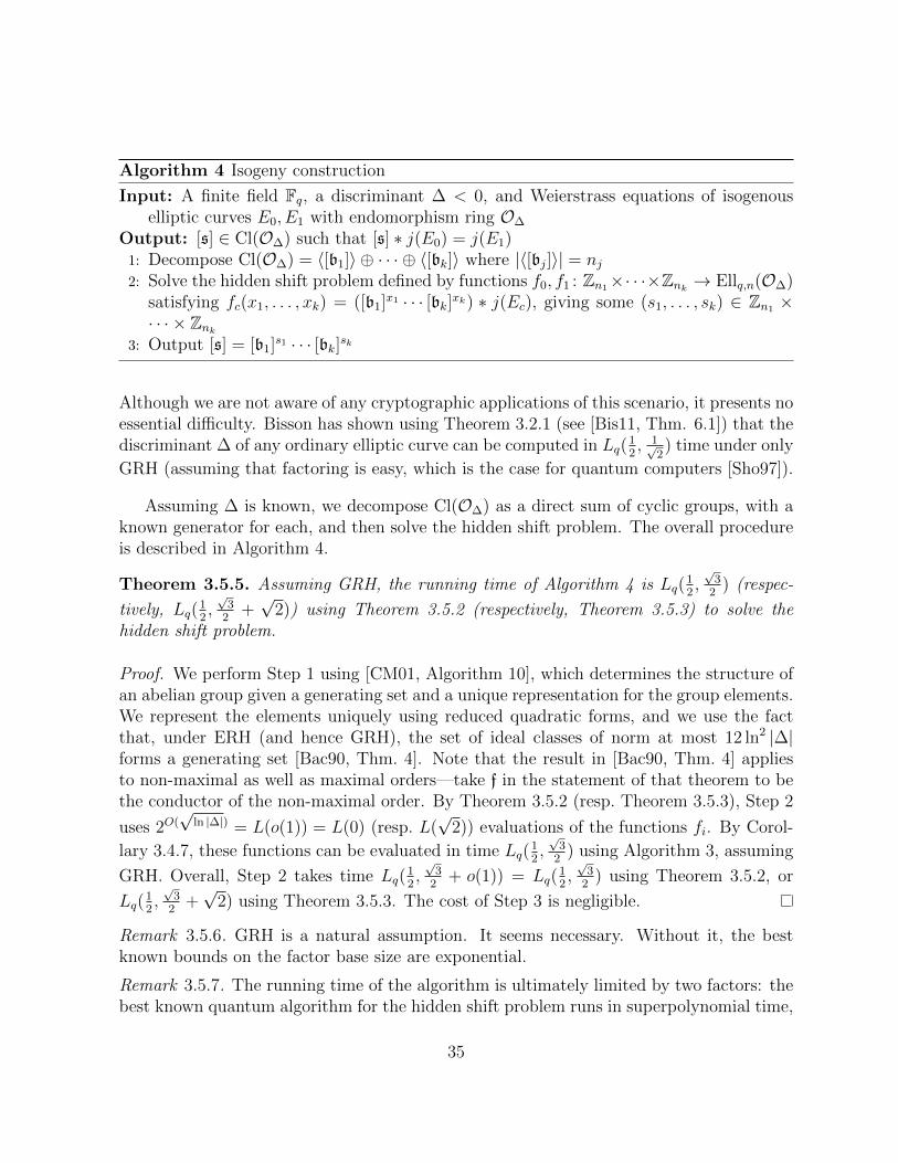
Algorithm 4 Isogeny construction

Input: A finite field Fq, a discriminant ∆ < 0, and Weierstrass equations of isogenouselliptic curves E0, E1 with endomorphism ring O∆

Output: [s] ∈ Cl(O∆) such that [s] ∗ j(E0) = j(E1)1: Decompose Cl(O∆) = 〈[b1]〉 ⊕ · · · ⊕ 〈[bk]〉 where |〈[bj]〉| = nj2: Solve the hidden shift problem defined by functions f0, f1 : Zn1×· · ·×Znk → Ellq,n(O∆)

satisfying fc(x1, . . . , xk) = ([b1]x1 · · · [bk]xk) ∗ j(Ec), giving some (s1, . . . , sk) ∈ Zn1 ×· · · × Znk

3: Output [s] = [b1]s1 · · · [bk]sk

Although we are not aware of any cryptographic applications of this scenario, it presents noessential difficulty. Bisson has shown using Theorem 3.2.1 (see [Bis11, Thm. 6.1]) that thediscriminant ∆ of any ordinary elliptic curve can be computed in Lq(

12, 1√

2) time under only

GRH (assuming that factoring is easy, which is the case for quantum computers [Sho97]).

Assuming ∆ is known, we decompose Cl(O∆) as a direct sum of cyclic groups, with aknown generator for each, and then solve the hidden shift problem. The overall procedureis described in Algorithm 4.

Theorem 3.5.5. Assuming GRH, the running time of Algorithm 4 is Lq(12,√

32

) (respec-

tively, Lq(12,√

32

+√

2)) using Theorem 3.5.2 (respectively, Theorem 3.5.3) to solve thehidden shift problem.

Proof. We perform Step 1 using [CM01, Algorithm 10], which determines the structure ofan abelian group given a generating set and a unique representation for the group elements.We represent the elements uniquely using reduced quadratic forms, and we use the factthat, under ERH (and hence GRH), the set of ideal classes of norm at most 12 ln2 |∆|forms a generating set [Bac90, Thm. 4]. Note that the result in [Bac90, Thm. 4] appliesto non-maximal as well as maximal orders—take f in the statement of that theorem to bethe conductor of the non-maximal order. By Theorem 3.5.2 (resp. Theorem 3.5.3), Step 2

uses 2O(√

ln |∆|) = L(o(1)) = L(0) (resp. L(√

2)) evaluations of the functions fi. By Corol-

lary 3.4.7, these functions can be evaluated in time Lq(12,√

32

) using Algorithm 3, assuming

GRH. Overall, Step 2 takes time Lq(12,√

32

+ o(1)) = Lq(12,√

32

) using Theorem 3.5.2, or

Lq(12,√

32

+√

2) using Theorem 3.5.3. The cost of Step 3 is negligible.

Remark 3.5.6. GRH is a natural assumption. It seems necessary. Without it, the bestknown bounds on the factor base size are exponential.

Remark 3.5.7. The running time of the algorithm is ultimately limited by two factors: thebest known quantum algorithm for the hidden shift problem runs in superpolynomial time,

35

and the same holds for the best known (classical or quantum) algorithm for computing thecomplex multiplication operator. Improving only one of these results to take polynomialtime would still result in a superpolynomial-time algorithm.

36

Chapter 4

Isogeny-Based Quantum-ResistantKey Exchange and Encryption

4.1 Introduction

As part of the background material necessary in order to explain our contributions fromChapters 5 and 6 of this thesis, we describe in this chapter the isogeny-based cryptosystemsof De Feo and Jao [JDF11] and De Feo et al. [DFJP14]. Portions of these publicationswere used in this chapter with permission.

The Diffie-Hellman scheme is a fundamental protocol for public-key exchange betweentwo parties. Its original definition over finite fields is based on the hardness of computingthe map g, ga, gb 7→ gab for g ∈ F∗p. As already discussed in previous chapters, Stol-bunov [Sto10] proposed a Diffie-Hellman type system based on the difficulty of computingisogenies between ordinary elliptic curves, with the stated aim of obtaining quantum-resistant cryptographic protocols. The fastest known (classical) probabilistic algorithm forsolving this problem is the algorithm of Galbraith and Stolbunov [GS11], based on thealgorithm of Galbraith, Hess, and Smart [GHS02]. This algorithm is exponential, with aworst-case running time of O( 4

√q). However, as we have shown in previous chapter (and

our paper [CJS14]), the private keys in Stolbunov’s system can be recovered in subexpo-nential time. Moreover, even if we only use classical attacks in assessing security levels,Stolbunov’s scheme requires 229 seconds (even with precomputation) to perform one keyexchange operation at the 128-bit security level on a desktop PC [Sto10, Table 1].

In this chapter, we will look at isogeny-based key-exchange, encryption, and identifi-cation schemes proposed by De Feo and Jao in [JDF11]. Their primitive achieves perfor-mance on the order of 60 milliseconds at the 128-bit security level (as measured againstthe fastest known quantum attacks) using desktop PCs, making the schemes far faster

37

than Stolbunov’s. In terms of security, their schemes are not vulnerable to our algorithmpresented in Chapter 3, nor to any algorithm of this type, since they are not based on agroup action. The fastest known attacks against those schemes, even on quantum comput-ers, require fully exponential time. The schemes involve new computational assumptionsupon which their quantum resistance is based, and like all new computational assumptions,further study and the passage of time is needed for validation. Nevertheless, we believethe proposal represents a promising candidate for quantum-resistant isogeny-based public-key cryptography. We also use those computational assumptions for developing furtherschemes.

The scheme, presented in Section 4.2, uses isogenies between supersingular ellipticcurves rather than ordinary elliptic curves. The main technical difficulty is that, in thesupersingular case, the endomorphism ring is noncommutative, whereas Diffie-Hellmantype protocols require commutativity. In Sections 4.3 and 4.4 we will see formal statementsof the hardness assumptions and security reductions for the system.

4.1.1 Ramanujan Graphs

Let G = (V , E) be a finite graph on h vertices V with undirected edges E . Suppose G isa regular graph of degree k, i.e., exactly k edges meet at each vertex. Given a labeling ofthe vertices V = {v1, . . . , vh}, the adjacency matrix of G is the symmetric h× h matrix Awhose ij-th entry Ai,j = 1 if an edge exists between vi and vj and 0 otherwise.

It is convenient to identify functions on V with vectors in Rh via this labeling, andtherefore also think of A as a self-adjoint operator on L2(V). All of the eigenvalues of Asatisfy the bound |λ| ≤ k. Constant vectors are eigenfunctions of A with eigenvalue k,which for obvious reasons is called the trivial eigenvalue λtriv. A family of such graphs Gwith h → ∞ is said to be a sequence of expander graphs if all other eigenvalues of theiradjacency matrices are bounded away from λtriv = k by a fixed amount.1 In particular, noother eigenvalue is equal to k; this implies the graph is connected. A Ramanujan graph isa special type of expander which has |λ| ≤ 2

√k − 1 for any nontrivial eigenvalue which is

not equal to −k (this last possibility happens if and only if the graph is bipartite). TheRamanujan property was first defined in [LPS88]. It characterizes the optimal separa-tion between the two largest eigenvalues of the graph adjacency matrix, and implies theexpansion property.

A fundamental use of expanders is to prove the rapid mixing of the random walk on Valong the edges E . The following rapid mixing result is standard but we present it belowfor completeness. For the proof, see [JMV09] or [DSV03, Lub94, Sar90].

1Expansion is usually phrased in terms of the number of neighbors of subsets of G, but the spectralcondition here is equivalent for k-regular graphs and also more useful for our purposes.

38

Proposition 4.1.1. Let G be a regular graph of degree k on h vertices. Suppose that theeigenvalue λ of any nonconstant eigenvector satisfies the bound |λ| ≤ c for some c < k.Let S be any subset of the vertices of G, and x be any vertex in G. Then a random walk of

length at least log 2h/|S|1/2log k/c

starting from x will land in S with probability at least |S|2h

= |S|2|G| .

4.1.2 Isogeny Graphs

An isogeny graph is a graph whose nodes consist of all elliptic curves in Fq belonging to afixed isogeny class, up to Fq-isomorphism (so that two elliptic curves which are isomorphicover Fq represent the same node in the graph). In practice, the nodes are representedusing j-invariants, which are invariant up to isomorphism. Isogeny graphs for supersingularelliptic curves were first considered by Mestre [Mes86], and were shown by Pizer [Piz90,Piz98] to have the Ramanujan property.

Every supersingular elliptic curve in characteristic p is defined over either Fp or Fp2

[Sil92], so it suffices to fix Fq = Fp2 as the field of definition for this discussion. Thus, incontrast to ordinary curves, there are a finite number of isomorphism classes of supersin-gular curves in any given isogeny class; this number is in fact g + 1, where g is the genusof the modular curve X0(p), which is roughly p/12. It turns out that all supersingularcurves defined over Fp belong to the same isogeny class [Mes86]. For a fixed prime valueof ` 6= p, we define the vertices of the supersingular isogeny graph G to consist of theseg + 1 isomorphism classes of curves, with edges given by isomorphism classes of degree-`isogenies, defined as follows: two isogenies φ1, φ2 : Ei → Ej are isomorphic if there existsan automorphism α ∈ Aut(Ej) (i.e., an invertible endomorphism) such that φ2 = αφ1.Pizer [Piz90, Piz98] has shown that G is a connected k = ` + 1-regular multigraph satis-fying the Ramanujan bound of |λ| ≤ 2

√` = 2

√k − 1 for the nontrivial eigenvalues of its

adjacency matrix.

4.2 Public-Key Cryptosystems Based On Supersingu-

lar Curves

In this section we present a key-exchange protocol and a public-key cryptosystem anal-ogous to those of [RS06, Sto10], and a zero-knowledge identification scheme, all usingsupersingular elliptic curves.

The protocols require supersingular curves of smooth order. Such curves are normallyunsuitable for cryptography since discrete logarithms on them are easy. However, since thediscrete logarithm problem is unimportant in our setting, this issue does not affect us. Inthe supersingular setting, it is easy to construct curves of smooth order, and using a smooth

39

order curve will give a large number of isogenies that are fast to compute. Specifically, wefix Fq = Fp2 as the field of definition, where p is a prime of the form `eAA `

eBB · f ± 1. Here

`A and `B are small primes, and f is a cofactor such that p is prime. Then we constructa supersingular curve E defined over Fq of cardinality (`eAA `

eBB f)2. By construction, E[`eAA ]

is Fq-rational and contains `eA−1A (`A + 1) cyclic subgroups of order `eAA , each defining a

different isogeny; the analogous statement holds for E[`eBB ].

The protocols revolve around the following commutative diagram

E E/〈P 〉

E/〈Q〉 E/〈P,Q〉

φ

ψ(4.1)

where φ and ψ are random walks in the graphs of isogenies of degrees `A and `B respectively.Their security is based on the difficulty of finding a path connecting two given vertices ina graph of supersingular isogenies.

4.2.1 Zero-Knowledge Proof of Identity

We begin with the protocol which is easiest to understand. Peggy knows a cyclic degree`eAA isogeny φ : E → E/〈S〉, with the curves E and E/〈S〉 publicly known, and wants toprove to Vic that she knows a generator for 〈S〉, without revealing it.

The protocol is loosely inspired by the zero-knowledge proof of membership for GraphIsomorphism [GMW91]. In that protocol, Peggy shows that she knows a graph isomor-phism G ' G′ by first publishing a random H such that the following diagram commutes

G G′

Hφ ψ

(4.2)

and then revealing only one among φ and ψ. Intuitively, this protocol is perfectly zero-knowledge because the information that Peggy reveals (i.e., a random permutation of Gor G′) could be easily computed by anyone without her help.

In an analogous way, the protocol consists in publishing the vertices of diagram (4.1),and then revealing some, but not all, of its arrows. Unlike the case of Graph Isomorphism,in the protocol Peggy needs to use her secret knowledge to create the diagram, thus wecannot achieve a perfect zero-knowledge. Nevertheless, we will show in Section 4.4 that,under suitable assumptions, the protocol is computationally zero-knowledge.

40

We show below the diagram used in the protocol. 〈S〉 is the kernel of the secret isogenyφ of degree `eAA , while 〈R〉 is a cyclic group of order `eBB .

E E/〈S〉

E/〈R〉 E/〈S,R〉

φ

ψ ψ′

φ′(4.3)

Peggy can compute the diagram as follows:

• She uses Velu’s formulas to compute the isogeny ψ : E → E/〈R〉;

• She computes R′ = φ(R) and the isogeny ψ′ : E/〈S〉 → E/〈S,R〉;

• She computes S ′ = ψ(S) and the isogeny φ′ : E/〈R〉 → E/〈S,R〉.

Now, the natural question is: which arrows of the diagram can Peggy reveal withoutcompromising her secret φ? It is not hard to see, and we will show it in Theorem 4.4.3,that the knowledge of (ψ, φ′) or (ψ′, φ′) allows anyone to compute the kernel of φ. However,we will argue that there is no obvious way to compute φ from the sole knowledge of φ′.Revealing one of ψ or ψ′ is no problem either, however revealing (ψ, ψ′) altogether is moresubtle. Indeed, revealing the points R and φ(R) uncovers some information on the actionof φ on E[`eBB ]: it is to be expected that after a few iterations Peggy will reveal a basis(P,Q) of E[`eBB ] and the respective images φ(P ), φ(Q), thus allowing anyone to evaluateφ on the whole E[`eBB ]. Nevertheless, we conjecture that this leakage does not compromisePeggy’s secret either, and we make these data part of the public parameters.2

Finally, we present the protocol.

Secret parameters A supersingular curve E defined over Fq and a primitive `eAA -torsionpoint S defining an isogeny φ : E → E/〈S〉.

Public parameters The curves E and E/〈S〉. Generators P,Q of E[`eBB ] and their imagesφ(P ), φ(Q).

Identification Repeat m times:

1. Peggy chooses a random point R of order `eBB and computes diagram (4.3).

2An alternative solution, that intuitively leaks less information on φ, would be to publish randomgenerators of 〈R〉 and 〈φ(R)〉. However, it is not clear that this idea would considerably improve thesecurity of the protocol, and we will not pursue it further for coherence with the protocols that will follow.

41

2. Peggy sends the curves E1 = E/〈R〉 and E2 = E/〈S,R〉 to Vic.

3. Vic selects a random bit b and sends it to Peggy.

4. If b = 0, Peggy reveals the points R and R′ = φ(R). Vic accepts if they haveorder `eBB and generate the kernels of isogenies E → E1 and E/〈S〉 → E2,respectively.

5. If b = 1, Peggy reveals the point ψ(S). Vic accepts if it has order `eAA andgenerates the kernel of an isogeny E1 → E2.

4.2.2 Key Exchange

The key exchange protocol is a variation a la Diffie-Hellman over diagram (4.1). The idea isto let Alice choose φ, while Bob chooses ψ. Although similar in spirit to the protocol basedon the action of the class group on ordinary elliptic curves of [Sto10], a main technicaldifference is that, since ideal classes no longer commute (or indeed even multiply together)in the supersingular case, extra information must be communicated as part of the protocolin order to ensure that both parties arrive at the same common value.

We fix as public parameters a supersingular curve E0 defined over Fp2 , and bases{PA, QA} and {PB, QB} which generate E0[`eAA ] and E0[`eBB ] respectively, so that 〈PA, QA〉 =E0[`eAA ] and 〈PB, QB〉 = E0[`eBB ]. Note that all torsion groups are always defined overFp2 , hence this requires picking a curve having the correct order over Fp2 . Alice choosestwo random elements mA, nA ∈R Z/`eAA Z, not both divisible by `A, and computes anisogeny φA : E0 → EA with kernel KA := 〈[mA]PA + [nA]QA〉. Alice also computesthe image {φA(PB), φA(QB)} ⊂ EA of the basis {PB, QB} for E0[`eBB ] under her secretisogeny φA, and sends these points to Bob together with EA. Similarly, Bob selects ran-dom elements mB, nB ∈R Z/`eBB Z and computes an isogeny φB : E0 → EB having kernelKB := 〈[mB]PB + [nB]QB〉, along with the points {φB(PA), φB(QA)}. Upon receipt of EBand φB(PA), φB(QA) ∈ EB from Bob, Alice computes an isogeny φ′A : EB → EAB havingkernel equal to 〈[mA]φB(PA) + [nA]φB(QA)〉; Bob proceeds mutatis mutandis. Alice andBob can then use the common j-invariant of

EAB = φ′B(φA(E0)) = φ′A(φB(E0)) = E0/〈[mA]PA+[nA]QA,[mB ]PB+[nB ]QB〉

to form a secret shared key.

The full protocol is given in Figure 4.1. We denote by A and B the identifiers of Aliceand Bob, and use sID to denote the unique session identifier.

42

A BInput: A,B, sID Input: BmA, nA ∈R Z/`eAA Z mB, nB ∈R Z/`eBB ZφA := E0/〈[mA]PA+[nA]QA〉 φB := E0/〈[mB ]PB+[nB ]QB〉

A,sIDφA(PB),φA(QB),EA−−−−−→B,sIDφB(PA),φB(QA),EB←−−−−−

EAB := EBA :=EB/〈[mA]φB(PA)+[nA]φB(QA)〉 EA/〈[mB ]φA(PB)+[nB ]φA(QB)〉

Output: j(EAB), sID Output: j(EBA), sID

E0

EA

ker(φA

)=〈[mA

]PA+[nA

]QA〉

φA(PB

),φA(QB

)

EB

ker(φB )=〈[m

B ]PB+[n

B ]QB 〉

φB (P

A ),φB (Q

A )

EAB

ker(φ′A

)=〈[mA

]φB(PA

)+[nA]φB

(QA)〉

EBA

ker(φ ′B )=〈[m

B ]φA (P

B )+[nB ]φ

A (QB )〉

‖

Figure 4.1: Key-exchange protocol using isogenies on supersingular curves.

4.2.3 Public-Key Encryption

The key-exchange protocol of Section 4.2.2 can easily be adapted to yield a public-keycryptosystem, in much the same way that Elgamal encryption follows from Diffie-Hellman.We briefly give the details here. All notation is the same as above. Stolbunov [Sto10] usesa similar construction, upon which this one is based.

Setup Choose p = `eAA `eBB ·f±1, E0, {PA, QA}, {PB, QB} as above. Let H = {Hk : k ∈ K}

be a hash function family indexed by a finite set K, where each Hk is a function fromFp2 to the message space {0, 1}w.

Key generation Choose two random elements mA, nA ∈R Z/`eAA Z, not both divisible by`A. Compute EA, φA(PB), φA(QB) as above, and choose a random element k ∈R

43

K. The public key is the tuple (EA, φA(PB), φA(QB), k) and the private key is(mA, nA, k).

Encryption Given a public key (EA, φA(PB), φA(QB), k) and a message m ∈ {0, 1}w,choose two random elements mB, nB ∈R Z/`eBB Z, not both divisible by `B, and com-pute

h = Hk(j(EAB)),

c = h⊕m.

The ciphertext is (EB, φB(PA), φB(QA), c).

Decryption Given a ciphertext (EB, φB(PA), φB(QA), c) and a private key (mA, nA, k),compute the j-invariant j(EAB) and set

h = Hk(j(EAB)),

m = h⊕ c.

The plaintext is m.

For detail on the algorithmic aspects of the schemes, please refer to the original paper.

4.3 Complexity Assumptions

As before, let p be a prime of the form `eAA `eBB · f ± 1, and fix a supersingular curve E0

over Fp2 together with bases {PA, QA} and {PB, QB} of E0[`eAA ] and E0[`eBB ] respectively.In analogy with the case of isogenies over ordinary elliptic curves, we define the followingcomputational problems, adapted for the supersingular case:

Problem 4.3.1 (Decisional Supersingular Isogeny (DSSI) problem). Let EA be another su-persingular curve defined over Fp2 . Decide whether EA is `eAA -isogenous to E0.

Problem 4.3.2 (Computational Supersingular Isogeny (CSSI) problem). Fix an isogenyφA : E0 → EA whose kernel is 〈[mA]PA + [nA]QA〉, where mA and nA are chosen at randomfrom Z/`eAA Z and not both divisible by `A. Given EA and the values φA(PB), φA(QB), finda generator RA of 〈[mA]PA + [nA]QA〉.

We remark that given a generator RA = [mA]PA + [nA]QA, it is easy to solve for(mA, nA), since E0 has smooth order and thus extended discrete logarithms are easy inE0 [Tes99].

44

Problem 4.3.3 (Supersingular Computational Diffie-Hellman (SSCDH) problem). Fix anisogeny φA : E0 → EA whose kernel is equal to 〈[mA]PA + [nA]QA〉, and let φB : E0 → EBbe an isogeny whose kernel is 〈[mB]PB + [nB]QB〉, where mA, nA (respectively mB, nB)are chosen at random from Z/`eAA Z (respectively Z/`eBB Z) and not both divisible by `A(respectively `B). Given the curves EA, EB and the points φA(PB), φA(QB), φB(PA),φB(QA), find the j-invariant of E0/〈[mA]PA + [nA]QA, [mB]PB + [nB]QB〉.Problem 4.3.4 (Supersingular Decisional Diffie-Hellman (SSDDH) problem). Given a tuplesampled with probability 1/2 from one of the following two distributions:

• (EA, φA(PB), φA(QB), EB, φB(PA), φB(QA), EAB), where the quantities EA, φA(PB),φA(QB), EB, φB(PA), and φB(QA) are as in the SSCDH problem and

EAB ∼= E0/〈[mA]PA + [nA]QA, [mB]PB + [nB]QB〉,

• (EA, φA(PB), φA(QB), EB, φB(PA), φB(QA), EC), wherein the quantities EA, φA(PB),φA(QB), EB, φB(PA), and φB(QA) are as in the SSCDH problem and

EC ∼= E0/〈[m′A]PA + [n′A]QA, [m′B]PB + [n′B]QB〉,

where m′A, n′A (respectively m′B, n

′B) are chosen at random from Z/`eAA Z (respectively

Z/`eBB Z) and not both divisible by `A (respectively `B),

determine from which distribution the tuple is sampled.

The ordinary case analogue of the following problem is trivially solvable in polynomialtime. Its supposed difficulty in the supersingular case is at the heart of the security of thisidentification scheme.

Problem 4.3.5 (Decisional Supersingular Product (DSSP) problem). Given a degree `eAAisogeny φ : E0 → E3 and a tuple sampled with probability 1/2 from one of the followingtwo distributions:

• (E1, E2, φ′), where the productE1×E2 is chosen at random among those `eBB -isogenous

to E0 × E3, and where φ′ : E1 → E2 is an isogeny of degree `eAA , and

• (E1, E2, φ′), where E1 is chosen at random among the curves having the same cardi-

nality as E0, and φ′ : E1 → E2 is a random isogeny of degree `eAA ,

determine from which distribution the tuple is sampled.

We conjecture that these problems are computationally infeasible, in the sense thatfor any polynomial-time solver algorithm, the advantage of the algorithm is a negligiblefunction of the security parameter log p. The resulting security assumptions are referredto as the DSSI assumption, CSSI assumption, etc.

45

4.3.1 Hardness Of The Underlying Assumptions

In this section we discuss the feasibality of solving isogeny-based computational problemson a quantum computer. At a high level, the fastest known attacks against CSSI, DSSPinvolve claw-finding in the isogeny graph. Known existing lower bounds for quantum claw-finding provide some assurance that a faster attack will never be found since such anattack would require a non-generic solutions to the claw-finding problem. The lack of anyrelated commutative group structure or periodic function in the isogeny graph indicatesthat analogues to Shor’s algorithm are unlikely to apply to isogeny computation.

Given a CSSI (respectively, SSCDH) solver, it is trivial to solve SSCDH (respectively,SSDDH). It is also trivial to solve SSDDH given a DSSI solver. There are no knownreductions in the other direction, and given that the corresponding question of equivalencefor discrete logarithms and Diffie-Hellman has not yet been completely resolved in all cases,it is reasonable to assume that the question of equivalence of CSSI, SSCDH, and SSDDHis at least hard to resolve. For the purposes of this discussion, we will presume that DSSIand CSSI are equivalent to SSDDH. Concerning DSSP, there is an evident reduction toDSSI. However, it seems reasonable to assume that DSSP is easier than the latter.

In the context of cryptography, the problem of computing an isogeny between isoge-nous supersingular curves was first considered by Galbraith [Gal99] in 1999. The firstpublished cryptographic primitive based on supersingular isogeny graphs is the hash func-tion proposal of Charles et al. [CLG09], which remains unbroken to date (the cryptanalysisof [PLQ08] applies only to the LPS graph-based hash function from [CLG09], and not tothe supersingular isogeny graph-based hash functions). The fastest known algorithm forfinding isogenies between supersingular curves in general takes O(

√p log2 p) time [CLG09,

§5.3.1]; however the presented problem is less general because the degree of the isogenyis known in advance and is smooth. In addition, the distribution of isogenous curves ob-tained from taking kernels of the form 〈[mA]PA + [nA]QA〉 is not quite uniform: a simplecalculation against Proposition 4.1.1 indicates that a sequence of eA isogenies of degree`A falls short of the length needed to ensure uniform mixing, regardless of the value of p.Since our research group is the first to propose using isogenies of this type, there is noexisting literature addressing the security of the isogenies of the special form proposed.

There are easy exponential attacks against DSSI and CSSI that improve upon exhaus-tive search. To find an isogeny of degree `eAA between E and EA, an attacker builds two

trees of all curves isogenous to E (respectively, EA) via isogenies of degree `eA/2A . Once the

trees are built, the attacker tries to find a curve lying in both trees. Since the degree ofthe isogeny φA is ∼ √p (much shorter than the size of the isogeny graph), it is unlikelythat there will be more than one isogeny path—and thus more than one match—fromE to EA. Given two functions f : A → C and g : B → C with domain of equal size,finding a pair (a, b) such that f(a) = g(b) is known as the claw problem in complexity

46

theory. The claw problem can obviously be solved in O(|A| + |B|) time and O(|A|) spaceon a classical computer by building a hash table holding f(a) for any a ∈ A and looking

for hits for g(b) where b ∈ B. This gives a O(`eA/2A ) = O( 4

√p) classical attack against

those cryptosystems. With a quantum computer, one can do better using the algorithmin [Tan08], which has complexity O( 3

√|A||B|), thus giving an O(`

eA/3A ) = O( 6

√p) quantum

attack against the presented cryptosystems. These complexities are optimal for a black-boxclaw attack [Zha05].

We consider the question of whether the auxiliary data points φA(PB) and φA(QB)might assist an adversary in determining φA. Since (PB, QB) forms a basis for E0[`eBB ], thevalues φA(PB) and φA(QB) allow the adversary to compute φA on all of E0[`eBB ]. This isbecause any element of E0[`eBB ] is a (known) linear combination of PB and QB (known sinceextended discrete logarithms are easy [Tes99]). However, there does not appear to be anyway to use this capability to determine φA. Even on a quantum computer, where findingabelian hidden subgroups is easy, there is no hidden subgroup to find, since φA has degree`eAA , and thus does not annihilate any point in E0[`eBB ] other than the identity. Of course,if one could evaluate φA on arbitrary points of E0[`eAA ], then a quantum computer couldeasily break the scheme, and indeed in this case the scheme is also easily broken classicallyby using a few calls to the oracle to compute a generator of the kernel of the dual isogenyφA. However, it does not seem possible to translate the values of φA on E0[`eBB ] into valueson E0[`eAA ].

Recall that, for both ordinary and supersingular curves, there is a natural bijectionbetween isogenies (up to isomorphism) and (left) ideals in the endomorphism ring. In theordinary case the endomorphism ring is commutative, and ideal classes form a finite abeliangroup. This property has been used by Childs et al. [CJS14] to solve the ordinary analogueof CSSI in quantum subexponential time. It is natural to ask whether their algorithm canbe adapted to the supersingular setting. Here the endomorphism ring is a maximal orderin a noncommutative quaternion algebra, and the left ideal classes do not form a group atall (though they do form a groupoid). Since the algorithm of Childs et al. depends cruciallyon the properties of abelian groups, we believe that no reasonable variant of this strategywould apply.

The same correspondence between isogenies and ideals can be applied to DSSP. Indeed,deciding DSSP amounts to deciding whether the ideals S, S ′ associated to φ, φ′ are conju-gated, i.e., whether there exists a left ideal R ∈ End(E0) such that S = RS ′R−1. Althoughit can be hoped that deciding conjugacy of ideal classes in the quaternion algebra Qp,∞ isfeasible, we are still faced with the problem that the best known algorithms to compute theendomorphism rings of supersingular curves are exponential in log p [Koh96, Cn04, Bel08].Hence, we deem DSSP secure given the current knowledge.

The fact that it is possible to obtain a zero-knowledge identification scheme from CSSIcomes as no surprise, since it is well known that a zero-knowledge protocol can be ob-

47

tained from any problem in NP [GMW91]. Nevertheless, the generic construction is notvery efficient, and many efforts have been made to obtain efficient ad-hoc schemes fromNP-complete problems [Sha89, Ste94a, Ste94b, Poi95]. While the security of most of theseschemes is based on two solid assumptions, namely that P 6= NP and that secure commit-ment schemes exist, the presented identification scheme stands on a much weaker ground:the CSSI and DSSP problems. As performances go, it is reasonable to assume that thepresented scheme will be some orders of magnitude slower than the best zero-knowledgeprotocols. We can thus conclude that presented scheme is of a purely theoretical andpedagogical interest. Yet it is remarkable that an efficient identification scheme based ongraphs of supersingular isogenies simply exists, while the analogous construction for ordi-nary curves is trivially broken and no other identification scheme is currently known towork in that case [Sto10].

4.4 Security Results

In this section we state the security results for the schemes presented in this chapter. Thestatements of the theorems are as follows:

Theorem 4.4.1. If the SSDDH assumption holds, then the key-agreement protocol of Sec-tion 4.2.2 is session-key secure in the authenticated-links adversarial model of Canetti andKrawczyk [CK01].

Theorem 4.4.2. If the SSDDH assumption holds, and the hash function family H isentropy-smoothing, then the public-key cryptosystem of Section 4.2.3 is IND-CPA.

Theorem 4.4.3. Under the CSSI and DSSP assumptions, the identification scheme ofSection 4.2.1 is zero-knowledge.

For proofs of the theorems, we refer to the original paper [JDF11].

48

Chapter 5

Isogeny-Based Quantum-ResistantUndeniable Signatures

5.1 Introduction

This chapter is based on [JS14], authored jointly with my supervisor David Jao.

Many current cryptographic schemes are based on mathematical problems that areconsidered difficult with classical computers, but can easily be solved using quantum al-gorithms. To prepare for the emergence of quantum computers, we aim to design cryp-tographic primitives for common operations such as encryption and authentication whichresist quantum attacks. One family of such primitives, proposed by De Feo, Jao, andPlut [DFJP14, JDF11], which we described in the previous chapter, uses isogenies betweensupersingular elliptic curves to construct cryptographic protocols for public-key encryp-tion, key exchange, and entity authentication which are believed to be quantum-resistant.To date, however, this protocol family lacks comprehensive techniques for achieving dataauthentication.

In this chapter, we present a new construction of quantum-resistant undeniable signa-tures based on the difficulty of computing isogenies between supersingular elliptic curves.Few such constructions are known, and indeed the only other proposed quantum-resistantundeniable signature scheme in the literature is the code-based scheme of Aguilar-Melchoret al. [AMBGS13]. Our scheme uses a completely different approach and is based oncompletely different assumptions, making it a useful alternative in the event that somebreakthrough arises in the cryptanalysis of code-based systems.

Undeniable signatures provide tools for signer to prove that the signature is valid fora given message, if it was truly signed by him. If the signature is fake, the signer has thetools to prove that it is fake.

49

5.2 Quantum-Resistant Undeniable Signatures From

Isogenies

In this section, we present a new construction of an undeniable signature scheme fromisogenies. An undeniable signature can be verified by any party, but verification requiresinteraction with the signer. To distinguish between invalid (forged) signatures and validsignatures that the verifier refuses to verify, an undeniable signature scheme also includesa mechanism for the signer to prove (interactively) that an invalid signature is forged.Our construction uses a three-prime variant of the original two-prime protocol given inSection 4.2.2. As a consequence, the resulting commutative diagrams for zero-knowledgeproofs become 3-dimensional rather than 2-dimensional.

5.2.1 Definition

An undeniable signature scheme [KF08] consists of a key generation algorithm, a signingalgorithm, a validity check, a signature simulator, a confirmation protocol πcon and adisavowal protocol πdis. The role of the confirmation protocol πcon is for the signer to proveto the verifier that the signature is valid. The role of the disavowal protocol πdis is fora valid signer to be able to prove to the verifier that the signature that the verifier hasreceived is not valid.

Unforgeability is defined using the following game between a challenger and an adversaryA.

1. The challenger generates a key pair (vk, sk) randomly, and gives the verification keyvk to A.

2. For i = 1, 2, . . . , qs for some qs, A queries the signing oracle adaptively with a messagemi and receives a signature σi.

3. Eventually, A outputs a forgery (m∗, σ∗).

We also allow the adversary A to submit pairs (mj, σj) to the confirmation/disavowal oracleadaptively in step 2, where the confirmation/disavowal oracle responds as follows:

• If (mj, σj) is a valid pair, then the oracle returns a bit µ = 1 and proceeds with theexecution of the confirmation protocol πcon with A.

• Otherwise, the oracle returns a bit µ = 0 and proceeds with the execution of thedisavowal protocol πdis with A.

50

We say that A succeeds in producing a strong forgery if (m∗, σ∗) is valid and (m∗, σ∗) isnot among the pairs (mi, σi) generated during the signing queries. The signature schemeis strongly unforgeable if the probability that A succeeds in producing a strong forgery isnegligible for any PPT adversary A in the above game.

Invisibility is defined using the following game between a challenger and an adversaryA.

1. The challenger generates a key pair (vk, sk) randomly, and gives the verification keyvk to A.

2. A is permitted to issue a series of signing queries mi to the signing oracle adaptivelyand receive a signature σi.

3. At some point, A chooses a message m∗ and sends it to the challenger.

4. The challenger chooses a random bit b. If b = 1, then he computes the real signaturefor m∗ using sk and sets it to be σ∗. Otherwise he computes a fake signature m∗

using vk and sets it to be σ∗. He sends σ∗ to A.

5. A performs some signing queries again.

6. At the end of this game, A outputs a guess b′.

We allow the adversary A to submit pairs (mj, σj) to the confirmation/disavowal oracleadaptively in step 2 and in step 5. However, A is not allowed to submit the challenge(m∗, σ∗) to the confirmation/disavowal oracle in step 5. Also, A is not allowed to submitm∗ to the signing oracle. We say that the signature scheme is invisible if no PPT adversaryA has non-negligible advantage in this game.

For an undeniable signature scheme to be secure, it must satisfy unforgeability and in-visibility. In addition, the confirmation πcon and disavowal πdis protocols must be complete,sound, and zero-knowledge.

5.2.2 Protocol

Let p be a prime of the form `eAA `eMM `eCC · f ± 1, and fix a supersingular curve E over

Fp2 together with bases {PA, QA}, {PM , QM} and {PC , QC} of E[`eAA ], E[`eMM ] and E[`eCC ]respectively. The design of the protocol is such that, generally speaking, points in 〈PA, QA〉are used for key material, points in 〈PM , QM〉 are used for message data, and points in〈PC , QC〉 correspond to commitment data.

The signer generates two secret random integers mA, nA ∈ Z/`eAA Z, obtains KA =[mA]PA + [nA]QA and computes EA = E/〈KA〉. Let φA be an isogeny from E to EA.

51

Public parameters: p, E, {PA, QA}, {PM , QM}, {PC , QC}, and a public hash functionH : {0, 1}∗ → Z.

Public key: EA, φA(PC), φA(QC).

Private key: mA, nA.

To sign a message M , we compute the hash h = H(M). Let KM = PM + [h]QM . Thenthe signer computes the isogenies

• φM : E → EM = E/〈KM〉

• φM,AM : EM → EAM = EM/〈φM(KA)〉

• φA,AM : EA → EAM = EA/〈φA(KM)〉

along with the auxiliary points φM,AM(φM(PC)) and φM,AM(φM(QC)). The signer thenpresents these two auxiliary points along with EAM as the signature. (See Figure 5.1.)

The confirmation protocol proceeds as follows. We must confirm EAM without revealingthe isogenies used to produce it. We do so by “blinding” EAM using φC and disclosing theblinded isogenies (see Figure 5.2).

EA

E

EAM

EM

φA,AM

φA

φM

φM,AM

Figure 5.1: Signature generation.

EA EAC

E EC

EAM EAMC

EM EMC

φA,AC

φA,AM

φAC,AMC

φA

φC

φM φAM,AMC

φM,AM

φM,MC

φMC,AMC

φC,MC

φC,AC

Figure 5.2: Confirmation protocol.

1. The signer secretly selects random integers mC , nC ∈ Z/`eCC Z, and computes the pointKC = [mC ]PC + [nC ]QC together with the curves and isogenies in Figure 5.2. HereEC = E/〈KC〉, EMC = EM/〈φM(KC)〉 = EC/〈φC(KM)〉, EAC = EA/〈φA(KC)〉 =EC/〈φC(KA)〉, and EAMC = EMC/〈φC,MC(KA)〉.

2. The signer outputs EC , EAC , EMC , EAMC , and ker(φC,MC) as the commitment.

3. The verifier randomly selects b ∈ {0, 1}.

52

4. If b = 0, the signer outputs ker(φC). Using the signer’s public key, the verifiercomputes ker(φA,AC). Using knowledge of ker(φM), the verifier computes φM,MC .Using the auxiliary points given as part of the signature, the verifier can computeφAM,AMC . The verifier checks that each isogeny maps between the corresponding twocurves specified in the commitment. Using knowledge of ker(φC), the verifier alsoindependently re-computes φC,MC and checks that it matches the commitment.

5. If b = 1, the signer outputs ker(φC,AC). The verifier computes φMC,AMC and φAC,AMC ,and checks that each of φC,AC , φMC,AMC , and φAC,AMC maps between the correspond-ing two curves specified in the commitment.

We now describe the disavowal protocol. Suppose the signer is presented with a falsifiedsignature (EF , FP , FQ) for a message M , where EF is the falsified EAM , and {FP , FQ}are the falsified auxiliary points corresponding to φM,AM(φM(PC)) and φM,AM(φM(QC))respectively. We must disavow EF without disclosing EAM . To do this, we blind EAM asbefore to obtain EAMC , and disclose enough information to allow the verifier to computeEFC and check that EFC 6= EAMC .

1. The signer secretly selects random integers mC , nC ∈ Z/`eCC Z, and computes KC =[mC ]PC + [nC ]QC along with all the curves and isogenies in Figure 5.3.

2. The signer outputs EC , EAC , EMC , EAMC , and ker(φC,MC) as the commitment.

3. The verifier randomly selects b ∈ {0, 1}.

4. If b = 0, the signer outputs ker(φC). The verifier computes φC , φM,MC , φA,AC ,and φF : EF → EFC = EF/〈[mC ]FP + [nC ]FQ〉, and checks that each isogeny mapsbetween the corresponding two curves specified in the commitment. The verifierindependently re-computes φC,MC and checks that it matches the commitment. Theverifier also checks that EFC 6= EAMC .

5. If b = 1, the signer outputs ker(φC,AC). The verifier computes φAC,AMC and φMC,AMC ,and checks that these isogenies map to EAMC .

53

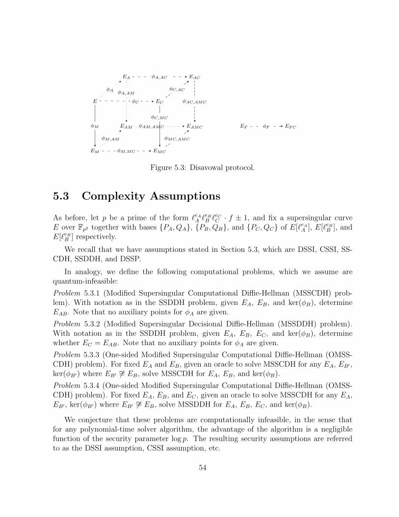
EA EAC

E EC

EAM EAMC EF EFC

EM EMC

φA,AC

φA,AM

φAC,AMC

φA

φC

φM φAM,AMC

φM,AM

φM,MC

φMC,AMC

φC,MC

φC,AC

φF

Figure 5.3: Disavowal protocol.

5.3 Complexity Assumptions

As before, let p be a prime of the form `eAA `eBB `

eCC · f ± 1, and fix a supersingular curve

E over Fp2 together with bases {PA, QA}, {PB, QB}, and {PC , QC} of E[`eAA ], E[`eBB ], andE[`eBB ] respectively.

We recall that we have assumptions stated in Section 5.3, which are DSSI, CSSI, SS-CDH, SSDDH, and DSSP.

In analogy, we define the following computational problems, which we assume arequantum-infeasible:

Problem 5.3.1 (Modified Supersingular Computational Diffie-Hellman (MSSCDH) prob-lem). With notation as in the SSDDH problem, given EA, EB, and ker(φB), determineEAB. Note that no auxiliary points for φA are given.

Problem 5.3.2 (Modified Supersingular Decisional Diffie-Hellman (MSSDDH) problem).With notation as in the SSDDH problem, given EA, EB, EC , and ker(φB), determinewhether EC = EAB. Note that no auxiliary points for φA are given.

Problem 5.3.3 (One-sided Modified Supersingular Computational Diffie-Hellman (OMSS-CDH) problem). For fixed EA and EB, given an oracle to solve MSSCDH for any EA, EB′ ,ker(φB′) where EB′ 6∼= EB, solve MSSCDH for EA, EB, and ker(φB).

Problem 5.3.4 (One-sided Modified Supersingular Computational Diffie-Hellman (OMSS-CDH) problem). For fixed EA, EB, and EC , given an oracle to solve MSSCDH for any EA,EB′ , ker(φB′) where EB′ 6∼= EB, solve MSSDDH for EA, EB, EC , and ker(φB).

We conjecture that these problems are computationally infeasible, in the sense thatfor any polynomial-time solver algorithm, the advantage of the algorithm is a negligiblefunction of the security parameter log p. The resulting security assumptions are referredto as the DSSI assumption, CSSI assumption, etc.

54

We also need a heuristic assumption concerning the distribution of blinded false signa-tures:

Assumption 5.3.5. Fix a supersingular elliptic curve E, an `eAA -isogeny φA, an `eBB -isogenyφB, and a curve EF , not isomorphic to EAB. For any pair of points {P,Q} in EF , only anegligibly small fraction of integer pairs mC , nC satisfyEF/〈mCP + nCQ〉 = EAB/〈φB,AB(φB(mCPC + nCQC))〉.

This assumption is desirable, as in the disavowal protocol, it should be intractable tofind mC , nC such that we obtain a map EF → EABC . This assumption makes sense, as theadversary does not have sufficient information to obtain that map, as the curves EFC andEABC would be independent of each other. This assumption has also been computationallytested.

5.3.1 Hardness Of The Underlying Assumptions

All of our unmodified complexity assumptions (those not containing “Modified” in thename) are identical to the corresponding assumptions from [DFJP14, JDF11], except thatour assumptions are formulated using primes of the form p = `eAA `

eBB `

eCC · f ± 1, rather than

primes of the form p = `eAA `eBB · f ± 1. We have no reason to believe that this alteration

would affect the validity of these assumptions. A close analogy to this situation is thecomparison between three-prime RSA and two-prime RSA, where the use of three-primeRSA incurs some efficiency loss but no known security concerns.

Our modified assumptions are needed in order to prove the security of our undeniablesignature scheme. The MSSCDH and MSSDDH assumptions are complementary to theSSCDH and SSDDH assumptions, with the main difference being that the input consists ofa kernel but not a pair of auxiliary points (rather than the other way around). We believethese assumptions are credible and comparable to SSCDH/SSDDH. The OMSSCDH andOMSSDDH assumptions are somewhat more artificial, and more study will be needed tojustify confidence in them. They arise naturally in the analysis of our undeniable signaturescheme.

Our heuristic assumption (Assumption 5.3.5) seems quite natural, and we have con-ducted numerous empirical experiments confirming it in practice. It would in fact be quitesurprising if the assumption failed to hold. However, we have not yet succeeded in findinga proof of the assumption.

55

5.4 Security Proofs

To prove the security of our scheme, we must show that the confirmation and disavowalprotocols are complete, sound and zero-knowledge, and that the overall scheme satisfiesthe unforgeability and invisibility properties.

The basic principle behind the proofs is that, as was the case in the basic key-exchangeprotocol (Section 4.2.2), knowledge of (the kernels of) any two opposite-side isogenies lyingin a given cube face reveals no information about the other edges in the cube, by the DSSIand DSSP assumptions. On the other hand, knowledge of any two adjacent isogenies ina given commutative square yields full information about all the isogenies in the square.It does not matter which direction the arrows point, since one can reverse the direction ofany arrow using dual isogenies.

Remark 5.4.1. To compute the dual isogeny of an isogeny φ : E → EA = E/〈A〉 whosekernel is generated by a point A, pick any point B ∈ E \ 〈A〉, and compute φ(B). Thenφ(B) generates a kernel subgroup whose corresponding isogeny φ′ : EA → E = EA/〈φ(B)〉is isomorphic to the dual isogeny φ. In general, EA/〈φ(B)〉 is isomorphic but not equal toE, so we also need to compute the appropriate isomorphism, but computing isomorphismsin general is known to be easy [Gal99].

5.4.1 Confirmation Protocol

We need to prove three things: completeness, soundness and zero-knowledge. We applyclassical techniques from [FFS88, GMW91].

Proof of completeness. Completeness for this protocol is obvious. Using the algorithmpresented in Section 5.2.2, the signer can always compute the diagram in Figure 5.2 andmake the verifier accept.

Proof of soundness. Let Charles be a cheating prover that is able to convince the verifierwith non-negligible probability. We also assume that Charles is polynomially bounded.We treat Charles as a black-box that we can control in the sense that we can restart ita polynomial number of times on the same input and each time ask a different set ofquestions. We can then learn with high probability the diagram in Figure 5.4. Knowingthis diagram, we can compute ker(φA), since we know 3 out of 4 edges in the top face. Wethen have full knowledge of φA, and can then trivially solve the MCSSI problem for theleft face.

Proof of zero-knowledge. We show how a cheating verifier (CV) can construct a simulatorS. The simulator S makes uniformly random guesses about what the verifier’s challenge

56

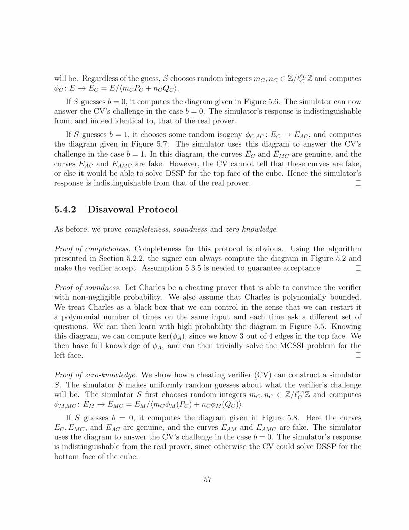
will be. Regardless of the guess, S chooses random integers mC , nC ∈ Z/`eCC Z and computesφC : E → EC = E/〈mCPC + nCQC〉.

If S guesses b = 0, it computes the diagram given in Figure 5.6. The simulator can nowanswer the CV’s challenge in the case b = 0. The simulator’s response is indistinguishablefrom, and indeed identical to, that of the real prover.

If S guesses b = 1, it chooses some random isogeny φC,AC : EC → EAC , and computesthe diagram given in Figure 5.7. The simulator uses this diagram to answer the CV’schallenge in the case b = 1. In this diagram, the curves EC and EMC are genuine, and thecurves EAC and EAMC are fake. However, the CV cannot tell that these curves are fake,or else it would be able to solve DSSP for the top face of the cube. Hence the simulator’sresponse is indistinguishable from that of the real prover.

5.4.2 Disavowal Protocol

As before, we prove completeness, soundness and zero-knowledge.

Proof of completeness. Completeness for this protocol is obvious. Using the algorithmpresented in Section 5.2.2, the signer can always compute the diagram in Figure 5.2 andmake the verifier accept. Assumption 5.3.5 is needed to guarantee acceptance.

Proof of soundness. Let Charles be a cheating prover that is able to convince the verifierwith non-negligible probability. We also assume that Charles is polynomially bounded.We treat Charles as a black-box that we can control in the sense that we can restart ita polynomial number of times on the same input and each time ask a different set ofquestions. We can then learn with high probability the diagram in Figure 5.5. Knowingthis diagram, we can compute ker(φA), since we know 3 out of 4 edges in the top face. Wethen have full knowledge of φA, and can then trivially solve the MCSSI problem for theleft face.

Proof of zero-knowledge. We show how a cheating verifier (CV) can construct a simulatorS. The simulator S makes uniformly random guesses about what the verifier’s challengewill be. The simulator S first chooses random integers mC , nC ∈ Z/`eCC Z and computesφM,MC : EM → EMC = EM/〈mCφM(PC) + nCφM(QC)〉.

If S guesses b = 0, it computes the diagram given in Figure 5.8. Here the curvesEC , EMC , and EAC are genuine, and the curves EAM and EAMC are fake. The simulatoruses the diagram to answer the CV’s challenge in the case b = 0. The simulator’s responseis indistinguishable from the real prover, since otherwise the CV could solve DSSP for thebottom face of the cube.

57

If S guesses b = 1, it chooses some random isogeny φC,AC : EC → EAC , and computesthe diagram given in Figure 5.9. The simulator uses this diagram to answer the CV’schallenge in the case b = 1. In this diagram, the curves EC and EMC are genuine, and thecurves EAC and EAMC are fake. However, the CV cannot tell that these curves are fake,or else it would be able to solve DSSP for the top face of the cube. Hence the simulator’sresponse is indistinguishable from that of the real prover.

EA EAC

E EC

EAM EAMC

EM EMC

φA,AC

φAC,AMCφC

φM φAM,AMC

φM,MC

φMC,AMC

φC,MC

φC,AC

Figure 5.4: Proof of soundness (confirma-tion)

EA EAC

E EC

EAM EAMC

EM EMC

φA,AC

φAC,AMCφC

φM

φM,MC

φMC,AMC

φC,MC

φC,AC

Figure 5.5: Proof of soundness (disavowal)

EA EAC

E EC

EAM EAMC

EM EMC

φA,AC

φC

φM φAM,AMC

φM,MC

φC,MC

Figure 5.6: Confirmation (b = 0 case)

EA EAC

E EC

EAM EAMC

EM EMC

φAC,AMC

φM

φMC,AMC

φC,MC

φC,AC

Figure 5.7: Confirmation (b = 1 case)

EA EAC

E EC

EAM EAMC

EM EMC

φA,AC

φC

φM φAM,AMC

φM,MC

φC,MC

Figure 5.8: Disavowal (b = 0 case)

EA EAC

E EC

EAMC

EM EMC

φAC,AMC

φM

φMC,AMC

φC,MC

φC,AC

Figure 5.9: Disavowal (b = 1 case)58

5.4.3 Unforgeability and Invisibility

Finally, we prove that the protocol satisfies the unforgeability and invisibility propertiesfrom Section 5.2.

Proof of unforgeability. To prove unforgeability, we must show that after making a poly-nomial number of queries to a signing oracle, an adversary is still unable to generate avalid signature. Note that we have shown that the confirmation and disavowal protocolsare zero-knowledge. Forging signatures is then equivalent to solving OMSSCDH.

Proof of invisibility. To prove invisibility, we must show that after making a polynomialnumber of queries to a signing oracle, an adversary will still be unable to decide whethera given signature is valid. This problem is equivalent to OMSSDDH.

5.5 Parameter Sizes

As stated in [DFJP14, JDF11], the fastest known quantum isogeny finding algorithms inour setting require O(n1/3) running time, where n is the size of the kernel. Based on thisfigure, we obtain the following parameter sizes and signature sizes for various levels ofsecurity:

Security level log2 p Signature size

80 bits 720 5760 bits112 bits 1008 8064 bits128 bits 1152 9216 bits192 bits 1728 13824 bits256 bits 2304 18432 bits

These numbers compare favorably with those of the only other available quantum-resistantundeniable signature scheme, that of Aguilar-Melchor et al. [AMBGS13]. For example, atthe 128-bit security level, the scheme of [AMBGS13] requires a signature size of 5000 bitsfor the code-based portion plus an additional “roughly 40k Bytes” [AMBGS13, p. 116] forthe conventional digital signature portion.

Regarding performance, a comparison is difficult because [AMBGS13] does not provideany performance numbers. For isogeny computations, recent implementation work of De

59

Feo et al. [DFJP14, Table 3] and Fishbein [Fis14, Figure 4.1] demonstrates that a single1024-bit isogeny computation can be performed in 120 ms on a desktop PC, and in under1 second on an Android device. Our protocol requires three such computations for signing,up to eight for confirmation, and up to nine for disavowal.

5.6 Conclusion

In this chapter we presented a quantum-resistant undeniable signature scheme based onthe hardness of computing isogenies between supersingular elliptic curves. Our schemerepresents the first quantum-resistant undeniable signature scheme based on a number-theoretic computational assumption, and compares well with the only prior undeniablequantum-resistant signature scheme (a code-based scheme) in terms of performance andbandwidth. Future work may entail developing new protocols such as digital signatureschemes or more efficient schemes based on weaker assumptions.

60

Chapter 6

Post-Quantum Security Models ForAuthenticated Encryption

6.1 Introduction

This chapter is based on [SJS16], authored jointly with my supervisor David Jao, andSrinath Seshadri.

Authenticated encryption (AE) forms a critical component of our existing internetinfrastructure, with many widely used protocols such as TLS, SSH, and IPsec depend-ing on AE for their basic functionality. Despite this importance, there is relatively littleexisting literature on the subject of combining post-quantum authentication and encryp-tion schemes in a provably secure way. A few works [BCNS14, FSXY13, SWZ15] havedealt with the problem of post-quantum authenticated key exchange, but do not provideany self-contained discussion of AE outside of the (much) more complicated context of keyexchange; moreover, [BCNS14] and [SWZ15] simply use RSA and DH respectively for long-term authentication keys, on the grounds that there is no immediate need for quantum-safeauthenticity. In this work, we adopt a different goal: we propose security definitions forpost-quantum AE with the goal of achieving authentication and confidentiality againstfully quantum adversaries, and give examples of such AE schemes constructed from exist-ing underlying symmetric-key and digital signature primitives, using the quantum randomoracle for the latter. Although our definitions are technically new, they are largely basedon combinations of existing ideas, allowing us to reuse security proofs from other settingsin the present context.

Note that our emphasis in this work is on constructing generic compositions of confi-dentiality and authentication primitives, rather than specialized authenticated encryptionmodes of operation as in the CAESAR competition [MR14]. While specialized first-class

61

primitives are certainly valuable, we feel that understanding composed primitives repre-sents a natural first step.

6.2 Security Definitions

Bellare and Namprempre [BN08] showed that an IND-CPA encryption scheme combinedwith a SUF-CMA message authentication code under the Encrypt-then-MAC paradigmyields an IND-CCA authenticated encryption scheme. We wish to obtain a generalizationof this construction which works against quantum adversaries. As a starting point, wereview the security definitions of Boneh and Zhandry [BZ13b] for symmetric-key encryptionschemes and digital signatures.

The main idea in these definitions is to allow quantum queries. One might questionwhy quantum queries would be needed. One answer is that, if we want our schemes tobe implementable on quantum computers, then in this scenario a quantum query from anadversary could receive a quantum response. It seems prudent to consider the security ofAE schemes in this situation. Of course, our specific proposals are post-quantum schemes,and they can also be implemented on a classical computer.

The most natural extension of IND-CPA security to the quantum setting consists ofallowing full unrestricted quantum queries to the encryption oracle. However, Boneh andZhandry showed [BZ13b, Theorems 4.2 and 4.4] that this definition is too powerful, in thesense that no encryption scheme satisfies this security definition. In place of full quantumqueries, Boneh and Zhandry propose a definition in which challenge messages can only beencrypted classically [BZ13b, Definition 4.5]:

Definition 6.2.1 (IND-qCPA). We say that a symmetric-key encryption scheme E =(Enc,Dec) is indistinguishable under a quantum chosen message attack (IND-qCPA secure)if no efficient adversary A can win in the following game, except with probability at most1/2 + ε:

Key generation: The challenger picks a random key k and a random bit b.

Queries: A is allowed to make two types of queries:

Challenge queries: A sends two messages m0,m1 (of equal length), to which thechallenger responds with c∗ = Enc(k,mb). (Note that only one such query canbe made within one game.)

Encryption queries: For each such query, the challenger chooses randomness r,and encrypts each message in the superposition using r as randomness:∑

m,c

ψm,c|m, c〉 7→∑m,c

ψm,c|m, c⊕ Enc(k,m; r)〉

62

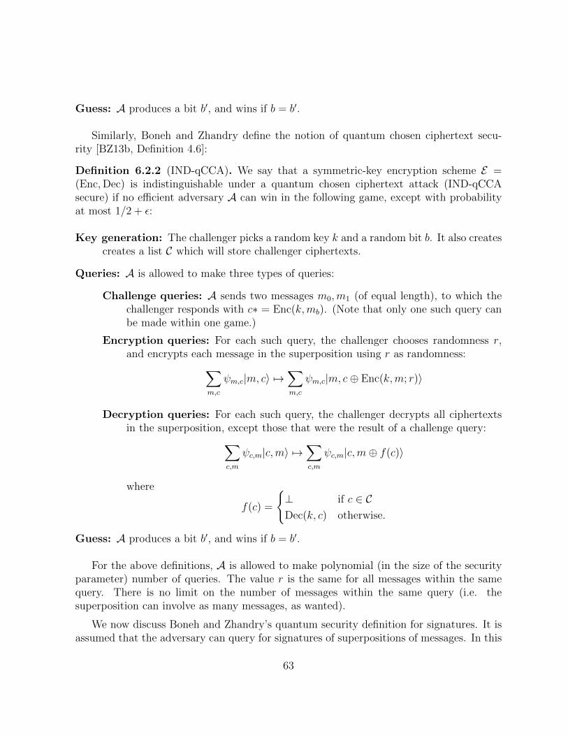
Guess: A produces a bit b′, and wins if b = b′.

Similarly, Boneh and Zhandry define the notion of quantum chosen ciphertext secu-rity [BZ13b, Definition 4.6]:

Definition 6.2.2 (IND-qCCA). We say that a symmetric-key encryption scheme E =(Enc,Dec) is indistinguishable under a quantum chosen ciphertext attack (IND-qCCAsecure) if no efficient adversary A can win in the following game, except with probabilityat most 1/2 + ε:

Key generation: The challenger picks a random key k and a random bit b. It also createscreates a list C which will store challenger ciphertexts.

Queries: A is allowed to make three types of queries:

Challenge queries: A sends two messages m0,m1 (of equal length), to which thechallenger responds with c∗ = Enc(k,mb). (Note that only one such query canbe made within one game.)

Encryption queries: For each such query, the challenger chooses randomness r,and encrypts each message in the superposition using r as randomness:∑

m,c

ψm,c|m, c〉 7→∑m,c

ψm,c|m, c⊕ Enc(k,m; r)〉

Decryption queries: For each such query, the challenger decrypts all ciphertextsin the superposition, except those that were the result of a challenge query:∑

c,m

ψc,m|c,m〉 7→∑c,m

ψc,m|c,m⊕ f(c)〉

where

f(c) =

{⊥ if c ∈ CDec(k, c) otherwise.

Guess: A produces a bit b′, and wins if b = b′.

For the above definitions, A is allowed to make polynomial (in the size of the securityparameter) number of queries. The value r is the same for all messages within the samequery. There is no limit on the number of messages within the same query (i.e. thesuperposition can involve as many messages, as wanted).

We now discuss Boneh and Zhandry’s quantum security definition for signatures. It isassumed that the adversary can query for signatures of superpositions of messages. In this

63

situation, the definition of existential unforgeability needs to be modified, since a naivereading of the definition would allow the adversary simply to measure a superposition andclaim the resulting signature as an existential forgery. Let q be a polynomial function inthe security parameter. For our purposes, the security parameter is the finite field size.To solve this problem we simply require the adversary to produce q + 1 signatures from qqueries [BZ13b, Definition 3.2]:

Definition 6.2.3 (SUF-qCMA). A signature scheme S = (Gen, Sign,Ver) is strongly un-forgeable under a quantum chosen message attack (SUF-qCMA secure) if, for any efficientquantum algorithm A and any polynomial q, the algorithm A’s probability of success inthe following game is negligible in λ:

Key generation: The challenger runs (sk, pk)← Gen(λ), and gives pk to A.

Signing Queries: A makes a polynomial number q of chosen message queries. For eachquery, the challenger chooses randomness r, and responds by signing each messagein the query using r as randomness:∑

m,t

ψm,t|m, t〉 7→∑m,t

ψm,t|m, t⊕ Sign(sk,m; r)〉

Forgeries: A is required to produce q + 1 message-signature pairs. The challenger thenchecks that all the signatures are valid, and that all message-signature pairs aredistinct. If so, the adversary wins.

Definition 6.2.4 (WUF-qCMA). A signature scheme S is weakly unforgeable under aquantum chosen message attack (WUF-qCMA secure) if it satisfies the same definitionas SUF-qCMA, except that we require the q + 1 message-signature pairs to have distinctmessages.

Note that our terminology differs slightly from Boneh and Zhandry [BZ13b], althoughthe content of the definitions is identical: Boneh and Zhandry use the terms “stronglyEUF-qCMA” and “weakly EUF-qCMA” instead of SUF-qCMA and WUF-qCMA. In ad-dition, Boneh and Zhandry have similar definitions for SUF-qCMA and WUF-qCMA securemessage authentication codes [BZ13a].

Finally, we give our definitions of INT-qCTXT and INT-qPTXT. We constructed thesedefinitions by starting with the classical security definitions of INT-CTXT and INT-PTXTfrom Bellare and Namprempre [BN08, §2], and modifying them in a manner similar toBoneh and Zhandry’s definition for digital signatures (Definition 6.2.3).

64

Definition 6.2.5 (INT-qCTXT). An encryption scheme E = (Enc,Dec) satisfies integrityof ciphertext under a quantum attack (INT-qCTXT security) if, for any efficient quantumalgorithm A and any polynomial q, the probability of success of A in the following gameis negligible in λ:

Key generation: The challenger picks a random key k.

Encryption queries: A makes a polynomial q such queries. For each such query, thechallenger chooses randomness r, and encrypts each message in the superpositionusing r as randomness:∑

m,c

ψm,c|m, c〉 7→∑m,c

ψm,c|m, c⊕ Enc(k,m; r)〉

Decryption queries: For each such query, the challenger decrypts all ciphertexts in thesuperposition, except those that were the result of a challenge query:∑

c,m

ψc,m|c,m〉 7→∑c,m

ψc,m|c,m⊕Dec(k, c)〉

Forgeries: A is required to produce q + 1 message-ciphertext pairs. The challenger thenchecks that all the ciphertexts are valid, and that all message-ciphertexts pairs aredistinct. If so, the adversary wins.

Definition 6.2.6 (INT-qPTXT). An encryption scheme E = (Enc,Dec) satisfies the in-tegrity of plaintext under a quantum attack (INT-qPTXT secure) if it satifies the samedefinition as INT-qCTXT, except that we require the q + 1 message-ciphertext pairs tohave distinct messages.

6.3 Main Theorem

In this section, we prove that an IND-qCPA encryption scheme together with a SUF-qCMAsignature or MAC scheme yields an authenticated encryption scheme via the Encrypt-then-MAC method (where the sender first encrypts the message and then signs or produces theMAC for ciphertext), satisfying the respective privacy and integrity guarantees of IND-qCCA (Definition 6.2.2) and INT-qCTXT (Definition 6.2.5), the quantum analogues ofthe classical notions of IND-CCA and INT-CTXT security used in Bellare and Namprem-pre [BN08]. We adopt the proofs to work with the definitions for quantum adversarymodel. We will interchangeably be using Signature and MAC notion as they can replaceeach other. For verification in case of MAC, we simply mean that the party checks and ver-ifies whether or not MAC of the given value is correct. We begin by showing a WUF-qCMAMAC implies INT-qPTXT security:

65

Theorem 6.3.1. Let SE = (Ke, E ,D) be a symmetric-key encryption scheme, letMA = (Km, T ,V) be a message authentication scheme, and let SE = (K, E , D) be theauthenticated encryption scheme obtained from SE and MA via the Encrypt-then-MACmethod. Given any adversary I against SE, we can construct an adversary F such that

AdvINT-qPTXT

SE (I) ≤ AdvWUF-qCMAMA (F ).

Proof. (Based on [BN08, Theorem 4.1]) We construct the adversary F as follows:

1. Use the key Ke.

2. Run I.

3. On query Enc(M) (where M can be in superposition):

C ′ ← E(Ke,M); τ ← Tag(C ′); Return C ′ ‖ τ to I

4. On query Ver(C):

Parse C as C ′ ‖ τ ′; v ← Ver(C ′, τ ′); Return v to I

until I halts.

Let Ci = C ′i ‖ τi for i ∈ {1, . . . , q + 1} be the Ver queries of I that lead to winninggame INT-qPTXTSE , after q queries to Enc. Let Mi = D(Ke, C

′i). We know that due to

the property of INT-qPTXT of SE , at most q of them were obtained from the q queriesto Enc of I; hence C ′is were the result of at most q queries of F to Tag, but we obtainedq + 1 valid tags. Hence, F wins whenever WUF-qCMAMA I wins INT-qPTXTSE .

Although our proof of Theorem 6.3.1 is for MACs, the same proof works for digitalsignatures (replacing the Tag oracle with the Sign oracle). Of course, in the content ofusing signatures, we assume that the public keys are authenticated.

Next we show that a SUF-qCMA signature or MAC implies an INT-qCTXT authenti-cated encryption scheme.

Theorem 6.3.2. Let SE = (Ke, E ,D) be a symmetric-key encryption scheme, letMA = (Km, T ,V) be a message authentication scheme, and let SE = (K, E , D) be the au-thenticated encryption scheme obtained from SE and MA via encrypt-then-MAC compo-sition method. Given any adversary I against SE, we can construct an adversary F suchthat

AdvINT-qCTXT

SE (I) ≤ AdvSUF-qCMAMA (F ).

66

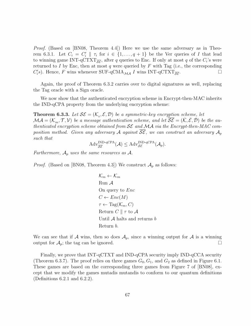
Proof. (Based on [BN08, Theorem 4.4]) Here we use the same adversary as in Theo-rem 6.3.1. Let Ci = C ′i ‖ τi for i ∈ {1, . . . , q + 1} be the Ver queries of I that leadto winning game INT-qCTXTSE , after q queries to Enc. If only at most q of the Ci’s werereturned to I by Enc, then at most q were queried by F with Tag (i.e., the correspondingC ′is). Hence, F wins whenever SUF-qCMAMA I wins INT-qCTXTSE .

Again, the proof of Theorem 6.3.2 carries over to digital signatures as well, replacingthe Tag oracle with a Sign oracle.

We now show that the authenticated encryption scheme in Encrypt-then-MAC inheritsthe IND-qCPA property from the underlying encryption scheme:

Theorem 6.3.3. Let SE = (Ke, E ,D) be a symmetric-key encryption scheme, letMA = (Km, T ,V) be a message authentication scheme, and let SE = (K, E , D) be the au-thenticated encryption scheme obtained from SE andMA via the Encrypt-then-MAC com-position method. Given any adversary A against SE, we can construct an adversary Apsuch that

AdvIND-qCPA

SE (A) ≤ AdvIND-qCPASE (Ap).

Furthermore, Ap uses the same resources as A.

Proof. (Based on [BN08, Theorem 4.3]) We construct Ap as follows:

Km ← KmRun AOn query to Enc

C ← Enc(M)

τ ← Tag(Km, C)

Return C ‖ τ to AUntil A halts and returns b

Return b.

We can see that if A wins, then so does Ap, since a winning output for A is a winningoutput for Ap; the tag can be ignored.

Finally, we prove that INT-qCTXT and IND-qCPA security imply IND-qCCA security(Theorem 6.3.7). The proof relies on three games G0, G1, and G2 as defined in Figure 6.1.These games are based on the corresponding three games from Figure 7 of [BN08], ex-cept that we modify the games mutadis mutandis to conform to our quantum definitions(Definitions 6.2.1 and 6.2.2).

67

Games G0 and G1 : Game G2 :

proc Initialize proc Initialize

K$← K; b

$← {0, 1};S ← ∅ K$← K; b

$← {0, 1}

proc Challenge(M0,M1) proc Challenge(M0,M1)

C$← Enc(K,Mb);S ← S ∪ {C}; Return C C

$← Enc(K,Mb); Return C

proc Enc(M) proc Enc(M)

C$← Enc∗(K,M);S ← S ∪ {C}; Return C C

$← Enc∗(K,M); Return C

proc Dec(C) proc Dec(C)

M ← Dec∗(C) Return ⊥If M 6= ⊥ then bad← true; M ← ⊥Return M

proc Finalize(d) proc Finalize(d)

Return (d = b) Return (d = b)

Figure 6.1: Games G0, G1, and G2.

In figure 6.1 Game G1 contains the code in the box while G0 does not. The functionsEnc∗ and Dec∗ refer to the encryption and decryption oracle functions from Definition 6.2.2.

The proof of Theorem 6.3.7 uses the identical until bad lemma [BN08, Lemma 2.1]:

We first define the term identical until bad using the definition in [BR06], and thenmove on to the lemma.

Definition 6.3.4 (Identical until bad). Games G and H are said to be identical until badif one has the statement if bad then S where the other has the empty statement.

Lemma 6.3.5. (Identical until bad lemma) Let Gi and Gj be identical until bad games,and A an adversary. Then for any y: Pr[GAi =⇒ y]−Pr[GAj =⇒ y] ≤ Pr[Gj sets bad].

It is not immediately clear (to us, anyway) that the identical until bad lemma holds forquantum adversaries. Fortunately, in Theorem 6.3.7, we only need the special case i = 0,j = 1, and y = true, and in this case we can prove the result for quantum adversaries. Weuse the following lemma of Shoup [Sho01, Lemma 1].

68

Lemma 6.3.6. Let E,E ′, and F be events defined on a probability space such that Pr[E∧¬F ] = Pr[E ′ ∧ ¬F ]. Then we have |Pr[E]− Pr[E ′]| ≤ Pr[F ].

This lemma holds regardless of whether or not the adversary is classical or quantum,as it is a mathematical statement. Define the event E to be [GA0 =⇒ true] and E ′ tobe [GA1 =⇒ true]. Define F to be [GA1 sets bad]. Observe that in this case E ∧ ¬Fcorresponds to the outcome M =⊥ in the game G0, meaning that A wins the game.Similarly, E ′ ∧ ¬F corresponds to the outcome M =⊥ in G1, meaning that A wins thegame. Note that for M =⊥, both G0 and G1 return the same responses, and hence havethe same probability of winning. Hence, Pr[E ∧¬F ] = Pr[E ′ ∧¬F ], which means Lemma1 of [Sho01] can be applied to obtain |Pr[E]−Pr[E ′]| ≤ Pr[F ]. Finally, we need to removethe absolute values, to obtain Pr[E ′] ≤ Pr[E]. It is easy to see that we can do so, becausefor G0 we sometimes return the message, while for G1, we always return M = ⊥, so thatthe success probability of G0 is at least that of G1. Hence the identical until bad lemmaholds for quantum adversaries in the special case where i = 0, j = 1, and y = true.

We recall Definition (1) in [BN08]:

AdvIND-CCASE (A) = 2 · Pr[IND-CCAASE =⇒ 1]− 1.

The quantum version of this definition is:

AdvIND-qCCASE (A) = 2 · Pr[IND-qCCAASE =⇒ 1]− 1.

Theorem 6.3.7. Let SE = (K, E ,D) be an encryption scheme. Let A be an IND-qCCAadversary against SE running in time t and making qe Enc queries and qd Dec queries.Then, we can construct an INT-qCTXT adversary Ac and IND-qCPA adversary Ap suchthat

AdvIND-qCCASE (A) ≤ 2 · AdvINT-qCTXT

SE (Ac) + AdvIND-qCPASE (Ap).

Furthermore, Ac runs in time O(t) and makes qe Enc queries and qd Ver queries, while Apruns in time O(t) and makes qe queries of target messages Mi.

Proof. We have:

Pr[IND-qCCAASE =⇒ true] = Pr[GA0 =⇒ true]

= Pr[GA1 =⇒ true]+

(Pr[GA0 =⇒ true]− Pr[GA1 =⇒ true])

≤ Pr[GA1 =⇒ true] + Pr[GA1 sets bad] (6.1)

69

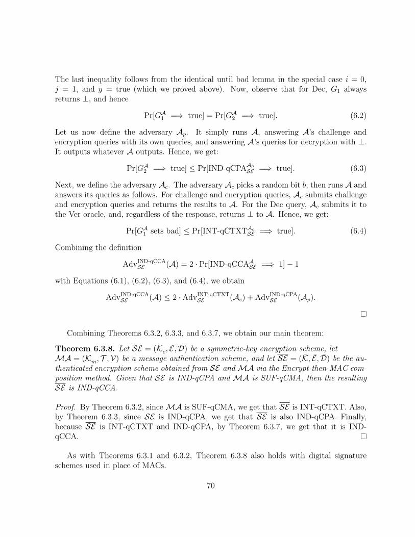
The last inequality follows from the identical until bad lemma in the special case i = 0,j = 1, and y = true (which we proved above). Now, observe that for Dec, G1 alwaysreturns ⊥, and hence

Pr[GA1 =⇒ true] = Pr[GA2 =⇒ true]. (6.2)

Let us now define the adversary Ap. It simply runs A, answering A’s challenge andencryption queries with its own queries, and answering A’s queries for decryption with ⊥.It outputs whatever A outputs. Hence, we get:

Pr[GA2 =⇒ true] ≤ Pr[IND-qCPAApSE =⇒ true]. (6.3)

Next, we define the adversary Ac. The adversary Ac picks a random bit b, then runs A andanswers its queries as follows. For challenge and encryption queries, Ac submits challengeand encryption queries and returns the results to A. For the Dec query, Ac submits it tothe Ver oracle, and, regardless of the response, returns ⊥ to A. Hence, we get:

Pr[GA1 sets bad] ≤ Pr[INT-qCTXTAcSE =⇒ true]. (6.4)

Combining the definition

AdvIND-qCCASE (A) = 2 · Pr[IND-qCCAASE =⇒ 1]− 1

with Equations (6.1), (6.2), (6.3), and (6.4), we obtain

AdvIND-qCCASE (A) ≤ 2 · AdvINT-qCTXT

SE (Ac) + AdvIND-qCPASE (Ap).

Combining Theorems 6.3.2, 6.3.3, and 6.3.7, we obtain our main theorem:

Theorem 6.3.8. Let SE = (Ke, E ,D) be a symmetric-key encryption scheme, letMA = (Km, T ,V) be a message authentication scheme, and let SE = (K, E , D) be the au-thenticated encryption scheme obtained from SE andMA via the Encrypt-then-MAC com-position method. Given that SE is IND-qCPA and MA is SUF-qCMA, then the resultingSE is IND-qCCA.

Proof. By Theorem 6.3.2, sinceMA is SUF-qCMA, we get that SE is INT-qCTXT. Also,by Theorem 6.3.3, since SE is IND-qCPA, we get that SE is also IND-qCPA. Finally,because SE is INT-qCTXT and IND-qCPA, by Theorem 6.3.7, we get that it is IND-qCCA.

As with Theorems 6.3.1 and 6.3.2, Theorem 6.3.8 also holds with digital signatureschemes used in place of MACs.

70

6.4 Quantum-Resistant Strongly Unforgeable Signa-

ture Schemes

In this section we examine some concrete choices of strongly unforgeable signature/MACschemes which could be suitable for our AE construction. We limit ourselves to only a fewrepresentative examples to illustrate the general idea. We focus on signature schemes as inour view they are somewhat more interesting, but similar ideas apply to MACs [BZ13a].We begin with a review of the Boneh-Zhandry transformation [BZ13b, Construction 3.12]for transforming any classically strongly secure digital signature scheme into a SUF-qCMAscheme:

Construction 6.4.1. Let Sc = (Genc, Signc,Verc) be a be a signature scheme, H be a hashfunction, and Q be a family of pairwise independent functions mapping messages to therandomness used by Signc, and k some polynomial in λ. Define S = (Gen, Sign,Ver) where:

• Gen(λ) = Genc(λ)

• Sign(sk,m) :

– Select Q ∈ Q, r ∈ {0, 1}k at random.

– Set s = Q(m), h = H(m, r), σ = Signc(sk, h; s). Output (r, σ).

• Ver(pk,m, (r, σ)) :

– Set h = H(m, r). Output Verc(pk, h, σ).

If the original signature scheme Sc is SUF-CMA against a classical chosen messageattack performed by a quantum adversary, then by [BZ13b, Corollary 3.17] the transformedscheme S is SUF-qCMA in the quantum random oracle model.

Furthermore, if the verification function in the signature scheme Sc involves indepen-dently deriving the value of σ and checking whether or not the derived value matches thevalue which was originally sent, a further optimization is possible: one can hash σ to reduceits length to a minimum. We employ this optimization in our examples.

Note that we have included Q. An example of Q, can be a family of hash functions.We can further assume that whenever needed, we are using this example.

6.4.1 Strong Designated Verifier Signatures from Isogenies

A strong designated verifier signature (SDVS) scheme [JSI96] is a digital signature schemein which only a designated party (specified at the time of signing) can verify signatures, and

71

verification requires that party’s private key. Note that an SDVS is enough for AE, sinceonly the two parties participating in the AE protocol need to be able to verify signatures.

Sun, Tian, and Wang in [STW12] present an isogeny-based SDVS scheme, and givea classical security reduction to the SSDDH problem [JDF11], which is believed to beinfeasible on quantum computers. This reduction qualifies as a straight-line reduction inthe sense of the security framework of Song [Son14], and hence remains valid for quantumadversaries. However, the reduction only establishes SUF-CMA security, not SUF-qCMAsecurity. Applying the Boneh-Zhandry transformation (Construction 6.4.1), we obtain thefollowing SDVS scheme, which is SUF-qCMA:

Setup: Fix a prime p = `eAA `eBB · f ± 1, a supersingular base curve E over Fp2 , generators

{PA, QA} of E[`eAA ], and generators {PB, QB} of E[`eBB ]. Let H1, H2 : {0, 1}∗ → {0, 1}kbe independent secure hash functions (with parameter k), and Q a family of pairwiseindependent functions mapping messages to the randomness used in signing.

Key generation: A signer selects at random mS, nS ∈ Z/`eAA Z, not both divisible by `A,and then computes an isogeny φS : E → ES = E/〈[mS]PA + [nS]QA〉 and the valuesφS(PB) and φS(QB). The private key is (mS, nS) and the public key is the curve ESand the points φS(PB) and φS(QB).A designated verifier selects at random mV , nV ∈ Z/`eBB Z, not both divisible by `B,and then computes an isogeny φV : E → EV = E/〈[mV ]PB + [nV ]QB〉 and the valuesφV (PA) and φV (QA). The private key is (mV , nV ) and the public key is the curve EVand the points φV (PA) and φV (QA).

Signing: Select at random Q ∈ Q, r ∈ {0, 1}k for use in the Boneh-Zhandry transforma-tion. Compute s = Q(m), h = H1(m, r), and φ′S : EV → ESV = EV /〈[mS]φV (PA) +[nS]φV (QA)〉. Set σ = H2(h||j(ESV )||s). The signature is (r, σ).

Verification: Compute φ′V : ES → ESV = ES/〈[mV ]φS(PB) + [nV ]φS(QB)〉 and h =

H1(m, r). Set σ′ = H2(h||j(ESV )||Q(m)). Verify that σ′?= σ.

6.4.2 Ring-LWE Signatures

To give another example, we combine the Ring-LWE signature scheme of Guneysu etal. [GLP15] with Construction 6.4.1 from [BZ13b] to obtain a SUF-qCMA signature schemebased on Ring-LWE:

Setup: Set R = Fq/〈xn + 1〉 where n is a power of 2. Let H1 : {0, 1}∗ → {0, 1}k andH3 : {0, 1}∗ → R be independent secure hash functions (with parameter k) and Q afamily of pairwise independent functions mapping messages to the randomness usedin the signing function. Choose a bound B on the maximum coefficient size.

72

Key generation: A signer generates two small polynomials s1(x), s2(x) ∈ R, selectsa(x) ∈ R at random, and computes the public key t(x) = as1(x) + s2(x).

Signing: Select Q ∈ Q, r ∈ {0, 1}k at random for the Boneh-Zhandry transformation,and y1(x), y2(x) ∈ R at random for the signature scheme. Compute s = Q(m),h = H1(m, r), and c(x) = H3(BitString(a(x)y1(x) + y2(x))||h||s). Finally, computez1(x) = s1(x)c(x) + y1(x) and z2(x) = s2(x)c(x) + y2(x). Check that the coefficientsof the polynomials z1(x), z2(x) are within the bound B; if not, restart. The signatureis (r, z1(x), z2(x), c(x))

Verification: Check that the coefficients of the polynomials z1(x), z2(x) are within the

bound B; if not, reject. Compute x h = H1(m, r), and check whether c(x)?=

H3(a(x)z1(x) + z2(x)− t(x)c(x)||h||Q(m)). If so, accept; otherwise reject.

6.5 Quantum-Resistant Authenticated Encryption

We give a generic construction of authenticated encryption schemes which are provablyquantum-resistant in the sense of INT-qCTXT and IND-qCCA. For the underlying en-cryption scheme, we assume that a classical symmetric-key block cipher E in a suitableblock cipher mode of operation with random IVs will suffice to provide quantum security,taking care to use 2` key sizes to obtain ` bits of security. We refer to [ATTU16] fora discussion of the choice of the mode of operation. For the MAC/signature scheme wecan employ the Boneh-Zhandry transformation on any SUF-CMA scheme secure againstquantum adversaries as described in Section 6.4. Combining those two components, weobtain an IND-qCCA and INT-qCTXT authenticated encryption scheme as follows:

Setup:

1. Choose parameters for the underlying encryption and signature schemes.

2. Let H : {0, 1}∗ → {0, 1}k be a secure hash function (with security parameter k).

3. Let Q be a family of pairwise independent functions mapping messages to therandomness used in the signature scheme.

Key generation:

1. Alice chooses her private parameters for the encryption and signature schemes.If required, she produces and publishes the corresponding public keys.

2. Bob chooses his private parameters for the encryption and signature schemes.If required, he produces and published the corresponding public keys.

73

Encryption:

Suppose Bob wants to send a message m ∈ {0, 1}∗ to Alice.

1. Using the common encryption key e that he shares with Alice, encrypt themessage using the underlying symmetric-key encryption scheme to obtain c =E(e,m).

2. Select Q ∈ Q, r ∈ {0, 1}k at random.

3. Compute t = Q(m).

4. Computes the value h = H(c, r).

5. Using h and his private signing key s, Bob computes the authentication tagσ = Sign(s, h; t).

6. The ciphertext is {c, r, σ}.

Decryption:

Suppose Alice receives ciphertext {c, r, σ} from Bob.

1. Compute the value h = H(c, r).

2. Using h and Bob’s public signing key p, compute the verification functionVer(s, h, r, σ), if it returns true, continue; if not, stop.

3. Using the common encryption key e that she shares with Bob, decrypt themessage and obtain m = D(e, c).

Again, in the case where the verification function in the signature scheme involvesindependently deriving the value of σ and checking that the derived value matches thevalue which was originally sent, we can hash σ prior to transmission to reduce its lengthto a minimum.

6.6 Isogeny-Based Quantum-Resistant Authenticated

Encryption Scheme

In this section, we propose a quantum-resistant authenticated encryption scheme based onisogenies between supersingular elliptic curves. For the key exchange step, we use the pre-vious key exchange scheme of Jao and De Feo from [JDF11] (presented in Chapter 4), andfor the signature scheme, we use the strong designated-verifier scheme from Section 6.4.1.

Setup:

74

1. Choose primes `A, `B, `A′ , `B′ , p, p′ and exponents eA, eB, eA′ , eB′ such that p = `eAA `

eBB ·

f±1 and p′ = `eA′A′ `

eB′B′ ·f ′±1 give us supersingular elliptic curves E/Fp2 (which denote

simply by E) and E/Fp′2 (which denote simply by E ′).

2. Choose bases {PA, QA} and {PB, QB}, which generate E[`eAA ] and E[`eBB ], respectively.

3. Choose bases {PA′ , QA′} and {PB′ , QB′}, which generate E ′[`eA′A′ ] and E ′[`

eB′B′ ], respec-

tively.

4. Let H1, H2 : {0, 1}∗ → {0, 1}k be independent secure hash functions (with parameterk).

Key Generation:

1. Alice chooses random integers mA, nA ∈ Z/`eAA Z not divisible by `A and m′A, n′A ∈

Z/`eA′A′ Z not divisible by `A′ . Then, using these values, computes φA : E → EA =E/〈[mA]PA + [nA]QA〉 and φ′A : E ′ → E ′A = E ′/〈[m′A]PA′ + [n′A]QA′〉. Then, shecomputes φA(PB), φA(QB), φ′A(PB′), φ

′A(QB′) and publishes her public key as:

{EA, E ′A, φA(PB), φA(QB), φ′A(PB′), φ′A(QB′)}.

Her private key is {mA, nA,m′A, n

′A}.

2. Bob chooses random integers mB, nB ∈ Z/`eBB Z not divisible by `B and m′B, n′B ∈

Z/`eB′B′ Z not divisible by `B′ . Then, using these values, computes φB : E → EB =E/〈[mB]PB + [nB]QB〉 and φ′B : E ′ → E ′B = E ′/〈[m′B]PB′ + [n′B]QB′〉. Then, hecomputes φB(PA), φB(QA), φ′B(PA′), φ

′B(QA′) and publishes his public key as:

{EB, E ′B, φB(PA), φB(QA), φ′B(PA′), φ′B(QA′)}.

His private key is {mB, nB,m′B, n

′B}.

Encryption: Suppose Bob wants to send a message m ∈ {0, 1}∗ to Alice.

1. Using Alice’s public parameters {EA, φA(PB), φA(QB)} and his private key, Bob com-putes EAB = EA/〈[mB]φA(PB) + [nB]φA(QB)〉. Then he computes the j-invariant ofEAB, j(EAB).

2. Using the j-invariant and the key to the symmetric encryption scheme, Bob encryptsthe message and obtains c = E(j(EAB),m).

3. Using Alice’s public parameters {E ′A, φ′A(PB′), φ′A(QB′)} and his private key, Bob

computes E ′AB = E ′A/〈[m′B]φ′A(PB′)+[n′B]φ′A(QB′)〉. Then he computes the j-invariantof E ′AB, j(E ′AB).

4. Bob select r ∈ {0, 1}k at random.

75

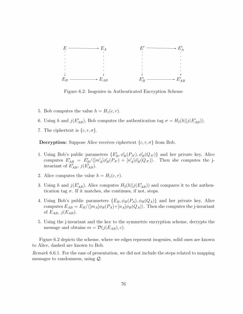
E EA E ′ E ′A

EB EAB E ′B E ′AB

Figure 6.2: Isogenies in Authenticated Encryption Scheme

5. Bob computes the value h = H1(c, r).

6. Using h and j(E ′AB), Bob computes the authentication tag σ = H2(h||j(E ′AB)).

7. The ciphertext is {c, r, σ}.

Decryption: Suppose Alice receives ciphertext {c, r, σ} from Bob.

1. Using Bob’s public parameters {E ′B, φ′B(PA′), φ′B(QA′)} and her private key, Alice

computes E ′AB = E ′B/〈[m′A]φ′B(PA′) + [n′A]φ′B(QA′)〉. Then she computes the j-invariant of E ′AB, j(E ′AB).

2. Alice computes the value h = H1(c, r).

3. Using h and j(E ′AB), Alice computes H2(h||j(E ′AB)) and compares it to the authen-tication tag σ. If it matches, she continues, if not, stops.

4. Using Bob’s public parameters {EB, φB(PA), φB(QA)} and her private key, Alicecomputes EAB = EB/〈[mA]φB(PA)+[nA]φB(QA)〉. Then she computes the j-invariantof EAB, j(EAB).

5. Using the j-invariant and the key to the symmetric encryption scheme, decrypts themessage and obtains m = D(j(EAB), c).

Figure 6.2 depicts the scheme, where we edges represent isogenies, solid ones are knownto Alice, dashed are known to Bob.

Remark 6.6.1. For the ease of presentation, we did not include the steps related to mappingmessages to randomness, using Q.

76

We discuss the security of our scheme. Our scheme uses elliptic curve isogenies in thesame manner as [JDF11]. Thus, under the same security assumptions, namely SSCDH,SSDDH, CSSI, and DSSI, we see that this approach is quantum-secure. For the encryptionpart, we are using a classical symmetric-key encryption scheme, which is believed to beIND-CPA secure against quantum attacks. Assuming that the symmetric-key encryptionscheme is actually secure, we can then achieve IND-qCPA security against quantum ad-versaries (doubling the key size if necessary to fend off quantum brute-force attacks). Aspreviously mentioned, AES is believed to be a suitable such scheme. For the authenti-cation part, we used an SDVS scheme, which we transformed to be SUF-qCMA secure.Finally, by Theorem 6.3.8, we conclude that the resulting scheme is an IND-qCCA andINT-qCTXT secure authenticated encryption scheme.

6.7 Overhead Calculations and Comparisons

In this section we study the communication costs of our AE scheme, from the point of viewof both per-message communication overhead and key transmission overhead.

6.7.1 Communication Overhead

Recall that the ciphertext which Bob sends to Alice consists of the triplet (c, r, σ), wherec is the underlying ciphertext content, r is a k-bit nonce, and σ is the signature tag. Inthe case where the verification function in the signature scheme involves independentlyderiving the value of σ, we can hash σ down to k bits as well. For a security level of `bits, the minimum value of k required for collision resistance is 2` bits in the quantumsetting [Ber09]. The per-message communication overhead of the scheme is thus 4` bits inthe case where the signature tag can be hashed, and 2`+ |σ| bits otherwise. Note that inthe former case the per-message communications overhead is always the same, independentof which component schemes are chosen.

6.7.2 Public Key Overhead

For the overhead involved in transmitting the public keys to be used for the signaturescheme, we use the table of Fujioka et al. [FSXY13], augmented with some more recentresults as described below. Although [FSXY13] deals with the case of post-quantum au-thenticated key exchange, the same key sizes apply to the AE setting.

With the exception of Ring-LWE as explained below, we aim for 128-bit quantumsecurity. For Ring-LWE, we use the numbers from [GLP15]. Since the scheme in [GLP15]

77

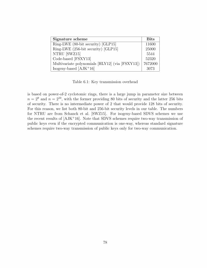
Signature scheme BitsRing-LWE (80-bit security) [GLP15] 11600Ring-LWE (256-bit security) [GLP15] 25000NTRU [SWZ15] 5544Code-based [FSXY13] 52320Multivariate polynomials [HLY12] (via [FSXY13]) 7672000Isogeny-based [AJK+16] 3073

Table 6.1: Key transmission overhead

is based on power-of-2 cyclotomic rings, there is a large jump in parameter size betweenn = 29 and n = 210, with the former providing 80 bits of security and the latter 256 bitsof security. There is no intermediate power of 2 that would provide 128 bits of security.For this reason, we list both 80-bit and 256-bit security levels in our table. The numbersfor NTRU are from Schanck et al. [SWZ15]. For isogeny-based SDVS schemes we usethe recent results of [AJK+16]. Note that SDVS schemes require two-way transmission ofpublic keys even if the encrypted communication is one-way, whereas standard signatureschemes require two-way transmission of public keys only for two-way communication.

78

Chapter 7

Future Work

There are a number of possible directions for further research. Our schemes admit effi-cient implementations in the sense that the running time is polynomial. However, theyare still much slower than traditional schemes such as ECC (which are safe only againstclassical adversaries), as well as certain high-performance quantum-resistant schemes suchas NTRU. There is always a security vs. efficiency trade-off, but we are nevertheless inter-ested in speeding up implementations to the extent that we can. Some low-hanging fruitmay be available in this regard thanks to the existing literature of known optimizationsfor elliptic curve cryptography and elliptic curve arithmetic. For example, existing resultson addition chains could be used to speed up isogeny evaluation.

It is standard in cryptography to cryptanalyze both the details of the proposed protocolsas well as the hardness of the underlying mathematical problem upon which the protocolsare based. Further work in both of these areas is critical in order to build up confidencein the schemes among the wider cryptologic research community.

We seek to construct standard (i.e. non-interactive) digital signature schemes usingisogenies. Such schemes are a fundamental requirement for internet security today. Cur-rently the best we can do is to apply generic transformations which convert interactiveauthentication protocols into non-interactive digital signature schemes. These transforma-tions work, but they are slightly inefficient, introducing a polynomial factor of overheadin both computations and communications. A direct construction of an efficient digitalsignature scheme would be very helpful in order to help make the case for isogeny-basedcryptography.

Another direction is to work on other definitions of security for post-quantum cryptog-raphy. As observed by Boneh and Zhandry in [BZ13b] and by us in Chapter 6, a numberof definitions cannot be directly taken from the classical works and simply used withoutmodification in quantum settings. It is important to review all existing cryptographic secu-

79

rity definitions and analyze whether they are suitable for quantum adversaries, modifyingthem as necessary.

Aside from encryption and digital signatures, the third main pillar of internet securityis authenticated key exchange (AKE). Developing an AKE scheme entails two tasks. First,we need a quantum-aware security model for AKE. Second, we need to develop an actualcandidate for a post-quantum AKE scheme. Our work on authenticated encryption servesas a good foundation for developing security models for AKE.

We have in this thesis laid the initial foundation for post-quantum cryptography basedon supersingular elliptic curve isogenies. This area has great potential and we hope thatthe wider cryptographic community will express an interest and perform more research inthis direction.

80

Bibliography

[AJK+16] Reza Azarderakhsh, David Jao, Kassem Kalach, Brian Koziel, and Christo-pher Leonardi, Key compression for isogeny-based cryptosystems, CryptologyePrint Archive, Report 2016/229, 2016, to appear in AsiaPKC 2016. 78

[AMBGS13] Carlos Aguilar-Melchor, Slim Bettaieb, Philippe Gaborit, and Julien Schrek,A code-based undeniable signature scheme, Cryptography and Coding (Mar-tijn Stam, ed.), Lecture Notes in Computer Science, vol. 8308, Springer BerlinHeidelberg, 2013, pp. 99–119. 49, 59

[ATTU16] Mayuresh Vivekanand Anand, Ehsan Ebrahimi Targhi, Gelo Noel Tabia, andDominique Unruh, Post-quantum security of the CBC, CFB, OFB, CTR, andXTS modes of operation, in Takagi [Tak16], pp. 44–63. 73

[Bac90] Eric Bach, Explicit bounds for primality testing and related problems, Math.Comp. 55 (1990), no. 191, 355–380. 35

[BBBV97] Charles H. Bennett, Ethan Bernstein, Gilles Brassard, and Umesh Vazirani,Strengths and weaknesses of quantum computing, SIAM J. Comput. 26 (1997),1510–1523. 33

[BCL08] Reinier Broker, Denis Xavier Charles, and Kristin Lauter, Evaluating largedegree isogenies and applications to pairing based cryptography, Pairing ’08:Proceedings of the 2nd international conference on Pairing-Based Cryptog-raphy (Berlin, Heidelberg), Springer-Verlag, 2008, pp. 100–112. 24, 25, 30,31

[BCNS14] Joppe W. Bos, Craig Costello, Michael Naehrig, and Douglas Stebila, Post-quantum key exchange for the TLS protocol from the ring learning witherrors problem, Cryptology ePrint Archive, Report 2014/599, 2014, http:

//eprint.iacr.org/. 61

[Bel08] Juliana V. Belding, Number theoretic algorithms for elliptic curves, Ph.D.thesis, University of Maryland, 2008. 47

81

[Ber] Daniel J. Bernstein, How to find smooth parts of integers, URL: http://cr.yp.to/papers.html#smoothparts. Note: draft. 29

[Ber09] Daniel J. Bernstein, Cost analysis of hash collisions: will quantum computersmake SHARCS obsolete?, Workshop Record of SHARCS’09: Special-purposeHardware for Attacking Cryptographic Systems, 2009, pp. 51–82. 77

[Bis11] Gaetan Bisson, Computing endomorphism rings of elliptic curves underthe GRH, Journal of Mathematical Cryptology 5 (2011), no. 2, 101–113,arXiv:1101.4323v2 [math.NT]. 35

[BN08] Mihir Bellare and Chanathip Namprempre, Authenticated encryption: Re-lations among notions and analysis of the generic composition paradigm, J.Cryptol. 21 (2008), no. 4, 469–491. 3, 62, 64, 65, 66, 67, 68, 69

[BR06] Mihir Bellare and Phillip Rogaway, The security of triple encryption and aframework for code-based game-playing proofs, Proceedings of the 24th AnnualInternational Conference on The Theory and Applications of CryptographicTechniques (Berlin, Heidelberg), EUROCRYPT’06, Springer-Verlag, 2006,pp. 409–426. 68

[BS11] Gaetan Bisson and Andrew V. Sutherland, Computing the endomorphism ringof an ordinary elliptic curve over a finite field, Journal of Number Theory 131(2011), no. 5, 815 – 831, Elliptic Curve Cryptography. 25

[BV07] Johannes Buchmann and Ulrich Vollmer, Binary quadratic forms, Algorithmsand Computation in Mathematics, vol. 20, Springer, Berlin, 2007, An algo-rithmic approach. 25, 27, 28, 29, 30, 31, 34

[BZ13a] Dan Boneh and Mark Zhandry, Quantum-secure message authenticationcodes, Advances in Cryptology - EUROCRYPT 2013, 32nd Annual Inter-national Conference on the Theory and Applications of Cryptographic Tech-niques, Athens, Greece, May 26-30, 2013. Proceedings (Thomas Johanssonand Phong Q. Nguyen, eds.), Lecture Notes in Computer Science, vol. 7881,Springer, 2013, pp. 592–608. 64, 71

[BZ13b] Dan Boneh and Mark Zhandry, Secure signatures and chosen ciphertext secu-rity in a quantum computing world, Proc. of Crypto, LNCS, vol. 8043, 2013,pp. 361–379. 62, 63, 64, 71, 72, 79

[CJS14] Andrew M. Childs, David Jao, and Vladimir Soukharev, Constructing ellipticcurve isogenies in quantum subexponential time, J. Mathematical Cryptology8 (2014), no. 1, 1–29. 2, 24, 37, 47

82

[CK01] Ran Canetti and Hugo Krawczyk, Analysis of key-exchange protocols andtheir use for building secure channels, EUROCRYPT (Birgit Pfitzmann, ed.),Lecture Notes in Computer Science, vol. 2045, Springer, 2001, pp. 453–474.48

[CLG09] Denis Xavier Charles, Kristin E. Lauter, and Eyal Z. Goren, Cryptographichash functions from expander graphs, Journal of Cryptology 22 (2009), 93–113. 46

[CM01] Kevin K. H. Cheung and Michele Mosca, Decomposing finite abelian groups,Quantum Inform. Comput. 1 (2001), no. 3, 26–32, arXiv:cs/0101004v1

[cs.DS]. 35

[Cn04] Juan M. Cervino, On the correspondence between supersingular elliptic curvesand maximal quaternionic orders, April 2004, http://arxiv.org/abs/math/0404538. 47

[Cou06] Jean-Marc Couveignes, Hard homogeneous spaces, 2006, http://eprint.

iacr.org/2006/291. 34

[Cox89] David A. Cox, Primes of the form x2 +ny2, A Wiley-Interscience Publication,John Wiley & Sons Inc., New York, 1989, Fermat, class field theory andcomplex multiplication. 16, 17, 19, 26

[DF10] Luca De Feo, Fast algorithms for computing isogenies between ordinary ellipticcurves in small characteristic, Journal of Number Theory 131 (2010), no. 5,873–893. 32

[DFJP14] Luca De Feo, David Jao, and Jerome Plut, Towards quantum-resistant cryp-tosystems from supersingular elliptic curve isogenies, J. Mathematical Cryp-tology 8 (2014), no. 3, 209–247. 3, 37, 49, 55, 59, 60

[DHI02] Wim van Dam, Sean Hallgren, and Lawrence Ip, Quantum algorithms forsome hidden shift problems, SODA ’02: Proceedings of the 14th ACM-SIAMSymposium on Discrete Algorithms, 2002, arXiv:quant-ph/0211140v1,pp. 489–498. 33

[DSV03] Giuliana Davidoff, Peter Sarnak, and Alain Valette, Elementary number the-ory, group theory, and Ramanujan graphs, London Mathematical Society Stu-dent Texts, vol. 55, Cambridge University Press, Cambridge, 2003. 38

[EH00] Mark Ettinger and Peter Høyer, On quantum algorithms for noncommutativehidden subgroups, Advances in Applied Mathematics 25 (2000), 239–251. 33

83

[Eng09] Andreas Enge, Computing modular polynomials in quasi-linear time, Math.Comp. 78 (2009), no. 267, 1809–1824. 25

[FFS88] Uriel Feige, Amos Fiat, and Adi Shamir, Zero-knowledge proofs of identity,Journal of Cryptology 1 (1988), no. 2, 77–94. 56

[Fis14] Dieter Fishbein, Machine-level software optimization of cryptographic proto-cols, Master’s thesis, University of Waterloo, 2014, http://hdl.handle.net/10012/8400. 60

[FM02] Mirelle Fouquet and Francois Morain, Isogeny volcanoes and the SEA algo-rithm, Algorithmic number theory (Sydney, 2002), Lecture Notes in Comput.Sci., vol. 2369, Springer, Berlin, 2002, pp. 276–291. 18, 19

[FSXY13] Atsushi Fujioka, Koutarou Suzuki, Keita Xagawa, and Kazuki Yoneyama,Practical and post-quantum authenticated key exchange from one-way securekey encapsulation mechanism, Proceedings of the 8th ACM SIGSAC Sympo-sium on Information, Computer and Communications Security (New York,NY, USA), ASIA CCS ’13, ACM, 2013, pp. 83–94. 61, 77, 78

[Gal99] Steven D. Galbraith, Constructing isogenies between elliptic curves over finitefields, LMS J. Comput. Math. 2 (1999), 118–138 (electronic). 18, 19, 46, 56

[GHS02] Steven D. Galbraith, Florian Hess, and Nigel P. Smart, Extending the GHSWeil descent attack, Advances in cryptology—EUROCRYPT 2002 (Ams-terdam), Lecture Notes in Comput. Sci., vol. 2332, Springer, Berlin, 2002,pp. 29–44. 25, 37

[GLP15] Tim Guneysu, Vadim Lyubashevsky, and Thomas Poppelmann, Lattice-basedsignatures: Optimization and implementation on reconfigurable hardware,IEEE Trans. Computers 64 (2015), no. 7, 1954–1967. 72, 77, 78

[GMW91] Oded Goldreich, Silvio Micali, and Avi Wigderson, Proofs that yield nothingbut their validity or all languages in NP have zero-knowledge proof systems,Journal of the Association for Computing Machinery 38 (1991), no. 3, 690–728. 40, 48, 56

[GS11] Steven D. Galbraith and Anton Stolbunov, Improved algorithm for the isogenyproblem for ordinary elliptic curves, 2011, http://arxiv.org/abs/1105.

6331/. 37

[HLY12] Yun-Ju Huang, Feng-Hao Liu, and Bo-Yin Yang, Public-key cryptographyfrom new multivariate quadratic assumptions, Public Key Cryptography —

84

PKC 2012 (Marc Fischlin, Johannes Buchmann, and Mark Manulis, eds.),Lecture Notes in Computer Science, vol. 7293, Springer Berlin Heidelberg,2012, pp. 190–205 (English). 78

[HM89] James L. Hafner and Kevin S. McCurley, A rigorous subexponential algorithmfor computation of class groups, J. Amer. Math. Soc. 2 (1989), no. 4, 837–850.25

[IJ10] Sorina Ionica and Antoine Joux, Pairing the volcano, Algorithmic NumberTheory (Guillaume Hanrot, Francois Morain, and Emmanuel Thome, eds.),Lecture Notes in Comput. Sci., vol. 6197, Springer–Verlag, 2010, 9th Interna-tional Symposium, Nancy, France, ANTS-IX, July 19-23, 2010, Proceedings.32

[JDF11] David Jao and Luca De Feo, Towards quantum-resistant cryptosystems fromsupersingular elliptic curve isogenies, PQCrypto (Bo-Yin Yang, ed.), LectureNotes in Computer Science, vol. 7071, Springer, 2011, pp. 19–34. 3, 37, 48,49, 55, 59, 72, 74, 77

[JMV09] David Jao, Stephen D. Miller, and Ramarathnam Venkatesan, Expandergraphs based on GRH with an application to elliptic curve cryptography, J.Number Theory 129 (2009), no. 6, 1491–1504. 26, 27, 38

[JS10] David Jao and Vladimir Soukharev, A subexponential algorithm for evaluatinglarge degree isogenies, Algorithmic number theory, Lecture Notes in Comput.Sci., vol. 6197, Springer, Berlin, 2010, pp. 219–233. 2, 25, 26, 27

[JS14] David Jao and Vladimir Soukharev, Isogeny-based quantum-resistant undeni-able signatures, Post-Quantum Cryptography - 6th International Workshop,PQCrypto 2014, Waterloo, ON, Canada, October 1-3, 2014. Proceedings(Michele Mosca, ed.), Lecture Notes in Computer Science, vol. 8772, Springer,2014, pp. 160–179. 3, 49

[JSI96] Markus Jakobsson, Kazue Sako, and Russell Impagliazzo, Designated verifierproofs and their applications, Advances in Cryptology — EUROCRYPT ’96,International Conference on the Theory and Application of CryptographicTechniques, Saragossa, Spain, May 12-16, 1996, Proceeding (Ueli M. Maurer,ed.), Lecture Notes in Computer Science, vol. 1070, Springer, 1996, pp. 143–154. 71

[KF08] Kaoru Kurosawa and Jun Furukawa, Universally composable undeniable sig-nature, Proceedings of the 35th International Colloquium on Automata, Lan-

85

guages and Programming, Part II (Berlin, Heidelberg), ICALP ’08, Springer-Verlag, 2008, pp. 524–535. 50

[Koh96] David Kohel, Endomorphism rings of elliptic curves over finite fields, Ph.D.thesis, University of California, Berkeley, 1996. 47

[Kup05] Greg Kuperberg, A subexponential-time quantum algorithm for the dihedralhidden subgroup problem, SIAM J. Comput. 35 (2005), no. 1, 170–188. 33,34

[Lan87] Serge Lang, Elliptic functions, second ed., Graduate Texts in Mathematics,vol. 112, Springer-Verlag, New York, 1987, With an appendix by J. Tate. 21

[LPS88] Alexander Lubotzky, Ralph Phillips, and Peter Sarnak, Ramanujan graphs,Combinatorica 8 (1988), no. 3, 261–277. 38

[LS08] Reynald Lercier and Thomas Sirvent, On Elkies subgroups of l-torsion pointsin elliptic curves defined over a finite field, J. Theor. Nombres Bordeaux 20(2008), no. 3, 783–797. 32

[Lub94] Alexander Lubotzky, Discrete groups, expanding graphs and invariant mea-sures, Progress in Mathematics, vol. 125, Birkhauser Verlag, Basel, 1994,With an appendix by Jonathan D. Rogawski. 38

[Mes86] Jean-Francois Mestre, La methode des graphes. Exemples et applications, Pro-ceedings of the international conference on class numbers and fundamentalunits of algebraic number fields (Katata, 1986) (Nagoya), Nagoya Univ., 1986,pp. 217–242. 39

[MOV91] Alfred Menezes, Tatsuaki Okamoto, and Scott Vanstone, Reducing ellipticcurve logarithms to logarithms in a finite field, STOC ’91: Proceedings of thetwenty-third annual ACM symposium on Theory of computing (New York,NY, USA), ACM, 1991, pp. 80–89. 16

[MR14] Diana Maimut and Reza Reyhanitabar, Authenticated encryption: Towardnext-generation algorithms, IEEE Security & Privacy 12 (2014), no. 2, 70–72. 61

[Piz90] Arnold K. Pizer, Ramanujan graphs and Hecke operators, Bull. Amer. Math.Soc. (N.S.) 23 (1990), no. 1, 127–137. 39

[Piz98] Arnold K. Pizer, Ramanujan graphs, Computational perspectives on numbertheory (Chicago, IL, 1995), AMS/IP Stud. Adv. Math., vol. 7, Amer. Math.Soc., Providence, RI, 1998, pp. 159–178. 39

86

[PLQ08] Christophe Petit, Kristin Lauter, and Jean-Jacques Quisquater, Full crypt-analysis of LPS and Morgenstern hash functions, Proceedings of the 6th in-ternational conference on Security and Cryptography for Networks (Berlin,Heidelberg), SCN ’08, Springer-Verlag, 2008, pp. 263–277. 46

[Poi95] David Pointcheval, A new identification scheme based on the perceptrons prob-lem, Advances in Cryptology EUROCRYPT ’95 (Berlin, Heidelberg), Lec-ture Notes in Computer Science, vol. 921, Springer Berlin / Heidelberg, 1995,pp. 319–328. 48

[Reg] Oded Regev, A subexponential time algorithm for the dihedral hidden subgroupproblem with polynomial space, arXiv:quant-ph/0406151v1. 34

[RS06] Alexander Rostovtsev and Anton Stolbunov, Public-key cryptosystem basedon isogenies, 2006, http://eprint.iacr.org/2006/145. 34, 39

[Sar90] Peter Sarnak, Some applications of modular forms, Cambridge Tracts inMathematics, vol. 99, Cambridge University Press, Cambridge, 1990. 38

[Sch91] Arnold Schonhage, Fast reduction and composition of binary quadratic forms,ISSAC ’91: Proceedings of the 1991 international symposium on Symbolicand algebraic computation (New York, NY, USA), ACM, 1991, pp. 128–133.29

[Sch95] Rene Schoof, Counting points on elliptic curves over finite fields, J. Theor.Nombres Bordeaux 7 (1995), no. 1, 219–254, Les Dix-huitiemes JourneesArithmetiques (Bordeaux, 1993). 15, 34

[Sey87] Martin Seysen, A probabilistic factorization algorithm with quadratic formsof negative discriminant, Math. Comp. 48 (1987), no. 178, 757–780. 29

[Sha89] Adi Shamir, An efficient identification scheme based on permuted kernels (ex-tended abstract), Proceedings on Advances in cryptology (New York, NY,USA), CRYPTO ’89, Springer-Verlag New York, Inc., 1989, pp. 606–609. 48

[Sho97] Peter W. Shor, Polynomial-time algorithms for prime factorization and dis-crete logarithms on a quantum computer, SIAM J. Comput. 26 (1997), no. 5,1484–1509, Preliminary version in FOCS ’94. arXiv:quant-ph/9508027v2.1, 34, 35

[Sho01] Victor Shoup, OAEP reconsidered, Advances in Cryptology - CRYPTO 2001,21st Annual International Cryptology Conference, Santa Barbara, California,USA, August 19-23, 2001, Proceedings (Joe Kilian, ed.), Lecture Notes inComputer Science, vol. 2139, Springer, 2001, pp. 239–259. 68, 69

87

[Sil92] Joseph H. Silverman, The arithmetic of elliptic curves, Graduate Texts inMathematics, vol. 106, Springer-Verlag, New York, 1992, Corrected reprintof the 1986 original. 4, 9, 10, 11, 12, 14, 15, 17, 20, 39

[Sil94] Joseph H. Silverman, Advanced topics in the arithmetic of elliptic curves,Graduate Texts in Mathematics, vol. 151, Springer-Verlag, New York, 1994.21

[SJS16] Vladimir Soukharev, David Jao, and Srinath Seshadri, Post-quantum secu-rity models for authenticated encryption, Post-Quantum Cryptography - 7thInternational Workshop, PQCrypto 2016, Fukuoka, Japan, February 24-26,2016, Proceedings, 2016, pp. 64–78. 3, 61

[Son14] Fang Song, A note on quantum security for post-quantum cryptography, Cryp-tology ePrint Archive, Report 2014/709, 2014, http://eprint.iacr.org/.72

[Sou10] Vladimir Soukharev, Evaluating large degree isogenies between elliptic curves,Master’s thesis, University of Waterloo, 2010, http://hdl.handle.net/

10012/5674. 2, 24

[Ste94a] Jacques Stern, Designing identification schemes with keys of short size, Ad-vances in Cryptology CRYPTO ’94 (Berlin, Heidelberg), Lecture Notes inComputer Science, vol. 839, Springer Berlin / Heidelberg, 1994, pp. 164–173.48

[Ste94b] Jacques Stern, A new identification scheme based on syndrome decoding, Ad-vances in Cryptology CRYPTO’ 93 (Berlin, Heidelberg), Lecture Notes inComputer Science, vol. 773, Springer Berlin / Heidelberg, 1994, pp. 13–21.48

[Sto10] Anton Stolbunov, Constructing public-key cryptographic schemes based onclass group action on a set of isogenous elliptic curves, Adv. Math. Commun.4 (2010), no. 2, 215–235. 2, 22, 23, 33, 34, 37, 39, 42, 43, 48

[STW12] Xi Sun, Haibo Tian, and Yumin Wang, Toward quantum-resistant strongdesignated verifier signature from isogenies., INCoS (Fatos Xhafa, LeonardBarolli, Florin Pop, Xiaofeng Chen 0001, and Valentin Cristea, eds.), IEEE,2012, pp. 292–296. 72

[SWZ15] John Schanck, William Whyte, and Zhenfei Zhang, A quantum-safe circuit-extension handshake for tor, Cryptology ePrint Archive, Report 2015/287,2015, http://eprint.iacr.org/. 61, 78

88

[Tak16] Tsuyoshi Takagi (ed.), Post-quantum cryptography - 7th international work-shop, pqcrypto 2016, fukuoka, japan, february 24-26, 2016, proceedings, Lec-ture Notes in Computer Science, vol. 9606, Springer, 2016. 81

[Tan08] Seiichiro Tani, Claw Finding Algorithms Using Quantum Walk, http://

arxiv.org/abs/0708.2584, March 2008. 47

[Tat66] John Tate, Endomorphisms of abelian varieties over finite fields, Invent.Math. 2 (1966), 134–144. 15

[Tes99] Edlyn Teske, The pohlig-hellman method generalized for group structure com-putation, Journal of Symbolic Computation 27 (1999), no. 6, 521–534. 44,47

[Vel71] Jacques Velu, Isogenies entre courbes elliptiques, C. R. Acad. Sci. Paris Ser.A-B 273 (1971), A238–A241. 32

[Wat69] William C. Waterhouse, Abelian varieties over finite fields, Ann. Sci. EcoleNorm. Sup. (4) 2 (1969), 521–560. 21, 22, 33

[Zha05] Shengyu Zhang, Promised and Distributed Quantum Search Computing andCombinatorics, Proceedings of the Eleventh Annual International Confer-ence on Computing and Combinatorics (Berlin, Heidelberg), Lecture Notesin Computer Science, vol. 3595, Springer Berlin / Heidelberg, 2005, pp. 430–439. 47

89