PostgreSQL DevelopmentEssentials

Develop programmatic functions to create powerful databaseapplications

Manpreet KaurBaji Shaik

BIRMINGHAM - MUMBAI

PostgreSQL Development Essentials

Copyright © 2016 Packt Publishing

All rights reserved. No part of this book may be reproduced, stored in a retrieval system, ortransmitted in any form or by any means, without the prior written permission of thepublisher, except in the case of brief quotations embedded in critical articles or reviews.

Every effort has been made in the preparation of this book to ensure the accuracy of theinformation presented. However, the information contained in this book is sold withoutwarranty, either express or implied. Neither the authors, nor Packt Publishing, and itsdealers and distributors will be held liable for any damages caused or alleged to be causeddirectly or indirectly by this book.

Packt Publishing has endeavored to provide trademark information about all of thecompanies and products mentioned in this book by the appropriate use of capitals.However, Packt Publishing cannot guarantee the accuracy of this information.

First published: September 2016

Production reference: 1200916

Published by Packt Publishing Ltd.Livery Place35 Livery StreetBirmingham B3 2PB, UK.

ISBN 978-1-78398-900-3

www.packtpub.com

Credits

Authors Manpreet Kaur Baji Shaik

Copy Editor Zainab Bootwala

Reviewers Daniel Durante Danny Sauer

Project Coordinator Izzat Contractor

Commissioning Editor Julian Ursell

Proofreader Safis Editing

Acquisition Editor Nitin Dasan

Indexer Rekha Nair

Content Development Editor Anish Sukumaran

Graphics Jason Monteiro

Technical Editor Sunith Shetty

Production Coordinator Aparna Bhagat

About the AuthorsManpreet Kaur currently works as a business intelligence solution developer at an IT-basedMNC in Chandigarh. She has over 7 years of work experience in the field of developingsuccessful analytical solutions in data warehousing, analytics and reporting, and portal anddashboard development in the PostgreSQL and Oracle databases. She has worked onbusiness intelligence tools such as Noetix, SSRS, Tableau, and OBIEE. She has a goodunderstanding of ETL tools such as Informatica and Oracle Data Integrator (ODI).Currently, she works on analytical solutions using Hadoop and OBIEE 12c.

Additionally, she is very creative and enjoys oil painting. She also has a youtube channel,Oh so homemade, where she posts easy ways to make recycled crafts.

Baji Shaik is a database administrator and developer. He is currently working as a databaseconsultant at OpenSCG. He has an engineering degree in telecommunications, and hestarted his career as a C# and Java developer. He started working with databases in 2011and, over the years, he has worked with Oracle, PostgreSQL, and Greenplum. Hisbackground spans a wide depth and breadth of expertise and experience in SQL/NoSQLdatabase technologies. He has architectured and designed many successful databasesolutions addressing challenging business requirements. He has provided solutions usingPostgreSQL for reporting, business intelligence, data warehousing, applications, anddevelopment support. He has a good knowledge of automation, orchestration, and DevOpsin a cloud environment.

He comes from a small village named Vutukutu in Andhra Pradesh and currently lives inHyderabad. He likes to watch movies, read books, and write technical blogs. He loves tospend time with family. He has tech-reviewed Troubleshooting PostgreSQL by PacktPublishing. He is a certified PostgreSQL professional.

Thanks to my loving parents. Thanks to Packt Publishing for giving me this opportunity.Special thanks to Izzat Contractor for choosing me, and Anish Sukumaran, Nitin Dasan,and Sunith Shetty for working with me. Thanks to Dinesh Kumar for helping me write.

About the ReviewersDaniel Durante started spending time with computers at the age of 12. He has builtapplications for various sectors, such as the medical industry, universities, themanufacturing industry, and the open source community. He mainly uses Golang, C, Node,or PHP for developing web applications, frameworks, tools, embedded systems, and soon. Some of his personal work can be found on GitHub and his personal website.

He has also worked on the PostgreSQL Developer's Guide, published by Packt Publishing.

I would like to thank my parents, brother, and friends, who’ve all put up with my insanity,day in and day out. I would not be here today if it weren’t for their patience, guidance, andlove.

Danny Sauer has been a Linux sysadmin, software developer, security engineer, opensource advocate, and general computer geek at various companies for around 20 years. Hehas administered, used, and programmed PostgreSQL for over half of that time. When he'snot building solutions in the digital world, he and his wife enjoy restoring their antiquehome and teaching old cars new tricks.

www.PacktPub.comeBooks, discount offers, and moreDid you know that Packt offers eBook versions of every book published, with PDF andePub files available? You can upgrade to the eBook version at www.PacktPub.com and as aprint book customer, you are entitled to a discount on the eBook copy. Get in touch with usat customercare@packtpub.com for more details.

At www.PacktPub.com, you can also read a collection of free technical articles, sign up for arange of free newsletters and receive exclusive discounts and offers on Packt books andeBooks.

h t t p s : / / w w w 2 . p a c k t p u b . c o m / b o o k s / s u b s c r i p t i o n / p a c k t l i b

Do you need instant solutions to your IT questions? PacktLib is Packt's online digital booklibrary. Here, you can search, access, and read Packt's entire library of books.

Why subscribe?Fully searchable across every book published by PacktCopy and paste, print, and bookmark contentOn demand and accessible via a web browser

Table of ContentsPreface 1

Chapter 1: Advanced SQL 5

Creating views 5Deleting and replacing views 7

Materialized views 8Why materialized views? 8

Read-only, updatable, and writeable materialized views 8Read-only materialized views 9Updatable materialized views 9Writeable materialized views 10

Creating cursors 10Using cursors 11Closing a cursor 12

Using the GROUP BY clause 12Using the HAVING clause 14

Parameters or arguments 14Using the UPDATE operation clauses 15Using the LIMIT clause 15Using subqueries 16Subqueries that return multiple rows 18

Correlated subqueries 18Existence subqueries 19Parameters or arguments 19

Using the Union join 20Using the Self join 21Using the Outer join 22

Left outer join 23Right outer join 24Full outer join 24

Summary 26

Chapter 2: Data Manipulation 27

Conversion between datatypes 27Introduction to arrays 28

Array constructors 28

[ ii ]

String_to_array() 31Array_dims( ) 32ARRAY_AGG() 32ARRAY_UPPER() 34Array_length() 34

Array slicing and splicing 34UNNESTing arrays to rows 35Introduction to JSON 37

Inserting JSON data in PostgreSQL 37Querying JSON 38

Equality operation 38Containment 38Key/element existence 39Outputting JSON 40

Using XML in PostgreSQL 41Inserting XML data in PostgreSQL 41

Querying XML data 42Composite datatype 42

Creating composite types in PostgreSQL 42Altering composite types in PostgreSQL 44Dropping composite types in PostgreSQL 45

Summary 45

Chapter 3: Triggers 46

Introduction to triggers 46Adding triggers to PostgreSQL 47Modifying triggers in PostgreSQL 52Removing a trigger function 53

Creating a trigger function 54Testing the trigger function 55Viewing existing triggers 56

Summary 57

Chapter 4: Understanding Database Design Concepts 58

Basic design rules 58The ability to solve the problem 58The ability to hold the required data 59The ability to support relationships 59The ability to impose data integrity 59The ability to impose data efficiency 59The ability to accommodate future changes 59

Normalization 60Anomalies in DBMS 60

[ iii ]

First normal form 62Second normal form 62Third normal form 63Common patterns 64

Many-to-many relationships 64Hierarchy 65Recursive relationships 66

Summary 67

Chapter 5: Transactions and Locking 68

Defining transactions 68ACID rules 69Effect of concurrency on transactions 70Transactions and savepoints 70Transaction isolation 71

Implementing isolation levels 72Dirty reads 72Non-repeatable reads 73Phantom reads 74

ANSI isolation levels 74Transaction isolation levels 75Changing the isolation level 75Using explicit and implicit transactions 76

Avoiding deadlocks 76Explicit locking 77

Locking rows 77Locking tables 78

Summary 79

Chapter 6: Indexes and Constraints 81

Introduction to indexes and constraints 81Primary key indexes 82Unique indexes 83B-tree indexes 84Standard indexes 85Full text indexes 86Partial indexes 86Multicolumn indexes 88Hash indexes 89GIN and GiST indexes 89

Clustering on an index 90Foreign key constraints 91

[ iv ]

Unique constraints 92Check constraints 94NOT NULL constraints 95

Exclusion constraints 96Summary 96

Chapter 7: Table Partitioning 97

Table partitioning 97Partition implementation 102Partitioning types 107

List partition 107Managing partitions 109Adding a new partition 109Purging an old partition 110Alternate partitioning methods 111

Method 1 111Method 2 112

Constraint exclusion 114Horizontal partitioning 116PL/Proxy 117Foreign inheritance 118

Summary 121

Chapter 8: Query Tuning and Optimization 122

Query tuning 122Hot versus cold cache 123Cleaning the cache 124

pg_buffercache 127pg_prewarm 129

Optimizer settings for cached data 130Multiple ways to implement a query 132Bad query performance with stale statistics 134

Optimizer hints 136Explain Plan 141

Generating and reading the Explain Plan 141Simple example 142More complex example 142

Query operators 143Seq Scan 143Index Scan 143Sort 144Unique 144

[ v ]

LIMIT 144Aggregate 144Append 144Result 144Nested Loop 145Merge Join 145Hash and Hash Join 145Group 145Subquery Scan and Subplan 145Tid Scan 145Materialize 146Setop 146

Summary 146

Chapter 9: PostgreSQL Extensions and Large Object Support 147

Creating an extension 147Compiling extensions 149Database links in PostgreSQL 150

Using binary large objects 153Creating a large object 154Importing a large object 154Exporting a large object 155Writing data to a large object 155Server-side functions 155

Summary 156

Chapter 10: Using PHP in PostgreSQL 157

Postgres with PHP 157PHP-to-PostgreSQL connections 158Dealing with DDLs 161DML operations 162

pg_query_params 163pg_insert 164

Data retrieval 165pg_fetch_all 165pg_fetch_assoc 166pg_fetch_result 167

Helper functions to deal with data fetching 168pg_free_results 168pg_num_rows 168

[ vi ]

pg_num_fields 168pg_field_name 168pg_meta_data 168pg_convert 169UPDATE 171DELETE 172COPY 172

Summary 174

Chapter 11: Using Java in PostgreSQL 175

Making database connections to PostgreSQL using Java 175Using Java to create a PostgreSQL table 178Using Java to insert records into a PostgreSQL table 179Using Java to update records into a PostgreSQL table 180Using Java to delete records into a PostgreSQL table 181Catching exceptions 182

Using prepared statements 184Loading data using COPY 184

Connection properties 186Summary 187

Index 188

PrefaceThe purpose of this book is to teach you the fundamental practices and techniques ofdatabase developers for programming database applications with PostgreSQL. It is targetedto database developers using PostgreSQL who have basic experience developing databaseapplications with the system, but want a deeper understanding of how to implementprogrammatic functions with PostgreSQL.

What this book coversChapter 1, Advanced SQL, aims to help you understand advanced SQL topics such as views,materialized views, and cursors and will be able to get a sound understanding of complextopics such as subqueries and joins.

Chapter 2, Data Manipulation, provides you the ability to perform data type conversionsand perform JSON and XML operations in PostgreSQL.

Chapter 3, Triggers, explains how to perform trigger operations and use trigger functions inPostgreSQL.

Chapter 4, Understanding Database Design Concepts, explains data modeling andnormalization concepts. The reader will then be able to efficiently create a robust databasedesign.

Chapter 5, Transactions and Locking, covers the effect of transactions and locking on thedatabase.The reader will also be able to understand isolation levels and understand multi-version concurrency control behavior.

Chapter 6, Indexes And Constraints, provides knowledge about the different indexes andconstraints available in PostgreSQL. This knowledge will help the reader while coding andthe reader will be in a better position to choose among the different indexes and constraintsdepending upon the requirement during the coding phase.

Chapter 7, Table Partitioning, gives the reader a better understanding of partitioning inPostgreSQL. The reader will be able to use the different partitioning methods available inPostgreSQL and also implement horizontal partitioning using PL/Proxy.

Preface

[ 2 ]

Chapter 8, Query Tuning and Optimization, provides knowledge about different mechanismsand approaches available to tune a query. The reader will be able to utilize this knowledgein order to write a optimal/efficient query or code.

Chapter 9, PostgreSQL Extensions and Large Object Support, will familiarize the reader withthe concept of extensions in PostgreSQL and also with the usage of large objects' datatypesin PostgreSQL.

Chapter 10, Using PHP in PostgreSQL, covers the basics of performing database operationsin PostgreSQL using the PHP language, which helps reader to start with PHP code.

Chapter 11, Using Java in PostgreSQL, this chapter provides knowledge about databaseconnectivity using Java and creating/modifying objects using Java code. It also talks aboutJDBC drivers.

What you need for this bookYou need PostgreSQL 9.4 or higher to be installed on your machine to test the codesprovided in the book. As this covers Java and PHP, you need Java and PHP binariesinstalled on your machine. All other tools covered in this book have installation proceduresincluded, so there's no need to install them before you start reading the book.

Who this book is forThis book is mainly for PostgreSQL developers who want to develop applications usingprogramming languages. It is also useful for tuning databases through query optimization,indexing, and partitioning.

ConventionsIn this book, you will find a number of text styles that distinguish between different kindsof information. Here are some examples of these styles and an explanation of their meaning.

Code words in text, database table names, folder names, filenames, file extensions,pathnames, dummy URLs, user input, and Twitter handles are shown as follows: "Databaseviews are created using the CREATE VIEW statement. "

Preface

[ 3 ]

A block of code is set as follows:

import java.sql.Connection;import java.sql.DriverManager;import java.sql.Statement;import java.sql.ResultSet;import java.sql.SQLException;

Any command-line input or output is written as follows:

CREATE VIEW view_name ASSELECT column1, column2FROM table_nameWHERE [condition];

New terms and important words are shown in bold.

Warnings or important notes appear in a box like this.

Tips and tricks appear like this.

Reader feedbackFeedback from our readers is always welcome. Let us know what you think about thisbook—what you liked or disliked. Reader feedback is important for us as it helps usdevelop titles that you will really get the most out of. To send us general feedback, simplye-mail feedback@packtpub.com, and mention the book's title in the subject of yourmessage. If there is a topic that you have expertise in and you are interested in eitherwriting or contributing to a book, see our author guide at www.packtpub.com/authors.

Customer supportNow that you are the proud owner of a Packt book, we have a number of things to help youto get the most from your purchase.

Preface

[ 4 ]

ErrataAlthough we have taken every care to ensure the accuracy of our content, mistakes dohappen. If you find a mistake in one of our books-maybe a mistake in the text or the code-we would be grateful if you could report this to us. By doing so, you can save other readersfrom frustration and help us improve subsequent versions of this book. If you find anyerrata, please report them by visiting h t t p : / / w w w . p a c k t p u b . c o m / s u b m i t - e r r a t a, selectingyour book, clicking on the Errata Submission Form link, and entering the details of yourerrata. Once your errata are verified, your submission will be accepted and the errata willbe uploaded to our website or added to any list of existing errata under the Errata section ofthat title.

To view the previously submitted errata, go to h t t p s : / / w w w . p a c k t p u b . c o m / b o o k s / c o n t e n

t / s u p p o r t and enter the name of the book in the search field. The required information willappear under the Errata section.

PiracyPiracy of copyrighted material on the Internet is an ongoing problem across all media. AtPackt, we take the protection of our copyright and licenses very seriously. If you comeacross any illegal copies of our works in any form on the Internet, please provide us withthe location address or website name immediately so that we can pursue a remedy.

Please contact us at copyright@packtpub.com with a link to the suspected piratedmaterial.

We appreciate your help in protecting our authors and our ability to bring you valuablecontent.

QuestionsIf you have a problem with any aspect of this book, you can contact usat questions@packtpub.com, and we will do our best to address the problem.

1Advanced SQL

This book is all about an open source software product, a relational database calledPostgreSQL. PostgreSQL is an advanced SQL database server, available on a wide range ofplatforms. The purpose of this book is to teach database developers the fundamentalpractices and techniques to program database applications with PostgreSQL.

In this chapter, we will discuss the following advanced SQL topics:

Creating viewsUnderstanding materialized viewsCreating cursorsUsing the GROUP BY clauseUsing the HAVING clauseUnderstanding complex topics such as subqueries and joins

Creating viewsA view is a virtual table based on the result set of an SQL statement. Just like a real table, aview consist of rows and columns. The fields in a view are from one or more real tables inthe database. Generally speaking, a table has a set of definitions that physically stores data.A view also has a set of definitions built on top of table(s) or other view(s) that does notphysically store data. The purpose of creating views is to make sure that the user does nothave access to all the data and is being restricted through a view. Also, it's better to create a view if we have a query based on multiple tables so that we can use it straightaway ratherthan writing a whole PSQL again and again.

Database views are created using the CREATE VIEW statement. Views can be created from asingle table or multiple tables, or another view.

Advanced SQL

[ 6 ]

The basic CREATEVIEW syntax is as follows:

CREATE VIEW view_name ASSELECT column1, column2FROM table_nameWHERE [condition];

Let's take a look at each of these commands:

CREATE VIEW: This command helps create the database's view.SELECT: This command helps you select the physical and virtual columns thatyou want as part of the view.FROM: This command gives the table names with an alias from where we can fetchthe columns. This may include one or more table names, considering you have tocreate a view at the top of multiple tables.WHERE: This command provides a condition that will restrict the data for a view.Also, if you include multiple tables in the FROM clause, you can provide thejoining condition under the WHERE clause.

You can then query this view as though it were a table. (In PostgreSQL, at the time ofwriting, views are read-only by default.) You can SELECT data from a view just as youwould from a table and join it to other tables; you can also use WHERE clauses. Each timeyou execute a SELECT query using the view, the data is rebuilt, so it is always up-to-date. Itis not a frozen copy stored at the time the view was created.

Let's create a view on supplier and order tables. But, before that, let's see what the structureof the suppliers and orders table is:

CREATE TABLE suppliers(supplier_id number primary key,Supplier_name varchar(30),Phone_number number);CREATE TABLE orders(order_number number primary key,Supplier_id number references suppliers(supplier_id),Quanity number,Is_active varchar(10),Price number);CREATE VIEW active_supplier_orders ASSELECT suppliers.supplier_id, suppliers.supplier_name orders.quantity,orders.priceFROM suppliersINNER JOIN ordersON suppliers.supplier_id = orders.supplier_idWHERE suppliers.supplier_name = 'XYZ COMPANY'

Advanced SQL

[ 7 ]

And orders.active='TRUE';

The preceding example will create a virtual table based on the result set of the SELECTstatement. You can now query the PostgreSQL VIEW as follows:

SELECT * FROM active_supplier_orders;

Deleting and replacing viewsTo delete a view, simply use the DROP VIEW statement with view_name. The basicDROPVIEW syntax is as follows:

DROP VIEW IF EXISTS view_name;

If you want to replace an existing view with one that has the same name and returns thesame set of columns, you can use a CREATE OR REPLACE command.

The following is the syntax to modify an existing view:

CREATE OR REPLACE VIEW view_name ASSELECT column_name(s)FROM table_name(s)WHERE condition;

Let's take a look at each of these commands:

CREATE OR REPLACE VIEW: This command helps modify the existing view.SELECT: This command selects the columns that you want as part of the view.FROM: This command gives the table name from where we can fetch the columns.This may include one or more table names, since you have to create a view at thetop of multiple tables.WHERE: This command provides the condition to restrict the data for a view. Also,if you include multiple tables in the FROM clause, you can provide the joiningcondition under the WHERE clause.

Let's modify a view, supplier_orders, by adding some more columns in the view. Theview was originally based on supplier and order tables having supplier_id,supplier_name, quantity, and price. Let's also add order_number in the view.

CREATE OR REPLACE VIEW active_supplier_orders ASSELECT suppliers.supplier_id, suppliers.supplier_name orders.quantity,orders.price,order. order_numberFROM suppliers

Advanced SQL

[ 8 ]

INNER JOIN ordersON suppliers.supplier_id = orders.supplier_idWHERE suppliers.supplier_name = 'XYZ COMPANY'And orders.active='TRUE';;

Materialized viewsA materialized view is a table that actually contains rows but behaves like a view. This hasbeen added in the PostgreSQL 9.3 version. A materialized view cannot subsequently bedirectly updated, and the query used to create the materialized view is stored in exactly thesame way as the view's query is stored. As it holds the actual data, it occupies space as perthe filters that we applied while creating the materialized view.

Why materialized views?Before we get too deep into how to implement materialized views, let's first examine whywe may want to use materialized views.

You may notice that certain queries are very slow. You may have exhausted all thetechniques in the standard bag of techniques to speed up those queries. In the end, you willrealize that getting queries to run as fast as you want simply isn't possible withoutcompletely restructuring the data.

Now, if you have an environment where you run the same type of SELECT query multipletimes against the same set of tables, then you can create a materialized view for SELECT sothat, on every run, this view does not go to the actual tables to fetch the data, which willobviously reduce the load on them as you might be running a Data ManipulationLanguage (DML) against your actual tables at the same time. So, basically, you take a viewand turn it into a real table that holds real data rather than a gateway to a SELECT query.

Read-only, updatable, and writeable materialized viewsA materialized view can be read-only, updatable, or writeable. Users cannot perform DMLstatements on read-only materialized views, but they can perform them on updatable andwriteable materialized views.

Advanced SQL

[ 9 ]

Read-only materialized viewsYou can make a materialized view read-only during creation by omitting the FOR UPDATEclause or by disabling the equivalent option in the database management tool. Read-onlymaterialized views use many mechanisms similar to updatable materialized views, exceptthey do not need to belong to a materialized view group.

In a replication environment, a materialized table holds the table data and resides in adifferent database. A table that has a materialized view on it is called a master table. Themaster table resides on a master site and the materialized view resides on a materialized-view site.

In addition, using read-only materialized views eliminates the possibility of introducingdata conflicts on the master site or the master materialized view site, although thisconvenience means that updates cannot be made on the remote materialized view site.

The syntax to create a materialized view is as follows:

CREATE MATERIALIZED VIEW view_name AS SELECT columns FROM table;

The CREATE MATERIALIZED VIEW command helps us create a materialized view. Thecommand acts in way similar to the CREATE VIEW command, which was explained in theprevious section.

Let's make a read-only materialized view for a supplier table:

CREATE MATERIALIZED VIEW suppliers_matview ASSELECT * FROM suppliers;

This view is a read-only materialized view and will not reflect the changes to the mastersite.

Updatable materialized viewsYou can make a materialized view updatable during creation by including the FOR UPDATEclause or enabling the equivalent option in the database management tool. In order forchanges that have been made to an updatable materialized view to be reflected in themaster site during refresh, the updatable materialized view must belong to a materializedview group.

When we say “refreshing the materialized view,” we mean synchronizing the data in thematerialized view with data in its master table.

Advanced SQL

[ 10 ]

An updatable materialized view enables you to decrease the load on master sites becauseusers can make changes to data on the materialized view site.

The syntax to create an updatable materialized view is as follows:

CREATE MATERIALIZED VIEW view_name FOR UPDATEASSELECT columns FROM table;

Let's make an updatable materialized view for a supplier table:

CREATE MATERIALIZED VIEW suppliers_matview FOR UPDATEASSELECT * FROM suppliers;

Whenever changes are made in the suppliers_matview clause, it will reflect the changesto the master sites during refresh.

Writeable materialized viewsA writeable materialized view is one that is created using the FOR UPDATE clause like anupdatable materialized view is, but it is not a part of a materialized view group. Users canperform DML operations on a writeable materialized view; however, if you refresh thematerialized view, then these changes are not pushed back to the master site and are lost inthe materialized view itself. Writeable materialized views are typically allowed whereverfast-refreshable, read-only materialized views are allowed.

Creating cursorsA cursor in PostgreSQL is a read-only pointer to a fully executed SELECT statement's resultset. Cursors are typically used within applications that maintain a persistent connection tothe PostgreSQL backend. By executing a cursor and maintaining a reference to its returnedresult set, an application can more efficiently manage which rows to retrieve from a resultset at different times without re-executing the query with different LIMIT and OFFSETclauses.

The four SQL commands involved with PostgreSQL cursors are DECLARE, FETCH, MOVE, andCLOSE.

Advanced SQL

[ 11 ]

The DECLARE command both defines and opens a cursor, in effect defining the cursor inmemory, and then populates the cursor with information about the result set returned fromthe executed query. A cursor may be declared only within an existing transaction block, soyou must execute a BEGIN command prior to declaring a cursor.

Here is the syntax for DECLARE:

DECLARE cursorname [ BINARY ] [ INSENSITIVE ] [ SCROLL ] CURSOR FOR query[ FOR { READ ONLY | UPDATE [ OF column [, ...] ] } ]

DECLARE cursorname is the name of the cursor to create. The optional BINARY keywordcauses the output to be retrieved in binary format instead of standard ASCII; this can bemore efficient, though it is only relevant to custom applications as clients such as psql arenot built to handle anything but text output. The INSENSITIVE and SCROLL keywords existto comply with the SQL standard, though they each define PostgreSQL's default behaviorand are never necessary. The INSENSITIVE SQL keyword exists to ensure that all dataretrieved from the cursor remains unchanged from other cursors or connections. AsPostgreSQL requires the cursors to be defined within transaction blocks, this behavior isalready implied. The SCROLL SQL keyword exists to specify that multiple rows at a timecan be selected from the cursor. This is the default in PostgreSQL, even if it is unspecified.

The CURSOR FOR query is the complete query and its result set will be accessible by thecursor when executed.

The [FOR { READ ONLY | UPDATE [ OF column [, ...] ] } ] cursors may only bedefined as READ ONLY, and the FOR clause is, therefore, superfluous.

Let's begin a transaction block with the BEGIN keyword, and open a cursor namedorder_cur with SELECT * FROM orders as its executed select statement:

BEGIN;DECLARE order_cur CURSORFOR SELECT * FROM orders;

Once the cursor is successfully declared, it means that the rows retrieved by the query arenow accessible from the order_cur cursor.

Using cursorsIn order to retrieve rows from the open cursor, we need to use the FETCH command. TheMOVE command moves the current location of the cursor within the result set and the CLOSEcommand closes the cursor, freeing up any associated memory.

Advanced SQL

[ 12 ]

Here is the syntax for the FETCH SQL command:

FETCH [ FORWARD | BACKWARD][ # | ALL | NEXT | PRIOR ]{ IN | FROM }cursor

cursor is the name of the cursor from where we can retrieve row data. A cursor alwayspoints to a current position in the executed statement's result set and rows can be retrievedeither ahead of the current location or behind it. The FORWARD and BACKWARD keywordsmay be used to specify the direction, though the default is forward. The NEXT keyword (thedefault) returns the next single row from the current cursor position. The PRIOR keywordcauses the single row preceding the current cursor position to be returned.

Let's consider an example that fetches the first four rows stored in the result set, pointed toby the order_cur cursor. As a direction is not specified, FORWARD is implied. It then uses aFETCH statement with the NEXT keyword to select the fifth row, and then another FETCHstatement with the PRIOR keyword to again select the fourth retrieved row.

FETCH 4 FROM order_cur;

In this case, the first four rows will be fetched.

Closing a cursorYou can use the CLOSE command to explicitly close an open cursor. A cursor can also beimplicitly closed if the transaction block that it resides within is committed with the COMMITcommand, or rolled back with the ROLLBACK command.

Here is the syntax for the CLOSE command, where Cursorname is the name of the cursorintended to be closed:

CLOSECursorname;

Using the GROUP BY clauseThe GROUP BY clause enables you to establish data groups based on columns. The groupingcriterion is defined by the GROUP BY clause, which is followed by the WHERE clause in theSQL execution path. Following this execution path, the result set rows are grouped basedon like values of grouping columns and the WHERE clause restricts the entries in each group.

Advanced SQL

[ 13 ]

All columns that are used besides the aggregate functions must beincluded in the GROUP BY clause. The GROUP BY clause does not supportthe use of column aliases; you must use the actual column names. TheGROUP BY columns may or may not appear in the SELECT list. The GROUPBY clause can only be used with aggregate functions such as SUM, AVG,COUNT, MAX, and MIN.

The following statement illustrates the syntax of the GROUP BY clause:

SELECT expression1, expression2, ... expression_n,aggregate_function (expression)FROM tablesWHERE conditionsGROUP BY expression1, expression2, ... expression_n;

The expression1, expression2, ... expression_n commands are expressions thatare not encapsulated within an aggregate function and must be included in the GROUP BYclause.

Let's take a look at these commands:

aggregate_function: This performs many functions, such as SUM ( h t t p : / / w w w

. t e c h o n t h e n e t . c o m / o r a c l e / f u n c t i o n s / s u m . p h p), COUNT ( h t t p : / / w w w . t e c h o n t

h e n e t . c o m / o r a c l e / f u n c t i o n s / c o u n t . p h p), MIN ( h t t p : / / w w w . t e c h o n t h e n e t . c o

m / o r a c l e / f u n c t i o n s / m i n . p h p), MAX ( h t t p : / / w w w . t e c h o n t h e n e t . c o m / o r a c l e / f

u n c t i o n s / m a x . p h p), or AVG ( h t t p : / / w w w . t e c h o n t h e n e t . c o m / o r a c l e / f u n c t i o n

s / a v g . p h p).tables: This is where you can retrieve records from. There must be at least onetable listed in the FROM clause.conditions: This is a condition that must be met for the records to be selected.

The GROUP BY clause must appear right after the FROM or WHERE clause. Followed by theGROUP BY clause is one column or a list of comma-separated columns. You can also put anexpression in the GROUP BY clause.

As mentioned in the previous paragraph, the GROUP BY clause divides rows returned fromthe SELECT statement into groups. For each group, you can apply an aggregate function,for example, to calculate the sum of items or count the number of items in the groups.

Advanced SQL

[ 14 ]

Let's look at a GROUP BY query example that uses the SUM function ( h t t p : / / w w w . t e c h o n t h e

n e t . c o m / o r a c l e / f u n c t i o n s / s u m . p h p). This example uses the SUM function to return thename of the product and the total sales (for the product).

SELECT product, SUM(sale) AS "Total sales"FROM order_detailsGROUP BY product;

In the select statement, we have sales where we applied the SUM function and the other fieldproduct is not part of SUM, we must use in the GROUP BY clause.

Using the HAVING clauseIn the previous section, we discussed about GROUP BY clause, however if you want torestrict the groups of returned rows, you can use HAVING clause. The HAVING clause is usedto specify which individual group(s) is to be displayed, or in simple language we use theHAVING clause in order to filter the groups on the basis of an aggregate function condition.

Note: The WHERE clause cannot be used to return the desired groups. The WHERE clause isonly used to restrict individual rows. When the GROUP BY clause is not used, the HAVINGclause works like the WHERE clause.

The syntax for the PostgreSQL HAVING clause is as follows:

SELECT expression1, expression2, ... expression_n,aggregate_function (expression)FROM tablesWHERE conditionsGROUP BY expression1, expression2, ... expression_nHAVING group_condition;

Parameters or argumentsaggregate_function can be a function such as SUM, COUNT, MIN, MAX, or AVG.

expression1, expression2, ... expression_n are expressions that are notencapsulated within an aggregate function and must be included in the GROUP BY clause.

conditions are the conditions used to restrict the groups of returned rows. Only thosegroups whose condition evaluates to true will be included in the result set.

Advanced SQL

[ 15 ]

Let's consider an example where you try to fetch the product that has sales>10000:

SELECT product, SUM(sale) AS "Total sales"FROM order_detailsGROUP BY productHaving sum(sales)>10000;

The PostgreSQL HAVING clause will filter the results so that only the total sales greater than10000 will be returned.

Using the UPDATE operation clausesThe PostgreSQL UPDATE query is used to modify the existing records in a table. You can usethe WHERE clause with the UPDATE query to update selected rows; otherwise, all the rowswill be updated.

The basic syntax of the UPDATE query with the WHERE clause is as follows:

UPDATE table_nameSET column1 = value1, column2 = value2...., columnN = valueNWHERE [condition];

You can combine n number of conditions using the AND or OR operators.

The following is an example that will update SALARY for an employee whose ID is 6:

UPDATE employee SET SALARY = 15000 WHERE ID = 6;

This will update the salary to 15000 whose ID = 6.

Using the LIMIT clauseThe LIMIT clause is used to retrieve a number of rows from a larger data set. It helps fetchthe top n records. The LIMIT and OFFSET clauses allow you to retrieve just a portion of therows that are generated by the rest of the query from a result set:

SELECT select_listFROM table_expression[LIMIT { number | ALL }] [OFFSET number]

Advanced SQL

[ 16 ]

If a limit count is given, no more than that many rows will be returned (but possibly fewer,if the query itself yields fewer rows). LIMIT ALL is the same as omitting the LIMIT clause.

The OFFSET clause suggests skipping many rows before beginning to return rows.OFFSET 0 is the same as omitting the OFFSET clause. If both OFFSET and LIMIT appear,then the OFFSET rows will be skipped before starting to count the LIMIT rows that arereturned.

Using subqueriesA subquery is a query within a query. In other words, a subquery is a SQL query nestedinside a larger query. It may occur in a SELECT, FROM, or WHERE clause. In PostgreSQL, asubquery can be nested inside a SELECT, INSERT, UPDATE, DELETE, SET, or DO statement orinside another subquery. It is usually added within the WHERE clause of another SQLSELECT statement. You can use comparison operators, such as >, <, or =. Comparisonoperators can also be a multiple-row operator, such as IN, ANY, SOME, or ALL. It can betreated as an inner query that is an SQL query placed as a part of another query called asouter query. The inner query is executed before its parent query so that the results of theinner query can be passed to the outer query.

The following statement illustrates the subquery syntax:

SELECT column listFROM tableWHERE table.columnname expr_operator(SELECT column FROM table)

The query inside the brackets is called the inner query. The query that contains thesubquery is called the outer query.

PostgreSQL executes the query that contains a subquery in the following sequence:

First, it executes the subquerySecond, it gets the results and passes it to the outer queryThird, it executes the outer query

Let's consider an example where you want to find employee_id, first_name, last_name,and salary for employees whose salary is higher than the average salary throughout thecompany.

Advanced SQL

[ 17 ]

We can do this in two steps:

First, find the average salary from the employee table.1.Then, use the answer in the second SELECT statement to find employees who2.have a higher salary from the result (which is the average salary).

SELECT avg(salary) from employee; Result: 25000 SELECT employee_id,first_name,last_name,salary FROM employee WHERE salary > 25000;

This does seem rather inelegant. What we really want to do is pass the result of the firstquery straight into the second query without needing to remember it, and type it back for asecond query.

The solution is to use a subquery. We put the first query in brackets, and use it as part of

a WHERE clause to the second query, as follows:

SELECT employee_id,first_name,last_name,salaryFROM employeeWHERE salary > (Select avg(salary) from employee);

PostgreSQL runs the query in brackets first, that is, the average of salary. After getting theanswer, it then runs the outer query, substituting the answer from the inner query, and triesto find the employees whose salary is higher than the average.

Note: A subquery that returns exactly one column value from one row iscalled a scalar subquery. The SELECT query is executed and the singlereturned value is used in the surrounding value expression. It is an errorto use a query that returns more than one row or column as a scalarsubquery. If the subquery returns no rows during a particular execution, itis not an error, and the scalar result is taken to be null. The subquery canrefer to variables from the surrounding query, which will act as constantsduring any one evaluation of the subquery.

Advanced SQL

[ 18 ]

Subqueries that return multiple rowsIn the previous section, we saw subqueries that only returned a single result because anaggregate function was used in the subquery. Subqueries can also return zero or more rows.

Subqueries that return multiple rows can be used with the ALL, IN, ANY, or SOME operators.We can also negate the condition like NOT IN.

Correlated subqueriesA subquery that references one or more columns from its containing SQL statement iscalled a correlated subquery. Unlike non-correlated subqueries that are executed exactlyonce prior to the execution of a containing statement, a correlated subquery is executedonce for each candidate row in the intermediate result set of the containing query.

The following statement illustrates the syntax of a correlated subquery:

SELECT column1,column2,..FROM table 1 outerWHERE column1 operator( SELECT column1 from table 2 WHEREcolumn2=outer.column4)

The PostgreSQL runs will pass the value of column4 from the outer table to the inner queryand will be compared to column2 of table 2. Accordingly, column1 will be fetched fromtable 2 and depending on the operator it will be compared to column1 of the outer table.If the expression turned out to be true, the row will be passed; otherwise, it will not appearin the output.

But with the correlated queries you might see some performance issues. This is because ofthe fact that for every record of the outer query, the correlated subquery will be executed.The performance is completely dependent on the data involved. However, in order to makesure that the query works efficiently, we can use some temporary tables.

Let's try to find all the employees who earn more than the average salary in theirdepartment:

SELECT last_name, salary, department_idFROM employee outerWHERE salary >(SELECT AVG(salary)FROM employeeWHERE department_id = outer.department_id);

Advanced SQL

[ 19 ]

For each row from the employee table, the value of department_id will be passed into theinner query (let's consider that the value of department_id of the first row is 30) and theinner query will try to find the average salary of that particular department_id = 30. Ifthe salary of that particular record will be more than the average salary of department_id= 30, the expression will turn out to be true and the record will come in the output.

Existence subqueriesThe PostgreSQL EXISTS condition is used in combination with a subquery, and isconsidered to be met if the subquery returns at least one row. It can be used in a SELECT,INSERT, UPDATE, or DELETE statement. If a subquery returns any rows at all, the EXISTSsubquery is true, and the NOT EXISTS subquery is false.

The syntax for the PostgreSQL EXISTS condition is as follows:

WHERE EXISTS ( subquery );

Parameters or argumentsThe subquery is a SELECT statement that usually starts with SELECT * rather than a list ofexpressions or column names. To increase performance, you could replace SELECT * withSELECT 1 as the column result of the subquery is not relevant (only the rows returnedmatter).

The SQL statements that use the EXISTS condition in PostgreSQL are veryinefficient as the subquery is re-run for every row in the outer query'stable. There are more efficient ways, such as using joins to write mostqueries, that do not use the EXISTS condition.

Let's look at the following example that is a SELECT statement and uses the PostgreSQLEXISTS condition:

SELECT * FROM productsWHERE EXISTS (SELECT 1FROM inventoryWHERE products.product_id = inventory.product_id);

Advanced SQL

[ 20 ]

This PostgreSQL EXISTS condition example will return all records from the products tablewhere there is at least one record in the inventory table with the matching product_id.We used SELECT 1 in the subquery to increase performance as the column result set is notrelevant to the EXISTS condition (only the existence of a returned row matters).

The PostgreSQL EXISTS condition can also be combined with the NOT operator, forexample:

SELECT * FROM productsWHERE NOT EXISTS (SELECT 1FROM inventoryWHERE products.product_id = inventory.product_id);

This PostgreSQL NOT EXISTS example will return all records from the products tablewhere there are no records in the inventory table for the given product_id.

Using the Union joinThe PostgreSQL UNION clause is used to combine the results of two or more SELECTstatements without returning any duplicate rows.

The basic rules to combine two or more queries using the UNION join are as follows:

The number and order of columns of all queries must be the sameThe data types of the columns on involving table in each query must be same orcompatibleUsually, the returned column names are taken from the first query

By default, the UNION join behaves like DISTINCT, that is, eliminates the duplicate rows;however, using the ALL keyword with the UNION join returns all rows, including theduplicates, as shown in the following example:

SELECT <column_list>FROM tableWHERE conditionGROUP BY <column_list> [HAVING ] conditionUNIONSELECT <column_list>FROM tableWHERE conditionGROUP BY <column_list> [HAVING ] conditionORDER BY column list;

Advanced SQL

[ 21 ]

The queries are all executed independently, but their output is merged. The Union operatormay place rows in the first query, before, after, or in between the rows in the result set ofthe second query. To sort the records in a combined result set, you can use ORDER BY.

Let's consider an example where you combine the data of customers belonging to twodifferent sites. The table structure of both the tables is the same, but they have data of thecustomers from two different sites:

SELECT customer_id,customer_name,location_idFROM customer_site1UNIONSELECT customer_id,customer_name,location_idFROM customer_site2ORDER BY customer_name asc;

Both the SELECT queries would run individually, combine the result set, remove theduplicates (as we are using UNION), and sort the result set according to the condition, whichis customer_name in this case.

Using the Self joinThe tables we are joining don't have to be different ones. We can join a table with itself. Thisis called a self join. In this case, we will use aliases for the table; otherwise, PostgreSQL willnot know which column of which table instance we mean. To join a table with itself meansthat each row of the table is combined with itself, and with every other row of the table. Theself join can be viewed as a joining of two copies of the same table. The table is not actuallycopied but SQL carries out the command as though it were.

The syntax of the command to join a table with itself is almost the same as that of joiningtwo different tables:

SELECT a.column_name, b.column_name...FROM table1 a, table1 bWHERE condition1 and/or condition2

To distinguish the column names from one another, aliases for the actual table names areused as both the tables have the same name. Table name aliases are defined in the FROMclause of the SELECT statement.

Advanced SQL

[ 22 ]

Let's consider an example where you want to find a list of employees and their supervisor.For this example, we will consider the Employee table that has the columns Employee_id,Employee_name, and Supervisor_id. The Supervisor_id contains nothing but theEmployee_id of the person who the employee reports to.

In the following example, we will use the table Employee twice; and in order to do this, wewill use the alias of the table:

SELECT a.emp_id AS "Emp_ID", a.emp_name AS "Employee Name",b.emp_id AS "Supervisor ID",b.emp_name AS "Supervisor Name"FROM employee a, employee bWHERE a.supervisor_id = b.emp_id;

For every record, it will compare the Supervisor_id to the Employee_id and theEmployee_name to the supervisor name.

Using the Outer joinAnother class of join is known as the OUTER JOIN. In OUTER JOIN, the results mightcontain both matched and unmatched rows. It is for this reason that beginners might findsuch joins a little confusing. However, the logic is really quite straightforward.

The following are the three types of Outer joins:

The PostgreSQL LEFT OUTER JOIN (or sometimes called LEFT JOIN)The PostgreSQL RIGHT OUTER JOIN (or sometimes called RIGHT JOIN)The PostgreSQL FULL OUTER JOIN (or sometimes called FULL JOIN)

Advanced SQL

[ 23 ]

Left outer joinLeft outer join returns all rows from the left-hand table specified in the ON condition, andonly those rows from the other tables where the joined fields are equal (the join condition ismet). If the condition is not met, the values of the columns in the second table arereplaced by null values.

The syntax for the PostgreSQL LEFT OUTER JOIN is:

SELECT columnsFROM table1LEFT OUTER JOIN table2ON condition1, condition2

In the case of LEFT OUTER JOIN, an inner join is performed first. Then, for each row intable1 that does not satisfy the join condition with any row in table2, a joined row isadded with null values in the columns of table2. Thus, the joined table always has at leastone row for each row in table1.

Let's consider an example where you want to fetch the order details placed by a customer.Now, there can be a scenario where a customer doesn't have any order placed that is open,and the order table contains only those orders that are open. In this case, we will use a leftouter join to get information on all the customers and their corresponding orders:

SELECT customer.customer_id, customer.customer_name, orders.order_numberFROM customerLEFT OUTER JOIN ordersON customer.customer_id = orders.customer_id

This LEFT OUTER JOIN example will return all rows from the customer table and onlythose rows from the orders table where the join condition is met.

If a customer_id value in the customer table does not exist in the orders table, all fieldsin the orders table will display as <null> in the result set.

Advanced SQL

[ 24 ]

Right outer joinAnother type of join is called a PostgreSQL RIGHT OUTER JOIN. This type of join returnsall rows from the right-hand table specified in the ON condition, and only those rows fromthe other table where the joined fields are equal (join condition is met). If the condition isnot met, the value of the columns in the first table is replaced by null values.

The syntax for the PostgreSQL RIGHT OUTER JOIN is as follows:

SELECT columnsFROM table1RIGHT OUTER JOIN table2ON table1.column = table2.column;Condition1, condition2;

In the case of RIGHT OUTER JOIN, an inner join is performed first. Then, for each row intable2 that does not satisfy the join condition with any row in table1, a joined row isadded with null values in the columns of table1. This is the converse of a left join; theresult table will always have a row for each row in table2.

Let's consider an example where you want to fetch the invoice information for the orders.Now, when an order is completed, we generate an invoice for the customer so that he canpay the amount. There can be a scenario where the order has not been completed, so theinvoice is not generated yet. In this case, we will use a right outer to get all the ordersinformation and corresponding invoice information.

SELECT invoice.invoice_id, invoice.invoice_date, orders.order_numberFROM invoiceRIGHT OUTER JOIN ordersON invoice.order_number= orders.order_number

This RIGHT OUTER JOIN example will return all rows from the order table and only thoserows from the invoice table where the joined fields are equal. If an order_number valuein the invoice table does not exist, all the fields in the invoice table will display as<null> in the result set.

Advanced SQL

[ 25 ]

Full outer joinAnother type of join is called a PostgreSQL FULL OUTER JOIN. This type of join returns allrows from the left-hand table and right-hand table with nulls in place where the joincondition is not met.

The syntax for the PostgreSQL FULL OUTER JOIN is as follows:

SELECT columnsFROM table1FULL OUTER JOIN table2ON table1.column = table2.column;Condition1,condition2;

First, an inner join is performed. Then, for each row in table1 that does not satisfy the joincondition with any row in table2, a joined row is added with null values in the columns oftable2. Also, for each row of table2 that does not satisfy the join condition with any rowin table1, a joined row with null values in the columns of table1 is added.

Let's consider an example where you want to fetch an invoice information and all theorders information. In this case, we will use a full outer to get all the orders informationand the corresponding invoice information.

SELECT invoice.invoice_id, invoice.invoice_date, orders.order_numberFROM invoiceFULL OUTER JOIN ordersON invoice.order_number= orders.order_number;

This FULL OUTER JOIN example will return all rows from the invoice table and theorders table and, whenever the join condition is not met, <null> will be extended to thosefields in the result set.

Advanced SQL

[ 26 ]

If an order_number value in the invoice table does not exist in the orders table, all thefields in the orders table will display as <null> in the result set. If order number in order'stable does not exist in the invoice table, all fields in the invoice table will display as<null> in the result set.

SummaryAfter reading this chapter, you will be familiar with advanced concepts of PostgreSQL. Wetalked about views and materialized views, which are really significant. We also talkedabout cursors that help run a few rows at a time rather than full query at once. This helpsavoid memory overrun when results contain a large number of rows. Another usage is toreturn a reference to a cursor that a function has created and allow the caller to read therows. In addition to these, we discussed the aggregation concept by using the GROUP BYclause, which is really important for calculations. Another topic that we discussed in thischapter is subquery, which is a powerful feature of PostgreSQL. However, subqueries thatcontain an outer reference can be very inefficient. In many instances, these queries can berewritten to remove the outer reference, which can improve performance. Other than that,the concept we covered is join, along with self, union, and outer join; these are really helpfulwhen we need data from multiple tables. In the next chapter, we will discuss conversionbetween the data types and how to deal with arrays. Also we will talk about some complexdata types, such as JSON and XML.

2Data Manipulation

In the previous chapter, we talked about some advanced concepts of PostgreSQL such asviews, materialized views, cursors, and some complex topics such as subqueries and joins.In this chapter, we will discuss the basics that will help you understand how datamanipulation of datatypes is done in PostgreSQL and how to manage and use arrays withthe help of examples. Additionally, we will cover how to manage XML and JSON data. Atthe end of the chapter, we will discuss the usage of composite datatype.

Conversion between datatypesLike other languages, PostgreSQL has one of the significant features, that is, conversion ofdatatypes. Many times, we will need to convert between datatypes in a database. Typeconversions are very useful, and sometimes necessary, while running queries. For example,we are trying to import data from another system and the target-column datatype isdifferent from the source-column datatype; we can use the conversion feature ofPostgreSQL to implement runtime conversions between compatible datatypes using CASTfunctions. The following is the syntax:

CAST ( expression AS type )

Or

expression :: type

This contains a column name or a literal for which you want to convert the datatype.Converting null values returns nulls. The expression cannot contain blank or empty strings.The type-datatype to which you want to convert the expression.

Data Manipulation

[ 28 ]

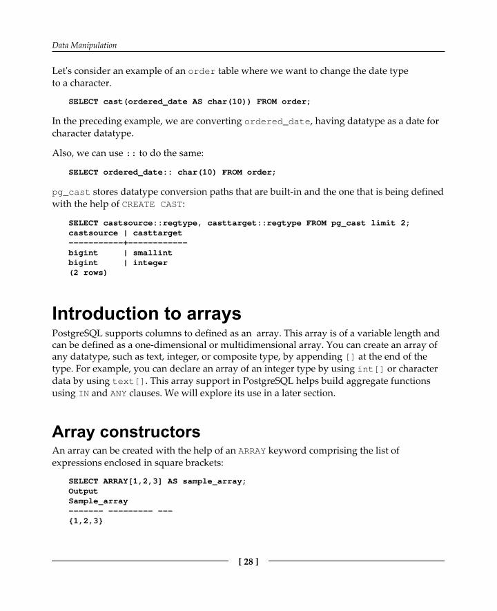
Let's consider an example of an order table where we want to change the date typeto a character.

SELECT cast(ordered_date AS char(10)) FROM order;

In the preceding example, we are converting ordered_date, having datatype as a date forcharacter datatype.

Also, we can use :: to do the same:

SELECT ordered_date:: char(10) FROM order;

pg_cast stores datatype conversion paths that are built-in and the one that is being definedwith the help of CREATE CAST:

SELECT castsource::regtype, casttarget::regtype FROM pg_cast limit 2;castsource | casttarget-----------+------------bigint | smallintbigint | integer(2 rows)

Introduction to arraysPostgreSQL supports columns to defined as an array. This array is of a variable length andcan be defined as a one-dimensional or multidimensional array. You can create an array ofany datatype, such as text, integer, or composite type, by appending [] at the end of thetype. For example, you can declare an array of an integer type by using int[] or characterdata by using text[]. This array support in PostgreSQL helps build aggregate functionsusing IN and ANY clauses. We will explore its use in a later section.

Array constructorsAn array can be created with the help of an ARRAY keyword comprising the list ofexpressions enclosed in square brackets:

SELECT ARRAY[1,2,3] AS sample_array;OutputSample_array------- --------- ---{1,2,3}

Data Manipulation

[ 29 ]

By default, the datatype of the preceding array will be an integer as it is the commondatatype for all members of sample_array. You can explicitly override the array datatypeto the other datatype by using the array constructor, for example:

SELECT ARRAY[1,2,3.2] :: integer[] AS sample_array;Sample_array------- --------- ---{1,2,3}

We can also define the array while defining the table and after that we can insert the data init.

Let's create a supplier table that has a product column:

CREATE TABLE supplier(name text, product text[])

In the preceding example, we created a table supplier with a text-type column for thename of the supplier, and a column product that represents the names of products havinga one-dimensional array.

Now, let's insert data in the preceding table and see how it looks:

INSERT INTO supplierVALUES('Supplier1','{ "table","chair","desk" }' )

We should use double quotes while inserting the members as the single quotes give anerror:

SELECT * FROM supplier;

Outputname | members----------+---------------------------Supplier1 | {table,chair,desk}(1 row)

We can insert the data using the array constructor as well:

INSERT INTO supplierVALUES(' Supplier2 ', ARRAY['pen','page '] )

Data Manipulation

[ 30 ]

While using the array constructor, the values can be inserted using single quotes:

SELECT * FROM supplier;

Output:name | members----------+---------------------------Supplier1 | {table,chair,desk}Supplier2 | {pen,page}

We can also get the values from another query and straightaway put them in an array.

Let's take an example where we want to put all the products in a single row. We have aproduct table that has product_id and product_name as columns. This can be done withthe help of the function array().

SELECT array(SELECT distinct product_name FROM supplier WHEREname='Supplier1') AS product_name;OutputProduct_name---- ---- ----- -----{table,chair, desk}

In the previous example, the inner query will fetch the distinct values of products whereasthe outer one will convert these into an array.

As discussed earlier, PostgreSQL supports multidimensional arrays as well. Let's consideran example to see how it works. Let's declare a table supplier that has aproduct_category column as a one-dimensional array and its product as a two-dimensional array:

CREATE TABLE supplier (name text,product_category text[],product text[][]);

Now, let's see how to insert the data in a two-dimensional array:

INSERT INTO supplier VALUES ('Supplier1', '{"Stationary","Books"}', '{{"Pen", "Pencil"}, {"PostgreSqlCookBook", "Oracle Performance"}}');

INSERT INTO supplier VALUES ('Supplier2', '{"LivingRoom Furniture"," Dinning Furniture"}', '{{"Sofa", "Table"}, {"Chair", "Cabinet"}}');

Data Manipulation

[ 31 ]

Since we have inserted the data in the two-dimensional array, let's query the suppliertable and check how the data looks:

SELECT * FROM supplier;

name | product_category | product-----------+--------------------------+-------------------------------Supplier1 | {Stationary,Books} | {{Pen, Pencil} {PostgreSqlCookBook,Oracle Performance}}Supplier2 | {LivingRoomFurniture,Dinning Furniture} | {{Sofa, Table}{Chair, Cabinet}}

In multidimensional arrays, extends of each dimension should match. A mismatch causesan error, for example: ERROR: multidimensional arrays must have arrayexpressions with matching dimensions.

A huge variety of array functions, are available in PostgreSQL. Let's discuss a couple ofthem.

String_to_array()PostgreSQL supports many array functions, one of which, is the string_to_arrayfunction. As the name states, this function helps convert the string into an array.

The following is the syntax for this function:

String_To_Array(String,delimeter)

String: This is the value that we need to convert to the arrayDelimeter: This will help you tell how the string needs to be converted to anarray

Let's take an example in which we have a string that we will convert into an array:

SELECT string_to_array ('This is a sample string to be converted into anarray',' ');OutputString_to_array--- ---- ----- ----- ----{This,is,a,sample,string,to,be,converted,into,an,array}

In the preceding example, we have taken delimeter as space so all the words that have aspace in between will be considered as individual members of the array.You can always goback and convert the array into a string using the other function array_to_string, whichworks in a similar manner.

Data Manipulation

[ 32 ]

Here is an example to convert an array into a string:

SELECT array_to_string (ARRAY[1, 2, 3], ',');Outputarray_to_string-----------------1,2,3

Array_dims( )We can check the dimensions of an array using the array_dims function. It will help usknow the number of values stored in an array. The following is the syntax:

Array_dims(column_name)

Let's take an example:

SELECT array_dims(product_category) FROM supplier;Outputarray_dims------------ [1:2] [1:2](2 rows)

Another example for a multidimensional array is as follows:

SELECT array_dims(product) FROM supplier;Outputarray_dims------------ [1:2] [1:2] [1:2] [1:2]

ARRAY_AGG()The ARRAY_AGG function is used to concatenate values including null into an array. Let'sconsider an example to see how it works:

SELECT name FROM supplier;name----|----Supplier1Supplier2(2 rows)

Data Manipulation

[ 33 ]

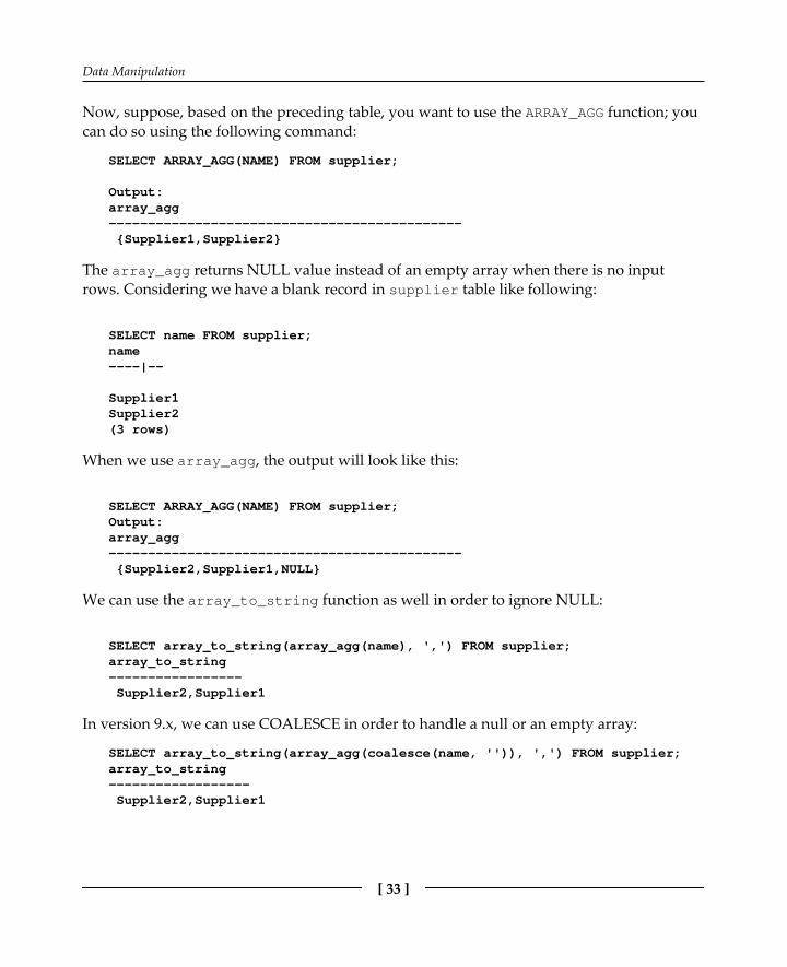
Now, suppose, based on the preceding table, you want to use the ARRAY_AGG function; youcan do so using the following command:

SELECT ARRAY_AGG(NAME) FROM supplier;

Output:array_agg--------------------------------------------- {Supplier1,Supplier2}

The array_agg returns NULL value instead of an empty array when there is no inputrows. Considering we have a blank record in supplier table like following:

SELECT name FROM supplier;name----|--

Supplier1Supplier2(3 rows)

When we use array_agg, the output will look like this:

SELECT ARRAY_AGG(NAME) FROM supplier;Output:array_agg--------------------------------------------- {Supplier2,Supplier1,NULL}

We can use the array_to_string function as well in order to ignore NULL:

SELECT array_to_string(array_agg(name), ',') FROM supplier;array_to_string----------------- Supplier2,Supplier1

In version 9.x, we can use COALESCE in order to handle a null or an empty array:

SELECT array_to_string(array_agg(coalesce(name, '')), ',') FROM supplier;array_to_string------------------ Supplier2,Supplier1

Data Manipulation

[ 34 ]

ARRAY_UPPER()The ARRAY_UPPER() function returns the upper bound of the array dimension. Thefollowing is the syntax for the same:

array_upper(anyarray, int)

Anyarray: This is the array column name or the array for which you want theupper bound

It will return the integer. The following is an example:

SELECT array_upper(product,1) FROM supplier WHERE name='Supplier1';

Array_upper---------2

Similarly, we can use the ARRAY_LOWER() function to check the lower bound of the array.

Array_length()This function returns the length of the requested array. The following is the syntax:

array_length(anyarray, int)

Anyarray: This is the array column name or the array for which you want theupper bound

It will return the integer. The following is an example:

SELECT array_length(product,1) FROM supplier WHERE name='Supplier1';

Array_length---------2

Array slicing and splicingPostgreSQL supports slicing an array, which can be done by providing the start and end ofthe array or the lower bound and upper bound of an array. It will be a subset of the arraythat you are trying to slice.

Data Manipulation

[ 35 ]

The following is the syntax:

lower-bound:upper-bound

Let's try to slice an array using the preceding syntax:

SELECT product_category[1:1] FROM supplier;

product_category-------+-----------------{Stationary} {LivingRoom Furniture}

We can also write the preceding query as follows:

SELECT product_category[1] FROM supplier;

If any of the subscripts are written in the lower:upper form, they are considered to beslices. If only one value is specified in the subscript, then, by default, the value of the lowerbound is 1, which means product_category[2] is considered as [1:2].

SELECT product[1:2][2] FROM supplier;product-------+----------------------------------- +------------------------------------{{Pen, Pencil}, {PostgreSqlCookBook, Oracle Performance}}

UNNESTing arrays to rowsPostgreSql supports a function that helps in expanding the array to rows, which means thatyou can expand the elements of the array to an individual record. This can be done with thehelp of unnest. Unnest can be used with multidimensional arrays as well.

The following is the syntax:

unnest(anyarray)

Let's take an example where we have the following content:

Product_category | product-----------------|-----------Furniture |chair,table,deskStationary |pencil,pen,book

SELECT Product_category, unnest(string_to_array(product, ',')) AS productFROM supplier;

Data Manipulation

[ 36 ]

Product_category | product-----------------|-----------Furniture |chairFurniture |tableFurniture |deskStationary |pencilStationary |penStationary |book

You can also directly put members of the array using the array syntax and then use unnest:

SELECT unnest(array[chair,table,desk]);unnest--------chairtabledesk(3 rows)

Also, PostgreSQL supports a multi-argument unnest as well. It behaves in the same way asa table using multiple unnest calls.

Let's take an example:

SELECT * FROM unnest(array[a,b],array[c,d,e]);unnest | unnest-------+--------a | cb | dNull | e

In the preceding example, we get a NULL value in the output because the array containsfewer values than some other array in the same table clause.

To use unnest with multiple arguments, you will need to make sure that the unnest is usedin the FROM clause rather than the SELECT clause, otherwise it will throw an error.

SELECT unnest(array[a,b],array[c,d,e]);ERROR: function unnest(integer[], integer[]) does not existLINE 1: SELECT unnest(array[a,b],array[c,d,e]);

Data Manipulation

[ 37 ]

Introduction to JSONPostgreSQL supports the JSON datatype, which is useful to store multilevel, dynamicallystructured object graphs. Although the data can be stored in text, the JSON datatype verifieswhether the value is in valid JSON format. There are two JSON datatypes: json and jsonb.Although they accept the same values as input, they have difference in their efficiency.Indexing is supported by jsonb.

The json datatype stores data as such due to which it has to reparse whileexecution. The jsonb datatype stores in binary format, which it convertsduring conversion, but it doesn't reparse during execution, so it is faster incomparison to json.

Inserting JSON data in PostgreSQLLet's create a table first in which we will have only two columns—id and data:

CREATE TABLE product_info (id serial, data jsonb);

Once the table is created, let's insert some data in it:

INSERT INTO product_info (data) VALUES('{"product_name":"chair","product_category":"Furniture","price":"200"}'),('{"product_name":"table","product_category":"Furniture","price":"500"}'),('{"product_name":"pen","product_category":"Stationary","price":"100"}'),('{"product_name":"pencil","product_category":"Stationary","price":"50"}');

Now, let's see how the data looks:

SELECT * FROM product_info;id | data----+-------------------------------------- 1 | {"product_name":"chair","product_category":"Furniture","price":"200"} 2 | {"product_name":"table","product_category":"Furniture","price":"500"} 3 | {"product_name":"pen","product_category":"Stationary","price":"100"} 4 | {"product_name":"pencil","product_category":"Stationary","price":"50"}

Data Manipulation

[ 38 ]

Querying JSONWhenever we develop a query to get a result, we will always use the comparison operatorto filter data.

Equality operationThis is only available for jsonb; we can get two JSON objects that are identical:

SELECT * FROM product_info WHERE data ='{"product_category":"Stationary"}';id | data----+---------------------------------------------------------------- (0 rows)

We got zero records because we don't have any record equal toproduct_category:Stationary.

ContainmentContainment means is a subset of. We can query if one JSON object contains another. Thisis, again, valid for jsonb only:

SELECT * FROM product_info WHERE data @>'{"product_category":"Stationary"}';

It will return all objects that contain the product_category key with the value stationary:

id | data---+---------------------------------------------------------------- 3 | {"product_name":"pen","product_category":"Stationary","price":"100"} 4 | {"product_name":"pencil","product_category":"Stationary","price":"50"}(2 rows)

The containment goes both ways:

SELECT * FROM product_info WHERE data <@'{"product_category":"Stationary"}';

Data Manipulation

[ 39 ]

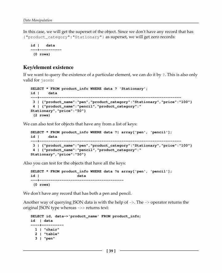
In this case, we will get the superset of the object. Since we don't have any record that has{"product_category":"Stationary"} as superset, we will get zero records:

id | data---+---------- (0 rows)

Key/element existenceIf we want to query the existence of a particular element, we can do it by ?. This is also onlyvalid for jsonb:

SELECT * FROM product_info WHERE data ? 'Stationary';id | data---+---------------------------------------------------------------- 3 | {"product_name":"pen","product_category":"Stationary","price":"100"} 4 | {"product_name":"pencil","product_category":"Stationary","price":"50"} (2 rows)

We can also test for objects that have any from a list of keys:

SELECT * FROM product_info WHERE data ?| array['pen', 'pencil'];id | data---+---------------------------------------------------------------- 3 | {"product_name":"pen","product_category":"Stationary","price":"100"} 4 | {"product_name":"pencil","product_category":"Stationary","price":"50"}

Also you can test for the objects that have all the keys:

SELECT * FROM product_info WHERE data ?& array['pen', 'pencil'];id | data---+-------------------------------------- (0 rows)

We don't have any record that has both a pen and pencil.

Another way of querying JSON data is with the help of ->. The -> operator returns theoriginal JSON type whereas ->> returns text:

SELECT id, data->'product_name' FROM product_info;id | data----+---------- 1 | "chair" 2 | "table" 3 | "pen"

Data Manipulation

[ 40 ]

4 | "pencil"

You can select rows based on values from the JSON field:

SELECT product_name FROM productWHERE data->>'product_category' = 'Stationary';product_name-------penpencil

Outputting JSONPostgreSQL also allows you to manipulate the existing tables and get the output in a JSONformat.

Let's create a normal table and insert data into it:

CREATE TABLE product_info (id serial, product_name text, product_categorytext, price int);INSERT INTO product_info (product_name ,product_category , price)VALUES ('Chair', 'Furniture', 200);

Now, since we have inserted the record in a normal way, we will change this to the JSONformat. We will use the row_to_json function:

row_to_json-----------------------------------------------{"f1":"Chair","f2":"Furniture","f3":200}(1 row)

The field names have default values generated automatically by PostgreSQL. Similarly, wecan output the array values as JSON with the help of the array_to_json function:

CREATE TABLE product_info(id serial, product_category text, producttext[]);INSERT INTO product_info (product_category , product) VALUES('Stationary', '{"Pen","Pencil"}');

Now, since the data has been inserted in the table, let's get this output as JSON:

SELECT row_to_json(row(product_category,array_to_json(product))) FROMproduct_info;

row_to_json----------------------------------------{"f1":"Stationary"," f2":['Pen','Pencil']}

Data Manipulation

[ 41 ]

(1 row)

Using XML in PostgreSQLLike the JSON dataype, PostgreSQL provides xml datatypes as well, which helps us instoring XML data.The xml datatype is perhaps one of the more controversial types you'llfind in a relational database. It comes with various functions to generate data, concatenate,and parse XML data, which we will discuss in further sections.

Inserting XML data in PostgreSQLLike the JSON datatype, the xml datatype also make sure whether we are inserting the validXML data or not. That is what makes the xml datatype different from a text datatype.

Let's create a table first and then we will insert data into it:

CREATE TABLE product_xml (id serial, info xml);

Now, since the product_xml table is created with a column having the xml datatype, let'sinsert some data in it:

INSERT INTO product_xml (info)VALUES ('<product category>"Furniture"><product_info><name> chair </name><price> 200</price></product_info><product_info><name> table </name><price> 500</price></product_info></product_category>');

We can always add a check constraint, making sure the price is always included with theproduct information using the xpath_exists function. This function basically evaluatesthe path of the XML string:

ALTER table product_xml add constraint check_priceCHECK(xpath_exists('/product_category/product_info/price',info));

Now, if you try to insert something like this:

INSERT INTO product_xml (info)VALUES ('<product category ="Furniture"></product_category>');

It will error-out, telling us that it violates the check_price constraint. Similarly, there is thexpath function as well, which we will discuss in the next section.

Data Manipulation

[ 42 ]

Querying XML dataTo query XML data, we can use the xpath() function. We will need to mention the path toget the required value. Let's consider querying the product_xml table, which we created inan earlier section:

SELECT xpath('/product_category/product_info/name/text()', product_info)FROM product_xml;Xpath----------Chairtable

It returns the value of product_ name.

Composite datatypePostgreSQL supports a special datatype called composite datatype. The composite typerepresents the structure of a record or a row, which means it will have a list of fields andtheir datatypes. PostgreSQL supports using composite types in multiple ways, similar tohow simple types can be used. A column of a table can be declared to be of a compositetype.

Creating composite types in PostgreSQLWe can create or declare a composite datatype using the following syntax:

CREATE TYPE composite_type_name AS (Column_name1 any_datatype,Column_name2 any_datatype..);

CREATE TYPE composite_type_name AS: With this, PostgreSQL will help uscreate a composite datatype. The composite_type_name is the name of thecomposite type you want to define.Column_name1 any_datatype: You can provide the column that you want todeclare accompanied by the datatype that you want to assign to the column.

The syntax of CREATE TYPE is similar to CREATE TABLE, except that you can only specifythe field names and types; constraints, such as NOT NULL, cannot be included as part ofthis.

Data Manipulation

[ 43 ]

Let's try to create a composite datatype of a product with further details:

CREATE TYPE product AS (Product_name text,price numeric,Product_category text);

In the preceding example, we created a type with a name product with Product_name,price, and Product_category columns .

Now, since we discussed how we can declare a composite datatype, let's see how to use thiscomposite type while creating a table:

CREATE TABLE supplier(Supplier_name text,Product_info product);

In the preceding example, we created the supplier table with a Supplier_name and aProduct_info column. The Product_info column is of product datatype, which willautomatically inherit its structure, including the column's product name, price, and productcategory.

There are two ways to insert data in composite columns. They are as follows:

You can insert it as a literal constant—the field values need to be enclosed withinparentheses and separated by commas. You can use double quotes around anyfield value, and must do so if it contains commas or parentheses. An example isshown, as follows:

INSERT INTO supplier VALUES ('Supplier1', '("Table", 1000,"Furniture")');

You can also use the ROW keyword while inserting the values in compositecolumns, but the ROW keyword is actually optional, except you have more thanone field in the expression. In this case, you will need to use single quotes for thetext field, as in the following example:

INSERT INTO supplier VALUES ('Supplier2', ROW('Chair', 500,'Furniture'));

Data Manipulation

[ 44 ]

We need to use the ROW keyword while inserting the field values in composite datatypecolumns, like we did in the previous example to insert data for the product datatype.

So far, we have seen how we can declare composite datatype columns and insert the data.Now, let's discuss how to access a field of a composite column. You can use a dot followedby the field name, the way you do while selecting a field from a table name. For example, toselect some subfields from our supplier table, we can use the following query:

SELECT (product_info).product_nameFROM supplierWHERE (product_info).price > 500;

You can also use the table name, in which you have multiple tables, as shown in thefollowing query:

SELECT (supplier.product_info).product_nameFROM supplierWHERE (supplier.product_info).price > 500;

Product_name-------------Table

Altering composite types in PostgreSQLTo alter the definition of an existing composite type, we can use the ALTER TYPE keyword.There can be many things that we want to alter in a composite type, such as adding orremoving a column. In this section, we will discuss similar scenarios.

To add a column in an existing composite type, we can use the following syntax:

ALTER TYPE type_name ADD ATTRIBUTE attribute_namedata_type[ COLLATEcollation ] [ CASCADE | RESTRICT ]

ALTER TYPE: This changes the definition of an existing type.ADD ATTRIBUTE: This adds a new attribute to a composite type.CASCADE: This automatically applies the change to the table that we are using, thetype which is being altered, and its successors.RESTRICT: This refuses the operation if the type is used by a typed table. This isthe default.

Data Manipulation

[ 45 ]

Now, let's add a column in product type:

ALTER TYPE product ADD ATTRIBUTE unit_of_measureint CASCADE;

Similarly, to remove a column from ALTER TYPE type_name DROP ATTRIBUTE [ IFEXISTS ] attribute_name [ CASCADE | RESTRICT ]:

DROP ATTRIBUTE [ IF EXISTS ]: This form drops an attribute from acomposite type. If IF EXISTS is specified and the attribute does not exist, noerror is thrown.

ALTER TYPE product DROP ATTRIBUTE unit_of_measureint CASCADE;

The same syntax will be used to alter the value of an attribute:

ALTER TYPE type_name ALTER ATTRIBUTE attribute_name [ SET DATA ] TYPE data_type [ COLLATE collation ] [ CASCADE | RESTRICT ]

SET DATA TYPE: This form changes the datatype of the attribute.

Dropping composite types in PostgreSQLYou can drop a composite type with the help of DROP TYPE. Simply using DROP TYPE willnot drop any dependent tables, so you will have to use CASCADE like below:

DROP TYPE product CASCADE;

SummaryIn this chapter, we looked at ways in which we can use the functionality of PostgreSQLusing arrays, slicing arrays, and unnesting arrays of rows. An array provides greatfunctionality when it comes to using data in multiple ways, or when we have a large chunkof data available with us. We also looked at the JSON datatype, which is useful to storemultilevel, dynamically structured object graphs. Additionally, we discussed how tomanage XML data and use its functions, which is supported by PostgreSQL. In the lastsection, we looked at ways to deal with composite types and altering types. Compositetypes are pretty important as once created they can be referred to by multiple tables, whichhelps in avoiding the same set of attributes again and again. Also, if we need to altersomething in the set of those attributes, we will need to do it once and it will beautomatically reflected in the dependent tables.

3Triggers

In the previous chapter, we talked about a few data manipulation concepts of PostgreSQL;different complex data types, such as array, JSON, and XML; and how to handle them. Inthis chapter, we will discuss the basics, which will help you understand how triggers workin PostgreSQL and how to manage the PostgreSQL trigger, including modifying, disabling,and removing the trigger. Additionally, we will discuss trigger functions as well.

Introduction to triggersA trigger is a specification that the database should run automatically whenever a certaintype of operation is performed. It can be defined to run or fire either before or after anyINSERT, UPDATE, or DELETE operation is performed on a particular object. This operationcan be associated with a table, a view, a schema, or the database, and it is one of thefollowing:

A Data Manipulation Language (DML) statement—DELETE, INSERT, or UPDATEA Data Definition Language (DDL) statement—CREATE, ALTER, or DROPA database operation—SERVERERROR, LOGON, LOGOFF, STARTUP, or SHUTDOWN

Like a stored procedure, a trigger can be invoked repeatedly. A procedure is explicitly runby a user or an application but triggers are implicitly fired when a triggering event occurs,no matter which user is connected or which application is used. It can be enabled anddisabled but you cannot explicitly invoke it. While a trigger is enabled, the databaseautomatically invokes it—that is, the trigger fires—whenever its triggering event occurs.While a trigger is disabled, it does not get fired.

Triggers

[ 47 ]

There are two type of triggers based on the level they are triggered at:

Row-level trigger: An event is triggered for each row updated, inserted, ordeletedStatement-level trigger: When a SQL statement emits an event, any triggers thatare registered to listen for that event will be fired

Adding triggers to PostgreSQLYou can create a trigger with the CREATE TRIGGER statement. You are required to specifythe triggering event in terms of triggering statements and the item on which they get fired.By default, a trigger is created in the enabled state.

The basic CREATE TRIGGER syntax is as follows:

CREATE [OR REPLACE ] TRIGGER trigger_name{BEFORE | AFTER | INSTEAD OF} {event [OR ...]}ON table_name[FOR [EACH] {ROW | STATEMENT}]EXECUTE PROCEDURE trigger_function;

Let's discuss the parameters of the preceding code syntax:

CREATE [OR REPLACE ] TRIGGER trigger_name: This creates a trigger withthe given name or overwrites an existing trigger with the same name.BEFORE | AFTER | INSTEAD OF: This indicates the time when the triggershould get fired, for example, before or after updating a table. INSTEAD OF isused to create a trigger on a view. BEFORE and AFTER cannot be used to create atrigger on a view.{INSERT [OR] | UPDATE [OR] | DELETE}: This determines what operation atrigger should get fired at. The OR keyword can be utilized to use more than onetriggering event. The trigger gets fired at all the specified triggering events.[ON table_name]: This identifies the name of the table or view with which thetrigger is associated.[FOR EACH ROW]: This is used to determine whether a trigger must fire wheneach row gets affected (a row-level trigger) or just once when the entire SQLstatement is executed (a statement-level trigger).WHEN (condition): This is valid only for row-level triggers. It is fired only forrows that satisfy the condition specified.

Let's create a trigger that helps in maintaining the history of employee salaries.

Triggers

[ 48 ]

We can create a trigger to update the emp_salary_history table when an employee'ssalary is updated in the employee table.

First, we will create the employee table and the emp_salary_history table:

CREATE TABLE employee(emp_id int4,employee_name varchar(25),department_id int4,salary numeric(7,2));

CREATE TABLE emp_salary_historyemp_id int,,employee_name varchar(25),salary numeric(7,2)Changed_on timestamp(6));

First, we will define a new function called insert_into_salary_history:

CREATE OR REPLACE FUNCTION insert_into_salary_history()RETURNS trigger AS$BODY$BEGININSERT INTO emp_salary_history VALUES(:old.emp_id, :old.employee_name, :old.salary, Now());END;$BODY$

Let's create emp_history_trigger and execute it. This trigger will help you in insertingvalues in the employee history table before updating the employee table.

CREATE or REPLACE TRIGGER emp_history_triggerBEFORE UPDATE OF salaryON employeeFOR EACH ROWEXECUTE PROCEDURE insert_into_salary_history();

Lets insert the data in the employee table:

INSERT INTO employee (emp_id,employee_name,department_id,salary)VALUES (1, 'John',100,25000);INSERT INTO employee (emp_id,employee_name,department_id,salary)VALUES (2, 'Doe',110,30000);

Triggers

[ 49 ]

And this is what the data will look like in the table:

SELECT * FROM employee;

emp_id employee_name department_id Salary

1 John 100 25000

2 Doe 110 30000

Now, let's update the salary of an employee:

UPDATE EMPLOYEE SET salary = 26000 WHERE emp_id = 100

Let's see how the data looks after the update:

SELECT * FROM employee;

emp_id employee_name department_id Salary

1 John 100 26000

2 Doe 110 30000

Once the preceding update query is executed, the trigger gets fired and it inserts data in theemp_salary_history table.

To view the records run the following query:

SELECT * FROM emp_salary_history;

emp_id employee_name Salary Changed_on

1 John 25000 2015-05-12 15:21:00

If you ROLLBACK the transaction before committing to the database, the data inserted intothe table is also rolled back.

Let's take another example. We discussed the different types of trigger earlier—row-leveltriggers and statement-level triggers. Through this example, we will see how it works.

This is the hierarchy followed when a trigger is fired. The BEFORE statement's trigger firesfirst. Next, the BEFORE row-level trigger fires, once for each row affected. Then the AFTERrow-level trigger fires, once for each affected row. These events will alternate betweenthe BEFORE and AFTER row-level triggers. Finally, the AFTER statement-level trigger fires.

Triggers

[ 50 ]

Let's create a table, emp_msg, which we can use to store messages when triggers are fired:

CREATE TABLE emp_msg(Message varchar(40), CurrentDate timestamp(15));

Let's create a BEFORE and AFTER statement and row-level triggers for the employee table:

BEFORE UPDATE, statement level: This trigger will insert a record into theemp_msg table before a SQL update statement is executed at the statement level

CREATE OR REPLACE FUNCTION Before_Update_Stat_employee_fnc() RETURNS trigger AS $BODY$ BEGIN INSERT INTO emp_msg Values('Before update, statement level',now()); END; $BODY$

CREATE or REPLACE TRIGGER Before_Update_Stat_employee BEFORE UPDATE ON employee FOR EACH ROW EXECUTE PROCEDURE Before_Update_Stat_employee_fnc();

BEFORE UPDATE, row level: This trigger will insert a record into theemp_msg table before each row is updated

CREATE OR REPLACE FUNCTION Before_Update_Row_employee_fnc() RETURNS trigger AS $BODY$ BEGIN INSERT INTO emp_msg Values('Before update, row level',now()); END; $BODY$

CREATE or REPLACE TRIGGER Before_Update_Row_employee() BEFORE UPDATE ON employee FOR EACH ROW EXECUTE PROCEDURE Before_Update_Row_employee_fnc();

AFTER UPDATE, statement level: This trigger will insert a record into theemp_msg table after a SQL update statement is executed at the statement level

CREATE OR REPLACE FUNCTION After_Update_Stat_employee_fnc() RETURNS trigger AS $BODY$

Triggers

[ 51 ]

BEGIN INSERT INTO emp_msg Values('After update, row level',now()); END; $BODY$

CREATE or REPLACE TRIGGER After_Update_Stat_employee() BEFORE UPDATE ON employee FOR EACH ROW EXECUTE PROCEDURE After_Update_Stat_employee_fnc();

AFTER UPDATE, row level: This trigger will insert a record into the emp_msg tableafter each row is updated

CREATE OR REPLACE FUNCTION After_Update_Row_employee_fnc() RETURNS trigger AS $BODY$ BEGIN INSERT INTO emp_msg Values('After update, row level',now()); END; $BODY$

CREATE or REPLACE TRIGGER After_Update_Row_employee() BEFORE UPDATE ON employee FOR EACH ROW EXECUTE PROCEDURE After_Update_Row_employee_fnc();

Now, let's execute an update statement on the table product:

UPDATE employee SET salary = 20000 WHERE emp_id IN (100,101);

Let's check the data in the emp_msg table to see the order in which the trigger is fired:

SELECT * FROM emp_msg order by current_date;Output:Mesage Current_Date------------------------------------------------------------Before update, statement level 12-May-2015Before update, row level 12-May-2015After update, Row level 12-May-2015Before update, row level 12-May-2015After update, Row level 12-May-2015After update, statement level 12-May-2015

Triggers

[ 52 ]

The preceding result shows that the before update and after update row-level events haveoccurred twice as two records were updated. But the before update and after updatestatement-level events are fired only once for each SQL statement.

The preceding rules apply similarly to the INSERT and DELETE statements.

Modifying triggers in PostgreSQLIn order to modify the existing trigger, you can use the ALTER TRIGGER statement. TheRENAME clause changes the name of the given trigger without otherwise changing thetrigger definition. The syntax of the ALTER TRIGGER statement is as follows:

ALTER TRIGGER trigger_name ON table_nameRENAME TO new_name;

ALTER TRIGGER: This statement helps you in modifying the existing triggertrigger_name: This is the name of an existing trigger to alterTable_name: This is the name of the table on which this trigger gets firedNew_name: This is the new name for the trigger

Let's consider an example where you want to change the name ofthe emp_history_trigger trigger , which is associated with the employee table, toemployee_salary_history_trigger. You can use the ALTER TRIGGER as follows:

ALTER TRIGGER emp_history_trigger ON employeeRENAME TO employee_salary_history_trigger;

You can also disable an existing trigger using the ALTER TRIGGER command. The followingis the syntax to disable the trigger with the ALTER statement:

ALTER TABLE table_nameDISABLE TRIGGER trigger_name | ALL

ALTER TABLE table_name: This clause will alter the table on which the triggeris based.DISABLE TRIGGER trigger_name | ALL: This clause will disable the giventrigger. If you want to disable all the triggers, then you don't need to mention thetrigger name, and you can use the ALL keyword.

Triggers

[ 53 ]

A disabled trigger will still exist in the database. It will not get fired whenits triggering event occurs.

If you want to disable the employee_salary_history_trigger associated with theemployee table, you can use the following statement:

ALTER TABLE employeeDISABLE TRIGGER employee_salary_history_trigger;

Removing a trigger functionTo remove an existing trigger definition, you can use the DROP TRIGGER statement, asfollows:

DROP TRIGGER [ IF EXISTS ] name ON table_name [ CASCADE | RESTRICT ]

IF EXISTS: This will not throw an error if the trigger does not exist.name: This is the name of the trigger that has to be to removed.table_name: This is the name, optionally schema-qualified, of the table forwhich the trigger is defined.CASCADE: This automatically drops the objects that depend on the trigger.RESTRICT: This refuses to drop the trigger if any objects depend on it. This is thedefault. You can specify the trigger name that you want to remove after the DROPTRIGGER clause and the table with which the trigger is associated.

For example, to remove the employee_salary_history_trigger trigger, you can use thefollowing statement:

DROP TRIGGER employee_salary_history_trigger ON employee CASCADE;

The preceding code line will drop all the objects that are dependent onemployee_salary_history_trigger.

DROP TRIGGER employee_salary_history_trigger ON employee RESTRICT;

The preceding code line is by default and will not drop the trigger if any objects depend onit.

Triggers

[ 54 ]

Creating a trigger functionPL/pgSQL allows us to make a trigger function. This trigger function is similar to anordinary function but it does not have any parameter and has a return type trigger. Atrigger fires when a condition is met and executes a special type of stored procedure calleda trigger function.

PostgreSQL will call a trigger function when changes are being made to a particular table.The function must either return NULL or a row that matches the structure of the table forwhich the trigger function has been called.

As mentioned earlier, the trigger function is created as an ordinary function. The followingis the syntax to create this:

CREATE FUNCTION trigger_function() RETURN trigger AS

The trigger function receives data about their calling environment through a specialstructure called TriggerData, which contains a set of local variables. For example, OLD andNEW represent the states of a row in the table before or after the triggering event.PostgreSQL provides other local variables with TG_ as the prefix, such as TG_WHEN,TG_TABLE_NAME, and so on. Let's discuss these procedure variables in more detail.

The PostgreSQL trigger procedure variables are as follows:

NEW: This is a record containing the new database rowOLD: This is a record containing the old database rowTG_NAME: This is a variable containing the name of the trigger that fired andcaused the trigger procedure to runTG_WHEN: This is a text variable containing the text before or after, depending onthe type of the triggerTG_LEVEL: This is a text variable containing the row or statement, depending onthe trigger definitionTG_OP: This is a text variable containing INSERT, DELETE, or UPDATE, dependingon the event that occurred resulting in this trigger being firedTG_RELID: This is an object identifier representing the table the trigger isactivated onTG_RELNAME: This is the name of the table that the trigger has been fired onTG_NARGS: This is an integer variable containing the number of argumentsspecified in the trigger definitionTG_ARGV: This is an array of strings containing the procedure parameters startingat zero; the invalid indexes return NULL values

Triggers

[ 55 ]

Testing the trigger functionLet's create a trigger function to capture the history transferred from multiple departments.

We have an employee table with the following structure:

CREATE TABLE employee( Emp_id int4, emp_name varchar(40), dept_id int4, salary numeric(7,2));

We also have an employee_dept_history table with the following structure:

CREATE TABLE employee_dept_history( Emp_id int4, emp_name varchar(40), dept_id int4, date_changed_on timestamp(6));

Now, let's create the trigger function:

CREATE OR REPLACE FUNCTION emp_dept_changes()RETURNS trigger AS$BODY$BEGINIF NEW.dept_id <> OLD.dept_id THENINSERT INTO employee_dept_history (emp_id,emp_name,dept_id,date_changed_on)VALUES(OLD.id,OLD.emp_name,OLD.dept_id,now());END IF;RETURN NEW;END;$BODY$ LANGUAGE 'plpgsql';

The function checks whether the department ID of the employee changes. It will insert theold department ID into the employee_dept_history table, including the employee ID,department ID, and the date of change.

Additionally, within this trigger function, two very special records are made available: OLDand NEW. These records contain (for row triggers) the data from the row being affected bythe UPDATE that fired the trigger. The OLD contains data from before the UPDATE, and NEW contains data from after the update (or the proposed UPDATE for a BEFORE trigger).

Triggers

[ 56 ]

Now, we will create the trigger that will use the trigger function. Before the department IDcolumn is updated, the trigger function is automatically invoked to log the change.

CREATE TRIGGER emp_dept__changes_trg BEFORE UPDATE ON employee FOR EACH ROW EXECUTE PROCEDURE emp_dept_changes ();

We can insert some sample data to test. We will insert two records into the employee table,as shown in the following code snippet:

INSERT INTO employee (emp_id, emp_name, dept_id, salary)VALUES ('1', 'John','100','25000');

INSERT INTO employee (emp_id, emp_name, dept_id, salary)VALUES ('2', 'Doe','101','30000');

The employee table has two records now.

Let's update the department ID of emp_id = 1:

UPDATE employeeSET dept_id= '102'WHERE emp_id = 1;

The trigger function is called whenever an UPDATE takes place on the employee table.When we run the update query, before updating the record,the emp_dept__changes_trg trigger will get fired, which in turn will call the triggerfunction, emp_dept_changes. The trigger function will check if the old department ID,which is 100, matches the new department ID, which is 102. As they are not equal, it willinsert the data in the employee_dept_history table.

Viewing existing triggersIn order to view all the triggers that exist in the database, you can query the PG_TRIGGERtable. This stores information about the header and body of the trigger.

SELECT * FROM pg_triggerWHERE tgname = 'employee_salary_history_trigger';

The preceding query provides the header and body of theemployee_salary_history_trigger trigger.

Triggers

[ 57 ]

SummaryIn this chapter, we looked at ways in which we can extend the functionality of PostgreSQLqueries through triggers. You learned that PostgreSQL triggers can use trigger functions,which enhance the functionality of triggers. As discussed in this chapter, triggers can beused as an alternative method to implement referential integrity constraints. By usingtriggers, business rules and transactions are easy to store in the database and can be usedconsistently even if there are future updates to the database. When a change happens in adatabase, a trigger can adjust the change to the entire database using the INSERT, UPDATE,or DELETE statements. In the next chapter, we will talk about some important aspects ofdatabase design, what makes a good database, and database design practices.

4Understanding Database

Design ConceptsWhen it comes to designing a database, it is very important that we understand databasedesign concepts first. Having less understanding or having some doubts, can lead to a baddatabase design, which can give rise to a number of problems for users, some of which areas follows:

Inability to fulfill report requirementLoss of data integrity over timeRedundancyBad performancePrimary key on multiple fields

Basic design rulesThere are some basic design rules which help us to build a good database. Let us discuss onthose:

The ability to solve the problemThe main reason for designing a database is to solve a problem. So, it's very important tounderstand the problem and build the database so that it can fulfill the businessrequirements. No matter how well a database is designed, it is worthless if it doesn't solvethe reporting requirements.

Understanding Database Design Concepts

[ 59 ]

The ability to hold the required dataThe main reason for having a database is to store data. While thinking about this concept,you should first consider what is required in order to fulfill the needed queries, the musthave fields and after that, you can go ahead and extend the design so that it can fulfill anyfuture requirements.

The ability to support relationshipsRelationships are equally as important as defining the entities. A database should supportrelationships among the entities. If you don't focus on the relationships, your databasedesign will end up excessively complex and might suffer from data integrity issues.

The ability to impose data integrityData integrity plays a very vital role in a database. The entire purpose of the database is tostore correct and high-quality data so that it can provide useful information when needed.Many real-time databases may have deficiencies because of handwritten forms that havemissing information. This is just one example of data integrity that may cause furtherdeterioration in the quality of the data.

The ability to impose data efficiencyIn a largely built database, there are cases where performance may not be up to the desiredexpectations. And, achieving more practical goals may spoil the purity of the design. Thesteps for the optimized design should be considered with the utmost priority before youeven consider any optimization. A properly indexed database may drastically improve theperformance of the database. Another simple method can be to rewrite queries, which canprovide dramatic performance improvements without hampering the core design. Thingsthat you can avoid to maintain the database is changing a varchar to the char type orexperimenting with indexes on different attributes. This is just a waste of time andresources that will result in a poor performance and inconsistent database schema, which isdifficult to maintain. The first and foremost step is to check and provide the solution in theapplication design if there are any bottlenecks. Redesigning the database should be the lastresort when it comes to an optimized system. With this consideration, a quote stated fromDonald Knuth (Professor Emeritus of The Art of Computer Programming at StanfordUniversity), “Premature optimization is the root of all evil”, should make more sense now.

Understanding Database Design Concepts

[ 60 ]

The ability to accommodate future changesIn the software industry, people are generally surprised at just how long software remainsin use, even well beyond the design's lifetime. And when it comes to databases, thisbecomes even more noticeable. The reason for this is that, migrating the data from an oldlegacy system to the new one is often a significant problem in its own right. There is alwaysa constant pressure to enhance the existing database design rather than start from scratchand then migrate the data at a later stage. It's often noticeable that any change that youmake to your database to improve the efficiency makes your design harder to evolve.

NormalizationNo database design is complete without discussing database anomalies, normal forms, anddatabase normalization. As we have gone through the various design stages, we can nowsee how the final design will be formed based on these rules. The origin of databasenormalization was revealed by E.F. Codd in 1969, published in Communications of the ACM,Vol. 13, No. 6, June 1970.

In this work, normal forms were defined and each normal form was built on a previous ruleand applies more stringent requirements to the design. In a religious normalization theory,there are five normal forms, for example, the Boyce-Codd normal form. But in reality, youwill be amazed to know that only the first three forms are commonly used, and we willdiscuss them in the detail in this chapter.

A normalized database is easy to maintain and manage. All of this can be achieved usingthe first three normal forms. Databases that are designed without keeping in mindnormalization will always have performance issues and are more inclined to store invaliddata.

Anomalies in DBMSBroadly, we have three types of anomalies that will occur when the database is notnormalized. These are the insertion, update, and deletion anomalies. Let's consider each oneof them with an example.

Understanding Database Design Concepts

[ 61 ]

For example, suppose a company stores employee details in a table named employee thathas four attributes: emp_id to store the employee's id, emp_name to store the employee'sname, emp_address to store the employee's address, and emp_dept to store thedepartment details (where the employee works). At the initial stage, the table will look likethis:

emp_id emp_name emp_address emp_dept

101 Roger Texas D001

101 Roger Texas D002

123 Martin Ohio D890

166 George New York D900

166 George New York D004

As you can see, the preceding table is not normalized. We will start to see the followingproblems when a table is not normalized:

Update anomaly: In the preceding table, we have two rows for employee Georgeas he belongs to two departments of the company. If we want to update theaddress of George, then we have to update it in two rows or the data will becomeinconsistent. If, somehow, the correct address gets updated in one departmentbut not in the other, then, as per the database, George will have two differentaddresses, which is not correct and will lead to inconsistent data.Insert anomaly: Suppose a new employee joins the company, and is undertraining and currently not assigned to any department, then we will not be ableto insert the data into the table if the emp_dept field doesn't allow nulls.Delete anomaly: Suppose, the company closes the department D890, thendeleting the rows that have emp_dept as D890 will also delete all the informationfor employee Martin, as he is assigned only to this department.

To overcome these anomalies, we will need to normalize the data. In the next section, wewill discuss normalization.

Understanding Database Design Concepts

[ 62 ]

First normal formIn linewith the rule of first normal form (1NF), an attribute (column) of a table cannot holdmultiple values. It should hold only atomic values and it cannot be further subdivided intorepeating groups. For example, in our database design, we divided the vendor name intoa title, first name, and last name. There may arise a situation where we will have to usethem separately. So, storing them as individual attributes will allow us to achieve this.

Having no repeating groups suggests that the data should be consistent and the groups forany employee should not be repeated. A simple example to explain this will be using asimple worksheet to store vendors and their orders. Once a vendor has more than oneorder, we have repeating information for that vendor, and our worksheet will no longerhave the same number of rows in all columns.

If we store both the first and last name in the fname column of our Vendor table, then thiswill go against the 1NF because the column fname will actually be holding both the names.We will need to store the names separately so that consistency can be maintained.

Second normal formA table is said to be in the second normal form (2NF) if:

It is in 1NFNo nonprime attribute is dependent on the proper subset of any candidate key ofthe table

In other words, it means that no information in a row depends on only a part of the primarykey. For example, in our ORDERINFO table, we stored the date that the order was placed inthis table, as shown in the following table:

Column name Datatype

ORDER_ID INTEGER

ITEM_ID INTEGER

NO_OF_QUANTITY INTEGER

DATE_ORDER_PLACED DATE

Understanding Database Design Concepts

[ 63 ]

In the preceding table, (ORDERINFO), we can see that the breaking 2NF will recall that ourprimary key for ORDERINFO is a candidate key of ORDER_ID and ITEM_ID. The date onwhich the order was placed depends on only the ORDER_ID column, and not on the itemordered. Therefore, this will have violated 2NF.

In some scenarios, you may encounter that you are storing data that looks as if it might goagainst the 2NF but, in reality, it does not. For instance, if we change our prices frequently,customers will rightly expect to pay the price shown on the day they ordered and not on theday it was shipped.

In order to accomplish this, we will need to store the selling price in the ORDERINFO table torecord the price on the date on which the order was placed. This will not violate 2NF,because the price stored in the ORDERINFO table will depend on both the item and the actualorder.

Third normal formA table is said to be in third normal form (3NF) if both the following conditions are true:

The table must be in 2NFTransitive functional dependency of nonprime attribute on any super key shouldbe removed

An attribute that is not part of any candidate key is known as a nonprime attribute. Thisform is very closely tied to the 2NF but is more general. It says that no information in anattribute that is not the primary key can depend on anything except the primary key.

Suppose, in the Vendor table, we stored a vendor's age and DOB as shown in the followingtable. This will violate 3NF because the vendor's age depends on the DOB, a non-keycolumn, as well as the actual customer, which is given by VENDOR_ID (primary key).

Column name Datatype

VENDOR_ID INTEGER

TITLE VARCHAR (4)

FIRST NAME VARCHAR (100)

LAST NAME VARCHAR (100)

ADDRESS VARCHAR (100)

POSTAL CODE VARCHAR (100)

Understanding Database Design Concepts

[ 64 ]

COUNTY VARCHAR (100)

COUNTRY VARCHAR (100)

DOB DATE

Although the preferred solution is to make your database reach to the 3NF, there aresituations when it's necessary to break the rules. This process is called denormalizing thedatabase. You should always consider designing the database in a fully normalized way.However, you can denormalize it when you have a major problem with performance.

Common patternsThere are many situations that will occur repeatedly when you design or build a database.We normally call them common patterns. It is very important that you understand thesepatterns as they are solved in the same way, or the strategy to solve them will be similar,and that will save your time. Here, we will discuss some common problems and patternsand how we can solve or implement them.

Many-to-many relationshipsBefore we discuss how to implement a many-to-many relationship, let's discuss whatexactly this many-to-many relationship is.

If a row in a table is associated with one or more rows in other table and a row in other tableis associated with one or more rows in first table, then it's called many-to-manyrelationship. An example of a many-to-many relationship is a table of orders and products.Now, one order might have one or more products and a product can be ordered by one ormore orders.

It is never recommended you implement a many-to-many relationship in a database, so youwill need to insert a table that will have a one-to-many relationship with both the maintables. We call it the Link table. Now, this particular table will have a primary key fromboth the tables. So, the primary key of the first table or the primary key of the second tablemay occur multiple times but the combination of both primary keys, which we can use asthe surrogate key, will exist only once.

Understanding Database Design Concepts

[ 65 ]

Let's consider the preceding example using Orders and Products. In order to implementa many-to-many relationship between two, take the third table, as order details.

Now Order id is the primary key of the Orders table and Product id is the primary keyof the Products table. Both are foreign keys in the Order details table. But, together,they form a surrogate key in the Order details table and will form a primary key there,which means that the combination of Order id and Product id will be unique.

HierarchyAnother pattern is a hierarchy. Now, a hierarchy is basically a parent-child relationship.Suppose we have a product inventory that is located in a state and country; you canimplement the following model, which is not ideal:

Understanding Database Design Concepts

[ 66 ]

The problem with this model is that, while inserting the Country id, there is no constraintthat will check whether the state comes under what Country, which doesn't complete thehierarchy as such.

In order to make sure that a parent-child relationship is followed, we can implement thefollowing model, which makes sure that the hierarchy is maintained, and also a directrelationship between State and Country.

Recursive relationshipsThis is another pattern commonly encountered while building a database. So far, we havetalked about the relationships between two entities or tables. But, there can also be ascenario where an entity has a relationship with itself, which we call a recursiverelationship.

Let's consider a basic example of Employee and Supervisor. In every department, anemployee is supervised by a supervisor and of course, all the employees are notsupervisors. So, in order to visualize this example, refer to the following diagram:

Understanding Database Design Concepts

[ 67 ]

Although, for visualization, the preceding diagram is okay, this is not the correct way toachieve it in a database. The problem with this model is that each manager is also anemployee. If we build the Supervisor table, we will have duplicate information in bothtables, which will lead to redundancy.

In order to implement a recursive relationship in a database, it is better to add anothercolumn as supervisor_id to record which employee is supervised by whom and relate itto the same table.

Now, the Supervisor field will have an employee ID for the supervisor. In order to queryemployees and their supervisors, we will join the Employee table to itself using aliases.

SELECT e.emp_name AS "Employee name", m.emp_name AS "Manager name"FROM Employee e LEFT OUTER JOIN Employee MON E.supervisor_id = M.emp_iD

We have an outer join here in order to make sure that the employees also comes in theresult that is not supervised by anyone.

SummaryIn this chapter, we talked about what problems you will face if your database is notdesigned properly and how to overcome them. It gives you a good idea of what we shouldkeep in mind while designing a database. Additionally, we also discussed databaseanomalies, normal forms, and database normalization. In the next chapter, we will talkabout transactions and locking. We will cover how to start and manage a transaction usingdifferent kinds of isolation level. We will explain each kind of transaction level withexamples. We will also cover the locking mechanism available in PostgreSQL and how wecan best use it to benefit from locking.

5Transactions and Locking

So far in this book, we have discussed basic and advanced concepts of PostgreSQL and afew database designing concepts. In this chapter, we will discuss multiuser aspects ofPostgreSQL. In the real world, an application being accessed by multiple users at the sametime is very generic and it becomes important that we understand these concepts. We willlook at two important concepts of database support for multiple users: transactions andlocking.

Transaction means a combination of different changes made to the database in a single unit.And when we talk about multiuser environment, which means that multiple users aretrying to access the database at the same time, it's very important that multiple transactionsare not impacting each other. So, we will discuss the challenges that we face in multiuserenvironments and different levels of isolation, which is required to control the concurrency.Additionally, we will discuss the different techniques of locking.

Defining transactionsIn the previous chapters, we mentioned that we should try and write all the databasechanges with a single declarative statement. However, when it comes to reality, there comesa time when you cannot write everything to a database using one single SQL statement.This doesn't mean it will be just one single SQL statement; there might be multiplestatements that will update the database correctly. If, by chance, any problem is encountered in the statement or a group of statements, then none of the database changesshould be written. In other words, you will require the SQL statements to work as anindividual unit and execute tasks sequentially in a way that allows the changes to bereversed and hides uncommitted changes from other processes. In this case, either all of thestatements should be executing successfully or none of them should be executing.

Transactions and Locking

[ 69 ]

A real-world example can be taken from the banking domain, where all transactions arerecorded in debit and credit. So, we can consider the case of two accounts in the bankresiding in different tables in the database so that, when one account is debited, the othershould be credited. If, in any case, you debit one account and fail to credit the secondaccount, you must return the money to the first account. In other words, you act as ifnothing happened in the first place. No bank will remain in business if the moneydisappears when transferring between accounts.

For example, let's consider that we want to record a payment of $1,000 from John's accountto Smith's account. Using SQL statements, the situation will look like this:

UPDATE accounts SET balance = balance - 1000WHERE name = 'John';

UPDATE branches SET balance = balance - 1000WHERE name = (SELECT branch_name FROM accounts WHERE name = 'John');

UPDATE accounts SET balance = balance + 1000WHERE name = 'Smith';

UPDATE branches SET balance = balance + 1000WHERE name = (SELECT branch_name FROM accounts WHERE name = 'Smith');

With the preceding statements, as you can see, there are several steps involved when doingsimple debit and credit operations. The bank official will have to make sure that either allthese updates happen or none of them happen. So, we will need to guarantee that ifsomething goes wrong midway then none of the steps executed so far should take effect.We can achieve this guarantee if we group the update statements together. A transaction issaid to be atomic from the point of view of other transactions; it either happens completelyor not at all.

ACID rulesAtomicity, Consistency, Isolation, and Durability (ACID) is a frequently used acronym todescribe the four properties a transaction must have:

Atomicity: A transaction, no matter if it contains multiple actions on thedatabase, should happen as a one-individual unit. It should happen only once,with no repetition of the actions. In our banking example, the money movementmust be atomic. The debiting of one account and crediting of another must takeplace as one single action, no matter how many SQL statements are a part of thatunit.

Transactions and Locking

[ 70 ]

Consistency: The point of consistency is that there is no point where thetransaction is partially committed. In our banking example, all the accountsmaintained by the bank should accurately reflect the correct debit and creditbalances; otherwise, it will create a huge problem for the bank to determine theroot cause.Isolation: This means that every transaction, irrespective of how many, is a partof that group and must behave as an independent transaction. A good example ofthis is of the ticketing system. If there is only one seat available in the onlinebooking for a train, and two customers, both from different locations, are tryingto buy it, then a system will be smart enough to isolate both the transactions, andthe ticket will be booked to only one customer. This will require a multiuserdatabase that can distinguish the transactions independently.Durability: This means that once the transaction is completed, it should remaincompleted in the database. Once the money transaction is done successfully, itshould remain saved in the database even if the power fails or the machinerunning the database has an uncontrolled power down. In PostgreSQL, this canbe achieved using transactional log files (Write-Ahead Log files). Transactiondurability is a system feature and it can happen without the user intervention.

Effect of concurrency on transactionsBefore we discuss the effect of concurrency on transactions, let's discuss what concurrencyis. Concurrency allows multiple users to access, select, or update the data at the same time.This is a very simple scenario where more than one user is trying to query the same. Asusers are just executing the SELECT statement, the database will give data to both the users.But, what if one user is trying to update the data and the other is trying to query the samedata? In such cases, concurrency is a big problem.

When the transactions are being made concurrently, the following are the challenges thatoccur:

Concurrent transactions are executed with the proper behavior, which meansserializability is maintained. The transactions should be isolated and have noeffect on each other.Most of the concurrent transactions face performance issues. Though we executeone transaction at a time, it will impact the performance if high-volume data isthere. In short, ACID consistency requirements lead to performance issues whentransactions overlap. So, ideally, no transaction should block each other.

Transactions and Locking

[ 71 ]

Transactions and savepointsSo far, we have discussed basic transactions along with their syntax. In this section, we willdiscuss savepoints, which are useful to roll back to a particular point in the transaction.

In other words, we can say that a savepoint is a mark in a transaction that will allow us torollback all the commands executed after that, and it will restore the transaction stateduring the time of the savepoint. Once you have defined the savepoint in a transaction, youcan use rollback to command to the savepoint whatever you have declared in thetransaction.

The following is the syntax for this:

BEGINFirst SQL;Second SQL;SAVEPOINT test_savepoint;Third SQL;ROLLBACK TO test_savepoint;Forth SQL;COMMIT;

Let's take an example to illustrate the same:

BEGIN;UPDATE product SET price = price+100 WHERE product_name = 'Chair';SAVEPOINT test_savepoint;UPDATE product SET price = price+200 WHERE product_name = 'Table';ROLLBACK TO test_savepoint;UPDATE product SET price = price+100 WHERE product_name = 'Table';COMMIT;

In the previous example, we updated the price of the product and increased it by 100,then updated the price of the table by 200 and rolled back to the savepoint. After rollingback to the savepoint, it will still be defined so that you can roll back to it several times.However, if you are sure you won't need to roll back to a particular savepoint again, it canbe released. Releasing a savepoint removes the released savepoint, and removes anysaveopints defined between the released savepoint and the release command. Rolling backto a savepoint undoes all transactions defined between the savepoint and the rollback,including any savepoints in that region.

Transactions and Locking

[ 72 ]

Transaction isolationAs discussed in the earlier section, transactions that need to work for multiple concurrentusers must be isolated from each other. It is really difficult to manage this isolation whendifferent users are performing updates on the same data. Although, we can impose a limit,that one single connection to the database makes sure that only a single transaction is beingexecuted at any one time. However, in that case, multiuser performance will be impacted.

Implementing isolation levelsThe SQL standard has defined different isolation levels on the basis of phenomena that areexpected to occur in a multiuser database while transactions are interacting. Thesephenomena are called dirty reads, unrepeatable reads, and phantom reads. Let's discusseach of them and then we will discuss how isolation levels are defined.

Dirty readsIf one transaction is able to see the uncommitted work of another transaction, that will be anexample of a dirty read.

As we discussed in the earlier section, a transaction is a group of multiple SQL statementsand should be atomic, which means that either all components of a transaction get executedor none of them get executed. So, there could be a scenario where uncommitted work isvisible to other transactions, however not yet committed or rolled back. Therefore, no otherusers of the database should see this changed data before a commit.

Let's take the following example to illustrate the difference between behavior when a dirtyread is allowed versus when it is not allowed.

Transaction 1 Data seen bytransaction 1

Data seen byother transactionswith dirty readsallowed

Data seen byother transactionswithdirty reads notallowed

BEGIN 200 200 200

UPDATE productSET price=500 whereproduct_name='Chair'

500 500 200

COMMIT 500 500 500

Transactions and Locking

[ 73 ]

BEGIN 500 500 500

UPDATE productSET price=700 whereproduct_name='Chair'

700 700 500

Non-repeatable readsIf a transaction were able to read a row, and then later read the same row and see differentvalues based on the work of another statement, that would be an unrepeatable read. It isvery much similar to dirty reads. By default, PostgreSQL allows unrepeatable reads.

Let's consider the following example to understand this more clearly:

Transaction 1 Data seenbytransaction1

Data seen byother transactionswithunrepeatable readsallowed

Data seen by other transactions withunrepeatable readsnot allowed

BEGIN 200 200 200

UPDATE productSET price=500 whereproduct_name='Chair'

500 200 200

COMMIT 500 500 200

COMMIT

Select price fromproduct whereproduct_name='Chair'

500 500 500

In the preceding example, we see that if unrepeatable reads are allowed, other transactionswill able to see the data committed by transaction 1 without getting committed. On thecontrary, if unrepeatable reads are not allowed, the other transactions will not able to readthe data committed by transaction 1 and will have to commit exclusively to read the latestvalue.

Transactions and Locking

[ 74 ]

Phantom readsIf a transaction were able to read a set of rows matching some logical condition, and laterread that same logical set of rows and see new ones, which qualify because of the work ofanother transaction, that would be a phantom read. A phantom read describes a set of datarows, while a dirty read refers to a specific value from the same row. A transaction alwayssees its own work. By default, PostgreSQL will allow phantom reads.

Let's take a look at the following example to get a better understanding on this:

Transaction 1 Transaction 2

BEGIN BEGIN

UPDATE product SET price = price+ 100;

INSERT INTO product(....)VALUES(...);

COMMIT;

COMMIT;

In the preceding example, transaction 1 is incrementing the price of the product by 100.Before this transaction is committed, transaction 2 inserts another row in the table.

Therefore, we might expect that the price of the new product will be incremented by 100.

If a phantom read occurs, however, the new record that appears after transaction 1determines which rows to UPDATE, and the price of the new item does not getincremented.

ANSI isolation levelsThe ANSI standard defines different isolation levels that are used by a database incombinations of the earlier discussed phenomena-dirty reads, unrepeatable reads, andphantom reads.

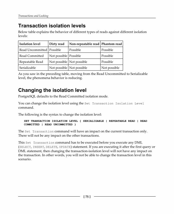
Transactions and Locking

[ 75 ]

Transaction isolation levelsBelow table explains the behavior of different types of reads against different isolationlevels:

Isolation level Dirty read Non-repeatable read Phantom read

Read Uncommitted Possible Possible Possible

Read Committed Not possible Possible Possible

Repeatable Read Not possible Not possible Possible

Serializable Not possible Not possible Not possible

As you saw in the preceding table, moving from the Read Uncommitted to Serializablelevel, the phenomena behavior is reducing.

Changing the isolation levelPostgreSQL defaults to the Read Committed isolation mode.

You can change the isolation level using the Set Transaction Isolation Levelcommand.

The following is the syntax to change the isolation level:

SET TRANSACTION ISOLATION LEVEL { SERIALIZABLE | REPEATABLE READ | READCOMMITTED | READ UNCOMMITTED }

The Set Transaction command will have an impact on the current transaction only.There will not be any impact on the other transactions.

This Set Transaction command has to be executed before you execute any DML(SELECT, INSERT, DELETE, UPDATE) statement. If you are executing it after the first query orDML statement, then changing the transaction-isolation level will not have any impact onthe transaction. In other words, you will not be able to change the transaction level in thisscenario.

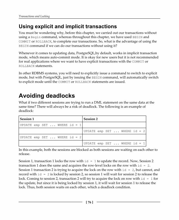
Transactions and Locking

[ 76 ]

Using explicit and implicit transactionsYou must be wondering why, before this chapter, we carried out our transactions withoutusing a Begin command, whereas throughout this chapter, we have used BEGIN andCOMMIT or ROLLBACK, to complete our transactions. So, what is the advantage of using theBEGIN command if we can do our transactions without using it?

Whenever it comes to updating data, PostgreSQL,by default, works in implicit transactionmode, which means auto-commit mode. It is okay for new users but it is not recommendedfor real applications where we want to have explicit transactions with the COMMIT orROLLBACK statements.

In other RDBMS systems, you will need to explicitly issue a command to switch to explicitmode, but with PostgreSQL, just by issuing the BEGIN command, will automatically switchto explicit mode until the COMMIT or ROLLBACK statements are issued.

Avoiding deadlocksWhat if two different sessions are trying to run a DML statement on the same data at thesame time? There will always be a risk of deadlock. The following is an example ofdeadlock:

Session 1 Session 2

UPDATE emp SET ... WHERE id = 1

UPDATE emp SET ... WHERE id = 2

UPDATE emp SET ... WHERE id = 2

UPDATE emp SET ... WHERE id = 1

In this example, both the sessions are blocked as both sessions are waiting on each other torelease.

Session 1, transaction 1 locks the row with id = 1 to update the record. Now, Session 2transaction 1 does the same and acquires the row-level locks on the row with id = 2.Session 1 transaction 2 is trying to acquire the lock on the row with id = 2, but cannot, andrecord with id = 2 is locked by session 2, so session 1 will wait for session 2 to release thelock. Coming to session 2, transaction 2 will try to acquire the lock on row with id = 1 forthe update, but since it is being locked by session 1, it will wait for session 1 to release thelock. Thus, both session waits on each other, which a deadlock condition.

Transactions and Locking

[ 77 ]

In this scenario, PostgreSQL will detect the deadlock and cancel one of the transactions.

There is no certainty which session PostgreSQL will choose to cancel, but it will try to pickthe one that it considers to have done the least work.

We should always develop our code in such a way that it should prevent deadlocks fromoccurring. One of the simplest techniques is to try and keep your transactions as short aspossible. The fewer records and tables involved in a transaction, the less time the locks willbe held and the less chance of deadlock. Another technique is to always process tables andrecords in the same order.

In the preceding example, if both sessions tried to update the rows in the same order, therewould not be a deadlock scenario. Session 1 would be able to update both its rows andcomplete, while Session 2 would wait till session 1 is complete. Explicit locking might beanother way to avoid the deadlock, which we will be covering in the next section.

Explicit lockingThere may come a time when you realize that the automatic locking PostgresSQL providesis not sufficient for your needs.

In order to fulfill your needs, you can explicitly lock the rows or, perhaps, an entire table.

In line with the SQL standards you will never see an option that will allow you to lock atable. One should only use explicit locking in urgent scenarios.

Locks for rows or tables are only allowed inside the transaction. Once the transaction getscompleted with a commit or rollback, all the locks acquired during the transaction will bereleased automatically.

An explicit lock cannot be released during the transaction because releasing the lock on arow that is being modified during a transaction might allow another application to changeit. This in turn will not allow the rollback to the initial changes.

Locking rowsDeadlocks can be avoided if we can lock the number of rows prior to making changes tothem. Locking rows prior to making the changes will allow you to restrict the changes thatwill be made by other applications—this will not allow the conflict part to happen.

Transactions and Locking

[ 78 ]

To lock a set of rows, we can use a SELECT statement and append a FOR UPDATE, as shownin the following example:

SELECT 1 FROM items WHERE unit_price > 15.0 FOR UPDATE;

This will lock all the rows in the items where the unit_price is greater than 15.0. As wedon't need any rows to be returned, we used 1 as a convenient way of minimizing the datareturned.

Consider the scenario where we want to lock all the rows in the employees table where theemployees live in Chicago because we need to change the telephone code, as the area codeis being split into several new ones. We will need to make sure that we can access all therows, but we will require some procedural code to then process each row in turn,calculating what the new telephone code should be.

=> BEGIN

BEGINbpfinal => SELECT customer_id FROM employees WHERE town = 'Chicago' FORUPDATE;

employee_id-------------48(2 rows)

The two rows with employee_id values 4 and 8 are locked, and we can test this by tryingto update them in a different psql session:

BEGIN=> UPDATE customer SET phone = '555-4444' WHERE employee_id = 4;UPDATE 1=> UPDATE customer SET phone = '555-8888' WHERE employee_id = 8;

At this point, the second session gets blocked until we press Ctrl + C to interrupt it, or thefirst session commits or rolls back.

At the beginning, the SELECT ... FOR UPDATE returns the rows with employee_ idvalues 4 and 8 to be locked. Other sessions are able to update different rows in theemployees table, but not rows 4 and 8 until the transaction is completed and the locks arereleased.

Transactions and Locking

[ 79 ]

Locking tablesPostgreSQL provides the functionality to lock the full table, although we don't recommendusing table lock if at all possible. You should comply with the other SQL standardmechanisms that ensure client isolation.

The syntax to lock tables is as follows:

LOCK [ TABLE ] table-nameLOCK [ TABLE ] table-name IN [ ROW | ACCESS ] { SHARE | EXCLUSIVE } MODELOCK [ TABLE ] table-name IN SHARE ROW EXCLUSIVE MODE

The simplest syntax that is used by the application generally is as follows:

LOCK TABLE table-name

This is the same as the following:

LOCK TABLE table-name ACCESS EXCLUSIVE MODE

This type of lock doesn't allow any application to access the table in any way. However, thistype of a lock is rarely used unless it is required in certain circumstances.

SummaryIn this chapter, we closely observed how transactions and locking work. We noticed how, ina single-user database, transactions are useful because they allow you to bind together SQLstatements in a single atomic unit. We also covered the multiuser environment for thetransactions. Then, we moved to the standard-isolation levels of ANSI SQL for theirundesirable phenomena and how we can eliminate different types of undesirable behaviorby defining various levels of transaction consistency. We also covered how we could end upwith performance degradation by eliminating desirable features. Therefore, it becomes veryessential to strike a balance between the ideal behavior and acceptable performance. Weexplored locking, and using simple techniques we can overcome the risk of deadlocks—asituation where two or more applications can freeze, waiting for the other to complete. Wealso did explicit locking, which provides the functionality to lock specific rows in a table orthe entire table within a transaction.

Transactions and Locking

[ 80 ]

However, transactions and locking do not directly modify data, which is what mostdatabase programmers really want to do. Understanding how these important features ofSQL work is critical to being able to write applications that safely use and update data in adatabase.

In the next chapter, we will discuss indexes and constraints, which will allow you tounderstand performance improvement techniques in a more interesting way.

6Indexes and Constraints

In the previous chapter, we talked about transactions and locking, which helped youunderstand their effect on the database. In this chapter, we will discuss indexes andconstraints, types of indexes and constraints, their use in the real world, and the bestpractices on when we need to and how to create them. Your application may have differentkinds of data, and you will want to maintain data integrity across the database and, at thesame time, you need a performance gain as well. This chapter helps you understand howyou can choose indexes and constraints for your requirement and improve performance. Italso covers real-time examples that will help you understand better. Of course, not all typesof indexes or constraints are the best fit for your requirement; however, you can choose therequired ones based on how they work.

Introduction to indexes and constraintsAn index is a pointer to the actual rows in its corresponding table. It is used to find andretrieve particular rows much faster than using the standard method. Indexes help youimprove the performance of queries. However, indexes get updated on every DataManipulation Language (DML)—that is, INSERT, UPDATE, and DELETE—query on thetable, which is an overhead, so they should be used carefully. Constraints are basically rulesrestricting the values allowed in the columns and they define certain properties that data ina database must comply with. The purpose of constraints is to maintain the integrity of datain the database. The different ways of maintaining data integrity through constraints will becovered in this chapter.

Indexes and Constraints

[ 82 ]

Primary key indexesAs the name indicates, primary key indexes are the primary way to identify a record (tuple)in a table. Obviously, it cannot be null because a null (unknown) value cannot be used toidentify a record. So, all RDBMSs prevent users from assigning a null value to the primarykey. The primary key index is used to maintain uniqueness in a column. You can have onlyone primary key index on a table. It can be declared on multiple columns.

In the real world, for example, if you take the empid column of the emp table, you will beable to see a primary key index on that as no two employees can have the same empidvalue.

You can add a primary key index in two ways: One is while creating the table and the other,once the table has been created.

This is how you can add a primary key while creating a table:

CREATE TABLE emp( empid integer PRIMARY KEY, empname varchar, sal numeric);

And this is how you can add a primary key after a table has been created:

CREATE TABLE emp( empid integer, empname varchar, sal numeric);

ALTER TABLE emp ADD PRIMARY KEY(empid);

Irrespective of whether a primary key is created while creating a table or after the table iscreated, a unique index will be created implicitly. You can check the unique index throughthe following command:

postgres=# select * from pg_indexes where tablename='emp';-[ RECORD 1 ]-----------------------------------------------------schemaname | publictablename | empindexname | emp_pkeytablespace |indexdef | CREATE UNIQUE INDEX emp_pkey ON emp USING btree (empid)

Indexes and Constraints

[ 83 ]

Since it maintains uniqueness in the column, what happens if you try to INSERT a duplicaterow or NULL values? Let's check it out:

postgres=# INSERT INTO emp VALUES(100, 'SCOTT', '10000.00');INSERT 0 1postgres=# INSERT INTO emp VALUES(100, 'ROBERT', '20000.00');ERROR: duplicate key value violates unique constraint "emp_pkey"DETAIL: Key (empid)=(100) already exists.postgres=# INSERT INTO emp VALUES(null, 'ROBERT', '20000.00');ERROR: null value in column "empid" violates not-null constraintDETAIL: Failing row contains (null, ROBERT, 20000).

So, if empid is a duplicate value, the database throws an error; duplicate keyviolation due to unique constraint; if empid is null, the error is violates null constraintdue to not-null constraint. A primary key is simply a combination of a unique and a not-null constraint.

Unique indexesLike a primary key index, a unique index is also used to maintain uniqueness; however, itallows NULL values. The syntax is as follows:

CREATE TABLE emp( empid integer UNIQUE, empname varchar, sal numeric);

CREATE TABLE emp( empid integer, empname varchar, sal numeric, UNIQUE(empid));

This is what happens if you INSERT NULL values:

postgres=# INSERT INTO emp VALUES(100, 'SCOTT', '10000.00');INSERT 0 1postgres=# INSERT INTO emp VALUES(null, 'SCOTT', '10000.00');INSERT 0 1postgres=# INSERT INTO emp VALUES(null, 'SCOTT', '10000.00');INSERT 0 1

As you see, it allows NULL values, and they are not even considered as duplicate values.

Indexes and Constraints

[ 84 ]

If a unique index is created on a column then there is no need for astandard index on the column. If you had one, it would just be a duplicateof the automatically created index. Currently, only B-tree indexes can bedeclared unique.

When a primary key is defined, PostgreSQL automatically creates a unique index. You cancheck it out using the following query:

postgres=# select * from pg_indexes where tablename ='emp';-[ RECORD 1 ]-----------------------------------------------------schemaname | publictablename | empindexname | emp_empid_keytablespace |indexdef | CREATE UNIQUE INDEX emp_empid_key ON emp USING btree(empid)

B-tree indexesLike most relational databases, PostgreSQL also supports B-tree indexes. Most RDBMSsystems use B-tree as the default index type, unless something else is specified explicitly.Basically, this index keeps data stored in a tree (self-balancing) structure. It's the defaultindex in PostgreSQL and fits in the most common situations.

The B-tree index can be used by an optimizer whenever the indexed column is used with acomparison operator, such as <, <=, =, >=, >, and LIKE or the ~ operator; however, LIKE or~ will only be used if the pattern is a constant and anchored to the beginning of the string,for example, my_col LIKE 'mystring%' or my_column ~ '^mystring', but notmy_column LIKE '%mystring'.

Here is an example:

CREATE TABLE emp( empid integer, empname varchar, sal numeric);

INSERT INTO emp VALUES(100, 'scott', '10000.00');

INSERT INTO emp VALUES(100, 'clark', '20000.00');

INSERT INTO emp VALUES(100, 'david', '30000.00');

INSERT INTO emp VALUES(100, 'hans', '40000.00');

Indexes and Constraints

[ 85 ]

Create a B-tree index on the empname column:

CREATE INDEX emp_empid_idx ON emp(empid);CREATE INDEX emp_name_idx ON emp(empname);

Here are the queries that use index:

postgres=# explain analyze SELECT * FROM emp WHERE empid=100; QUERY PLAN---------------------------------------------------------------Index Scan using emp_empid_idx on emp (cost=0.13..4.15 rows=1 width=68)(actual time=1.015..1.304 rows=4 loops=1)Index Cond: (empid = 100)Planning time: 0.496 msExecution time: 2.096 mspostgres=# explain analyze SELECT * FROM emp WHERE empname LIKE 'da%'; QUERY PLAN----------------------------------------------------------------Index Scan using emp_name_idx on emp (cost=0.13..4.15 rows=1 width=68)(actual time=0.956..0.959 rows=1 loops=1)Index Cond: (((empname)::text >= 'david'::text) AND ((empname)::text <'david'::text))Filter: ((empname)::text ~~ 'david%'::text)Planning time: 2.285 msExecution time: 0.998 ms

Here is a query that cannot use index as % is used at the beginning of the string:

postgres=# explain analyze SELECT * FROM emp WHERE empname LIKE '%david'; QUERY PLAN----------------------------------------------------------------Seq Scan on emp (cost=10000000000.00..10000000001.05 rows=1 width=68)(actual time=0.014..0.015 rows=1 loops=1)Filter: ((empname)::text ~~ '%david'::text)Rows Removed by Filter: 3Planning time: 0.099 msExecution time: 0.044 ms

Standard indexesIndexes are primarily used to enhance database performance (though incorrect use canresult in slower performance). An index can be created on multiple columns and multipleindexes can be created on one table. The syntax is as follows:

CREATE [ UNIQUE ] INDEX [ CONCURRENTLY ] [ name ] ON table_name [ USINGmethod ]

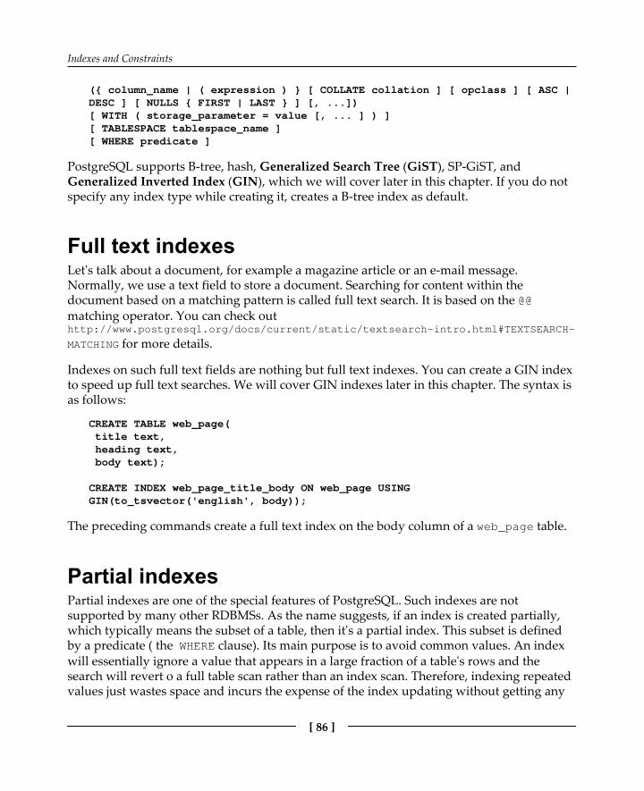
Indexes and Constraints

[ 86 ]

({ column_name | ( expression ) } [ COLLATE collation ] [ opclass ] [ ASC |DESC ] [ NULLS { FIRST | LAST } ] [, ...])[ WITH ( storage_parameter = value [, ... ] ) ][ TABLESPACE tablespace_name ][ WHERE predicate ]

PostgreSQL supports B-tree, hash, Generalized Search Tree (GiST), SP-GiST, and Generalized Inverted Index (GIN), which we will cover later in this chapter. If you do notspecify any index type while creating it, creates a B-tree index as default.

Full text indexesLet's talk about a document, for example a magazine article or an e-mail message.Normally, we use a text field to store a document. Searching for content within thedocument based on a matching pattern is called full text search. It is based on the @@matching operator. You can check outhttp://www.postgresql.org/docs/current/static/textsearch-intro.html#TEXTSEARCH-

MATCHING for more details.

Indexes on such full text fields are nothing but full text indexes. You can create a GIN indexto speed up full text searches. We will cover GIN indexes later in this chapter. The syntax isas follows:

CREATE TABLE web_page( title text, heading text, body text);

CREATE INDEX web_page_title_body ON web_page USINGGIN(to_tsvector('english', body));

The preceding commands create a full text index on the body column of a web_page table.

Partial indexesPartial indexes are one of the special features of PostgreSQL. Such indexes are notsupported by many other RDBMSs. As the name suggests, if an index is created partially,which typically means the subset of a table, then it's a partial index. This subset is definedby a predicate ( the WHERE clause). Its main purpose is to avoid common values. An indexwill essentially ignore a value that appears in a large fraction of a table's rows and thesearch will revert o a full table scan rather than an index scan. Therefore, indexing repeatedvalues just wastes space and incurs the expense of the index updating without getting any

Indexes and Constraints

[ 87 ]

performance benefit back at read time. So, common values should be avoided.

Let's take a common example, an emp table. Suppose you have a status column in an emptable that shows whether emp exists or not. In any case, you care about the currentemployees of an organization. In such cases, you can create a partial index in the statuscolumn by avoiding former employees.

Here is an example:

CREATE TABLE emp_table empid integer, empname varchar, status varchar);

INSERT INTO emp_table VALUES(100, 'scott', 'exists');

INSERT INTO emp_table VALUES(100, 'clark', 'exists');

INSERT INTO emp_table VALUES(100, 'david', 'not exists');

INSERT INTO emp_table VALUES(100, 'hans', 'not exists');

To create a partial index that suits our example, we will use the following query

CREATE INDEX emp_table_status_idx ON emp_table(status) WHERE status NOTIN('not exists');

Now, let's check the queries that can use the index and those that cannot.

A query that uses the index is as follows:

postgres=# explain analyze select * from emp_table where status='exists'; QUERY PLAN-------------------------------------------------------------------Index Scan using emp_table_status_idx on emp_table(cost=0.13..6.16 rows=2width=17) (actual time=0.073..0.075 rows=2 loops=1)Index Cond: ((status)::text = 'exists'::text)

A query that will not use the index is as follows:

postgres=# explain analyze select * from emp_table wherestatus='not exists'; QUERY PLAN----------------------------------------------------------------Seq Scan on emp_table (cost=10000000000.00..10000000001.05 rows=1 width=17)(actual time=0.013..0.014 rows=1 loops=1)Filter: ((status)::text = 'not exists'::text)Rows Removed by Filter: 3

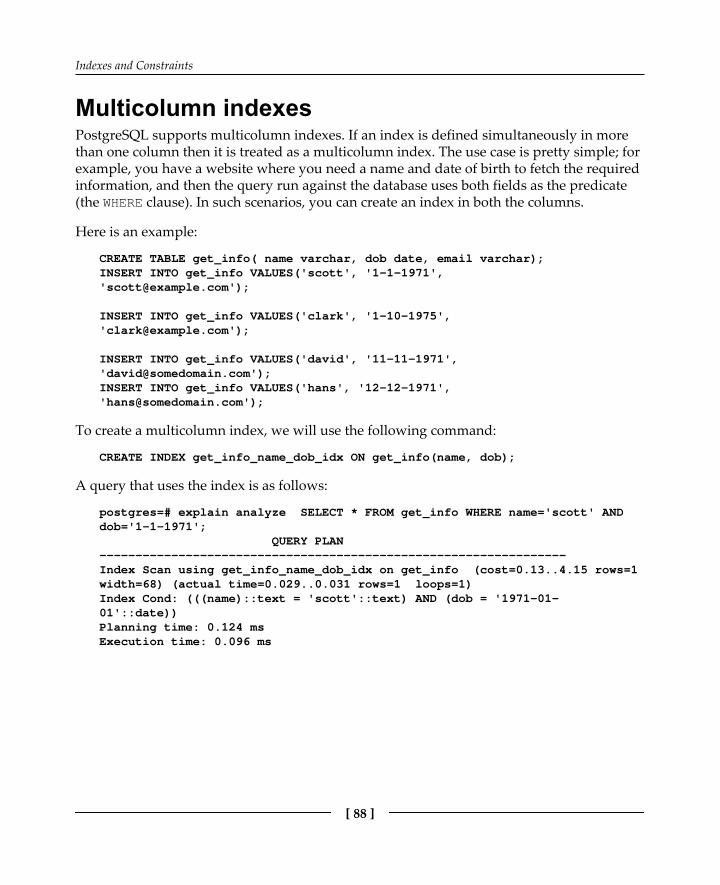
Indexes and Constraints

[ 88 ]

Multicolumn indexesPostgreSQL supports multicolumn indexes. If an index is defined simultaneously in morethan one column then it is treated as a multicolumn index. The use case is pretty simple; forexample, you have a website where you need a name and date of birth to fetch the requiredinformation, and then the query run against the database uses both fields as the predicate(the WHERE clause). In such scenarios, you can create an index in both the columns.

Here is an example:

CREATE TABLE get_info( name varchar, dob date, email varchar);INSERT INTO get_info VALUES('scott', '1-1-1971','scott@example.com');

INSERT INTO get_info VALUES('clark', '1-10-1975','clark@example.com');

INSERT INTO get_info VALUES('david', '11-11-1971','david@somedomain.com');INSERT INTO get_info VALUES('hans', '12-12-1971','hans@somedomain.com');

To create a multicolumn index, we will use the following command:

CREATE INDEX get_info_name_dob_idx ON get_info(name, dob);

A query that uses the index is as follows:

postgres=# explain analyze SELECT * FROM get_info WHERE name='scott' ANDdob='1-1-1971'; QUERY PLAN-----------------------------------------------------------------Index Scan using get_info_name_dob_idx on get_info (cost=0.13..4.15 rows=1width=68) (actual time=0.029..0.031 rows=1 loops=1)Index Cond: (((name)::text = 'scott'::text) AND (dob = '1971-01-01'::date))Planning time: 0.124 msExecution time: 0.096 ms

Indexes and Constraints

[ 89 ]

Hash indexesThese indexes can only be used with equality comparisons. So, an optimizer will considerusing this index whenever an indexed column is used with the = operator.

Here is the syntax:

CREATE INDEX index_name ON table USING HASH (column);

Hash indexes are faster than B-tree as they should be used if the column in question is neverintended to be scanned comparatively with < or > operators.

The Hash indexes are not WAL-logged, so they might need to be rebuiltafter a database crash, if there were any unwritten changes.

GIN and GiST indexesGIN or GiST indexes are used for full text searches. GIN can only be created on thetsvector datatype columns and GIST on tsvector or tsquery database columns. Thesyntax is follows:

CREATE INDEX index_name ON table_name USING GIN (column_name);CREATE INDEX index_name ON table_name USING GIST (column_name);

These indexes are useful when a column is queried for specific substrings on a regular basis;however, these are not mandatory.

What is the use case and when do we really need it? Let me give an example to explain.Suppose we have a requirement to implement simple search functionality for anapplication. Say, for example, we have to search through all users in the database. Also, let'sassume that we have more than 10 million users currently stored in the database.

This search implementation requirement shows that we should be able to search usingpartial matches and multiple columns, for example, first_name, last_name. Moreprecisely, if we have customers like Mitchell Johnson and John Smith, an input query ofJohn should return for both customers. We can solve this problem using the GIN or GISTindexes.

Here is an example:

CREATE TABLE customers (first_name text, last_name text);Create GIN/GiST index:

Indexes and Constraints

[ 90 ]

CREATE EXTENSION IF NOT EXISTS pg_trgm;CREATE INDEX customers_search_idx_gin ON customers USING gin (first_namegin_trgm_ops, last_name gin_trgm_ops);CREATE INDEX customers_search_idx_gist ON customers USING gist (first_namegist_trgm_ops, last_name gist_trgm_ops);

So, what is the difference between these two indexes? This is what the PostgreSQLdocumentation says:

GiST is faster to update and build the index and is less accurate than GIN

GIN is slower to update and build the index but is more accurate. According to thedocumentation, the GiST index is lossy. This means that the index might produce falsematches, and it is necessary to check the actual table row to eliminate such false matches(PostgreSQL does this automatically when needed).

Block Range Index (BRIN) indexes were introduced in PostgreSQL 9.5. BRIN indexes aredesigned to handle very large tables in which certain columns have some naturalcorrelation with their physical location within the table. The syntax is follows:

CREATE INDEX index_name ON table_name USING brin(col);

Here is a good example: h t t p s : / / w i k i . p o s t g r e s q l . o r g / w i k i / W h a t % 2 7 s _ n e w _ i n _ P o s t g r e

S Q L _ 9 . 5 # B R I N _ I n d e x e s.

Clustering on an indexPostgreSQL supports clustering a table using an index. CLUSTER is used to do that. Whatdoes it do? It reorganizes the table based on the index. Why do we need it? It can greatlyincrease performance when you query a range of index values or a single index value withmultiple entries because the queried data is in one place on the disk.

The syntax is as follows:

CLUSTER [VERBOSE] table_name [ USING index_name ]

Here's an example of how to create a cluster and how it improves the performance:

CREATE TABLE table_cluster( id integer, name varchar);INSERT INTO table_cluster VALUES(generate_series(1,10000000),'test_name'||generate_series(1,10000000));CREATE INDEX table_cluster_idx ON table_cluster(id);

Indexes and Constraints

[ 91 ]

Query the table in such way that the index is used and look at the execution time. Thefollowing is an example:

postgres=# EXPLAIN ANALYZE SELECT * FROM table_cluster WHERE id BETWEEN10000 AND 200000; QUERY PLAN-----------------------------------------------------------------Index Scan using table_cluster_idx on table_cluster (cost=0.43..44955.39rows=855991 width=19) (actual time=1.741..535.026 rows=760004 loops=1)Index Cond: ((id >= 10000) AND (id <= 200000))Planning time: 5.241 msExecution time: 572.737 ms

Now, CLUSTER the table using index and query the table:

postgres=# CLUSTER table_cluster USING table_cluster_idx;CLUSTERpostgres=# EXPLAIN ANALYZE SELECT * FROM table_cluster WHERE idBETWEEN 10000 AND 200000 QUERY PLAN-------------------------------------------------------------------Index Scan using table_cluster_idx on table_cluster (cost=0.43..44955.39rows=855991 width=19) (actual time=1.777..272.387 rows=760004 loops=1)Index Cond: ((id >= 10000) AND (id <= 200000))Planning time: 0.283 msExecution time: 310.143 ms

If you can see, the query execution time reduced to almost 40%.

Keep in mind that the CLUSTER operation takes an ACCESS EXCLUSIVElock on the table, which typically means that it does not allow any otheroperation on the table while CLUSTER is running.

Foreign key constraintsForeign key constraints maintain referential integrity between two related tables. Theyspecify that values in a column of a table must match with some rows of another table.

Let's take one common example of the emp and dept table. We have to make sure that theemp table contains only valid deptno values, that can be found in the dept table:

CREATE TABLE dept( deptno numeric PRIMARY KEY, dname varchar, loc varchar);

Indexes and Constraints

[ 92 ]

CREATE TABLE emp( empno numeric PRIMARY KEY, ename varchar, job varchar, mgr numeric, hiredate date, sal numeric, comm numeric, deptno numeric(2,0), constraint fk_deptno foreign key (deptno) references dept (deptno));

Let's try to INSERT some data in the emp table for which deptno does not exist in the depttable:

INSERT INTO dept VALUES(10, 'ACCOUNTING', 'NEW YORK'); INSERT INTO dept VALUES(20, 'RESEARCH', 'DALLAS');

We have a couple of deptno (10 and 20) in the dept table. As the foreign key constraintmaintains referential integrity, it should not allow any deptno in the emp table other than10 and 20. Let's try it using the following command:

INSERT INTO emp VALUES(7782, 'CLARK', 'MANAGER', 7839,to_date('9-6-1981','dd-mm-yyyy'),2450, null, 40);ERROR: insert or update on table "emp" violates foreign key constraint"fk_deptno" DETAIL: Key (deptno)=(40) is not present in table "dept".

It clearly throws an ERROR that, as deptno 40 is not in the dept table, it cannot be insertedin the emp table as well. In this way, we can maintain referential integrity by creatingforeign key constraints.

Unique constraintsWe create unique constraints to make sure that data contained in a column is unique amongall rows in the table. The syntax is as follows:

CREATE TABLE example_1( col1 integer, col2 integer, col3 integer, UNIQUE(col1) );

It can be created on a group of columns as well. The syntax is as follows:

CREATE TABLE example_2( col1 integer,

Indexes and Constraints

[ 93 ]

col2 integer, col3 integer, UNIQUE(col1, col2));

You can define a unique constraint even after the table is created, as shown in the followingcommand:

ALTER TABLE example ADD CONSTRAINT example_col1_unique UNIQUE(col1);

Adding this constraint will automatically create a B-tree index on the column.

Please note that two null values are never considered equal in thiscomparison. That means though a unique constraint is defined, it ispossible to store duplicate rows that contain a null value in at least one ofthe constrained columns. So, be careful when developing applications thatare intended to be portable.

Now, let's try to insert duplicate values and see what error it throws:

INSERT INTO example_1 VALUES(1,2,1);

postgres=# INSERT INTO example postgres-# VALUES(1,2,1); ERROR: duplicate key value violates unique constraint "example_col1_key" DETAIL: Key (col1)=(1) already exists.

So, it clearly says, values already exist and cannot be inserted again. However, try insertingNULL values and see what happens:

postgres=# INSERT INTO examplepostgres-# VALUES(null,1,1);INSERT 0 1

postgres=# INSERT INTO examplepostgres-# VALUES(null,1,1);INSERT 0 1

postgres=# select * from example ;col1 | col2 | col3------+------+------| 1 | 1| 1 | 1(2 rows)

So, as noted in the preceding example, a unique constraint does not consider null values asduplicates.

Indexes and Constraints

[ 94 ]

Check constraintsCheck constraints allow you to specify that the value in a certain column must satisfy aBoolean (truth-value) expression. We use the CHECK keyword to define it. The syntax is asfollows:

CREATE TABLE products( name varchar, product varchar, product_price numeric CHECK (product_price > 0));

In the preceding example, it makes sure that product_price is greater than 0. Theprevious example is a default value definition and a name will be given by the system;however, you can create check constraints with a separate name that clarifies errormessages and allows you to refer to the constraint when you need to change it. Here is anexample:

CREATE TABLE products( name varchar, product varchar, product_price numeric CONSTRAINT product_price_check CHECK (product_price > 1));

In the preceding definition, product_price_check is the name of the check constraint.

We can also define check constraints at table level, which is slightly different from columnlevel. Here is an example:

CREATE TABLE products( name varchar, product varchar, product_price numeric CHECK (product_price > 0), discount_price numeric, CONSTRAINT discount_price_check CHECK (product_price > discount_price));

Let's test the check constraint by inserting some data:

INSERT INTO products VALUES('Pen', 'Stationary', '100.00', 0);INSERT INTO products VALUES('Pen', 'Stationary', '-100.00',0);

ERROR: new row for relation "products" violates check constraint"products_check"DETAIL: Failing row contains (Pen, Stationary, -100.00, 0).

Indexes and Constraints

[ 95 ]

As per the column, the check constraint throws an error. However, it also has a table levelconstraint; let's check it by inserting some data:

INSERT INTO products VALUES('Pen', 'Stationary', '100.00', '200.00');ERROR: new row for relation "products" violates check constraint"discount_price_check"DETAIL: Failing row contains (Pen, Stationary, 100.00, 200.00).

If you look at the error, it clearly shows it is due to the "discount_price_check"constraint, which is defined at the table level.

NOT NULL constraintsAs the name suggests, NOT NULL constraint simply specifies that a null value is notallowed. Let's take a look at an example:

CREATE TABLE products( name varchar, product varchar, product_price NOT NULL);

Let's test this constraint by inserting a null value:

INSERT INTO products VALUES('Pen', 'Stationary', null);ERROR: null value in column "product_price" violates not-null constraintDETAIL: Failing row contains (Pen, Stationary, null).

PostgreSQL also supports NULL constraints. They should not be used in portableapplications and are there for just compatibility as some other database systems have this.Here's an example:

CREATE TABLE products( name varchar NULL, product varchar, product_price integer NULL);

Indexes and Constraints

[ 96 ]

Exclusion constraintsThis constraint specifies that if any two rows are compared on the specified column(s) orexpression(s) using the specified operator(s), at least one of these operator comparisons willreturn false or null. Let's look at this example:

CREATE EXTENSION btree_gist;CREATE TABLE example( name varchar, age integer, EXCLUDE USING gist (AGE WITH <>));

In the preceding example, we are enforcing that age has to match an already existing one.What happens if you try to insert a different age? Let's look at this example:

postgres=# INSERT INTO example VALUES ('scott', '26');INSERT 0 1postgres=# INSERT INTO example VALUES ('scott', '27');ERROR: conflicting key value violates exclusion constraint"example_age_excl"DETAIL: Key (age)=(27) conflicts with existing key (age)=(26).

It throws an ERROR that the exclusion constraint is violated. Adding an exclusion constraintwill automatically create an index of the type specified in the constraint declaration.

SummaryIn this chapter, we looked at different types of indexes and constraints that PostgreSQLsupports, how they are used in the real world with examples, and what happens if youviolate a constraint. It not only helps you identify the right index for your data, but alsoimproves the performance of the database. Every type of index or constraint has its ownidentification and need. Some indexes or constraints may not be portable to other RDBMSs,some may not be needed, or sometimes you might have chosen the wrong one for yourneeds. So be careful to choose the right one from which you get the benefit and one whichsatisfies your exact needs. In the next chapter, we will talk about the benefits of tablepartitioning in PostgreSQL and how to implement them. We will also cover managingpartitions and alternate partitioning options.

7Table Partitioning

In the last chapter, we talked about indexes and constraints in detail. It helped you tounderstand the purpose of indexes/constraints, and the best way we can use them in thereal world. In this chapter, we are going to talk about table partitioning. We'll start with abasic introduction to partitioning, and will cover topics such as need for partitioning, theway it is done, and how exactly it helps. We will also discuss about the flow, that is, how itworks so that you can have better control over it. You will learn how to manage tablepartitions once they are created, the kind of maintenance they require, and how to make thesystem get the best use out of it. We will also talk about types of partitioning thatPostgreSQL supports, and alternative methods of partitioning. We will also discuss theimpact if you do not partition a table.

Table partitioningPartitioning is a feature in DBMS which segregates large amounts of data into multiplesegments based on an attribute of a relation. Using this as a feature, we can performoperations effectively on large datasets. We can also go without partitioning the largedatasets, but eventually we'll need to pay for performance as a result. The query responsetime and the amount of data it processes are inversely proportional. So, in short, the moredata we have, the less performance we get (where performance is the actual time of queryexecution).

For example, consider we have a global business where we store all our global customers'information in our local database as follows:

CREATE TABLE customers(id integer,name varchar(126),countrycode varchar(3),contactnum text);

Table Partitioning

[ 98 ]

In the preceding table, we will store all our global customer details along with thecountrycode. For demonstration purposes, I am going to use three-character countrynames, which are generated randomly from the following query:

postgres=# WITH stuff AS ( SELECT array['A', 'B', 'C', 'D', 'E', 'F', 'G', 'H'] as names, array['USA', 'UK', 'UAE', 'IND', 'GER', 'RUS'] AS cnames) INSERT INTO customers SELECT Generate_series(1, 1000) id, names[(random()*100)::int%8+1] cname, cnames[(random()*100)::int%6+1] countrycode, ltrim(round(random()::numeric, 10)::text, '0.') contactnumber FROM stuff; INSERT 0 1000

In the preceding query, we took an array of customer and country names, which we aregoing to choose randomly to populate into our customers table; we then populated ourtable with 1000 entries. As an ad hoc reporting request, let's assume that we need to countthe number of customers we have in 'USA', 'UK', and 'IND'. Here is the query for therequest:

We enable timing at psql client, which gives us the total query execution followed by thequery result.

postgres=# \timingTiming is on.postgres=# SELECT COUNT(*), countrycode FROM customers WHERE countrycode IN('USA', 'UK', 'IND') GROUP BY countrycode;count | countrycode------+------- 167 | UK 171 | IND 154 | USATime: 9.202 ms

From the preceding result, we see that the query execution takes 9.202 ms to operate on1000 records. Let's push more records into the table, and see the response time. In thefollowing request, I push 10 times the current record count.

Now, let's execute our ad hoc request, and see the response time.

postgres=# SELECT COUNT(*), countrycode FROM customers WHERE countrycodeIN ('USA', 'UK', 'IND') GROUP BY countrycode;count | countrycode------+-------

Table Partitioning

[ 99 ]

1858 | UK 1810 | IND 1930 | UAETime: 9.661 ms

From the preceding results, it seems we paid 0.459 ms extra time for the same query, on alarge dataset. Let's increase the dataset by 10 times the current record count, and see theresponse time for the same query:

postgres=# SELECT COUNT(*), countrycode FROM customers WHERE countrycodeIN ('USA', 'UK', 'IND') GROUP BY countrycode;count | countrycode------+---------16962 | UK16382 | USA16925 | IND(3 rows)Time: 70.994 ms

From the preceding examples, we can see that the query response time is inverselyproportional to the dataset. So first let's try to optimize the query, which will improve thequery response time without using the partition.

Let's look at the query execution plan:

postgres=# EXPLAIN ANALYZE SELECT COUNT(*), countrycode FROM customersWHERE countrycode IN ('USA', 'UK', 'IND') GROUP BY countrycode; QUERY PLAN--------------------------------------------------------------HashAggregate (cost=2262.65..2262.69 rows=4 width=3) (actualtime=78.162..78.163 rows=3 loops=1)Group Key: countrycode-> Seq Scan on customers (cost=0.00..2012.00 rows=50130 width=3) (actualtime=0.017..50.113 rows=50269 loops=1)Filter: ((countrycode)::text = ANY ('{USA,UK,IND}'::text[]))Rows Removed by Filter: 49731Planning time: 0.195 msExecution time: 78.227 ms(7 rows)Time: 79.157 ms

From the preceding plan, we see that our predicate column (countrycode) is not indexed.That is the reason it went for a sequential scan. Let's create an index and see the plan:

postgres=# CREATE INDEX CONCURRENTLY countrycode_idx ONcustomers(countrycode);CREATE INDEXTime: 390.520 ms

Table Partitioning

[ 100 ]

postgres=# EXPLAIN ANALYZE SELECT COUNT(*), countrycode FROM customersWHERE countrycode IN ('USA', 'UK', 'IND') GROUP BY countrycode; QUERY PLAN-------------------------------------------------------------HashAggregate (cost=2262.65..2262.69 rows=4 width=3) (actualtime=74.823..74.823 rows=3 loops=1)Group Key: countrycode-> Seq Scan on customers (cost=0.00..2012.00 rows=50130 width=3) (actualtime=0.018..47.365 rows=50269 loops=1)Filter: ((countrycode)::text = ANY ('{USA,UK,IND}'::text[]))Rows Removed by Filter: 49731Planning time: 0.378 msExecution time: 74.883 ms(7 rows)Time: 75.866 ms

It seems our assumption is incorrect. Even after creating the index on the required predicatecolumn, our query still takes the sequential scan. This is the expected behavior when aquery tries to fetch more than 50% of the table;the optimizer skips the index scan in thatcase. If you observe the previous execution plan, we see rows=50269, which is 50% of theactual table count. That is the reason our index did not get picked up. Here I inserted sixcountry codes randomly, out of which I selected three country codes. It means that weselected 50% of the actual table.

So let's try to eliminate one countrycode from the predicate, and see if the plan takes thecreated index:

postgres=# EXPLAIN ANALYZE SELECT COUNT(*), countrycode FROM customersWHERE countrycode IN ('USA', 'UK') GROUP BY countrycode; QUERY PLAN-------------------------------------------------------------HashAggregate (cost=1794.58..1794.60 rows=2 width=3) (actualtime=39.266..39.267 rows=2 loops=1)Group Key: countrycode-> Bitmap Heap Scan on customers (cost=574.71..1628.04 rows=33307width=3) (actual time=11.880..20.284 rows=33344 loops=1)Recheck Cond: ((countrycode)::text = ANY ('{USA,UK}'::text[]))Heap Blocks: exact=637-> Bitmap Index Scan on countrycode_idx (cost=0.00..566.38 rows=33307width=0) (actual time=11.724..11.724 rows=33344 loops=1)Index Cond: ((countrycode)::text = ANY ('{USA,UK}'::text[]))Planning time: 0.167 msExecution time: 39.343 ms(9 rows)Time: 40.007 ms

Table Partitioning

[ 101 ]

Yeah, now it works. Moreover, we reduced the query response time to half by creating theindex on the required predicate column. Here the query fetches less than 50% of the actualrecord set.

In the preceding example, we reduced the query response time to some extent by creatingthe required index. However, our global business will not stop with a certain number ofclients. Business needs to scale and get more customers. So let's insert more records into thecustomers table, and see the query response time.

postgres=# SELECT COUNT(*) FROM customers;count---------3000000(1 row)Time: 926.910 mspostgres=# EXPLAIN ANALYZE SELECT COUNT(*), countrycode FROM customersWHERE countrycode IN ('USA', 'UK') GROUP BY countrycode; QUERY PLAN------------------------------------------------------------------GroupAggregate (cost=0.43..106932.53 rows=3 width=3) (actualtime=492.174..930.943 rows=2 loops=1)Group Key: countrycode-> Index Only Scan using countrycode_idx on customers(cost=0.43..101860.00 rows=1014500 width=3) (actual time=0.117..697.074rows=1004893 loops=1)Index Cond: (countrycode = ANY ('{USA,UK}'::text[]))Heap Fetches: 1004893Planning time: 0.350 msExecution time: 931.001 ms(7 rows)Time: 932.133 ms

In the preceding example, the index scan helps us to reduce the query response time.However, if the table keeps on growing like this, even index scans might not help us after acertain point.

So what is the best solution to handle this kind of large data sets? As of now, the solution toachieve better performance is partitioning. You might wonder, “How do we partition atable, and how we can manage the partitions?”. Let's discuss this in more detail.

Table Partitioning

[ 102 ]

Partition implementationWhat does actually happen when we implement partitions on any table?

Does Postgres create a different storage for the partition?Is this partition object similar to objects like an index or a view?Is this a mechanism that internally segregates table data into multiple chunks?

To answer all these questions, partitioning a table is nothing but creating a separate tablecalled a child table for each partition. Child tables do not have any special characteristics, asthey are completely similar to normal tables. The original table on which we create apartition is called the parent table. Let's see more details about parent and child tables infurther discussions.

Before implementing partitions on any table, we have to take a decision on which column ofthe table we need to create partitions. Also, we need to understand the column's data typetoo.

So how to choose a column for partitioning?

In our table structure, we have columns like id, name, countrycode, and contactnum.And we need to choose a column on which to a create partition, which will improve ourquery response time. In general, we need to choose a column whose values are morerepetitive than any other column. For example, the id, name, and contactnum columns willhave fewer repetitive values than countrycode. And the data type of the countrycode istext.

As I mentioned earlier, before creating any partition we need to choose a proper column inthe table along with its data type. Here, we chose countrycode as our partitioning columnsince it has more duplicate values than other columns.

So, we are finally ready to do partitioning of a table. As mentioned previously, we need tocreate partitions on the parent table.

So, let's create a parent table first, and then will create child (partition) tables:

postgres=# CREATE TABLE IF NOT EXISTS customers(id int, name varchar(126),countrycode varchar(3),contactnum text);

You might've noticed that the syntax for creation of a parent table is similar to that of ourregular tables. Yes, you are correct. Regular tables become parent tables when we partitionthem.

Table Partitioning

[ 103 ]

Now, let's create child tables for the parent table, and partition the table on each countrycode. We have six country codes, so create one child table for each country code in theparent table, which will be six in total, and suffix the country code to the table name foreasy understanding.

This is done as follows:

CREATE TABLE customers_USA(CHECK (countrycode='USA')) INHERITS(customers);CREATE TABLE customers_UK(CHECK (countrycode='UK')) INHERITS(customers);CREATE TABLE customers_UAE(CHECK (countrycode='UAE')) INHERITS(customers);CREATE TABLE customers_IND(CHECK (countrycode='IND')) INHERITS(customers);CREATE TABLE customers_GER(CHECK (countrycode='GER')) INHERITS(customers);CREATE TABLE customers_RUS(CHECK (countrycode='RUS')) INHERITS(customers);

Now look at the difference in syntax for creation of the child tables. While creating the childtables, we have used the INHERITS table feature, which will automatically inherit the giventable's columns along with its modifiers like not null, and default properties.

Also, we have added an additional data consistency CHECK constraint, which makes surethat the created child table will only allow the respective country code values.

We can use psql's meta command(\d+) to see all the child tables of a partitioned table, asfollows:

postgres=# \d+ customersTable "public.customers"Column | Type | Modifiers | Storage | Stats target | Description-------+------+-----------+---------+--------------+-------------id | integer | | plain | |name | character varying(126) | | extended | |countrycode | character varying(3) | | extended | |contactnum | text | | extended | |Child tables: customers_ger,customers_ind,customers_rus,customers_uae,customers_uk,customers_usa

Or, we can also use pg_inherits table, to get a child's information:

postgres=# SELECT inhrelid::regclass, inhparent::regclass from pg_inheritsWHERE inhparent::regclass='customers'::regclass; inhrelid | inhparent--------------+-----------customers_usa | customerscustomers_uk | customers

Table Partitioning

[ 104 ]

customers_uae | customerscustomers_ind | customerscustomers_ger | customerscustomers_rus | customers

Now, you might have another question like “How is my application going to communicatewith the child tables?” Actually, your application has no need to know what all the childtables for the given partitioned table are, as your application only deals with the parenttable.

All application DML operations will be diverted to the corresponding child table with thehelp of the INHERITS feature along with the before insert trigger on the parent table.

So let's create a before insert trigger on the parent table, and see how the parent tablehandles the incoming DML operations:

CREATE OR REPLACE FUNCTION customers_before_insert_trig_func() RETURNStrigger AS$$BEGIN

IF (NEW.countrycode='USA') THEN INSERT INTO customers_usa VALUES(NEW.*);ELSIF (NEW.countrycode='UK') THEN INSERT INTO customers_uk VALUES(NEW.*);ELSIF (NEW.countrycode='IND') THEN INSERT INTO customers_ind VALUES(NEW.*);ELSIF (NEW.countrycode='GER') THEN INSERT INTO customers_GER VALUES(NEW.*);ELSIF (NEW.countrycode='UAE') THEN INSERT INTO customers_uae VALUES(NEW.*);ELSIF (NEW.countrycode='RUS') THEN INSERT INTO customers_rus VALUES(NEW.*);ELSE --Unknown country code, we got as an input. --Here, we can either RAISE ERROR or --We can store the unknown country code on some other child table RAISE EXCEPTION 'Unknown country code we got';END IF;RETURN NULL;END;$$ LANGUAGE PLPGSQL;

CREATE TRIGGER customers_ins_trig before INSERT ON customers FOR each rowEXECUTE PROCEDUREcustomers_before_insert_trig_func();

Table Partitioning

[ 105 ]

From the preceding trigger function, we can see that an explicit INSERT operation ishappening on the corresponding child table, based on the country codes. In this way, wecan handle our INSERT operation on the parent table.

Now let's insert a few random records, and see how it goes:

postgres=# WITH stuff AS( SELECT array['A', 'B', 'C', 'D', 'E', 'F', 'G', 'H'] as names, array['USA', 'UK', 'UAE', 'IND', 'GER', 'RUS'] AS cnames)INSERT INTO customersSELECT Generate_series(1, 1000) id,names[(random()*100)::int%8+1] cname,cnames[(random()*100)::int%6+1] countrycode,ltrim(round(random()::numeric, 10)::text, '0.') contactnumberFROM stuff;INSERT 0 0

You might wonder how we got INSERT 0 0 even though we inserted 1000 records into thedatabase. Let's check the count of the parent table:

postgres=# SELECT COUNT(*) FROM customers;count-------1000(1 row)

We have 1000 records; however, our actual INSERT operation returned inserted records.The reason behind this discrepancy is the TRIGGER function. Our trigger function divertsthe incoming INSERT into its corresponding child table, and returns INSERT 0 0 as a resultto the parent table. So indirectly, we are inserting records into child tables and not into theparent table. That's the reason our INSERT returned 0.

Now, you might have a questions like, “Who cares if the records are inserted into the parentor the child?” and “What happens if we get INSERT 0 when we insert a record into themaster?” To answer these questions, we need to discuss more about applicationimplementation. If your application has a method called reportStatus based on thenumber of records we insert into a table, it always fails in this kind of a partitioningapproach. For example, consider the Java hibernate API. This API always returns thenumber of records it inserts/updates/deletes in a table. If hibernate fails to get the number ofrecords it expects, we will get the following ERROR message in our application logs:

ERROR:org.hibernate.StaleStateException: Batch update returned unexpected rowcount from update [0]; actual row count: 0; expected: 1

Table Partitioning

[ 106 ]

The preceding ERROR message is from the application, and it is not a db error message. Tohandle these kinds of ERROR messages in hibernate, we need to use SQLInsert annotationsas follows:

@SQLInsert( sql="<INSERT Statement>", check=ResultCheckStyle.NONE)

This is one of the side-effects of using partitions in PostgreSQL, and we need to handle thiscarefully.

We actually implemented partitions to solve the performance problem. Let's see theresponse time for the same record count with partitioning.

We have a total of three million records in a partitioned table:

postgres=# SELECT COUNT(*) FROM customers;count--------3000000(1 row)Time: 867.000 ms

Let's execute the same query for our partitioned table:

postgres=# EXPLAIN ANALYZE SELECT COUNT(*), countrycode FROM customersWHERE countrycode IN ('USA', 'UK') GROUP BY countrycode; QUERY PLAN------------------------------------------------------------------HashAggregate (cost=23978.96..23980.96 rows=200 width=3) (actualtime=1074.627..1074.629 rows=2 loops=1)Group Key: customers.countrycode-> Append (cost=0.00..18956.11 rows=1004570 width=3) (actualtime=0.020..604.916 rows=1004569 loops=1)-> Seq Scan on customers (cost=0.00..0.00 rows=1 width=16) (actualtime=0.002..0.002 rows=0 loops=1)Filter: ((countrycode)::text = ANY ('{USA,UK}'::text[]))-> Seq Scan on customers_usa (cost=0.00..9334.16 rows=494653 width=4)(actual time=0.017..216.141 rows=494653 loops=1)Filter: ((countrycode)::text = ANY ('{USA,UK}'::text[]))-> Seq Scan on customers_uk (cost=0.00..9621.95 rows=509916 width=3)(actual time=0.012..261.808 rows=509916 loops=1)Filter: ((countrycode)::text = ANY ('{USA,UK}'::text[]))Planning time: 0.619 msExecution time: 1074.712 ms(11 rows)

Table Partitioning

[ 107 ]

Let's see the same plan on the table that is not partitioned:

EXPLAIN ANALYZE SELECT COUNT(*), countrycode FROM customers WHEREcountrycode IN ('USA', 'UK') GROUP BY countrycode; QUERY PLAN-----------------------------------------------------------------HashAggregate (cost=24624.81..24624.83 rows=2 width=16) (actualtime=1975.003..1975.003 rows=2 loops=1)Group Key: countrycode-> Seq Scan on customers (cost=0.00..24602.84 rows=4395 width=16) (actualtime=0.039..1471.151 rows=1004569 loops=1)Filter: ((countrycode)::text = ANY ('{USA,UK}'::text[]))Rows Removed by Filter: 1995431Planning time: 0.222 msExecution time: 1975.078 ms(7 rows)

In the preceding two plans, we get better performance from the first plan. If you look at thesecond plan, the query scanned all of the three million records to fetch the 'USA', and 'UK'entries from the table, whereas in the first plan it only scanned the customers_usa andcustomers_uk child tables. So in plan 2, postgres only scanned the required child tablesrather than scanning them all.

Now you might have a question like, “How does Postgres know which child tables it needsto scan for retrieval?” We will discuss about this in our next topic on constraint_exclusion,and for now, just keep this question in abeyance.

Partitioning typesIn our example, we created partitioning on the countries table using the countrycodecolumn. Here, the data type of the countrycode attribute is TEXT. On TEXT data types, wecan have only a certain kind of partition. Based on the column's data type, we can createdifferent kinds of partitions, like the following:

List partitionThis is what we created for the countries table, but in the mentioned examples we haveonly one value in the list. We can also do partitioning of the customers table as followswhere we will store more countries into a single child table:

CREATE TABLE customers_APAC (CHECK(countrycode IN ('CHI', 'IND', 'JAP','THA'))) INHERITS(customers);

Table Partitioning

[ 108 ]

Using the preceding approach, we are going to store multiple information on Asiancountries into a single child table. We also need to update the trigger body as follows:

CREATE OR REPLACE FUNCTION customers_before_insert_trig_func() RETURNStrigger AS......IF (NEW.countrycode IN ('CHI', 'IND', 'JAP', 'THA') ) THENINSERT INTO customers_apac VALUES(NEW.*);......LANGUAGE PLPGSQL;

Once we create the preceding list partition, all records that have the mentioned entries willbe directed to the respective child table.

Range partition: We can create child tables based on some range values. Todemonstrate this range partition, let's assume that we store all the DB/App logsinto the database for further processing.

Parent table:

CREATE TABLE LOGS (id INT, recorded_date DATE, logmsg TEXT);

Child tables are created as follows:

CREATE TABLE LOGS_2015JAN(CHECK(recorded_date>='2015-01-01' AND recorded_date<'2015-02-01')) INHERITS(LOGS); CREATE TABLE LOGS_2015FEB(CHECK(recorded_date>='2015-02-01' AND recorded_date<'2015-03-01')) INHERITS(LOGS); ... ... CREATE TABLE LOGS_2015DEC(CHECK(recorded_date>='2015-12-01' AND recorded_date<'2016-01-01')) INHERITS(LOGS);

Also, we need to create a trigger on the parent table with range conditions asfollows:

CREATE OR REPLACE FUNCTION logs_before_insert_trig_func() RETURNS trigger AS ... ... IF (NEW.recorded_date>='2015-01-01' AND recorded_date<'2015- 02-01')THEN

Table Partitioning

[ 109 ]

INSERT INTO logs_2015jan VALUES(NEW.*); ... ... LANGUAGE PLPGSQL;

Once we create this range partition, all the records that fall into the given range will bedirected to the respective child table:

In PostgreSQL, we only have list and range partitions.

Managing partitionsOur main motive in creating partitions is to handle large datasets. In our previous example,the customers partitioned table, we created six child partitions based on countrycode. Inthe future, if we want to add another countrycode to the existing table, or if we want todelete a specific countrycode data from the customers table, it will require differentmanagement operations.

Adding a new partitionFirst we will discuss how to embed a new child table into an existing partition. Let'sconsider adding a new countrycode'JAP'.

Create a new child table like the other child tables we created earlier:

CREATE TABLE customers_jap(CHECK(countrycode='JAP')) INHERITS(customers);

Add a new ELSIF section to the parent's insert trigger, as follows:

CREATE OR REPLACE FUNCTION customers_before_insert_trig_func() RETURNStrigger AS......ELSIF(countrycode='JAP') THENINSERT INTO customers_jap VALUES(NEW.*);LANGUAGE PLPGSQL;

Table Partitioning

[ 110 ]

Creating a child table for every country code seems fine. However, changing the triggerdefinition each time for every new addition would not be a proper solution. If we make ourtrigger code a bit dynamic, that will make our partition management somewhat easier.

Here is a dynamic trigger function code that automatically INSERT into child tables:

CREATE OR REPLACE FUNCTION public.customers_before_insert_trig_func()RETURNS trigger AS$$BEGINEXECUTE 'INSERT INTO customers_'||NEW.countrycode||' VALUES ($1.*)' USINGNEW;RETURN NULL;END$$LANGUAGE plpgsql;

You'll see that, by suffixing the country code to the INSERT statement, the preceding samplecode automatically detects the child partition name.

Purging an old partitionTo purge an existing child table from the partition, we have to do the following operationson the parent table:

Remove the child table from inheritanceAdjust the trigger function code as per purging

To remove a child table from inheritance, we have to execute the following ALTERcommand on the child table.

postgres=# ALTER TABLE customers_jap NO INHERIT customers;ALTER TABLE

Once we remove the child table from inheritance, it will not be part of all its parent table'soperations.

After this, we can either truncate or drop the child table. Also, we have to take care of theparent table's trigger functionality. If it's a dynamic trigger function, then we do not need toadjust anything in the trigger functionality. If it's not dynamic, then we have to remove theINSERT ELSIF section from the actual trigger body.

Table Partitioning

[ 111 ]

We can also automate partitioning maintenance operations by creating our own scripts andscheduling them. As PostgreSQL is open source, we will need more extensions to automatethese maintenance operations. pg_partman, which is an extension in PostgreSQL, takescare of all our maintenance operations easily. We can also schedule our maintenanceoperations using pg_partman. You can find more details about this extension at h t t p s : / / g

i t h u b . c o m / k e i t h f 4 / p g _ p a r t m a n.

Alternate partitioning methodsAs of now, we created partitions on a table as follows:

Creating a set of child tables, and making them inherit from the parent tableAdding a before insert trigger function on the parent table

In PostgreSQL, we have other different approaches to create partitioning tables. Let'sdiscuss about other alternative methods too.

Method 1As an alternative to creating triggers on parent table and INHERITS to child tables, we canuse rules.

And, as an alternative to the parent table, we can use a view with a union of all individualtables along with the INSTEAD OF triggers.

Let's make our example compatible with RULE in the next code. Let's disable the trigger onthe parent table such that it is not invoked during the INSERT operations, and let RULE takecare of that.

postgres=# ALTER TABLE customers DISABLE trigger customers_ins_trig;postgres=# CREATE RULE cutomers_usa_rule AS ON INSERT TO customers WHEREcountrycode = 'USA'DO INSTEAD INSERT INTO customers_usa VALUES(NEW.*);.........postgres=# CREATE RULE cutomers_rus_rule AS ON INSERT TO customers WHEREcountrycode = 'RUS'DO INSTEAD INSERT INTO customers_rus VALUES(NEW.*);

Table Partitioning

[ 112 ]

In PostgreSQL, RULE works similarly to triggers; however, RULE gets executed only BEFOREan event occurs. RULE is an alternative action to the actual db operation. Also, RULE hassome limitations; for example, the COPY statement skips rules on any table during bulkinserting, which is not the case with triggers. So it is always recommended to go withTRIGGER rather than RULE.

Method 2Now we will discuss another method to create partitions. For this method, we need tocreate individual child tables as follows:

postgres=# CREATE TABLE customers_usa(id int, name varchar(126),countrycode varchar(3), contactnum text);postgres=# CREATE TABLE customers_uk(id int, name varchar(126),countrycode varchar(3), contactnum text);postgres=# CREATE TABLE customers_uae(id int, name varchar(126),countrycode varchar(3), contactnum text);postgres=# CREATE TABLE customers_ind(id int, name varchar(126),countrycode varchar(3), contactnum text);postgres=# CREATE TABLE customers_ger(id int, name varchar(126),countrycode varchar(3), contactnum text);postgres=# CREATE TABLE customers_rus(id int, name varchar(126),countrycode varchar(3), contactnum text);

Next we need to create a parent table for these child tables. In the previous approaches, wecreated a table and all the child tables inherited that parent table. However, in thisapproach, we are going to use a VIEW as a parent table to the child tables, and an INSTEADOF trigger to navigate the DML statements to the respective child table. Here we can not useRULE with VIEW in place of the INSTEAD OF trigger, since it will not provide the requiredfunctionality that we are looking for.

Here is the parent table(view) for the child tables:

postgres=# CREATE VIEW v_customers AS SELECT * FROM customers_usaUNION ALLSELECT * FROM customers_ukUNION ALLSELECT * FROM customers_uaeUNION ALLSELECT * FROM customers_indUNION ALLSELECT * FROM customers_gerUNION ALLSELECT * FROM customers_rus ;

Table Partitioning

[ 113 ]

The following is the trigger body that navigates DML operations on a VIEW into its childtables:

CREATE OR REPLACE FUNCTION public.customers_before_insert_trig_func()RETURNS trigger AS$$BEGINIF TG_OP='INSERT' THEN EXECUTE 'INSERT INTO customers_'||NEW.countrycode||' VALUES ($1.*)' USING NEW;ELSIF TG_OP='DELETE' THEN EXECUTE 'DELETE FROM customers_'||OLD.countrycode||' WHERE id=$1 and name=$2 and contactnum=$3' USING OLD.id, OLD.name, OLD.contactnum;ELSIF TG_OP='UPDATE' THEN EXECUTE 'UPDATE customers_'||OLD.countrycode||' SET id=$1, name=$2, contactnum=$3 WHERE id=$4 and name=$5 and contactnum=$6' USING NEW.id, NEW.name, NEW.contactnum, OLD.id, OLD.name, OLD.contactnum;END IF;RETURN NULL;END$$LANGUAGE plpgsql;

The INSTEAD OF trigger on the view is defined as follows:

CREATE TRIGGER cutomer_trigINSTEAD OF INSERT OR UPDATE OR DELETE ON v_customersFOR EACH ROWEXECUTE PROCEDURE customers_before_insert_trig_func();

Now let's try to do some simple operations:

postgres=# INSERT INTO customers VALUES(1, 'A', 'USA', '1');INSERT 0 0postgres=# UPDATE customers SET name = 'B' WHERE name ='A';UPDATE 0postgres=# DELETE FROM customers;DELETE 0

It seems our DML operations are working fine on VIEW. Now let's try any DDL operation:

postgres=# truncate v_customers;ERROR: "customers" is not a table

In the preceding case, it fails and gives an ERROR saying that customers is not a table.

Table Partitioning

[ 114 ]

Now let's try to do BULK insert via the COPY statement.

postgress=# COPY customers FROM STDIN;>> 1, 'A', 'USA', 'A'>> \.ERROR: cannot copy to view "customers"

From the preceding two alternative methods, we see that partition creation and itsmaintenance are slightly more difficult than the actual implementation. It is alsorecommended to use the direct partitioning approach rather than these alternatives, sincethese alternative methods have their own drawbacks.

Constraint exclusionWe use partitioning to achieve better performance on big datasets, and constraint exclusionplays a vital role in doing this. Let's put partitioning aside for now, and see what constraintexclusion is and how it helps to improve performance on regular tables.

Constraint exclusion is a hint to the optimizer to generate the best execution plan.

To demonstrate this, let's create a simple table as follows:

postgres=# CREATE TABLE testing(t CHAR(1) CHECK(t='A'));CREATE TABLEpostgres=# INSERT INTO testing VALUES('A');INSERT 0 1

Now let's disable CONSTRAINT_EXCLUSION, and see the plan:

postgres=# SET CONSTRAINT_EXCLUSION TO OFF;SET

The preceding table, testing, only accepts the character 'A' as an input into the table.Now, if you insert a character 'Z', it will throw an exception like this:

postgres=# INSERT INTO testing VALUES('Z');ERROR: new row for relation "testing" violates check constraint"testing_t_check"DETAIL: Failing row contains (Z).

Table Partitioning

[ 115 ]

However, what happens if I try to SELECT an invalid record? Does it throw any ERRORmessage. No, it does not, right? Rather, it will scan the whole table for the record 'Z', andfinally return zero records, like this:

postgres=# EXPLAIN ANALYZE SELECT * FROM testing WHERE t='Z'; QUERY PLAN---------------------------------------------------------------Seq Scan on testing (cost=0.00..38.25 rows=11 width=8) (actualtime=0.020..0.020 rows=0 loops=1)Filter: (t = 'Z'::bpchar)Rows Removed by Filter: 1Planning time: 0.074 msExecution time: 0.053 ms(5 rows)

Now let's enable CONSTRAINT_EXCLUSION, and see the plan again:

postgres=# SET CONSTRAINT_EXCLUSION TO ON;SETpostgres=# EXPLAIN ANALYZE SELECT * FROM testing WHERE t='Z'; QUERY PLAN------------------------------------------------------------------Result (cost=0.00..0.01 rows=1 width=0) (actual time=0.001..0.001 rows=0loops=1)One-Time Filter: falsePlanning time: 0.192 msExecution time: 0.016 ms(4 rows)

Now if you see the preceding plan, there is no Seq Scan happened on the table to fetch 'Z'records. In this case, the optimizer is smart enough to identify whether it needs to scan thewhole table or not.

Also, enabling this parameter will increase the planning time, but the actual execution timewill be reduced if the given predicate doesn't match the constraints.

This parameter accepts three values as an input:

partition (Default): Only applicable for partitioned tablesOn: Applicable for all tables including temp tablesOff: If we query the actual partitioned table customers, we see that only therequired partitioned tables will be scanned rather than all tables

Table Partitioning

[ 116 ]

The following is another sample that only scans the customers table, which is the parent,and customers_ind, which is a partitioned table, as per our predicate:

postgres=# EXPLAIN ANALYZE SELECT * FROM customers WHERE countrycode ='IND'; QUERY PLAN---------------------------------------------------------Append (cost=0.00..9633.69 rows=510536 width=20) (actualtime=0.292..364.390 rows=510535 loops=1)-> Seq Scan on customers (cost=0.00..0.00 rows=1 width=322) (actualtime=0.002..0.002 rows=0 loops=1)Filter: ((countrycode)::text = 'IND'::text)-> Seq Scan on customers_ind (cost=0.00..9633.69 rows=510535 width=20)(actual time=0.289..299.973 rows=510535 loops=1)Filter: ((countrycode)::text = 'IND'::text)Planning time: 134.596 msExecution time: 394.600 ms(7 rows)

In the preceding partitioning, we created child tables with the CHECK constraints. That is thereason why, when we queried the parent table, the constraint_exclusion hint was appliedon the corresponding child tables, and only the required tables were scanned instead of alltables.

We can also experiment by switching off that parameter, which will result in scanning allthe child tables.

Horizontal partitioningSo far, we've discussed creating partitions in a single database, and storing all the childtables in local machines.

Now if we can store those child tables in other databases, either in localhost or remote host,that will definitely give better performance than storing all the child tables in a singledatabase. To achieve this good performance, we have two approaches, which are:

PL/ProxyPostgreSQL 9.5 feature, foreign inheritance

Table Partitioning

[ 117 ]

PL/ProxyThis Postgres PL extension from Skype, scales a single database into multiple instances.PL/Proxy needs a function-based API for database operations. That is, we need a function toretrieve data, and another function for other DML operations.

The way PL/Proxy works is like a central db server which navigates the db operations to thedifferent instances. Here, the navigation will be calculated using the hashtext() functionand the number of partitions we have. Also, PL/Proxy works on a power of 2 number ofpartitions only. That is, we need to have 2^(N) number of partitions to configure PL/Proxy.

To configure this extension in db, please refer to h t t p s : / / p l p r o x y . g i t h u b . i o / t u t o r i a l . h

t m l.

Consider our example of the customers table that we partitioned on the basis ofcountrycode. In all the examples related to this customers table, we demonstrated listpartitioning. However, we cannot configure list/range partitioning using Pl/Proxy.PL/Proxy only supports hash-based partitioning like this:

postgres=# WITH countries as (SELECT UNNEST(ARRAY['USA', 'UK', 'IND','GER', 'RUS', 'UAE', 'JAP', 'CHI']) countrycode)SELECT hashtext(countrycode) & 7 partnumber, countrycode FROM countries;partnumber | countrycode-----------+------------ 7 | USA 2 | UK 3 | IND 7 | GER 7 | RUS 3 | UAE 5 | JAP 0 | CHI(8 rows)

Based on the preceding hashtext(countrycode) and ((Number of partitions)-1)calculation, PL/Proxy decides which partition it needs to get the data from, or on whichpartition it needs to execute DMLoperations. We need to embed this calculation in thePL/Proxy function.

In the tutorial URL h t t p s : / / p l p r o x y . g i t h u b . i o / t u t o r i a l . h t m l, we have a code examplelike this:

CREATE OR REPLACE FUNCTION get_user_name(i_username text, i_countrycodetext)RETURNS SETOF text AS $$CLUSTER 'usercluster';

Table Partitioning

[ 118 ]

RUN ON hashtext(i_countrycode);SELECT name FROM customers WHERE name = i_username;$$ LANGUAGE plproxy;

In this preceding example, the RUN ON hashtext(i_countrycode) code sectioncalculates the partition, and diverts the following SQL statements to the correspondingnode.

Finally, PL/Proxy distributes our actual table data into multiple databases. Each databasewill have some part of the complete table. Now you might have a question like, “How can Iget the complete table data that is distributed among multiple databases?”. For this, weneed to have another function like the following one:

CREATE FUNCTION get_all_users(i_countrycode text)RETURNS SETOF text AS $$CLUSTER 'usercluster';RUN ON hashtext(i_countrycode);SELECT name FROM customers;$$ LANGUAGE plproxy;

Now, to fetch the complete table data, we need to write multiple UNION ALL queries:

SELECT get_all_users('USA')UNION ALLSELECT get_all_users('IND')........UNION ALLSELECT get_all_users('UK');

We need to adopt a function call API methodology to use PL/Proxy.

Foreign inheritanceThanks to PostgreSQL 9.5, a new feature called foreign inheritance has been introduced. Ituses SQL or Manage External Data (MED), using foreign data wrappers to achievedatabase scaling. Now let's see how it works.

This approach is similar to our local partitioning approach, which creates a master table anda set of child tables, makes them INHERITS with parent, and applies the trigger on themaster table to navigate the INSERT operations to the child tables.

Table Partitioning

[ 119 ]

However, using foreign inheritance, we can have child tables in other databases too; weneed to create a set of foreign tables on the parent database, which points to these remotetables.

Let's create multiple databases to hold different information about customers1.from different countries:

CREATE DATABASE customers_usa; CREATE DATABASE customers_ind; .. CREATE DATABASE customers_uk;

Now, create a customers table in each database, and set up the parent table that2.points to these remote tables, as follows:

CREATE TABLE customers (id int, name varchar(126), countrycode VARCHAR(3), contactnum text); CREATE EXTENSION postgres_fdw; CREATE SERVER shard_1 FOREIGN DATA WRAPPER postgres_fdw OPTIONS( dbname 'customers_usa' ); ... CREATE USER MAPPING FOR POSTGRES SERVER shard_1 OPTIONS ( user 'postgres' ); ... CREATE FOREING TABLE customers_usa () INHERITS (customers) SERVER shard_1 OPTIONS ( table_name 'customers' ); ...

Now add the CHECK constraint on each foreign table to make3.constraint_exclusion effective.

ALTER foreign table customers_usa ADD CHECK(countrycode = 'USA'); ...

Now apply the BEFORE INSERT trigger on the parent table:4.

CREATE OR REPLACE FUNCTION public.customers_before_insert_trig_func() RETURNS trigger AS $$ BEGIN EXECUTE 'INSERT INTO customers_'||NEW.countrycode||' VALUES ($1.*)' USING NEW; RETURN NULL; END $$

Table Partitioning

[ 120 ]

LANGUAGE plpgsql; CREATE TRIGGER customer_trig BEFORE INSERT on customers FOR EACH ROW EXECUTE PROCEDURE public.customers_before_insert_trig_func();

Execute a random INSERT SQL statement, and see the count.5.

EXPLAIN ANALYZE SELECT COUNT(*) FROM customers; QUERY PLAN --------------------------------------------------------- Aggregate (cost=1325.54..1325.55 rows=1 width=0) (actual time=7.616..7.616 rows=1 loops=1) -> Append (cost=0.00..1274.34 rows=20479 width=0) (actual time=0.846..7.151 rows=1992 loops=1) -> Seq Scan on customers (cost=0.00..0.00 rows=1 width=0) (actual time=0.002..0.002 rows=0 loops=1) -> Foreign Scan on customers_usa (cost=100.00..212.39 rows=3413 width=0) (actual time=0.843..1.321 rows=151 loops=1) -> Foreign Scan on customers_uk (cost=100.00..212.39 rows=3413 width=0) (actual time=0.796..0.989 rows=180 loops=1) -> Foreign Scan on customers_ind (cost=100.00..212.39 rows=3413 width=0) (actual time=0.559..0.741 rows=176 loops=1) -> Foreign Scan on customers_rus (cost=100.00..212.39 rows=3413 width=0) (actual time=0.509..1.316 rows=495 loops=1) -> Foreign Scan on customers_ger (cost=100.00..212.39 rows=3413 width=0) (actual time=0.725..1.539 rows=495 loops=1) -> Foreign Scan on customers_uae (cost=100.00..212.39 rows=3413 width=0) (actual time=0.330..1.012 rows=495 loops=1) Planning time: 0.346 ms Execution time: 8.655 ms (11 rows)

If you notice the preceding plan, you'll see that a bunch of foreign scans happenon each child table.

Let's try our actual ad hoc query, that is, getting the number of customers for6.specific countries, and see the plan again:

EXPLAIN ANALYZE SELECT COUNT(*), countrycode FROM customers WHERE countrycode IN ('USA', 'UK') GROUP BY countrycode;

Table Partitioning

[ 121 ]

QUERY PLAN ------------------------------------------------------- HashAggregate (cost=272.20..272.62 rows=41 width=16) (actual time=2.357..2.358 rows=2 loops=1) Group Key: customers.countrycode -> Append (cost=0.00..272.00 rows=41 width=16) (actual time=1.015..2.152 rows=330 loops=1) -> Seq Scan on customers (cost=0.00..0.00 rows=1 width=16) (actual time=0.002..0.002 rows=0 loops=1) Filter: ((countrycode)::text = ANY ('{USA,UK}'::text[])) -> Foreign Scan on customers_usa (cost=100.00..136.00 rows=20 width=16) (actual time=1.011..1.232 rows=150 loops=1) -> Foreign Scan on customers_uk (cost=100.00..136.00 rows=20 width=16) (actual time=0.597..0.870 rows=180 loops=1) Planning time: 0.664 ms Execution time: 3.203 ms (9 rows)

We can also experiment with DELETE/UPDATE, which works the same way as with localpartitioning.

To summarize, foreign inheritance really scales our databases into multiple instances wherewe can get the best performance by utilizing multiple servers. It is really more useful thanPl/Proxy, since we do not need to adopt the function call API.

SummaryIn this chapter, we discussed table partitioning with some good use cases. We coveredtopics like, “When do you need partitioning?”, and “How does that help with your data?”Simply partitioning a large table might not help sometimes, so be careful while choosing thetable to be partitioned and, most importantly, the type of partition that would really helpwith your data. You should also choose the column on which you might want to create apartition carefully. We also discussed ways to manage (alter/drop) the partitions once theyare created. There are some alternate methods for partitioning if you do not want to go forthe traditional ones. Hope it helps you to choose a better partitioning method for your dataand better control over managing it. In the next chapter, we will talk about fine tuning yourqueries and optimizing them. We will cover query rewrites; however, you may not have torewrite every time. So we will also discuss when to rewrite a query, and when not to.

8Query Tuning and Optimization

In the last chapter, we talked about table partitioning. We introduced table partitioning,how to choose which table needs it, how to benefit from it, how to optimize it, how to tellthe system to make use of it, and what the alternative options are if you do not want to gofor the traditional procedures. In this chapter, we are going to cover how a query getsexecuted, ways to tune queries, generating explain plans, and each and every plan node. Italso covers tuning a query, dealing with caches, extensions available for caching/warmingthe data, Optimizer settings to cache data, and how to use Optimizer hints.

Query tuningBefore discussing query tuning, first we should know how to write a query, and then wecan tune it later on. Queries can be written in multiple ways, as per the requirement;however, we have to prefer an optimal way to write queries.

For example, say that your requirement is to get the row count from a static table. You canachieve this through the following three methods:

Method 1:

postgres=# SELECT SUM(1) FROM customers;sum------1000(1 row)Time: 4.308 ms

Query Tuning and Optimization

[ 123 ]

Method 2:

postgres=# SELECT COUNT(*) FROM customers;count-------1000(1 row)Time: 3.128 ms

Method 3:

postgres=# SELECT reltuples FROM pg_class WHERE relname = 'customers';reltuples-----------1000(1 row)Time: 0.576 ms

From the preceding three possible methods, we see that Method 3 gives the best result, andMethod 2 is optimal when compared to Method 1. Method 1 takes a bit more time, whencompared with Method 2, since it needs to SUM all the records at once, whereas the COUNTaggregate follows a different approach.

Hot versus cold cacheHot or cold cache plays another vital role in query performance. When a query hits adatabase for the first time, it looks for the required data blocks in PostgreSQL'sshared_buffers, and then it looks for the buffers in the OS cache. If the data blocks arenot found in shared_buffers and OS cache, then postgres fetches its required datablocks from the disk to shared_buffers for further processing. This is the code cachebehavior. If the data blocks are found in the buffers/cache, then this is hot cache behavior.The more hot cache we get in the execution plan, the more performance we get as a benefit.

Now, the question is how to pin the table's required blocks in either shared_buffers orOS cache. As an answer to this question, we have two extensions available in postgres.Let's discuss those extensions, which are the following:

pg_buffercache deals with shared_bufferspg_prewarm deals with shared_buffers and OS cache

Before going into these extensions, let's see how cache impacts our query execution.

Query Tuning and Optimization

[ 124 ]

Cleaning the cacheIn PostgreSQL, we do not have an easy way to clear the cache properly. To clean the cache,we have to take the postgres instance down, and we also have to clear the OS cache.

A postgres instance is taken down as follows:

~$ service postgresql-9.5 stopStopping PostgreSQL 9.5:Password:waiting for server to shut down.... doneserver stopped

There might be some dirty blocks in the operating system cache, that need a sync to thephysical data files. You can use the following command to force the dirty blocks in thecache to the disk:

$ sudo sync

To check the cache size, before cleaning, use the following command:

$ free -mtotal used free shared buffers cachedMem: 3953 2667 1285 8 104 1719-/+ buffers/cache: 843 3109Swap: 4113 0 4113

Clean the OS cache with this command:

# echo 3 > /proc/sys/vm/drop_caches

Now check the cache size after cleaning:

$ free -mtotal used free shared buffers cachedMem: 3953 990 2962 8 7 221-/+ buffers/cache: 761 3191Swap: 4113 0 4113

Now we've cleared the OS cache and shared_buffers too. Let's start the postgresinstance, and run the query:

$ service postgresql-9.5 startStarting PostgreSQL 9.5:waiting for server to start.... doneserver startedPostgreSQL 9.5 started successfullypostgres=# SELECT COUNT(*) FROM customers;

Query Tuning and Optimization

[ 125 ]

count--------512000(1 row)Time: 291.190 ms

Also, let's see the number of I/O reads that happened during this non-cache behavior:

DEV tps rd_sec/s wr_sec/s avgrq-sz avgqu-sz await svctm %utildev8-0 209.00 52208.00 16.00 249.88 0.04 0.21 0.21 4.40

Now let's put the customers table into the OS cache, and then see the response time. To getthe actual table file location which is on disk, you can use the following command:

postgres=# SELECT pg_relation_filepath('customers'::regclass);pg_relation_filepath----------------------base/215681/215878(1 row)

Use the dd command to read the content of a table's file so that the OS can automaticallycache it.

$ dd if=data/base/215681/215878 of=/dev/null bs=8096postgres=# SELECT COUNT(*) FROM customers;count--------512000(1 row)Time: 150.520 ms

The following is the output of the sar -d command in the query execution:

DEV tps rd_sec/s wr_sec/s avgrq-sz avgqu-sz await svctm %utildev8-0 43.00 3392.00 0.00 78.88 0.01 0.19 0.19 0.80

It seems we got 50% performance as a benefit when we cached the table at the OS level.Now, let's try to put the table in shared_buffers, instead of the OS cache; usingpg_prewarm. pg_prewarm is an extension for caching the table at the OS level or inshared_buffers. To install this, execute CREATE EXTENSION pg_prewarm as a superuserin the database.

Query Tuning and Optimization

[ 126 ]

Now let's put the customers table data into shared_buffers using the pg_prewarmfunction.

postgres=# SELECT pg_prewarm('customers'::regclass);pg_prewarm------------3262(1 row)

In the preceding results, you can see that pg_prewarm holds 3262 block sizes of the tablecustomers. Now let's check whether our query goes to hot cache or cold cache from theexecution plan. With the EXPLAIN command, we can use an option called BUFFERS, whichgives information about the cache involvement.

postgres=# EXPLAIN (ANALYZE,BUFFERS) SELECT COUNT(*) FROM customers; QUERY PLAN----------------------------------------------------------Aggregate (cost=9662.00..9662.01 rows=1 width=0) (actualtime=155.336..155.336 rows=1 loops=1)Buffers: shared hit=3262-> Seq Scan on customers (cost=0.00..8382.00 rows=512000 width=0)(actual time=0.012..85.316 rows=512000 loops=1)Buffers: shared hit=3262Planning time: 0.055 msExecution time: 155.428 ms(6 rows)

In the last plan, we can see that the value of Buffers is given as shared hit=3262. Itclearly shows that the query has taken its dataset from shared_buffers.

Let's see what other information we can get from BUFFERS by using some other operations.

postgres=# EXPLAIN (ANALYZE, BUFFERS) UPDATE customers SET name='A'; QUERY PLAN--------------------------------------------------------------Update on customers (cost=0.00..18164.00 rows=512000 width=23) (actualtime=3125.833..3125.833 rows=0 loops=1)Buffers: shared hit=1043435 read=3260 dirtied=3259 written=6-> Seq Scan on customers (cost=0.00..18164.00 rows=512000 width=23)(actual time=7.348..471.141 rows=512000 loops=1)Buffers: shared hit=13044Planning time: 0.079 msExecution time: 3125.878 ms(6 rows)

Query Tuning and Optimization

[ 127 ]

In the preceding plan, we see the shared hit=1043435 read=3260 dirtied=3259written=6 information about the BUFFERS option. From this line, we can clearly make outthe following:

The query got 1043435 cache hitsIt read 3260 as I/O operationsThis query dirtied 3,259 existing shared_buffers blocksThis query caused the eviction of four dirtied blocks from shared_buffers

Like the BUFFERS option, we have some other options too. I would encourage you to readall of these at this URL:

h t t p : / / w w w . p o s t g r e s q l . o r g / d o c s / c u r r e n t / s t a t i c / s q l - e x p l a i n . h t m l.

pg_buffercacheLet's discuss the extensions that we have used in our previous examples. pg_buffercacheis the one we used to identify the shared_buffers usage of our SQL statements.

pg_buffercache gives shared_buffers current usage of the postgresql instance.Using this extension, we can identify whether our shared_buffers setting is enough forthe postgres instance or not.

To install this component, we have to run the CREATE EXTENSION pg_buffercachestatement. Once we install this component, we will get pg_buffercache view, which givesthe following information from the active shared_buffers:

Column | Description -----------------+--------------- bufferid | Buffer ID relfilenode | Relation file node reltablespace | Relation table space reldatabase | Relation database relforknumber | Relation fork physical file number. relblocknumber | Relation physical block number isdirty | Is buffer modified with any DML usagecount | Clock sweep count to evict the buffer from shared_buffers pinning_backends | Number of backends currently pinned with this buffer

Query Tuning and Optimization

[ 128 ]

Let's look at a sample set of records for a huge table:

postgres=# SELECT * FROM pg_buffercache WHERE relfilenode = 17557;-[ RECORD 1 ]----+------bufferid | 1310relfilenode | 17557reltablespace | 1663reldatabase | 12641relforknumber | 1relblocknumber | 0isdirty | fusagecount | 4pinning_backends | 0

Now, let's see how much space the relation 17557 occupies in our shared_buffers.

postgres=# SELECT COUNT(*)*4096/(2048)||' MB' used FROM pg_buffercacheWHERE relfilenode = 17557;used-------66 MB(1 row)

In the preceding calculation, 4096 is the page size of the physical memory, and our big tableoccupies 66 MB of shared_buffers out of the 128 MB default setting. Let's see what alltables occupy our shared_buffers:

postgres=# SELECT COUNT(*)*4096/(2<<10)||' MB' used,relname FROMpg_buffercache b,pg_class c WHERE b.relfilenode=c.relfilenode GROUP BY 2LIMIT 5; used | relname ------+------------ 8 MB | pg_amop 66 MB | test 4 MB | pg_index_indexrelid_index 2 MB | pg_cast 4 MB | pg_aggregate_fnoid_index (5 rows)

Now let's see how many dirty buffers we have in shared_buffers that need to be flushedduring the CHECKPOINT process:

postgres=# SELECT Round(COUNT(*)*4096/2048.0,2)||' MB' used,relname FROMpg_buffercache b,pg_class c WHERE b.relfilenode=c.relfilenode ANDisdirty=true GROUP BY 2; used | relname ----------+-------------- 90.00 MB | test

Query Tuning and Optimization

[ 129 ]

2.00 MB | pg_statistic (2 rows)

Now use the manual CHECKPOINT, and see the dirty buffers:

postgres=# CHECKPOINT;CHECKPOINTpostgres=# SELECT Round(COUNT(*)*4096/2048.0,2)||' Used,relname FROMpg_buffercache b,pg_class c WHERE b.relfilenode=c.relfilenode ANDisdirty=true GROUP BY 2; used | relname -----+--------- (0 rows)

pg_prewarmUsing this as an extension, we can load our relations data into either the OS cache orshared_buffers. The pg_prewarm extension provides three modes to load the datasetinto the cache:

.PREFETCH: Fetches data blocks asynchronously to the OS cache

.READ: Fetches data blocks synchronously to the OS cache

.BUFFER: Fetches data blocks synchronously to shared_buffers

Now we have to use a pg_prewarm method to initiate the cache load, and the following isthe declaration:

pg_prewarm(regclass, mode text DEFAULT 'buffer'::text, fork text DEFAULT'main'::text, first_block bigint DEFAULT NULL::bigint, last_block bigintDEFAULT NULL::bigint)

In the preceding declaration, we have to give the relation name followed by its cache loadmethod and fork as well the block boundaries.

The fork argument allows additional fsm and vm options, which load the table'sfree space map and the visibility map information into the cacheThe first_block argument takes the first block number of a relationThe last_block argument takes the last block number of a relation

For example, consider the following SQL statement:

postgres=# SELECT pg_prewarm('customers', 'buffer', 'main', 0, 1000);pg_prewarm------------

Query Tuning and Optimization

[ 130 ]

1001(1 row)

In the preceding statement, we load the customers table's blocks from 0 to 1000 intoshared_buffers, and pg_prewarm returns the number of blocks it copied to the buffers.

Now let's query the pg_buffercache view, and see how many buffers the customers tableoccupies in shared_buffers.

postgres=# SELECT COUNT(*) FROM pg_buffercache WHERE relfilenode = 17972;count-------1001(1 row)

In pg_buffercache, we are able to see those 1001 number of blocks occupied inshared_buffers.

Let's try to execute a full-table scan on the table, and see how many cache hits we got fromthe plan:

postgres=# EXPLAIN (BUFFERS, ANALYZE) SELECT * FROM customers; QUERY PLAN----------------------------------------------------------------Seq Scan on customers (cost=0.00..8382.00 rows=512000 width=19) (actualtime=0.013..213.986 rows=512000 loops=1)Buffers: shared hit=1001 read=2261Planning time: 87.812 msExecution time: 267.280 ms(4 rows)

From the preceding plan, we can see that shared hit=1001 matches with the number ofblocks we cached into shared_buffers using pg_prewarm.

Optimizer settings for cached dataIn PostgreSQL, by default, some configuration settings are configured to deal with disk I/O;that is, cost related to perform a sequential and random disk scans.

The following are the default values for these parameters:

postgres=# SHOW seq_page_cost ;seq_page_cost---------------1

Query Tuning and Optimization

[ 131 ]

To perform a single tuple fetch from the disk, the required cost is 1.

postgres=# SHOW random_page_cost ;random_page_cost------------------4

To perform a single tuple fetch by referring its index, the required cost is 4.

If all our table's data or the complete database fits in the existing RAM size, then we canlower these values to as minimum as possible, since we don't need to perform any disk I/Ooperations.

Let's see the plan before setting these parameters, and then we will see the plan cost afterlowering them.

Set the parameters with default settings as follows:

postgres=# SET random_page_cost to default ;SETpostgres=# SET seq_page_cost to default ;SETpostgres=# EXPLAIN (ANALYZE, BUFFERS) SELECT COUNT(*) FROM customers GROUPBY countrycode; QUERY PLAN------------------------------------------------------------> Seq Scan on customers (cost=0.00..8382.00 rows=512000 width=3)(actual time=0.016..85.586 rows=512000 loops=1)Buffers: shared hit=3262

In the preceding plan, at the Seq Scan node, the cost begins at 0.00 and ends at 8382.00.

Now we will lower these parameters as follows:

postgres=# SET seq_page_cost to 0.005;SETpostgres=# SET random_page_cost to 0.005;SETpostgres=# EXPLAIN (ANALYZE, BUFFERS) SELECT COUNT(*) FROM customers GROUPBY countrycode; QUERY PLAN-----------------------------------------------------------> Seq Scan on customers (cost=0.00..5136.31 rows=512000 width=3)(actual time=0.017..88.598 rows=512000 loops=1)Buffers: shared hit=3262

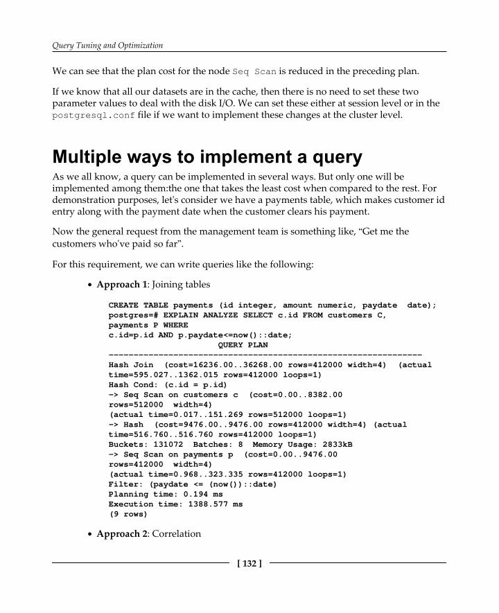
Query Tuning and Optimization

[ 132 ]

We can see that the plan cost for the node Seq Scan is reduced in the preceding plan.

If we know that all our datasets are in the cache, then there is no need to set these twoparameter values to deal with the disk I/O. We can set these either at session level or in thepostgresql.conf file if we want to implement these changes at the cluster level.

Multiple ways to implement a queryAs we all know, a query can be implemented in several ways. But only one will beimplemented among them:the one that takes the least cost when compared to the rest. Fordemonstration purposes, let's consider we have a payments table, which makes customer identry along with the payment date when the customer clears his payment.

Now the general request from the management team is something like, “Get me thecustomers who've paid so far”.

For this requirement, we can write queries like the following:

Approach 1: Joining tables

CREATE TABLE payments (id integer, amount numeric, paydate date); postgres=# EXPLAIN ANALYZE SELECT c.id FROM customers C, payments P WHERE c.id=p.id AND p.paydate<=now()::date; QUERY PLAN --------------------------------------------------------------- Hash Join (cost=16236.00..36268.00 rows=412000 width=4) (actual time=595.027..1362.015 rows=412000 loops=1) Hash Cond: (c.id = p.id) -> Seq Scan on customers c (cost=0.00..8382.00 rows=512000 width=4) (actual time=0.017..151.269 rows=512000 loops=1) -> Hash (cost=9476.00..9476.00 rows=412000 width=4) (actual time=516.760..516.760 rows=412000 loops=1) Buckets: 131072 Batches: 8 Memory Usage: 2833kB -> Seq Scan on payments p (cost=0.00..9476.00 rows=412000 width=4) (actual time=0.968..323.335 rows=412000 loops=1) Filter: (paydate <= (now())::date) Planning time: 0.194 ms Execution time: 1388.577 ms (9 rows)

Approach 2: Correlation

Query Tuning and Optimization

[ 133 ]

postgres=# EXPLAIN ANALYZE SELECT c.id FROM customers C WHERE EXISTS(SELECT 1 FROM payments P WHERE C.ID=P.ID AND p.paydate<=now()::date); QUERY PLAN -------------------------------------------------------------- Hash Semi Join (cost=16236.00..36155.50 rows=412000 width=4) (actual time=612.459..1341.980 rows=412000 loops=1) Hash Cond: (c.id = p.id) -> Seq Scan on customers c (cost=0.00..8382.00 rows=512000 width=4) (actual time=0.017..148.489 rows=512000 loops=1) -> Hash (cost=9476.00..9476.00 rows=412000 width=4) (actual time=536.628..536.628 rows=412000 loops=1) Buckets: 131072 Batches: 8 Memory Usage: 2833kB -> Seq Scan on payments p (cost=0.00..9476.00 rows=412000 width=4) (actual time=0.948..331.856 rows=412000 loops=1) Filter: (paydate <= (now())::date) Planning time: 0.232 ms Execution time: 1366.066 ms (9 rows)

Approach 3: Set operations

postgres=# EXPLAIN ANALYZE (SELECT id FROM customers C INTERSECT SELECT id FROM payments P WHERE P.paydate<=now()::date ); QUERY PLAN ----------------------------------------------------------------- SetOp Intersect (cost=131290.00..135910.00 rows=412000 width=4) (actual time=1988.390..2914.015 rows=412000 loops=1) -> Sort (cost=131290.00..133600.00 rows=924000 width=4) (actual time=1988.382..2592.499 rows=924000 loops=1) Sort Key: "*SELECT* 2".id Sort Method: external merge Disk: 16192kB -> Append (cost=0.00..27098.00 rows=924000 width=4) (actual time=3.134..861.385 rows=924000 loops=1) -> Subquery Scan on "*SELECT* 2" (cost=0.00..13596.00 rows=412000 width=4) (actual time=3.133..448.099 rows=412000 loops=1) -> Seq Scan on payments p (cost=0.00..9476.00 rows=412000 width=4) (actual time=3.129..329.192 rows=412000 loops=1) Filter: (paydate <= (now())::date) -> Subquery Scan on "*SELECT* 1" (cost=0.00..13502.00 rows=512000 width=4) (actual time=0.009..289.876 rows=512000 loops=1) -> Seq Scan on customers c (cost=0.00..8382.00 rows=512000 width=4)

Query Tuning and Optimization

[ 134 ]

(actual time=0.008..144.930 rows=512000 loops=1) Planning time: 0.153 ms Execution time: 3071.810 ms (12 rows)

If we observe the actual time from the top nodes in the preceding three approaches, all giveus the same number of rows. However, for this existing amount of data, approach 2 gave usa better performance when compared with the rest.

Approach 3 is not a good way to implement this kind of requests, since set operations likeINTERSECT have an additional sorting overhead.

So, from this preceding demonstration, we can conclude that, although we can write SQLqueries in multiple ways, we have to choose the best one, that is, the one that costs less thanthe rest.

Bad query performance with stale statisticsQuery performance always depends on the plan chosen by the Optimizer. Optimizer againdepends on the statistics of corresponding relations to generate a plan for the query. IfPostgres has stale statistics, the query might get bad plans irrespective of the existingdatasets.

For example, consider we have the following two test tables on which we perform basicoperations like the following:

CREATE TABLE out(t INTEGER);CREATE TABLE inn(t INTEGER);postgres=# SELECT COUNT(*) FROM out;count-------1000(1 row)postgres=# SELECT COUNT(*) FROM inn;count-------1000(1 row)postgres=# EXPLAIN ANALYZE SELECT * FROM out WHERE t IN(SELECT t FROMinn); QUERY PLAN----------------------------------------------------------------Hash Semi Join (cost=27.50..56.25 rows=1000 width=4) (actualtime=1.201..3.646 rows=1000 loops=1)Hash Cond: ("out".t = inn.t)

Query Tuning and Optimization

[ 135 ]

-> Seq Scan on "out" (cost=0.00..15.00 rows=1000 width=4) (actualtime=0.015..0.716 rows=1000 loops=1)-> Hash (cost=15.00..15.00 rows=1000 width=4) (actual time=1.167..1.167rows=1000 loops=1)Buckets: 1024 Batches: 1 Memory Usage: 44kB-> Seq Scan on inn (cost=0.00..15.00 rows=1000 width=4) (actualtime=0.012..0.342 rows=1000 loops=1)Planning time: 0.254 msExecution time: 3.789 ms(8 rows)

This preceding plan seems fair, and PostgreSQL has chosen the best plan based on thestatistics available. Now, for demonstration purposes, I am going to keep only one row inthe out table by deleting the rest, and then we will see the plan for the same query.

postgres=# SELECT COUNT(*) FROM out;count-------1(1 row)postgres=# EXPLAIN ANALYZE SELECT * FROM out WHERE t IN(SELECT t FROMinn); QUERY PLAN-----------------------------------------------------------------Hash Semi Join (cost=27.50..56.25 rows=1000 width=4) (actualtime=3.021..3.022 rows=1 loops=1)Hash Cond: ("out".t = inn.t)-> Seq Scan on "out" (cost=0.00..15.00 rows=1000 width=4) (actualtime=0.025..0.026 rows=1 loops=1)-> Hash (cost=15.00..15.00 rows=1000 width=4) (actual time=2.967..2.967rows=1000 loops=1)Buckets: 1024 Batches: 1 Memory Usage: 44kB-> Seq Scan on inn (cost=0.00..15.00 rows=1000 width=4) (actualtime=0.012..1.478 rows=1000 loops=1) Planning time: 0.207 ms Execution time: 3.094 ms (8 rows)

If we look at the node Seq Scan on out in this last plan, the Optimizer stillconsiders the out table to have 1000 rows in it. However, it now has only 1 row.

There can be several reasons, including the following, as to why the table statistics are notupdated:

Lazy autovacuum settingsThe stats collector process is not able to update the stats due to a huge I/O loadNo job is scheduled to run ANALYZE database manually

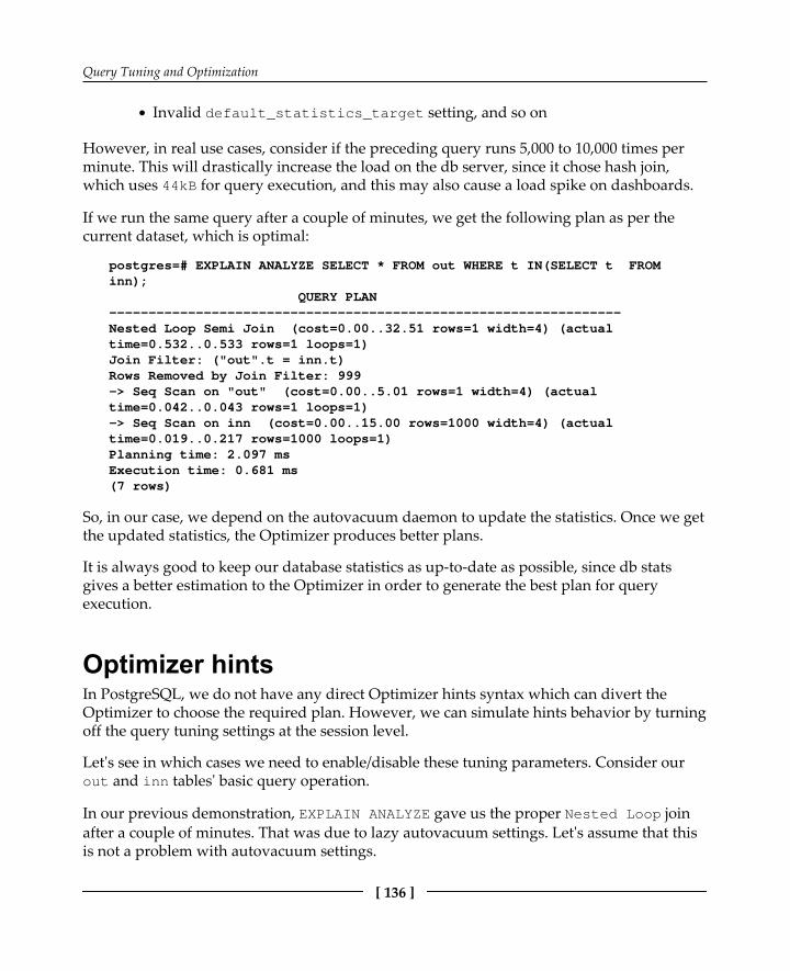
Query Tuning and Optimization

[ 136 ]

Invalid default_statistics_target setting, and so on

However, in real use cases, consider if the preceding query runs 5,000 to 10,000 times perminute. This will drastically increase the load on the db server, since it chose hash join,which uses 44kB for query execution, and this may also cause a load spike on dashboards.

If we run the same query after a couple of minutes, we get the following plan as per thecurrent dataset, which is optimal:

postgres=# EXPLAIN ANALYZE SELECT * FROM out WHERE t IN(SELECT t FROMinn); QUERY PLAN-----------------------------------------------------------------Nested Loop Semi Join (cost=0.00..32.51 rows=1 width=4) (actualtime=0.532..0.533 rows=1 loops=1)Join Filter: ("out".t = inn.t)Rows Removed by Join Filter: 999-> Seq Scan on "out" (cost=0.00..5.01 rows=1 width=4) (actualtime=0.042..0.043 rows=1 loops=1)-> Seq Scan on inn (cost=0.00..15.00 rows=1000 width=4) (actualtime=0.019..0.217 rows=1000 loops=1)Planning time: 2.097 msExecution time: 0.681 ms(7 rows)

So, in our case, we depend on the autovacuum daemon to update the statistics. Once we getthe updated statistics, the Optimizer produces better plans.

It is always good to keep our database statistics as up-to-date as possible, since db statsgives a better estimation to the Optimizer in order to generate the best plan for queryexecution.

Optimizer hintsIn PostgreSQL, we do not have any direct Optimizer hints syntax which can divert theOptimizer to choose the required plan. However, we can simulate hints behavior by turningoff the query tuning settings at the session level.

Let's see in which cases we need to enable/disable these tuning parameters. Consider ourout and inn tables' basic query operation.

In our previous demonstration, EXPLAIN ANALYZE gave us the proper Nested Loop joinafter a couple of minutes. That was due to lazy autovacuum settings. Let's assume that thisis not a problem with autovacuum settings.

Query Tuning and Optimization

[ 137 ]

If we keep on getting the same hash join plan for the single row table, then it always usesunnecessary memory for the hash buckets. To deal with this case, let's disable theenable_hashjoin Optimizer, and see the plan for the same query.

postgres=# set enable_hashjoin to off;SETpostgres=# EXPLAIN ANALYZE SELECT * FROM out WHERE t IN(SELECT t FROMinn); QUERY PLAN-----------------------------------------------------------------Merge Semi Join (cost=129.66..149.66 rows=1000 width=4) (actualtime=3.082..3.083 rows=1 loops=1)Merge Cond: ("out".t = inn.t)-> Sort (cost=64.83..67.33 rows=1000 width=4) (actual time=0.046..0.047rows=1 loops=1)Sort Key: "out".tSort Method: quicksort Memory: 25kB-> Seq Scan on "out" (cost=0.00..15.00 rows=1000 width=4) (actualtime=0.025..0.026 rows=1 loops=1)-> Sort (cost=64.83..67.33 rows=1000 width=4) (actual time=0.516..0.901rows=1000 loops=1)Sort Key: inn.tSort Method: quicksort Memory: 71kB-> Seq Scan on inn (cost=0.00..15.00 rows=1000 width=4) (actualtime=0.011..0.231 rows=1000 loops=1) Planning time: 0.185 ms Execution time: 3.171 ms (12 rows)

The preceding plan is also not an optimum one since it will merge join, which requiresadditional sort operations on both the tables. In the last plan, we see that the queryexecution uses 25kB and 71kB memory for sorting purposes.

Now, let's try to disable this Optimizer setting too, and see the plan one more time:

postgres=# set enable_mergejoin to off;SETpostgres=# EXPLAIN ANALYZE SELECT * FROM out WHERE t IN(SELECT t FROMinn); QUERY PLAN-----------------------------------------------------------------Nested Loop Semi Join (cost=0.00..15032.50 rows=1000 width=4) (actualtime=1.963..1.964 rows=1 loops=1)Join Filter: ("out".t = inn.t)Rows Removed by Join Filter: 999-> Seq Scan on "out" (cost=0.00..15.00 rows=1000 width=4) (actualtime=0.027..0.028 rows=1 loops=1)

Query Tuning and Optimization

[ 138 ]

-> Materialize (cost=0.00..20.00 rows=1000 width=4) (actualtime=0.015..1.646 rows=1000 loops=1)-> Seq Scan on inn (cost=0.00..15.00 rows=1000 width=4) (actualtime=0.012..0.660 rows=1000 loops=1)Planning time: 0.148 msExecution time: 2.058 ms(8 rows)

Yes, this last plan is what we are looking for. Once we disabled enable_hashjoin andenable_mergejoin, we got the desired and optimal plan. I am not saying that the NestedLoop join is the best of the rest. The Optimizer chooses these methods based on the volumeof the dataset which it is going to operate on. The Nested Loop method always gives thebest results on a reduced volume of data, whereas the Hash Join method gives betterresults on a moderate volume of data. The Merge Join method is best for a high volume ofdata. So, based on the volume of data, the Optimizer chooses the right method. However,the Optimizer depends on the statistics, which we need to make sure are up-to-date, to pickup the right approach to deal with the data volume.

Using the following list of Optimizer settings, we can divert the query plan:

postgres=# SELECT name FROM pg_settings WHERE name ~ 'enable_'; name-----------------enable_bitmapscanenable_hashaggenable_hashjoinenable_indexonlyscanenable_indexscanenable_materialenable_mergejoinenable_nestloopenable_seqscanenable_sortenable_tidscan(11 rows)

In some other cases, we may also need to update the column-level statistics in a table toachieve a better plan. These are the special cases where we are directly dealing with theOptimizer's source.

For demonstration, consider we have a plain table on which we perform the GROUP BYoperation:

CREATE TABLE groupbytest(t integer);postgres=# SELECT COUNT(*) FROM groupbytest;count

Query Tuning and Optimization

[ 139 ]

100000(1 row)postgres=# EXPLAIN ANALYZE SELECT COUNT(*) FROM groupbytest GROUP BY t; QUERY PLAN------------------------------------------------------------------GroupAggregate (cost=9747.82..11497.82 rows=100000 width=4) (actualtime=140.870..237.985 rows=100000 loops=1)Group Key: t-> Sort (cost=9747.82..9997.82 rows=100000 width=4) (actualtime=140.859..169.622 rows=100000 loops=1)Sort Key: tSort Method: external sort Disk: 1368kB-> Seq Scan on groupbytest (cost=0.00..1443.00 rows=100000 width=4)(actual time=0.020..19.065 rows=100000 loops=1)Planning time: 0.099 msExecution time: 253.300 ms(8 rows)

From the preceding plan, it seems the Optimizer has chosen the plan to doGroupAggregate for the GROUP BY operation. In PostgreSQL, we also haveHashAggregate, which eliminates the Sort operation required by the GroupAggregatemethod.

Now let's see the value of enable_hashagg, and let's enable it if it's not:

postgres=# SHOW enable_hashagg;enable_hashagg----------------on(1 row)

It seems enable_hashagg is ON even though the Optimizer has chosen theGroupAggregate method. To impose the HashAggregate method for the GROUP BY, wehave to understand the n_distinct column in the pg_stats table.

postgres=# SELECT n_distinct FROM pg_stats WHERE tablename = 'groupbytest'AND attname = 't';n_distinct-------------1(1 row)

We see that the value of n_distinct is -1 for the column t of the relation groupbytest.That means all the field values of an attribute t are unique values, and there are no repeatedvalues in it.

Query Tuning and Optimization

[ 140 ]

Now, let's try to impose the n_distinct value to a minimum value in the following codesnippet, and see the plan of the query:

postgres=# ALTER TABLE groupbytest ALTER COLUMN t SET(N_DISTINCT = 2);ALTER TABLE

The preceding query is saying that column t of the relation groupbytest will have onlytwo distinct values. That means all the rows in groupbytest will have repeated values.

postgres=# ANALYZE groupbytest;ANALYZEpostgres=# EXPLAIN ANALYZE SELECT COUNT(*) FROM groupbytest GROUP BY t; QUERY PLAN------------------------------------------------------------------HashAggregate (cost=1943.00..1943.02 rows=2 width=4) (actualtime=105.622..160.667 rows=100000 loops=1)Group Key: t-> Seq Scan on groupbytest (cost=0.00..1443.00 rows=100000 width=4)(actual time=0.016..19.497 rows=100000 loops=1)Planning time: 0.120 msExecution time: 174.094 ms(5 rows)

Now, if you examine the above plan for the same query, it took the HashAggregatemethod, since we diverted the Optimizer to go with a different plan as per the n_distinctsetting. If we have n_distinct value as a minimum; then the Optimizer will always try todo HashAggregate for the GROUP BY operation.

Now you might get a question like, tweaking the n_distinct setting works for the abovequery but it may not work effectively for the remaining queries. Also, it is not a goodpractice to change these settings in real production servers. To avoid the Sort operationwith GroupAggregate on column t, we have to create a sorted index, which will performan index scan on the same column rather than the sorting operation.

postgres=# CREATE INDEX sortidx ON groupbytest (t ASC);CREATE INDEXpostgres=# EXPLAIN ANALYZE SELECT COUNT(*) FROM groupbytest GROUP BY t; QUERY PLAN-----------------------------------------------------------------GroupAggregate (cost=0.29..4550.29 rows=100000 width=4) (actualtime=0.082..137.405 rows=100000 loops=1)Group Key: t-> Index Only Scan using sortidx on groupbytest (cost=0.29..3050.29rows=100000 width=4) (actual time=0.072..52.599 rows=100000 loops=1)Heap Fetches: 100000Planning time: 0.303 ms

Query Tuning and Optimization

[ 141 ]

Execution time: 148.135 ms(6 rows)

Explain PlanPostgres has a great ability to show you how it will actually execute a query under thecovers. This is known as an execution plan, and it is exposed by the explain command.Understanding this tells you how you can optimize your database with indexes to improveperformance.

Every query within Postgres has an execution plan when executed. There are three ways torun explain to expose this to you:

The generic form (only shows what is likely to happen)The Analyze form (which actually runs the query, and outputs what doeshappen)The Verbose form (verbose information)

Most commonly, explain is run on the SELECT statements. However, you can also use it onthe following:

INSERT

UPDATE

DELETE

EXECUTE

DECLARE

Generating and reading the Explain PlanFor each step in the execution plan, EXPLAIN prints the following information:

The type of operation required.The estimated cost of execution.If you specified EXPLAIN ANALYZE, it gives the actual cost of execution. If youomit the ANALYZE keyword, the query is planned but not executed, and the actualcost is not displayed.

Query Tuning and Optimization

[ 142 ]

Simple exampleLet's start by looking at a simple example:

perf=# EXPLAIN ANALYZE SELECT * FROM recalls; QUERY PLAN:Seq Scan on recalls (cost=0.00..9217.41 rows=39241 width=1917)(actualtime=69.35..3052.72 rows=39241 loops=1)Total runtime: 3144.61 msec

In this preceding example, PostgreSQL has decided to perform a sequential scan of therecalls table (Seq Scan on recalls). There are three data items in the cost estimate:

The first set of numbers (cost=0.00..9217.41) is an estimate of how expensivethis operation will be. Expensive is measured in terms of disk reads. Twonumbers are given:

The first number represents how quickly the first row in the resultset can be returned by the operation.The second (which is usually the most important) represents howlong the entire operation should take. The second data item in thecost estimate (rows=39241) shows how many rows PostgreSQLexpects to return from this operation.

The final data item (width=1917) is an estimate of the width, in bytes, of theaverage row in the result set.If you include the ANALYZE keyword in the EXPLAIN command, PostgreSQL willexecute the query, and display the actual execution costs. This was a simpleexample. PostgreSQL required only one step to execute this query (a sequentialscan on the entire table). Many queries require multiple steps, and the EXPLAINcommand will show you each of those steps.

More complex exampleLet's now move on to a more complex example:

perf=# EXPLAIN ANALYZE SELECT * FROM recalls ORDER BY yeartxt;NOTICE: QUERY PLAN:Sort (cost=145321.51..145321.51 rows=39241 width=1911)(actual time=13014.92..13663.86 rows=39241 loops=1)-> Seq Scan on recalls (cost=0.00..9217.41 rows=39241 width=1917) (actualtime=68.99..3446.74 rows=39241 loops=1)Total runtime: 16052.53 msec

Query Tuning and Optimization

[ 143 ]

This last example shows a two-step query plan. In this case, the first step is actually listed atthe end of the plan. When you read a query plan, it is important to remember that each stepin the plan produces an intermediate result set. Each intermediate result set is fed into thenext step of the plan.

Looking at this plan, PostgreSQL first produces an intermediate result set byperforming a sequential scan (Seq Scan) on the entire recalls table. That stepshould take about 9,217 disk page reads, and the result set will have about 39,241rows, averaging 1,917 bytes each. Notice that these estimates are identical tothose produced in the first example. And in both cases, you are executing asequential scan on the entire table.After the sequential scan has finished building its intermediate result set, it is fedinto the next step in the plan. The final step in this particular plan is a sortoperation, which is required to satisfy our ORDER BY clause. The sort operationreorders the result set produced by the sequential scan, and returns the finalresult set to the client application.An ORDER BY clause does not require a sort operation in all cases. ThePlanner/Optimizer may decide that it can use an index to order the result set.

Query operatorsPostgreSQL currently has 19 query operators.

Seq ScanThe Seq Scan operator is the most basic query operator. Any single-table query can becarried out using the Seq Scan operator.

Index ScanAn Index Scan operator works by traversing an index structure. If you specify a startingvalue for an indexed column (WHERE record_id >= 1000, for example), the Index Scanwill begin at the appropriate value. If you specify an ending value (such as WHERErecord_id < 2000), the Index Scan will complete as soon as it finds an index entrygreater than the ending value.

Query Tuning and Optimization

[ 144 ]

SortThe Sort operator imposes an ordering on the result set. PostgreSQL uses two different sortstrategies: an in-memory sort and an on-disk sort. You can tune a PostgreSQL instance byadjusting the value of the work_mem runtime parameter.

UniqueThe UNIQUE operator eliminates duplicate values from the input set. The input set must beordered by the columns, and the columns must be unique.

LIMITThe LIMIT operator is used to limit the size of a result set.

AggregateThe Planner/Optimizer produces an AGGREGATE operator whenever the query includes anaggregate function. The following functions are aggregate functions: AVG(), COUNT(),MAX(), MIN(), STDDEV(), SUM(), and VARIANCE().

AppendThe Append operator is used to implement a UNION. An Append operator will have two ormore input sets.

ResultThe Result operator is used to execute a query that does not retrieve data from a table, forexample, executing functions.

Query Tuning and Optimization

[ 145 ]

Nested LoopThe Nested Loop operator is used to perform a join between two tables. A Nested Loopoperator requires two input sets (given that a Nested Loop joins two tables, this makesperfect sense).

Merge JoinThe Merge Join operator also joins two tables. Like the Nested Loop operator, MergeJoin requires two input sets: an outer table and an inner table. Each input set must beordered by the join columns.

Hash and Hash JoinThe Hash and Hash Join operators work together. The Hash Join operator requires twoinput sets, again called the outer and inner tables.

GroupThe Group operator is used to satisfy a GROUP BY clause. A single input set is required bythe Group operator, and it must be ordered by the grouping column(s).

Subquery Scan and SubplanA Subquery Scan operator is used to satisfy a UNION clause; Subplan is used forsubselects. These operators scan through their input sets, adding each row to the result set.

Tid ScanThe Tid Scan (tuple ID scan) operator is rarely used. A tuple is roughly equivalent to arow. Every tuple has an identifier that is unique within a table; this is called the tuple ID.

Query Tuning and Optimization

[ 146 ]

MaterializeThe Materialize operator is used for some subselect operations. The Planner/Optimizermay decide that it is less expensive to materialize a subselect once than to repeat the workfor each top-level row.

SetopThere are four Setop operators: Setop Intersect, Setop Intersect All, SetopExcept, and Setop Except All. These operators are produced only when thePlanner/Optimizer encounters an INTERSECT, INTERSECT ALL, EXCEPT, or EXCEPT ALLclause, respectively.

SummaryThis chapter started with tuning queries and continued with how caching benefits theexecution of a query. So simply writing a query and expecting a good performance is notalways enough. There are multiple ways to tune queries for better performance, which wecovered them in this chapter, to help you write queries. We also covered how to tweak theconfiguration settings to get the best performance from disks, and how to use Optimizerhints to let it choose the best plan. We discussed generating and reading Explain Plan, andeach node in the Explain Plan. In the next chapter, we will cover in-built extensions inPostgreSQL, how to build contrib modules, and dblinks. These days many applicationsneed images to be stored in their database as part of their operations, so we will also coverlarge objects in the next chapter.

9PostgreSQL Extensions and

Large Object SupportIn the previous chapter, we talked about the process of query execution and found out whatwent wrong by looking at plans, then fixing it. Sometimes, a query itself could be the reasonfor performance issues, so we talked about tuning as well; and sometimes, it is just thatsome settings need to be changed to make a query perform better. We also coveredavailable caches and how to install them as extensions. In this chapter, we will coverextensions.

What is an extension?How do we create/build/install them?How do we use database links?Importing/exporting images into databases

Creating an extensionExtensions are one of the nice features in PostgreSQL. These were introduced inPostgreSQL 9.1. An extension is simply a bunch of SQL together in a script file. So, creatingan extension loads the objects into the database. For example, a new datatype will requirenew functions, new operators, and probably new index operator classes. It is helpful tocollect all these objects in a single package to simplify database management. PostgreSQLcalls such a package an extension.

PostgreSQL Extensions and Large Object Support

[ 148 ]

The following is the syntax to create an extension:

CREATE EXTENSION [ IF NOT EXISTS ] extension_name[ WITH ] [ SCHEMA schema_name ] [ VERSION version ] [ FROM old_version ]

Let's take an example of creating a simple extension, pg_stat_statements, and the objectsloaded by creating it:

postgres=# CREATE EXTENSION pg_stat_statements ;CREATE EXTENSION

The functions created are as follows:

postgres=# \df pg_stat_statement*List of functions-[ RECORD 1 ]--------+------ Schema | public Name | pg_stat_statements Result data type | SETOF record Argument data types | showtext boolean, OUT userid oid, OUT dbid oid, OUT queryid bigint, OUT query text, OUT calls bigint, OUT total_time double precision, OUT min_time double precision, OUT max_time double precision, OUT mean_time double precision, OUT stddev_time double precision, OUT rows bigint, OUT shared_blks_hit bigint, OUT shared_blks_read bigint, OUT shared_blks_dirtied bigint, OUT shared_blks_written bigint, OUT local_blks_hit bigint, OUT local_blks_read bigint, OUT local_blks_dirtied bigint, OUT local_blks_written bigint, OUT temp_blks_read bigint, OUT temp_blks_written bigint, OUT blk_read_time double precision, OUT blk_write_time double precision Type | normal-[ RECORD 2 ]-----------+ Schema | public Name | pg_stat_statements_reset Result data type | void Argument data types | Type | normalView created:postgres=# \dv pg_stat_statement*List of relations-[ RECORD 1 ]-------------- Schema | public Name | pg_stat_statements Type | view Owner | postgres

PostgreSQL Extensions and Large Object Support

[ 149 ]

We can see that an extension is created in a public schema. So, if we do not provide anyschema as an owner while creating an extension, it creates an extension in the schema,which is in search_path. If we want the extension in a particular schema, then the syntaxis as follows:

postgres=# DROP EXTENSION IF EXISTS pg_stat_statements;DROP EXTENSIONpostgres=# CREATE EXTENSION pg_stat_statements WITH SCHEMA ext_owner;CREATE EXTENSION

If you want to change the schema of an extension, you can alter the schema once it iscreated. You can use the following syntax:

postgres=# ALTER EXTENSION pg_stat_statements SET SCHEMA public;ALTER EXTENSION

Compiling extensionsWe talked about creating extensions in the preceding topic; however, we can only createextensions that are already compiled against our installation. We can see availableextensions in the pg_available_extensions catalog.

postgres=# SELECT * FROM pg_available_extensions limit 1;-[ RECORD 1 ]-----+---------------------------------------name | adminpackdefault_version | 1.0installed_version | 1.0comment | administrative functions for PostgreSQL

We cannot create an extension that is not already compiled, for example:

postgres=# SELECT * FROM pg_available_extensions WHERE name='postgis';name | default_version | installed_version | comment-----+-----------------+-------------------+---------(0 rows)postgres=# create extension postgis;ERROR: could not open extension control file"/Library/PostgreSQL/9.4/share/postgresql/extension/postgis.contro l": Nosuch file or directorypostgres=#

If you observe, postgis is not available in the list, so we could not create extension. So,how do we deal with such kinds of extension? For this, we will compile the source withPostgreSQL installation. Let's compile and create a postgis extension.

PostgreSQL Extensions and Large Object Support

[ 150 ]

Here are the higher-level steps to install PostGIS on a Linux machine:

Download the PostGIS source from h t t p : / / p o s t g i s . n e t / s o u r c e /

Untar the file and configure it using your current pg_config path:

./configure --with-pgconfig=/path/to/your/pg_config

Execute make and make install to create libraries and install binaries

However, you can find detailed installation for various platforms on h t t p : / / t r a c . o s g e o . o

r g / p o s t g i s / w i k i / U s e r s W i k i I n s t a l l.

Now, let's check if you have PostGIS in the available extensions list:

postgres=# SELECT * FROM pg_available_extensions WHERE name='postgis';-[ RECORD 1 ]-----+----------------------------------------name |postgisdefault_version | 2.2.2installed_version |comment | PostGIS geometry, geography, and raster spatial types and functions(1 row)

Now, if you try to create a PostGIS extension:

postgres=# CREATE EXTENSION postgis;CREATE EXTENSIONpostgres=#

In this way, we can build extensions from the source code, even though they are not in theextensions list available with the default installation.

Database links in PostgreSQLLet's see a use case to explain why we will need database links at all. Let's say you wantoutput from a table, function, or any other object of a database that is different to the oneyou are connected to. Then, generally, you will connect to the other database and fetch thedata. However, if you are doing this through a function, then it will not be possible for youto connect to other databases within the function. However, using db links, you do not needto connect to that database; instead, you just access those databases using db links.

PostgreSQL Extensions and Large Object Support

[ 151 ]

Unlike some of the other popular RDBMS databases, PostgreSQL does not have a CREATEDATABASE command. However, there are a few functions to access objects of differentdatabases. You will need to create a dblink extension to get those functions. The syntax isas follows:

postgres=# CREATE SCHEMA for_dblink;CREATE SCHEMApostgres=# CREATE EXTENSION dblink WITH SCHEMA for_dblink;CREATE EXTENSION

You will see the dblink functions using the following command:

postgres=# \df for_dblink.dblink*List of functionsSchema | Name | Result data type | Argument data types | Type-------+------+------------------+---------------------+------for_dblink | dblink | SETOF record | text | normalfor_dblink | dblink | SETOF record | text, boolean | normalfor_dblink | dblink | SETOF record | text, text | normalfor_dblink | dblink | SETOF record | text, text, boolean | normal...

Here is an example of how to use the preceding links.

PostgreSQL Extensions and Large Object Support

[ 152 ]

Let's establish a connection to the database before you use them:

postgres=# SELECT dblink_connect('test_conn','dbname=postgres');dblink_connect----------------OK(1 row)

In the preceding example, test_conn is the connection name that you can use later in thesame session, and dbname is the name of the db you want to connect with in order to execute the queries.

To execute a query, we will use the following syntax:

postgres=# SELECT * FROM dblink('test_conn','select ''testing_db_conn''')as test(string varchar);string-----------------testing_db_conn(1 row)

We will use the same connection, test_conn, to execute a query so it connects to thepostgres database to run the query. You must specify the return datatype of the callingquery to display values.

So SELECT works fine. How about DDL and DMLs? Let's try these:

postgres=# SELECT * FROM dblink('test_conn','create table dblink_test(idint)') as test(result varchar);result--------------CREATE TABLE(1 row)postgres=# SELECT * FROM dblink('test_conn','select * from dblink_test')as test(result varchar);result--------(0 rows)

The same function can be used for DDLs as well. Now, let's test DMLs:

postgres=# SELECT * FROM dblink('test_conn','insert into dblink_testvalues(1)') as test(result varchar);result------------INSERT 0 1(1 row)postgres=# SELECT * FROM dblink('test_conn','select * from dblink_test')

PostgreSQL Extensions and Large Object Support

[ 153 ]

as test(result varchar);result--------1(1 row)postgres=# SELECT * FROM dblink('test_conn','update dblink_test set id=2where id=1') as test(string varchar);string----------UPDATE 1(1 row)postgres=# SELECT * FROM dblink('test_conn','select * from dblink_test')as test(result varchar);result--------2(1 row)postgres=# SELECT * FROM dblink('test_conn','delete from dblink_test') astest(string varchar);string----------DELETE 1(1 row)postgres=# SELECT * FROM dblink('test_conn','select * from dblink_test')as test(result varchar);result--------(0 rows)

As per the preceding tests, the dblink function can be used for SELECT, DDLs, and DMLs.

You can check out the usage of other dblink functions on h t t p : / / w w w . p o s t g r e s q l . o r g / d

o c s / 9 . 5 / s t a t i c / d b l i n k . h t m l.

Using binary large objectsWhat if someone wants to store a picture, Word document, or PDF, in a database? For this,PostgreSQL has a large object facility that provides stream-style access to user data, whichis stored in a special large-object structure. Streaming access is useful when you areworking with data values that are too large to manipulate conveniently as a whole.

The large object implementation breaks large objects into chunks and stores them in rows inthe database. A B-tree index guarantees fast searches for the correct chunk number whendoing random-access reads and writes.

PostgreSQL Extensions and Large Object Support

[ 154 ]

How do we implement it? As this book is intended to teach you the basics, let's look at howto create/implement large objects:

Creating a large objectYou can use the lo_creat function to create a large object. The syntax is as follows:

Oid lo_creat(PGconn *conn, int mode);

The return value is Oid.

Here's an example:

inv_oid = lo_creat(conn, INV_READ|INV_WRITE);

The Oid lo_create(PGconn *conn, Oid lobjId); function also creates a new largeobject. The OID to be assigned can be specified by lobjId; if so, failure occurs if that OIDis already in use for some large object. If lobjId is InvalidOid (zero) then lo_createassigns an unused OID (this is the same behavior as lo_creat). The return value is OIDthat was assigned to the new large object, or InvalidOid (zero) on failure.

The lo_create is new as of PostgreSQL 8.1; if this function is run against an older serverversion, it will fail and return InvalidOid.

Here's an example:

inv_oid = lo_create(conn, desired_oid);

Importing a large objectYou can use the lo_import function to import the large object into the database:

Oid lo_import(PGconn *conn, const char *filename);

The filename attribute specifies the operating system name of the file to be imported as alarge object. The return value is an OID.

PostgreSQL Extensions and Large Object Support

[ 155 ]

Exporting a large objectTo export a large object into an operating system file, use the lo_export as shown:

int lo_export(PGconn *conn, Oid lobjId, const char *filename);

The lobjId argument specifies an OID of the large object to export, and the filenameargument specifies the operating system name of the file. Note that the file is written by theclient interface library not the server. It returns 1 on success, -1 on failure.

Writing data to a large objectTo write data to a large object, you can use the lo_write function, as shown:

int lo_write(PGconn *conn, int fd, const char *buf, size_t len);

This writes len bytes from buf (which must be of size len) to the large object descriptor fd.The fd argument should be returned by a previous lo_open. The number of bytes actuallywritten is returned (in the current implementation, this will always equal len unless thereis an error). In the event of an error, the return value is -1.

Although the len parameter is declared as size_t, this function will reject length valueslarger than INT_MAX. In practice, it's best to transfer data in chunks of a few megabytes atthe most.

We have taken examples from the PostgreSQL documentation; these are simple and clear.You can check out h t t p : / / w w w . p o s t g r e s q l . o r g / d o c s / c u r r e n t / s t a t i c / l o - i n t e r f a c e s . h

t m l # L O - C R E A T E to learn how to read/seek/close large objects.

Here is an example function with which you can test: h t t p : / / w w w . p o s t g r e s q l . o r g / d o c s / c

u r r e n t / s t a t i c / l o - e x a m p l e s e c t . h t m l.

Server-side functionsPostgreSQL also has server-side functions that you can execute in database. You canconnect to the database and, using SQLs, insert and fetch large objects. Let's look at anexample:

postgres=# CREATE TABLE image_load(name text, image oid);CREATE TABLEpostgres=#postgres=# INSERT INTO image_load VALUES('my_image',

PostgreSQL Extensions and Large Object Support

[ 156 ]

lo_import('/tmp/pic.png'));INSERT 0 1postgres=#

You can specify an OID while importing:

postgres=# INSERT INTO image_load VALUES('my_image',lo_import('/tmp/pic.png',123456));INSERT 0 1

And export it using the following query:

postgres=# select lo_export(image_load.image, '/tmp/pic.png') fromimage_load ;lo_export----------1(1 row)

SummaryIn this chapter, we covered how to create, compile, and install extensions. Every extensionhas its own usage, so simply creating extensions that you do not use does not hurt much;however, it unnecessarily increases the count of objects in the database. As PostgreSQL isthe most popular open source database, there are plenty of contrib and external extensionsthat are available in the market openly. Additionally, we also covered db links, which isuseful when you are working with multiple databases. There are many applications thatstore large objects in the database, so we took a look at those as well. In the next chapter, wewill cover how to connect Postgre with PHP, and how to deal with DDLs, DMLs, andSELECT with PHP. We will describe this with practical examples that will help you testyourself locally before implementing your actual requirements.

10Using PHP in PostgreSQL

In the previous chapter, we covered what an extension is and how it's useful. We alsocovered how to create an extension and compile an extension that is not available bydefault. Additionally, we also talked about the dblink extension and how it is useful in thereal world. The examples that we described gave you a better understanding of how thosework and how to use them. In this chapter, we will work on PHP with Postgres. We startwith a simple connection to Postgres with PHP and then talk about how to use DDLs,DMLs, and fetching data. We will talk about the available functions of PHP when workingwith SQLs.

Postgres with PHPIn this chapter, we will discuss how to use PostgreSQL with web services such asApache/PHP, which is one of the most famous web services available in the market. In thischapter, we will demonstrate all the concepts using

Apache/2.4.7 (Ubuntu)PHP Version => 5.5.9-1ubuntu4.16PostgreSQL(libpq) Version => 9.3.11

As the scope of the book is limited to Postgres development essentials, we hope that youhave basic apache/PHP skills, which is the reason we are directly jumping into the PHPscripting sections.

Using PHP in PostgreSQL

[ 158 ]

PHP-to-PostgreSQL connectionsTo make a connection to PostgreSQL from PHP, we have a set of built-in functions wherewe need to pass our connection string and a set of client options to make a connection.Here, we have the pg_connect() and pg_pconnect() functions in PHP that will get theconnection from PostgreSQL.

Now, let's try a simple connection to Postgres using PHP:

<?php$dbcon = pg_connect("host=localhost port=5432 dbname=postgresuser=postgres");

if (!$dbcon) { echo"Unable to make connection"; exit;}else { echo"Successfully made connection to PostgreSQL\n";}?>

To run the PHP code, we need to either embed the code in an HTML file and then call theweb page or we can use the PHP command-line interface.

The result is as follows:

$ php /tmp/test.phpSuccessfully made connection to PostgreSQL

In the preceding code, we used the pg_connect function to make a connection to thedatabase. If this function is able to make the connection successfully, then it returns a non-empty resource and an empty resource if it fails to connect to the database.

And we also have another function, pg_pconnect(), which makes a persistent connectionto PostgreSQL. Persistent connections are useful to reuse existing connections if any newconnection is needed. One real use case for persistent connection is that, using thepg_pconnect() method, we can use the same database connection during multiple pagereloads. There are also some caveats about persistent connections that we need to take careof. You can refer to the pros and cons of persistent connections at h t t p : / / p h p . n e t / m a n u a l /

e n / f e a t u r e s . p e r s i s t e n t - c o n n e c t i o n s . p h p.

Using PHP in PostgreSQL

[ 159 ]

To demonstrate a persistent connection, let's try to get the same database connection twice,as shown next.

Let's create a PHP file with the getDBConnection() function, which we have called in theprevious chapters:

$ catpgconnection.php<?php

functiongetPDBConnection() { $dbcon = pg_pconnect("host=localhostdbname=postgres user=postgres");

if (!$dbcon) { echo"Unable to make connection\n"; exit; } else { echo"Successfully made persistent connection to PostgreSQL\n"; echo"pg connection pid is "; echo pg_get_pid($dbcon); echo"\n"; return $dbcon; } }

functiongetDBConnection() { $dbcon = pg_connect("host=localhostdbname=postgres user=postgres"); if (!$dbcon) { echo"Unable to make connection\n"; exit; } else { echo"Successfully made connection to PostgreSQL\n"; echo"pg connection pid is "; echo pg_get_pid($dbcon); echo"\n"; return $dbcon; }}?>

Now, let's write the test.php file including the preceding PHP file, as shown in thefollowing code:

$ cattest.php<?phpinclude'pgconnection.php';$con=getPDBConnection();

Using PHP in PostgreSQL

[ 160 ]

pg_close($con);$con=getPDBConnection();pg_close($con);?>

If you see the preceding code, we close the database connection using pg_close once wehave got the database connection.

$ phptest.phpSuccessfully made persistent connection to PostgreSQLpg connection pid is 91258Successfully made persistent connection to PostgreSQLpg connection pid is 91258

From the previous result, we got the same Postgres connection, the pid is 91258, eventhough we closed the connection using pg_close. Now, let's try the same code withpg_connect() and see the impact:

<?phpinclude'pgconnection.php';

$con=getDBConnection();pg_close($con);$con=getDBConnection();pg_close($con);?>$ phptest.phpSuccessfully made persistent connection to PostgreSQLpg connection pid is 91271Successfully made persistent connection to PostgreSQLpg connection pid is 91272

The moment we changed the behavior of getting a connection from pg_pconnect() topg_connect(), we got two different connection pids for each function call. This is due tothe pg_close() function that is not effective against persistent connections. If we changethe connection string to pg_pconnect(), we will get a new persistent connection.

We can create an asynchronous connection to Postgres using PGSQL_CONNECT_ASYNC as anoption for the pg_connect()/pg_pconnect() functions, and use the pg_connect_poll(resource) function to check connection availability. However, these functionalities havebeen added from the PHP 5.6.0 version onwards.

Using PHP in PostgreSQL

[ 161 ]

Dealing with DDLsIn PHP, we have the pg_query() function that we use to execute all kinds of SQLstatement. We can use this function to execute either DDL or DML statements. This functiontakes two arguments; one is the db connection resource and the other is an SQL statement.To track the SQL statement status, we have the pg_last_error() function, which takesthe db connection as its argument.

Now, let's try to create a test table using the preceding getDBConnection()

<?phpinclude'pgconnection.php';

$con=getDBConnection();$sql =<<<EOFCREATE TABLE test(d char(1));EOF;

if (pg_query($con, $sql)) { echo"test table is created successfully\n";}else{ echo"Failed in creating table\n"; echopg_last_error($con); echo"\n";}?>

$ phptest.phpSuccessfully made connection to PostgreSQLpg connection pid is 91659test table is created successfully

Let's run the same PHP script and see what error we get:

$ phptest.phpSuccessfully made connection to PostgreSQLpg connection pid is 5369PHP Warning: pg_query(): Query failed: ERROR: relation "test" alreadyexists in /tmp/test.php on line 24Failed in creating tableERROR: relation "test" already exists

As expected, we got an ERROR saying that the relation already exists.

Using PHP in PostgreSQL

[ 162 ]

In PHP, we can also use pg_execute() to execute any DML or DDL statements. All SQLstatements that we execute will get fired on the database as a single statement as an implicittransaction. We can also run the set of SQL statements explicitly as shown in the followingcode:

$sql =<<<EOFCREATE TABLE test(d char(1));ALTER TABLE test ADD column d2 char(1);EOF;

Otherwise, we can also initiate one pg_query() to begin the transaction, and onepg_query() to close the transaction as shown in the following code

pg_query($con, "BEGIN");

$sql =<<<EOFCREATE TABLE test(column1 char(1));ALTER TABLE test ADD column column2 char(1);EOF;if (pg_query($con, $sql)) { echo"test table is created successfully\n"; pg_query($con, "END");}else { echo"Failed in creating table\n"; echopg_last_error($con); echo"\n";}

DML operationsTo execute a DML operation against the database, we can use a set of pg_* functions. Wecan use the same functions for all DML operations.

pg_query/pg_query_params/pg_insert/pg_update/pg_delete

First, let's try to insert records into the database with pg_query:

$sql=<<<EOFINSERT INTO test VALUES('A', 'B');INSERT INTO test VALUES('I', 'U');EOF;

if (pg_query($con, $sql)) { echopg_affected_rows($con); echo " Records are inserted

Using PHP in PostgreSQL

[ 163 ]

successfully";}else { echo"Failed inserting records"; echopg_last_error($con); echo"\n";}

Result:

$ php /tmp/test.phpSuccessfully made connection to PostgreSQLpg connection pid is 921532 Records are inserted successfully

If we want to know how many records our code inserted, then we will have to usepg_affected_rows($con) after executing the INSERT statements.

pg_query_paramsUsing the pg_query_params function, we can pass a set of arguments to the SQL query.This is the benefit of using this function over pg_query, where we can pass arguments tothe actual SQL. Additionally, the pg_query_params function accepts only one DML SQLquery, unlike the pg_query function. Another benefit we get from pg_query_params() isthat it gives protection against SQL injections. Refer to h t t p : / / p h p . n e t / m a n u a l / e n / f u n c t i

o n . p g - q u e r y - p a r a m s . p h p, for more details on preventing SQL injections.

if(pg_query_params($con, 'INSERT INTO dummy VALUES($1, $2)', array("I","U"))) { echopg_affected_rows($con); echo" Records are inserted successfully";}else { // Exception section here ....}

In the preceding code snippet, we have used $1 and $2 to represent the field values asarguments and array("I", "U") to represent the argument values. Here, $1="I" and$2="U". In pg_query_params(), $1, $2, and ..$n always map to array (value-1, value-2, …value-n).

Using PHP in PostgreSQL

[ 164 ]

pg_insertThe pg_insert function gives a more programmatical approach to inserting records into atable. This function takes three arguments. First one is the database connection name,second one is table name, and the last one is column name associated with table. Anassociate array should be "fieldname"=>"value".

For example, let's use the same example we used for pg_query_params with pg_insert,as shown in the following code:

if (pg_insert($con, 'test', array("column1"=>"A", "column2"=>"B"))) { echopg_affected_rows($con); echo " Records are inserted successfully";}else { echo"Failed inserting records"; echopg_last_error($con);}

Using the pg_query(), pg_query_params(), or pg_insert() functions, we can executeDML operations. All the approaches we see, submit the query to the database engine, andthe database will parse it and generate a plan. Each time you call these functions, the dbengine needs to perform these parsing and generating plans. If you execute the precedingfunctions in any of the loops it will become a performance issue.

To avoid this, we will use pg_execute() along with the pg_prepare() function. Thepg_prepare() function takes three arguments, namely, connection resource, statementname, and parameterized SQL query. Here, the prepared statement name can be anything.It does not have to be related to any object name in the database. The syntax is as follows:

pg_prepare($con, "loopStmt", "INSERT INTO test VALUES($1, $2)")

Once the pg_prepare() execution is successful, we will get "loopStmt" as the preparedstatement name, which we will use in all the pg_execute() function calls.

Here is a sample implementation:

if (pg_prepare($con, 'loopStmt', 'INSERT INTO test VALUES($1, $2)')) { echo"Prepared statement is created\n";

if (pg_execute($con, 'loopStmt', array("i", "u"))) { echo"Executed prepared statement successfully\n"; }}

Using PHP in PostgreSQL

[ 165 ]

Result:

$ php /tmp/test.phpSuccessfully made connection to PostgreSQLpg connection pid is 93104Prepared statement is createdExecuted prepared statement successfully

Data retrievalTo retrieve records from the database, we can use the same functions that we used toINSERT records into a database, except pg_insert(). To retrieve the records or to navigatetuples one by one, we need to use some other functions where we can traverse the completequery result set.

Now let's discuss query retrieval functions one by one.

pg_fetch_allOnce we execute our SQL query using pg_execute, pg_query, or pg_query_params, wecan use pg_fetch_all; this takes the data resource as an argument and returns an array,which holds our complete query result set.

The following is an example:

<?php...$con=getDBConnection();

$res=pg_query($con, "SELECT * FROM test");$arr=pg_fetch_all($res);

echo"Complete result set\n";print_r($arr);?>

In the preceding PHP code, we used $res as an argument for pg_fetch_all(). which is apointer to the query result set.

Result:

$ php /tmp/test.phpSuccessfully made connection to PostgreSQL

Using PHP in PostgreSQL

[ 166 ]

pg connection pid is 93342Complete result setArray([0] => Array([column1] => A[column2] => B)

[1] => Array([column1] => I[column2] => U))

pg_fetch_assocThe pg_fetch_assoc function is similar to pg_fetch_all, but pg_fetch_assoc gives amuch more convenient way to play with the result set. That is, using pg_fetch_all(), wewill not have control over the order of columns as they appear in the SELECT statement inthe result set. If we made any SQL query changes, pg_fetch_all() gives a different arraywith brand-new column indexes. The pg_fetch_assoc() function also takes the result setas an input and returns an associate array where the column names are keys that will giveus more flexiblility while traversing the result set.

<?phpinclude'pgconnection.php';

$con=getDBConnection();

$res = pg_query($con, "SELECT * FROM test");if (!$res) { echo"An error occurred.\n"; exit;}while ($row = pg_fetch_assoc($res)) { echo $row['column1']; echo "\t"; echo $row['column2']; echo "\n";}?>

$ php /tmp/test.phpSuccessfully made connection to PostgreSQL

Using PHP in PostgreSQL

[ 167 ]

pg connection pid is 93518a bi u

From the preceding example, $row is an assoc array, and we used a column name as a keyto get the actual record values.

pg_fetch_resultUsing the pg_fetch_result function, we can fetch the required specific data value fromthe result set. This function takes three arguments: the result set, row number, and therequired field number, as shown in the following example:

<?phpinclude'pgconnection.php';

$con=getDBConnection();

$res = pg_query($con, "SELECT * FROM test");if (!$res) { echo"An error occurred.\n"; exit;}

$val=pg_fetch_result($res, 0, 0);echo"Row(0,0) $val\n";$val=pg_fetch_result($res, 0, 1);echo"Row(0,1) $val\n";?>

Result:

$ php /tmp/test.phpSuccessfully made connection to PostgreSQLpg connection pid is 7221Row(0,0) aRow(0,1) b

Using PHP in PostgreSQL

[ 168 ]

Helper functions to deal with data fetchingThere are other helper functions that help you retrieve the results. Let's go through thesefunctions one by one:

pg_free_resultsUsing the pg_free_results function, we can clear the memory resources that are used tohold the result set. All the data retrieval functions we used earlier occupy a certain amountof memory to hold the result set. It is a good practice to clear the result set after we are doneprocessing the query results.

pg_num_rowsUsing the pg_num_rows function, we can get the number of tuples in the result set. That is,if we execute a query, it returns the number of tuples the SELECT query has fetched fromthe database.

pg_num_fieldsUsing the pg_num_fields function, we can get the number of columns or fields in theresult set. That is, it returns the number of columns we mentioned in the SELECT query.

pg_field_nameUsing pg_field_name function, we can get the field name that we mentioned in theSELECT query. This function takes the result source as the first argument and the columnposition in the mentioned SELECT query as a second argument, which will return thecolumn name associated with that numeric field.

pg_meta_dataUsing the pg_meta_data function, we can get the meta information about the table. That is,we can get the complete table definition in an array format.

Using PHP in PostgreSQL

[ 169 ]

pg_convertUsing the pg_convert function, we can convert the associate array to proper SQLconverted values by comparing the actual table definition.

The following is an example:

<?phpinclude'pgconnection.php';

$con=getDBConnection();

$res = pg_query($con, "SELECT * FROM test");if (!$res) { echo"An error occurred.\n"; exit;}

echo"Table defintion\n";$meta = pg_meta_data($con, 'test');var_dump($meta);

$val = pg_num_rows($res);echo"Number of records: $val\n";

$val = pg_num_fields($res);echo"Number of fields: $val\n";

$col1 = pg_field_name($res, 0);echo"Column 1 is: $col1\n";

$col2 = pg_field_name($res, 1);echo"Column 2 is: $col2\n";

$vals = array( 'column1' =>'u', 'column2' =>'i');

$stmt_helper = pg_convert($con, 'dummy', $vals);echo"pg_convert array is:\n";print_r($stmt_helper);?>

Using PHP in PostgreSQL

[ 170 ]

Result:

Successfully made connection to PostgreSQLpg connection pid is 7350Table defintionarray(2) { ["column1"]=>array(6) { ["num"]=>int(1) ["type"]=>string(6) "bpchar" ["len"]=>int(-1) ["not null"]=>bool(false) ["has default"]=>bool(false) ["array dims"]=>int(0) } ["column2"]=>array(6) { ["num"]=>int(2) ["type"]=>string(6) "bpchar" ["len"]=>int(-1) ["not null"]=>bool(false) ["has default"]=>bool(false) ["array dims"]=>int(0) }}Number of records: 4Number of fields: 2Column 1 is: column1Column 2 is: column2pg_convert array is:Array(["column1"] => E'U'["column2"] => E'I')

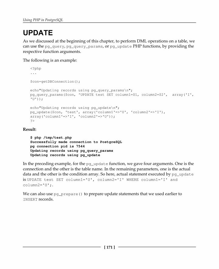
Using PHP in PostgreSQL

[ 171 ]

UPDATEAs we discussed at the beginning of this chapter, to perform DML operations on a table, we can use the pg_query, pg_query_params, or pg_update PHP functions, by providing therespective function arguments.

The following is an example:

<?php...

$con=getDBConnection();

echo"Updating records using pg_query_params\n";pg_query_params($con, 'UPDATE test SET column1=$1, column2=$2', array('I','U'));

echo"Updating records using pg_update\n";pg_update($con, 'test', array('column1'=>'U', 'column2'=>'I'),array('column1'=>'I', 'column2'=>'U'));?>

Result:

$ php /tmp/test.phpSuccessfully made connection to PostgreSQLpg connection pid is 7544Updating records using pg_query_paramsUpdating records using pg_update

In the preceding example, for the pg_update function, we gave four arguments. One is theconnection and the other is the table name. In the remaining parameters, one is the actualdata and the other is the condition array. So here, actual statement executed by pg_updateis UPDATE test SET column1='U', column2='I' WHERE column1='I' andcolumn2='U';.

We can also use pg_prepare() to prepare update statements that we used earlier toINSERT records.

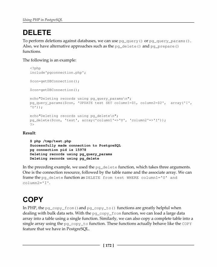
Using PHP in PostgreSQL

[ 172 ]

DELETETo perform deletions against databases, we can use pg_query() or pg_query_params().Also, we have alternative approaches such as the pg_delete() and pg_prepare()functions.

The following is an example:

<?phpinclude'pgconnection.php';

$con=getDBConnection();

$con=getDBConnection();

echo"Deleting records using pg_query_params\n";pg_query_params($con, 'UPDATE test SET column1=$1, column2=$2', array('I','U'));

echo"Deleting records using pg_delete\n";pg_delete($con, 'test', array('column1'=>'U', 'column2'=>'I'));?>

Result:

$ php /tmp/test.phpSuccessfully made connection to PostgreSQLpg connection pid is 15978Deleting records using pg_query_paramsDeleting records using pg_delete

In the preceding example, we used the pg_delete function, which takes three arguments.One is the connection resource, followed by the table name and the associate array. We canframe the pg_delete function as DELETE from test WHERE column1='U' andcolumn2='I'.

COPYIn PHP, the pg_copy_from()and pg_copy_to() functions are greatly helpful whendealing with bulk data sets. With the pg_copy_from function, we can load a large dataarray into a table using a single function. Similarly, we can also copy a complete table into asingle array using the pg_copy_to function. These functions actually behave like the COPYfeature that we have in PostgreSQL.

Using PHP in PostgreSQL

[ 173 ]

The following is an example:

<?phpinclude'pgconnection.php';

$con=getDBConnection();

echo"Loading actual dummy table into an array\n";$rows = pg_copy_to($con, 'test');printf("Number of rows loaded into array is %ld\n", count($rows));

echo"Now loading the records to backup table\n";pg_copy_from($con, 'test_backup', $rows);

$res = pg_query($con, "SELECT COUNT(*) FROM test_backup");printf("Count of test table %ld\n", pg_fetch_result($res, 0, 0));?>

Result:

$ php /tmp/test.phpSuccessfully made connection to PostgreSQLpg connection pid is 32108Loading actual test table into an arrayNumber of rows loaded into array is 1048576Now loading the records to backup tableCount of test table 1048576

In the preceding example, we dump all the records of test table into the $rows array, andagain load the complete array into the dump_backup table using two simple function calls.

In PHP, we can also COPY from stdin using the pg_put_line and pg_end_copyfunctions.

Let's see an example of how to read data from stdin for the COPY statement:

<?php...$con=getDBConnection();pg_query($con, "COPY test FROM STDIN");pg_put_line("U\tI\n");pg_put_line("U\tI\n");pg_put_line("\\.\n");pg_end_copy();

$rows=pg_copy_to($con, 'test');print_r($rows);?>

Using PHP in PostgreSQL

[ 174 ]

Result:

$ php /tmp/test.phpSuccessfully made connection to PostgreSQLpg connection pid is 37913Array([0] => UI[1] => UI)

From the preceding results, we see the actual output of print_r($rows); it prints therecords using \t as the delimiter, which is the default PostgreSQL COPY statementdelimiter. This is the reason pg_copy_from works with the array that was returned by thepg_copy_to function.

SummaryIn this chapter, we used PHP with Postgres. We started with simple connections; however,we talked about the available PHP functions for DDL, DML and SELECT. For yourconvenience, we described each section with examples and provided PHP code that you cantest yourself. We hope that will give you a better understanding of PHP. We also hope that,after reading this chapter, you will be able to prepare PHP code and execute it on your own.In the next chapter, we will talk about Java with PostgreSQL. Java is one of the mostpopular programming languages in the market. So many applications are designed on Javaand connect to the database. We will use real-time examples to describe how and where it isuseful. Additionally, we will also cover how to create a table from PL/Java andaccess/modify it through the code.

11Using Java in PostgreSQL

In the previous chapter, we talked about how to make a connection to PostgreSQL usingPHP; the available PHP functions to modify the database objects using DMLs and DDLs;and functions to fetch the data using SELECTs. To understand this better, we even providedexamples. This gives you a basic idea about how to proceed with PHP if you want to buildcode based on it. In this chapter, we will make database connections using Java, which isone of the most popular programming languages in the technology world. Additionally, wewill also cover how to create objects using Java, and how to manipulate data once theobjects are created. We will provide some examples with sample codes, which will help youstart with it. We will also talk about Java Database Connectivity (JDBC) drivers that areneeded to run the Java code against databases.

Making database connections toPostgreSQL using JavaAs this book is intended to give you the basics, we will start with simple Java code thatretrieves data from the database. For the Java code, we should have Java installed on themachine, and we need a PosgreSQL java driver to connect it to the database.

Here is the sample code:

import java.sql.Connection;import java.sql.DriverManager;import java.sql.Statement;import java.sql.ResultSet;import java.sql.SQLException;

public class JavaSelect {

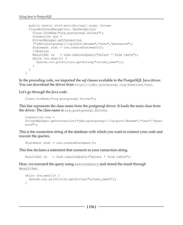
Using Java in PostgreSQL

[ 176 ]

public static void main(String[] args) throws ClassNotFoundException, SQLException{ Class.forName("org.postgresql.Driver"); Connection con = DriverManager.getConnection ("jdbc:postgresql://ip:port/dbname","user","password"); Statement stmt = con.createStatement(); //Queries ResultSet rs = stmt.executeQuery("select * from table"); while (rs.next()) { System.out.println(rs.getString("column_name")); } }}

In the preceding code, we imported the sql classes available in the PostgreSQL Java driver.You can download the driver from h t t p s : / / j d b c . p o s t g r e s q l . o r g / d o w n l o a d . h t m l.

Let's go through the Java code:

Class.forName("org.postgresql.Driver");

This line represents the class name from the postgresql driver. It loads the main class fromthe driver. The class name is org.postgresql.Driver.

Connection con =DriverManager.getConnection("jdbc:postgresql://ip:port/dbname","user","password");

This is the connection string of the database with which you want to connect your code andexecute the queries.

Statement stmt = con.createStatement();

This line declares a statement that connects to your connection string.

ResultSet rs = stmt.executeQuery("select * from table");

Here, we executed the query using executeQuery and stored the result throughResultSet.

while (rs.next()) { System.out.println(rs.getString("column_name"));}

Using Java in PostgreSQL

[ 177 ]

Here, we printed the output from the results stored.

Now, let's look at a real example. We have a table, java_test, in the postgres database,and we inserted a couple of rows:

postgres=# select * from java_test ;id---- 1 2(2 rows)

Now, we will retrieve this table from Java code. Here is the code:

import java.sql.Connection;import java.sql.DriverManager;import java.sql.Statement;import java.sql.ResultSet;import java.sql.SQLException;

public class JavaSelect { public static void main(String[] args) throws ClassNotFoundException, SQLException{ Class.forName("org.postgresql.Driver"); Connection con = DriverManager.getConnection ("jdbc:postgresql: //127.0.0.1:5432/postgres","postgres","postgres"); Statement stmt = con.createStatement(); //Queries ResultSet rs = stmt.executeQuery("select * from java_test");

while (rs.next()) { System.out.println(rs.getString("id")); } }}

We have to compile the code before executing it. As we are using Linux, javac is the Javacompiler:

root@ubuntu:/home/postgres# javac JavaStmtPG.java

Using Java in PostgreSQL

[ 178 ]

It creates a .class file that you can execute through Java. However, as we said, it needs aPostgreSQL Java driver to execute it. We downloaded thepostgresql-9.4.1208.jre6.jar driver for this demo. Here is how you can execute it:

root@ubuntu:/home/postgres# java -cp :postgresql-9.4.1208.jre6.jarJavaStmtPG12root@ubuntu:/home/postgres#

So, it executed the query in the database and printed the rows.

Using Java to create a PostgreSQL tableAs of now, we have explored a simple example to retrieve rows of a table with a singlecolumn. Now, lets's see how to create a table using Java.

We will use the same kind of code (with some modifications) to create the table. Here is thesample code:

import java.sql.Connection;import java.sql.DriverManager;import java.sql.Statement;import java.sql.ResultSet;import java.sql.SQLException;public class JavaCreate { public static void main(String[] args) throws ClassNotFoundException, SQLException{ Class.forName("org.postgresql.Driver"); Connection con = DriverManager.getConnection ("jdbc:postgresql: //127.0.0.1:5432/postgres","postgres","postgres"); Statement stmt = con.createStatement(); stmt = con.createStatement(); String sql = "CREATE TABLE demo_create " + "(ID INT PRIMARY KEY NOT NULL," + " FIRST_NAME VARCHAR NOT NULL, " + " LAST_NAME VARCHAR)"; stmt.executeUpdate(sql); stmt.close(); con.close(); System.out.println("Table created successfully"); }}

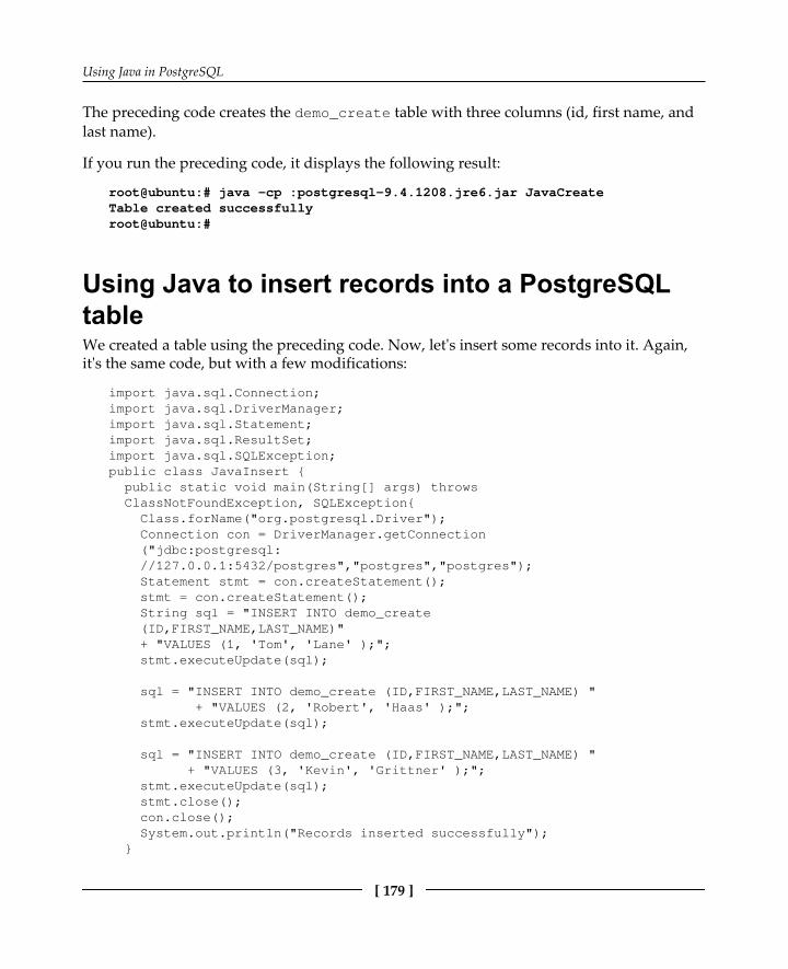
Using Java in PostgreSQL

[ 179 ]

The preceding code creates the demo_create table with three columns (id, first name, andlast name).

If you run the preceding code, it displays the following result:

root@ubuntu:# java -cp :postgresql-9.4.1208.jre6.jar JavaCreateTable created successfullyroot@ubuntu:#

Using Java to insert records into a PostgreSQLtableWe created a table using the preceding code. Now, let's insert some records into it. Again,it's the same code, but with a few modifications:

import java.sql.Connection;import java.sql.DriverManager;import java.sql.Statement;import java.sql.ResultSet;import java.sql.SQLException;public class JavaInsert { public static void main(String[] args) throws ClassNotFoundException, SQLException{ Class.forName("org.postgresql.Driver"); Connection con = DriverManager.getConnection ("jdbc:postgresql: //127.0.0.1:5432/postgres","postgres","postgres"); Statement stmt = con.createStatement(); stmt = con.createStatement(); String sql = "INSERT INTO demo_create (ID,FIRST_NAME,LAST_NAME)" + "VALUES (1, 'Tom', 'Lane' );"; stmt.executeUpdate(sql);

sql = "INSERT INTO demo_create (ID,FIRST_NAME,LAST_NAME) " + "VALUES (2, 'Robert', 'Haas' );"; stmt.executeUpdate(sql);

sql = "INSERT INTO demo_create (ID,FIRST_NAME,LAST_NAME) " + "VALUES (3, 'Kevin', 'Grittner' );"; stmt.executeUpdate(sql); stmt.close(); con.close(); System.out.println("Records inserted successfully"); }

Using Java in PostgreSQL

[ 180 ]

}

If you run the preceding code, it inserts three records in the demo_create table:

root@ubuntu:# java -cp :postgresql-9.4.1208.jre6.jar JavaInsertRecords inserted successfullyroot@ubuntu:# /opt/PostgreSQL/9.4/bin/psql -p 5432 -U postgres -d postgres-Aqt -c "select * from demo_create"Password for user postgres:1|Tom|Lane2|Robert|Haas3|Kevin|Grittner

Using Java to update records into a PostgreSQLtableAgain, to update/delete the rows from a table, you can use the same piece of code with afew modifications.

You can change the SQL statement in the preceding code to the following one for UPDATE:

String sql = "UPDATE demo_create SET ID=4 where ID=1;";stmt.executeUpdate(sql);

Here is the sample code for your convenience:

import java.sql.Connection;import java.sql.DriverManager;import java.sql.Statement;import java.sql.ResultSet;import java.sql.SQLException;

public class JavaUpdate { public static void main(String[] args) throws ClassNotFoundException, SQLException{ Class.forName("org.postgresql.Driver"); Connection con = DriverManager.getConnection ("jdbc:postgresql: //127.0.0.1:5432/postgres","postgres","postgres"); Statement stmt = con.createStatement(); stmt = con.createStatement(); String sql = "UPDATE demo_create SET ID=4 where ID=1;"; stmt.executeUpdate(sql); stmt.close(); con.close();

Using Java in PostgreSQL

[ 181 ]

System.out.println("Records updated successfully"); }}

This is the result when you compile and run it:

root@ubuntu:# javac JavaUpdate.javaroot@ubuntu:# java -cp :postgresql-9.4.1208.jre6.jar JavaUpdateRecords updated successfullyroot@ubuntu:# psql -p 5432 -d postgres -U postgres -c "select * fromdemo_create" id | first_name | last_name----+------------+----------- 2 | Robert | Haas 3 | Kevin | Grittner 4 | Tom | Lane(3 rows)

Using Java to delete records into a PostgreSQLtableSo far, we have created, inserted, and updated the table. Now, let's delete the rows from thetable. Again, we will use the same piece of code as an example:

import java.sql.Connection;import java.sql.DriverManager;import java.sql.Statement;import java.sql.ResultSet;import java.sql.SQLException;

public class JavaUpdate { public static void main(String[] args) throws ClassNotFoundException, SQLException{ Class.forName("org.postgresql.Driver"); Connection con = DriverManager.getConnection ("jdbc:postgresql: //127.0.0.1:5432/postgres","postgres","postgres"); Statement stmt = con.createStatement(); stmt = con.createStatement(); String sql = "DELETE FROM demo_create WHERE ID=2;"; stmt.executeUpdate(sql); stmt.close(); con.close(); System.out.println("Records Deleted successfully"); }

Using Java in PostgreSQL

[ 182 ]

}

Here is the output when you run the preceding piece of code:

root@ubuntu:# psql -p 5432 -d postgres -U postgres -c "select * fromdemo_create" id | first_name | last_name----+------------+----------- 2 | Robert | Haas 3 | Kevin | Grittner 4 | Tom | Lane(3 rows)

root@ubuntu:# javac JavaDelete.javaroot@ubuntu:# java -cp :postgresql-9.4.1208.jre6.jar JavaDeleteRecords Deleted successfullyroot@ubuntu:#root@ubuntu:# psql -p 5432 -d postgres -U postgres -c "select * fromdemo_create" id | first_name | last_name----+------------+----------- 2 | Robert | Haas 3 | Kevin | Grittner(2 rows)

Catching exceptionsSo far, we have examined at simple code that just executes statements, such as create, insert,delete, and update; however, we did not try to catch the exceptions.However, it is mostimportant that you catch code exceptions in the real world. Here is simple code to capturean exception using the try/catch block:

import java.sql.Connection;import java.sql.DriverManager;import java.sql.Statement;import java.sql.ResultSet;import java.sql.SQLException;

public class JavaConnection { public static void main(String args[]) { Connection conn = null; try { Class.forName("org.postgresql.Driver"); conn = DriverManager .getConnection("jdbc:postgresql:

Using Java in PostgreSQL

[ 183 ]

//127.0.0.1:5432/postgres","postgres", "postgres"); } catch (Exception exp_err) { exp_err.printStackTrace(); System.err.println(exp_err.getClass().getName()+": "+exp_err.getMessage()); System.exit(0); } System.out.println("Opened database successfully"); }}

The preceding example, captures connection errors if it is unable to connect to db.

For a successful connection:

root@ubuntu:# javac JavaConnection.javaroot@ubuntu:# java -cp :postgresql-9.4.1208.jre6.jar JavaConnectionOpened database successfullyroot@ubuntu:#

For a failed connection:

root@ubuntu:# javac JavaConnection.javaroot@ubuntu:# java -cp :postgresql-9.4.1208.jre6.jar JavaConnectionorg.postgresql.util.PSQLException: FATAL: database "postgrues" does notexist atorg.postgresql.core.v3.ConnectionFactoryImpl.readStartupMessages(ConnectionFactoryImpl.java:712) atorg.postgresql.core.v3.ConnectionFactoryImpl.openConnectionImpl(ConnectionFactoryImpl.java:213) atorg.postgresql.core.ConnectionFactory.openConnection(ConnectionFactory.java:66) at org.postgresql.jdbc.PgConnection.<init>(PgConnection.java:215) at org.postgresql.Driver.makeConnection(Driver.java:406) at org.postgresql.Driver.connect(Driver.java:274) at java.sql.DriverManager.getConnection(DriverManager.java:571) at java.sql.DriverManager.getConnection(DriverManager.java:215) at JavaConnection.main(JavaConnection.java:12)org.postgresql.util.PSQLException: FATAL: database "postgrues" does notexistroot@ubuntu:#

Using Java in PostgreSQL

[ 184 ]

Using prepared statementsPostgreSQL allows the server side to prepare statements. Its purpose is to reuse the parsingand planning of statements and reduce some overhead. Here is the sample code to usePreparedStatements in Java:

import java.sql.Connection;import java.sql.DriverManager;import java.sql.Statement;import java.sql.ResultSet;import java.sql.SQLException;import java.sql.PreparedStatement;

public class JavaPrepare { public static void main(String[] args) throws ClassNotFoundException, SQLException{ Class.forName("org.postgresql.Driver"); Connection con = DriverManager.getConnection ("jdbc:postgresql: //127.0.0.1:5432/postgres","postgres","postgres"); PreparedStatement stmt = con.prepareStatement("select * from demo_create"); ResultSet rs = stmt.executeQuery();

while (rs.next()) { System.out.println(rs.getString("id")); } }}

This is the output when you run the code:

root@ubuntu:# javac JavaPrepare.javaroot@ubuntu:# java -cp :postgresql-9.4.1208.jre6.jar JavaPrepare23root@ubuntu:#

Loading data using COPYTo improve data loading, PostgreSQL has a COPY command that loads/unloads the datafrom/to a file. You can load the data using COPY from JDBC using the CopyManagerconstructor. Here is an example:

import java.io.FileReader;

Using Java in PostgreSQL

[ 185 ]

import java.io.IOException;import java.sql.PreparedStatement;import java.sql.Connection;import java.sql.DriverManager;import java.sql.ResultSet;import java.sql.SQLException;import java.util.logging.Level;import java.util.logging.Logger;import org.postgresql.copy.CopyManager;import org.postgresql.core.BaseConnection;

public class JavaCopy { public static void main(String[] args) { try { Class.forName("org.postgresql.Driver"); Connection con = DriverManager.getConnection ("jdbc:postgresql: //127.0.0.1:5432/postgres","postgres","postgres"); CopyManager cm = new CopyManager((BaseConnection) con);

FileReader fr = new FileReader("test.txt"); cm.copyIn("COPY demo_create FROM STDIN WITH DELIMITER '|'", fr); } catch (Exception exp_err) { exp_err.printStackTrace(); System.err.println(exp_err.getClass().getName()+": "+exp_err.getMessage()); System.exit(0); } System.out.println("Copied data successfully"); }}

This is the output when you run the code:

root@ubuntu:~# psql -p 5432 -d postgres -U postgres -c "delete fromdemo_create"DELETE 3root@ubuntu:~# psql -p 5432 -d postgres -U postgres -c "select * fromdemo_create" id | first_name | last_name----+------------+-----------(0 rows)

root@ubuntu:~# cat test.txt1 | Robert | Haas2 | Tom | Lane3 | Kevin | Grittner

Using Java in PostgreSQL

[ 186 ]

root@ubuntu:~#root@ubuntu:~#root@ubuntu:~# javac -cp postgresql-9.4.1208.jre6.jar JavaCopy.javaroot@ubuntu:~# java -cp :postgresql-9.4.1208.jre6.jar JavaCopyCopied data successfullyroot@ubuntu:~#root@ubuntu:~#root@ubuntu:~# psql -p 5432 -d postgres -U postgres -c "select * fromdemo_create" id | first_name | last_name----+------------+----------- 1 | Robert | Haas 2 | Tom | Lane 3 | Kevin | Grittner(3 rows)

Connection propertiesLet's talk about the connection properties. While connecting to the database using theconnection string, as in the earlier examples, you can also set other parameters in additionto standard connection parameters. These properties may be specified in either theconnection URL or the additional properties object parameter toDriverManager.getConnection. The following examples illustrate the use of bothmethods to establish an SSL connection:

String url = "jdbc:postgresql://localhost/postgres";Properties props = new Properties();props.setProperty("user","fred");props.setProperty("password","secret");props.setProperty("ssl","true");Connection conn = DriverManager.getConnection(url, props);

or

String url ="jdbc:postgresql://localhost/test?user=fred&password=secret&ssl=true";Connection conn = DriverManager.getConnection(url);

You can go through the driver documentation ( h t t p s : / / j d b c . p o s t g r e s q l . o r g / d o c u m e n t a

t i o n / 9 3 / c o n n e c t . h t m l # c o n n e c t i o n - p a r a m e t e r s) for details of more available connectionparameters.

Using Java in PostgreSQL

[ 187 ]

SummaryIn this chapter, we talked about making a connection to databases using Java and, once thatconnection is established, we talked about creating objects and inserting/updating/deletingdata from the objects with simple examples, which helps you understand easily and writethe required Java code. We covered not only simple executions but also catching exceptionswhen code fails to run, which gives you a hint to further troubleshooting. We also talkedabout prepared statements, which reduce the overhead of parsing/planning on the server,and loading the data using COPY, which is a faster way to load data in PostgreSQL.

Index

Aanomalies, DBMS common patterns 64 delete anomaly 61 first normal form (1NF) 62 insert anomaly 61 second normal form (2NF) 62 third normal form (3NF) 63 update anomaly 61ANSI isolation levels explicit transaction, using 76 implicit transaction, using 76 isolation level, changing 75 transaction isolation levels 75array constructors about 29 ARRAY_AGG() 32 array_dims() 32 Array_length() 34 ARRAY_UPPER() 34 string_t0-array() 31array about 28 constructors 28 JSON 37 slicing 34 splicing 34 UNNESTing, to rows 35 XML, using in PostgreSQL 41Atomicity, Consistency, Isolation, and Durability

(ACID) atomicity 69 consistency 70 durability 70 isolation 70

Bbinary large objects creating 154 data, writing to 155 exporting 155 importing 154 server-side functions 155 using 153Block Range Index (BRIN) about 90 reference link 90

Ccache, cleaning pg_buffercache extensions, using 127, 128 pg_prewarm extensions, using 129cached data optimizer setting 130, 132chunks 153common patterns hierarchy 65 many-to-many relationships 64 recursive relationships 66composite datatype about 42 altering, in PostgreSQL 44 creating, in PostgreSQL 42 dropping, in PostgreSQL 45connection properties 186constraint exclusion about 107, 114, 115, 116 foreign inheritance 118, 120 horizontal partitioning 116 PL/Proxy 117constraints about 81

[ 189 ]

check constraint 95 check constraints 94 exclusion constraints 96 foreign key constraint 91 NOT NULL constraints 95 unique constraints 92, 93COPY command used, for loading data 184count function reference link 13cursors about 10 closing 12 creating 10, 11 using 11

DData Manipulation Language (DML) 8, 81datatypes conversion between 27DBMS anomalies 60DDLs dealing with 161design rules data efficiency imposing ability 59 data integrity imposing ability 59 future changes accommodation ability 60 problem solving ability 58 relationship support ability 59 required data holding ability 59DML operation executing 162 pg_insert function 164 pg_query_params function 163driver documentation reference link 186

Eexclusion constraints 96execution plan 141explain plan complex example 142 generating 141 reading 141

running 141 simple example 142explicit locking about 77 rows, locking 77 tables, locking 79extension compiling 149, 150 creating 147, 148, 149

Ffirst normal form (1NF) 62full text search reference link 86

GGeneralized Inverted Index (GIN) 86Generalized Search Tree (GiST) 86GROUP BY clause using 12

HHAVING clause arguments 14 parameters 14 using 14helper functions COPY function 172 DELETE function 172 pg_convert function 169 pg_field_name function 168 pg_free_results function 168 pg_meta_data function 168 pg_num_fields function 168 pg_num_rows functions 168 UPDATE function 171 used, for dealing with data fetching 168

Iindex about 81 B-Tree indexes 84 clustering 90, 91 full text indexes 86

[ 190 ]

GIN 89 GiST indexes 89 hash indexes 89 multicolumn indexes 88 partial indexes 86 primary key indexes 82, 83 standard indexes 85 unique indexes 83, 84isolation levels, transaction dirty reads 72 phantom reads 74 unrepeatable reads 73

JJava Database Connectivity (JDBC) 175Java exceptions, catching 182 used, for creating PostgreSQL table 178 used, for deleting records into PostgreSQL table

181

used, for inserting records into PostgreSQL table 179

used, for making database connections toPostgreSQL 175, 177

used, for updating records into PostgreSQL table 180

JSON, querying containment 38 equality operations 38 key/element existence 39 output, obtaining 40JSON about 37 data, inserting in PostgreSQL 37 querying 38

LLIMIT clause using 15

MManage External Data (MED) 118materialized views about 8 benefits 8

read-only 8, 9 updatable 8, 9, 10 writeable 8, 10max function reference link 13min function reference link 13

Nnormalization 60

Ooptimizer setting for cached data 130, 132Outer join about 22 full outer join 25 Left outer join 23 right outer join 24 types 22

Ppartitioning about 101 alternate methods 111, 112, 113 list partition 107 types 107partitions adding 109 implementing, on table 102, 103, 104, 105, 106 managing 109 old partition, purging 110persistent connections reference link 158pg_partman extension reference link 111pg_query_params functions reference link 163PHP-to-PostgreSQL connections creating 158PL/Proxy reference link 117PosgreSQL databases connections, making with Java 175PostGIS Install Guide

[ 191 ]

reference link 150PostgreSQL 9.5.3 Documentation reference link 127PostgreSQL Java driver reference link 176PostgreSQL table creating, with Java 178, 179 records, deleting with Java 181 records, inserting with Java 179 records, updating with Java 180PostgreSQL about 5 composite types, altering 44 composite types, creating 42 database links 150, 152, 153 databases connections, making with Java 177 documentation, reference link 155 JSON data, inserting 37 triggers, adding 47 triggers, modifying 52 using, with PHP 157 XML data, inserting 41 XML, using 41prepared statements data, loading with COPY 184 using 184psql 11

Qquery operators about 143 Aggregate operator 144 Append operator 144 Group operator 145 Hash Join operator 145 Hash operator 145 Index Scan operator 143 Limit operator 144 Materialize operator 146 Merge Join operator 145 Nested Loop operator 145 Result operator 144 SeqScan operator 143 Setop operator 146 Sort operator 144

Subquery Scan operator 145 Tid Scan operator 145 Unique operator 144query tuning about 122 cache, cleaning 126, 127 cache, tuning 124 hot, versus cold cache 123query implementing, multiple ways 132

Rrecords, retrieving about 165 pg_fetch_all, using 165 pg_fetch_assoc function, using 166 pg_fetch_result function, using 167

Sscalar subquery 17second normal form (2NF) 62self join about 21 using 22stale statistics optimizer hints 136, 140 Optimizer hints 138 used, for bad query performance 134, 136subqueries arguments 19 correlated subqueries 18 existence subqueries 19 parameters 19 used, for returning multiple rows 18 using 16sum function reference link 13, 14

Ttable partitioning 97, 98, 101third normal form (3NF) 63transaction isolation about 72 levels, implementing 72transactions

and savepoints 71 ANSI isolation levels 74 Atomicity, Consistency, Isolation, and Durability

(ACID) 69 concurrency, effects 70 deadlocks, avoiding 76 defining 68 explicit locking 77 isolation 72trigger function creating 54 testing 55triggers about 46 adding, to PostgreSQL 47 existing triggers, viewing 56 modifying, in PostgreSQL 52 removing 53

U

Union join using 20, 21UPDATE operation clauses using 15

Vviews about 5 creating 5 creating, commands 6 deleting 7 replacing 7

XXML data, inserting in PostgreSQL 41 data, querying 42 using, in PostgreSQL 41