sensors

Article

Wearable Devices for Classification of InadequatePosture at Work Using Neural Networks

Eya Barkallah 1, Johan Freulard 1, Martin J. -D. Otis 1, Suzy Ngomo 2, Johannes C. Ayena 1,* andChristian Desrosiers 3

1 Laboratory of Automation and 3D Multimodal Intelligent Interaction (LAIMI),Department of Applied Sciences, University of Quebec at Chicoutimi (UQAC),555 Boulevard de l’Université, Chicoutimi, QC G7H 2B1, Canada; eya.barkallah1@uqac.ca (E.B.);johan.freulard1@uqac.ca (J.F.); martin_otis@uqac.ca (M.J.-D.O.)

2 Laboratory of Automation and 3D Multimodal Intelligent Interaction (LAIMI),Department of Health Sciences, University of Quebec at Chicoutimi (UQAC), 555 Boulevard de l’Université,Chicoutimi, QC G7H 2B1, Canada; suzy_ngomo@uqac.ca

3 Department of Software and IT Engineering, École de Technologie Supérieure (ÉTS),1100 Rue Notre-Dame Ouest, Montreal, QC H3C 1K3, Canada; christian.desrosiers@etsmtl.ca

* Correspondence: cossoun-johannes.ayena1@uqac.ca; Tel.: +1-418-545-5011

Received: 31 July 2017; Accepted: 30 August 2017; Published: 1 September 2017

Abstract: Inadequate postures adopted by an operator at work are among the most important riskfactors in Work-related Musculoskeletal Disorders (WMSDs). Although several studies have focusedon inadequate posture, there is limited information on its identification in a work context. The aimof this study is to automatically differentiate between adequate and inadequate postures usingtwo wearable devices (helmet and instrumented insole) with an inertial measurement unit (IMU)and force sensors. From the force sensors located inside the insole, the center of pressure (COP) iscomputed since it is considered an important parameter in the analysis of posture. In a first step, a setof 60 features is computed with a direct approach, and later reduced to eight via a hybrid featureselection. A neural network is then employed to classify the current posture of a worker, yielding arecognition rate of 90%. In a second step, an innovative graphic approach is proposed to extract threeadditional features for the classification. This approach represents the main contribution of this study.Combining both approaches improves the recognition rate to 95%. Our results suggest that neuralnetwork could be applied successfully for the classification of adequate and inadequate posture.

Keywords: posture; center of pressure; instrumented insole; IMU; supervised classification; featureselection; neural networks

1. Introduction

Several studies, summarized by da Costa et al. [1], have reported that Work-related MusculoskeletalDisorders (WMSDs) generally result from repetitive movements and prolonged or inadequate postures.Pain is the main WMSD symptom, although they may also be accompanied with abnormal motor patternssuch as movement deficits (elevation, rotation, etc.) [2] and lack of strength [3], both of which can lead towork disability. Worldwide, the magnitude and prevalence of WMSDs represent a public health concernencountered in most industrialized societies [4–8]. Thus, over 40 million workers in Europe are affectedby MSDs attributable to their work [9]. In the province of Ontario (Canada), based on population dataof 45,650 individuals aged 16 years and over, MSDs were mentioned as a reason for 40% of all chronicconditions, 54% of all long-term disabilities, 24% of restricted activity days, and almost 20% of health careutilization [4]. The impact of MSDs was even greater in the 65 and over age group [5,10]. According to theCommittee on Standards, Equity of Occupational Health and Safety of Quebec (CSEOHS), the number

Sensors 2017, 17, 2003; doi:10.3390/s17092003 www.mdpi.com/journal/sensors

Sensors 2017, 17, 2003 2 of 24

of WMSD lesions affecting workers between 2012 and 2015 represented approximately 27% of the casesclaimed, disregarding the non-reported cases [11]. Furthermore, MSDs are responsible for morbidity inmany working population and are known as an important occupational problem with increasing healthcosts. In the last past decade, MSD-related costs were estimated at around 17 billion pounds in the UK,38 billion euros in Germany, 215 billion dollars in the US, and 26 billion Canadian dollars [12]. Therefore,there is a critical need to introduce effective detection solutions of inadequate postures which may lead toWMSD in the industry.

WMSD detection often focuses on monitoring ergonomic risk factors by self-report questionnairesand/or by direct or indirect observational methods [13,14]. However, it is unclear why on asimilar workstation, a person will develop a MSD while another will not. Thus, identifyingthe personal determinants of MSD development remains a challenge, and a better detection ofwork-related risk factors is still an important issue [13]. The use of electronic assessment tools seemsto be the most promising solution for successful detection [15]. Various technologies, such as 3Dmotion analysis, have been exploited to gain a more objective or quantitative indication of workerposture and movements [16–18]. However, camera-based systems require considerable workspace ortime-consuming calibration operations, and their costs are usually quite high. The most commonly useddevice to analyze human posture is the force platform, which measures displacements of the center ofpressure (COP) [19]. COP is defined as the point location of the vertical ground reaction, and is oftenused to identify a balance deficit [20]. Although these measures are reliable and valid, force platformsystems are expensive and reduce the ability to detect in real time the quantitative parameters of posturesin real work environment [21,22]. Furthermore, the subject is limited in movements (a quasi-staticposition). Another approach consists in using sensors attached to the worker for collecting datarelated to this worker’s own exposure variables [23–25]. A possible shortcoming of this approach is itsencumbrance, weight, and lack of portability, which limit its use in work activities. For body motionsstudies, there is a trend towards combining observational approaches with direct recording methodsthat use instrumentation [18,26]. While combining several detection procedures in a multidisciplinaryapproach should provide better results than using a single procedure, it is unclear how to combinethem for optimal results. Also, implementing these combinations can take a lot of time.

Thereby, in this study, we focus on the design of an effective measurement system fordifferentiating automatically adequate and inadequate postures. As an electronic and automaticassessment tool, we first introduce an enactive insole and smart helmet as wearable devices to betteranalyze workers’ posture. Since posture analysis can be both an expensive and time-consuming process,previous studies have underlined the need for automatic models that can detect inadequate posture [27].Some researchers have demonstrated the relevance of advanced statistical methods such as logisticregression [28], Bayesian models [29], artificial neural networks (ANN) [30] or K-nearest neighbor(KNN) algorithms [31] to predict the risk associated with occupational exposures. These methodshave produced varying prediction accuracy, depending on the task factors examined and the qualityof the data used for model development. In many cases, neural networks have been shown to yieldsuperior predictive accuracy compared to, for example, multiple linear regression models [32,33].This could be attributed to the ability of ANNs to model complex and nonlinear relationships betweenvariables [34]. It may also be due to the fact that the statistical methods investigated have rigidassumptions associated with the nature of the data (e.g., linearity, normality, homogeneity of variance),whereas, neural networks make no such assumptions [35]. Thus, we hypothesized that an ANNmodel could determine effectively the posture of a person in a real working environment, with easilymeasurable clinical variables such as the COP.

The main contribution of the present study is to develop a new methodology for classifying thecurrent posture of workers using the developed instrumentation. More specifically, we establish a newtype of features, related to the COP and inertial measurement unit (IMU) data, to classify posturesat workstations. To achieve this goal, we focus on prolonged or inadequate postures, since those can

Sensors 2017, 17, 2003 3 of 24

constitute a personal determinant of WMSD-related risk. The proposed classification algorithm isoptimized by using a hybrid feature selection method.

2. Design of the Measurement System

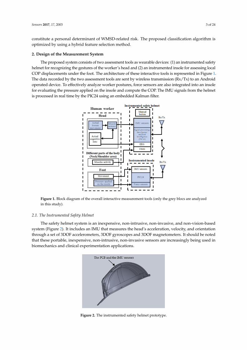
The proposed system consists of two assessment tools as wearable devices: (1) an instrumented safetyhelmet for recognizing the gestures of the worker’s head and (2) an instrumented insole for assessing localCOP displacements under the foot. The architecture of these interactive tools is represented in Figure 1.The data recorded by the two assessment tools are sent by wireless transmission (Rx/Tx) to an Androidoperated device. To effectively analyze worker postures, force sensors are also integrated into an insolefor evaluating the pressure applied on the insole and compute the COP. The IMU signals from the helmetis processed in real time by the PIC24 using an embedded Kalman filter.

Figure 1. Block diagram of the overall interactive measurement tools (only the grey blocs are analyzedin this study).

2.1. The Instrumented Safety Helmet

The safety helmet system is an inexpensive, non-intrusive, non-invasive, and non-vision-basedsystem (Figure 2). It includes an IMU that measures the head’s acceleration, velocity, and orientationthrough a set of 3DOF accelerometers, 3DOF gyroscopes and 3DOF magnetometers. It should be notedthat these portable, inexpensive, non-intrusive, non-invasive sensors are increasingly being used inbiomechanics and clinical experimentation applications.

Sensors 2017, 17, 2003 3 of 24

2. Design of the Measurement System

The proposed system consists of two assessment tools as wearable devices: (1) an instrumented safety helmet for recognizing the gestures of the worker’s head and (2) an instrumented insole for assessing local COP displacements under the foot. The architecture of these interactive tools is represented in Figure 1. The data recorded by the two assessment tools are sent by wireless transmission (Rx/Tx) to an Android operated device. To effectively analyze worker postures, force sensors are also integrated into an insole for evaluating the pressure applied on the insole and compute the COP. The IMU signals from the helmet is processed in real time by the PIC24 using an embedded Kalman filter.

Figure 1. Block diagram of the overall interactive measurement tools (only the grey blocs are analyzed in this study).

2.1. The Instrumented Safety Helmet

The safety helmet system is an inexpensive, non-intrusive, non-invasive, and non-vision-based system (Figure 2). It includes an IMU that measures the head’s acceleration, velocity, and orientation through a set of 3DOF accelerometers, 3DOF gyroscopes and 3DOF magnetometers. It should be noted that these portable, inexpensive, non-intrusive, non-invasive sensors are increasingly being used in biomechanics and clinical experimentation applications.

Figure 2. The instrumented safety helmet prototype.

The accelerometer adopted and used in the experimental trials of this work is the MPU9250 from TDK InvenSense (San Jose, CA, USA).

Figure 2. The instrumented safety helmet prototype.

Sensors 2017, 17, 2003 4 of 24

The accelerometer adopted and used in the experimental trials of this work is the MPU9250 fromTDK InvenSense (San Jose, CA, USA).

2.2. Enactive Insole Design

Worker posture can be analyzed by the COP’s displacement under the foot. This displacementis a virtual site of the plantar surface (Figure 3). More precisely, it is the average location of all thepressures acting on the foot at any given time [36]. Numerous studies [37,38] have examined COPdisplacements to assess and understand postural control during quiet stance or gait [39]. We havechosen to evaluate the posture and movement of the operator using the COPs positions (barycenter)computed as follows [40,41]:

XCOP =∑n

i=1 XiPi

∑ni=1 Pi

and YCOP =∑n

i=1 YiPi

∑ni=1 Pi

(1)

where n denotes the total number of sensors, i denotes a certain sensor, Pi is the pressure measured onsensor i, and Xi, Yi are the COP’s coordinates for sensor i inside the insole.

Sensors 2017, 17, 2003 4 of 24

2.2. Enactive Insole Design

Worker posture can be analyzed by the COP’s displacement under the foot. This displacement is a virtual site of the plantar surface (Figure 3). More precisely, it is the average location of all the pressures acting on the foot at any given time [36]. Numerous studies [37,38] have examined COP displacements to assess and understand postural control during quiet stance or gait [39]. We have chosen to evaluate the posture and movement of the operator using the COPs positions (barycenter) computed as follows [40,41]: X = ∑ X P∑ P and Y = ∑ Y P∑ P (1)

where n denotes the total number of sensors, i denotes a certain sensor, Pi is the pressure measured on sensor i, and Xi, Yi are the COP’s coordinates for sensor i inside the insole.

Figure 3. The prototype of the enactive insole with the preferred sensor location (the vibrating motor having the function of a rhythmic pattern is not used in this study).

From these measurements, the challenge is to classify the actual worker’s posture (and movement) into one of several predefined groups of postures (and movements), known as being either adequate or inadequate. To find the COP, we suggest one insole containing four force sensors (Figure 3). Several studies cited in [42,43] have shown that COP does not differ between dominant and non-dominant limbs. It was symmetric in young and healthy adults. Thus, we think that a single insole placed on the right foot (the foot we have chosen as usually the dominant foot of participant) could measure the COP positions in order to acquire the features we need for posture classification. In other studies related to the computation of the risk of fall, we also use only one enactive insole (located on the dominant limb) with successful results [44]. All this makes it possible to reduce the production cost of the device and use a minimal configuration and architecture (already presented in two other studies [45,46]). This allows the classification of the postures, not to optimize this configuration. This system is mainly designed for a long-term monitoring of worker and not for a diagnostic aid tool. Moreover, this system is not adapted for a clinical experimentation or clinical research.

Three sensors could also be used in our proposed insole, however the whole surface under the foot would not be covered. To determine the coordinates of the COP in the anteroposterior (YCOP) and mediolateral (XCOP) directions, we can use the data provided by the four force sensors located in our instrumented insole according to Equation (1). We begin the next subsection by comparing four types of force sensor technologies. Then, a characterization of several types of conductive supports is performed.

2.2.1. Comparison of Force Sensor Technologies

It is known that the force sensing resistor (FSR) sensor allows measuring the center of pressure parameters [41] using Equation (1). Based on previous research works in this field, the number of

Figure 3. The prototype of the enactive insole with the preferred sensor location (the vibrating motorhaving the function of a rhythmic pattern is not used in this study).

From these measurements, the challenge is to classify the actual worker’s posture (and movement)into one of several predefined groups of postures (and movements), known as being either adequateor inadequate. To find the COP, we suggest one insole containing four force sensors (Figure 3). Severalstudies cited in [42,43] have shown that COP does not differ between dominant and non-dominantlimbs. It was symmetric in young and healthy adults. Thus, we think that a single insole placed on theright foot (the foot we have chosen as usually the dominant foot of participant) could measure the COPpositions in order to acquire the features we need for posture classification. In other studies relatedto the computation of the risk of fall, we also use only one enactive insole (located on the dominantlimb) with successful results [44]. All this makes it possible to reduce the production cost of the deviceand use a minimal configuration and architecture (already presented in two other studies [45,46]).This allows the classification of the postures, not to optimize this configuration. This system is mainlydesigned for a long-term monitoring of worker and not for a diagnostic aid tool. Moreover, this systemis not adapted for a clinical experimentation or clinical research.

Three sensors could also be used in our proposed insole, however the whole surface under thefoot would not be covered. To determine the coordinates of the COP in the anteroposterior (YCOP) andmediolateral (XCOP) directions, we can use the data provided by the four force sensors located in ourinstrumented insole according to Equation (1). We begin the next subsection by comparing four types offorce sensor technologies. Then, a characterization of several types of conductive supports is performed.

Sensors 2017, 17, 2003 5 of 24

2.2.1. Comparison of Force Sensor Technologies

It is known that the force sensing resistor (FSR) sensor allows measuring the center of pressureparameters [41] using Equation (1). Based on previous research works in this field, the number ofsensors to compare is high. Therefore, this study only compared three sensors to a FSR sensor thatcan be added inside a very thin insole. This allowed us to optimize the current consumption in ourproposed insole device.

• The capacitive force sensor (CS8-100N, SingleTact, Los Angeles, CA, USA) has the same shape asthe FSR sensor. It is ultra-thin, thus allowing its integration in an instrumented insole withoutany issues. Its consumption is estimated at 2.5 mA according to its specifications [47], which israther high for a long term usage. Another disadvantage is that it costs three times more than theFSR sensor. Since the target price is around hundred dollars, lower-cost sensors (less or equal toten dollars each) were investigated.

• Various studies have also investigated the use of an optical sensor [48–51]. To exploit this sensorfor an instrumented insole, we need to integrate a light-emitting diode (LED), a phototransistorand a flexible structure that can introduce an obstruction between the LED and the phototransistor.The load over the structure adjusts the obstruction. The main issue of this technology is the currentconsumption of the light source, which still needs some improvements.

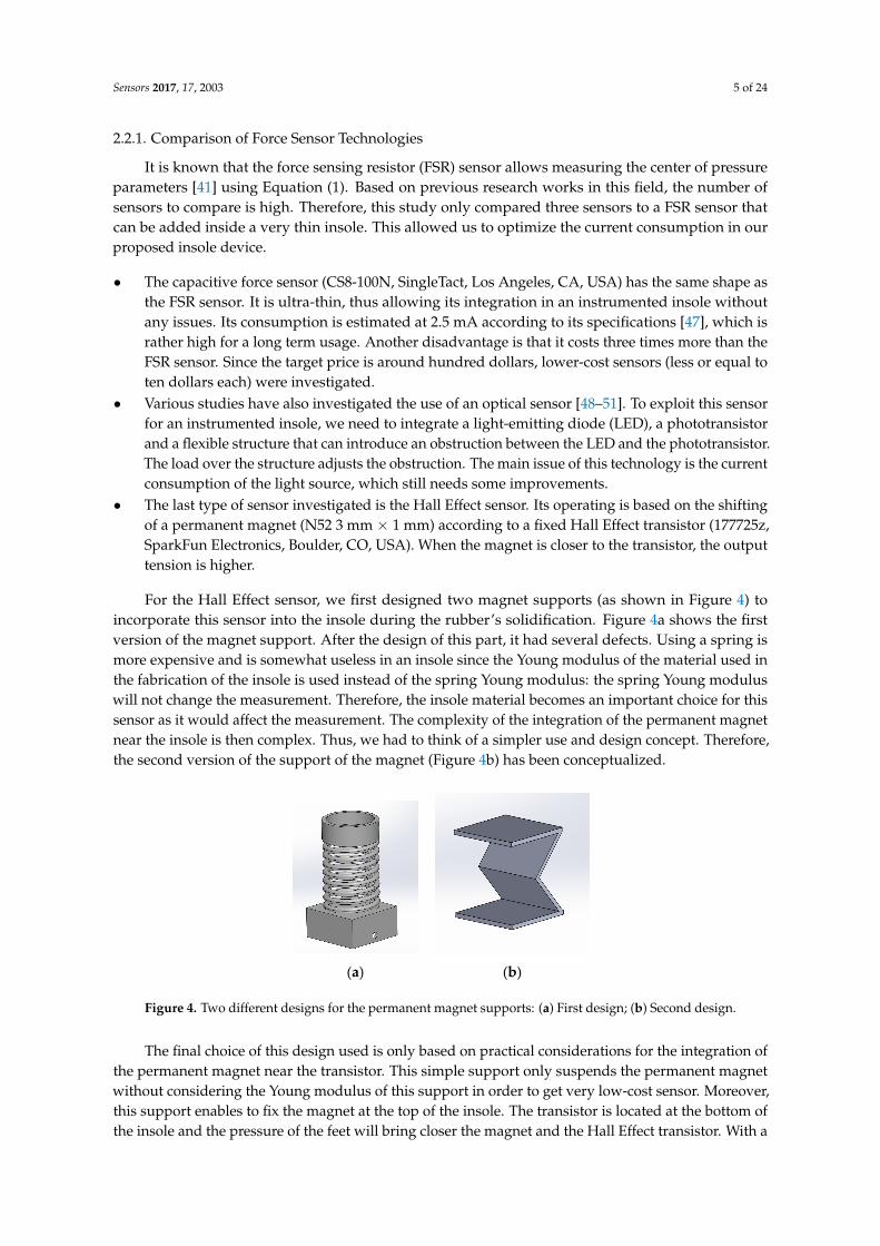
• The last type of sensor investigated is the Hall Effect sensor. Its operating is based on the shiftingof a permanent magnet (N52 3 mm × 1 mm) according to a fixed Hall Effect transistor (177725z,SparkFun Electronics, Boulder, CO, USA). When the magnet is closer to the transistor, the outputtension is higher.

For the Hall Effect sensor, we first designed two magnet supports (as shown in Figure 4) toincorporate this sensor into the insole during the rubber’s solidification. Figure 4a shows the firstversion of the magnet support. After the design of this part, it had several defects. Using a spring ismore expensive and is somewhat useless in an insole since the Young modulus of the material used inthe fabrication of the insole is used instead of the spring Young modulus: the spring Young moduluswill not change the measurement. Therefore, the insole material becomes an important choice for thissensor as it would affect the measurement. The complexity of the integration of the permanent magnetnear the insole is then complex. Thus, we had to think of a simpler use and design concept. Therefore,the second version of the support of the magnet (Figure 4b) has been conceptualized.

Sensors 2017, 17, 2003 5 of 24

sensors to compare is high. Therefore, this study only compared three sensors to a FSR sensor that can be added inside a very thin insole. This allowed us to optimize the current consumption in our proposed insole device.

The capacitive force sensor (CS8-100N, SingleTact, Los Angeles, CA, USA) has the same shape as the FSR sensor. It is ultra-thin, thus allowing its integration in an instrumented insole without any issues. Its consumption is estimated at 2.5 mA according to its specifications [47], which is rather high for a long term usage. Another disadvantage is that it costs three times more than the FSR sensor. Since the target price is around hundred dollars, lower-cost sensors (less or equal to ten dollars each) were investigated.

Various studies have also investigated the use of an optical sensor [48–51]. To exploit this sensor for an instrumented insole, we need to integrate a light-emitting diode (LED), a phototransistor and a flexible structure that can introduce an obstruction between the LED and the phototransistor. The load over the structure adjusts the obstruction. The main issue of this technology is the current consumption of the light source, which still needs some improvements.

The last type of sensor investigated is the Hall Effect sensor. Its operating is based on the shifting of a permanent magnet (N52 3 mm × 1 mm) according to a fixed Hall Effect transistor (177725z, SparkFun Electronics, Boulder CO, USA). When the magnet is closer to the transistor, the output tension is higher.

For the Hall Effect sensor, we first designed two magnet supports (as shown in Figure 4) to incorporate this sensor into the insole during the rubber’s solidification. Figure 4a shows the first version of the magnet support. After the design of this part, it had several defects. Using a spring is more expensive and is somewhat useless in an insole since the Young modulus of the material used in the fabrication of the insole is used instead of the spring Young modulus: the spring Young modulus will not change the measurement. Therefore, the insole material becomes an important choice for this sensor as it would affect the measurement. The complexity of the integration of the permanent magnet near the insole is then complex. Thus, we had to think of a simpler use and design concept. Therefore, the second version of the support of the magnet (Figure 4b) has been conceptualized.

(a) (b)

Figure 4. Two different designs for the permanent magnet supports: (a) First design; (b) Second design.

The final choice of this design used is only based on practical considerations for the integration of the permanent magnet near the transistor. This simple support only suspends the permanent magnet without considering the Young modulus of this support in order to get very low-cost sensor. Moreover, this support enables to fix the magnet at the top of the insole. The transistor is located at the bottom of the insole and the pressure of the feet will bring closer the magnet and the Hall Effect transistor. With a preliminary calibration, we were able to have an operational sensor. However, before the insole design, different tests were done with an elastomer insole four millimeters thick. The Hall Effect transistor was realized with a 1 mm diameter magnet. The output voltages of this transistor (Figure 5) are no better than those of a 3 mm diameter magnet due to its smaller measuring range.

Figure 4. Two different designs for the permanent magnet supports: (a) First design; (b) Second design.

The final choice of this design used is only based on practical considerations for the integration ofthe permanent magnet near the transistor. This simple support only suspends the permanent magnetwithout considering the Young modulus of this support in order to get very low-cost sensor. Moreover,this support enables to fix the magnet at the top of the insole. The transistor is located at the bottom ofthe insole and the pressure of the feet will bring closer the magnet and the Hall Effect transistor. With a

Sensors 2017, 17, 2003 6 of 24

preliminary calibration, we were able to have an operational sensor. However, before the insole design,different tests were done with an elastomer insole four millimeters thick. The Hall Effect transistorwas realized with a 1 mm diameter magnet. The output voltages of this transistor (Figure 5) are nobetter than those of a 3 mm diameter magnet due to its smaller measuring range.Sensors 2017, 17, 2003 6 of 24

Figure 5. Output voltage of Hall effect sensor with a one millimeter magnet.

Secondly, in Figure 6, we compared our integrated Hall Effect sensor to the FSR sensor built with different resistors. The current consumption could be reduced on the FSR sensor with a higher resistor for the voltage divider, which gets saturated earlier.

Figure 6. Graphic of force sensors measures with different FSR’s resistor compared to a Hall Effect sensor.

We note the saturation around 2000 Pa with the Hall Effect sensor and the FSR sensor at 10 kΩ. However, the saturation limit is reached earlier as soon as we increase the resistor for reducing the current consumption. Our measurements suggest the use of a 10 kΩ resistor even if its current consumption is higher (up to 3.3 V). At this resistor value (10 kΩ), the FSR sensor consumes maximally 0.33 mA while the Hall Effect sensor consumes 2.3 mA (Figure 7). Due to its higher consumption, the Hall Effect sensor could not replace the FSR sensor in our system. For this study, we did not find a LED with consumption under 0.33 mA producing enough light to be used. However, a cluster of micro LED or carbon nanotubes are next-generation light sources that could eventually be used in our application. Thus, the FSR seems to be the best to use for our measurement system design (Figure 3).

Y = (-7x10-12)X3 + (8x10-9)X2 + (2x10-4)XR² = 0.9255

-0.1

0.0

0.1

0.2

0.3

0.4

0.5

0.6

0 500 1000 1500 2000 2500 3000 3500

Out

put V

olta

ge (V

)

Pressure apply on the insole (Pa)

Hall Effect sensor

Y = (3x10-10)X3- (3x10-6)X2 + (62x10-4)X -1.5646

R² = 0.9361

Y = (-10-11)X3 + (4x10-9)X2 + (4x10-4)X

R² = 0.9649

Y = (6x10-10)X3 - (4x10-6)X2 + (85x10-4)X - 2.5424

R² = 0.9461

Y = (5x10-10)X3 - (4x10-6)X2 + (104x10-4)X - 5.9776

R² = 0.9839

0.0

0.5

1.0

1.5

2.0

2.5

3.0

3.5

0 500 1000 1500 2000 2500 3000 3500

Sens

ors

outp

ut v

olta

ge (V

)

Pressure apply on the insole (Pa)FSR force sensor with a 68kΩ resistor Hall Effect sensorFSR force sensor with a 20kΩ resistor FSR force sensor with a 10kΩ resistor

Figure 5. Output voltage of Hall effect sensor with a one millimeter magnet.

Secondly, in Figure 6, we compared our integrated Hall Effect sensor to the FSR sensor built withdifferent resistors. The current consumption could be reduced on the FSR sensor with a higher resistorfor the voltage divider, which gets saturated earlier.

Sensors 2017, 17, 2003 6 of 24

Figure 5. Output voltage of Hall effect sensor with a one millimeter magnet.

Secondly, in Figure 6, we compared our integrated Hall Effect sensor to the FSR sensor built with different resistors. The current consumption could be reduced on the FSR sensor with a higher resistor for the voltage divider, which gets saturated earlier.

Figure 6. Graphic of force sensors measures with different FSR’s resistor compared to a Hall Effect sensor.

We note the saturation around 2000 Pa with the Hall Effect sensor and the FSR sensor at 10 kΩ. However, the saturation limit is reached earlier as soon as we increase the resistor for reducing the current consumption. Our measurements suggest the use of a 10 kΩ resistor even if its current consumption is higher (up to 3.3 V). At this resistor value (10 kΩ), the FSR sensor consumes maximally 0.33 mA while the Hall Effect sensor consumes 2.3 mA (Figure 7). Due to its higher consumption, the Hall Effect sensor could not replace the FSR sensor in our system. For this study, we did not find a LED with consumption under 0.33 mA producing enough light to be used. However, a cluster of micro LED or carbon nanotubes are next-generation light sources that could eventually be used in our application. Thus, the FSR seems to be the best to use for our measurement system design (Figure 3).

Y = (-7x10-12)X3 + (8x10-9)X2 + (2x10-4)XR² = 0.9255

-0.1

0.0

0.1

0.2

0.3

0.4

0.5

0.6

0 500 1000 1500 2000 2500 3000 3500

Out

put V

olta

ge (V

)

Pressure apply on the insole (Pa)

Hall Effect sensor

Y = (3x10-10)X3- (3x10-6)X2 + (62x10-4)X -1.5646

R² = 0.9361

Y = (-10-11)X3 + (4x10-9)X2 + (4x10-4)X

R² = 0.9649

Y = (6x10-10)X3 - (4x10-6)X2 + (85x10-4)X - 2.5424

R² = 0.9461

Y = (5x10-10)X3 - (4x10-6)X2 + (104x10-4)X - 5.9776

R² = 0.9839

0.0

0.5

1.0

1.5

2.0

2.5

3.0

3.5

0 500 1000 1500 2000 2500 3000 3500

Sens

ors

outp

ut v

olta

ge (V

)

Pressure apply on the insole (Pa)FSR force sensor with a 68kΩ resistor Hall Effect sensorFSR force sensor with a 20kΩ resistor FSR force sensor with a 10kΩ resistor

Figure 6. Graphic of force sensors measures with different FSR’s resistor compared to a Hall Effect sensor.

We note the saturation around 2000 Pa with the Hall Effect sensor and the FSR sensor at 10 kΩ.However, the saturation limit is reached earlier as soon as we increase the resistor for reducing thecurrent consumption. Our measurements suggest the use of a 10 kΩ resistor even if its currentconsumption is higher (up to 3.3 V). At this resistor value (10 kΩ), the FSR sensor consumes maximally0.33 mA while the Hall Effect sensor consumes 2.3 mA (Figure 7). Due to its higher consumption,the Hall Effect sensor could not replace the FSR sensor in our system. For this study, we did not finda LED with consumption under 0.33 mA producing enough light to be used. However, a cluster ofmicro LED or carbon nanotubes are next-generation light sources that could eventually be used in ourapplication. Thus, the FSR seems to be the best to use for our measurement system design (Figure 3).

Sensors 2017, 17, 2003 7 of 24Sensors 2017, 17, 2003 7 of 24

Figure 7. The current consumption of FSR (with 10 kΩ) and Hall Effect sensors.

2.2.2. Characterization of Different Types of Conductive Supports

Classical copper wire could break inside an insole during its use. Conductive textiles provide an interesting solution to prevent this problem. For our insole design, we characterized different types of conductive textiles between an embedded acquisition system (PCB) and the sensors.

To compare the conductivity and find the material best suited for our insole, we characterized the resistance of (1) an elastolite, a conductive fabric (MedTex180, SparkFun Electronics, Boulder, CO, USA); (2) a conductive yarn (12 UM Stainless steel fiber with 0.12 mm diameter, SparkFun Electronics, Boulder, CO, USA) and (3) an electric paint (Bare Conductive—Electric Paint, 1.16 g/mL, water-based, SparkFun Electronics, Boulder, CO, USA). The conductive textile was divided in strips of 68 cm of length. The measuring process was the same for all the conductive supports, except the electric paint since it is more complicated to evaluate. We measured different painting strips to determine which one has the best regularity. The best painting strips were used for comparing against the other types of support. Figure 8 presents the resistance of all conductive supports as a function of length.

Figure 8. Resistance of conductive supports as function of its length.

It shows that the conductive yarn coil has the best conduction, followed closely by the elastolite. This interesting finding could be exploited in a future version of the insole. The main difference between these two technologies is their flexibility: the elastolite cannot be bent in every direction, yet the elastolite and conductive yarn coil are rather close in terms of conductivity, hence can be interchanged depending on the insole’s disposition.

0.0

0.5

1.0

1.5

2.0

2.5

0 500 1000 1500 2000 2500 3000 3500

Cur

rent

cons

umpt

ion

(mA

)

Pressure apply on the insole (Pa)FSR consumption with a 10kΩ resistor Hall Effet sensor consumption

Y = 4.9683 X - 1.849R² = 0.9971

Y = 3.6956 X - 15.958R² = 0.9922

Y = 1.187 X + 1.6857R² = 0.9984

Y = 1.0445 X - 2.4061R² = 0.9945

Y = 66.5 X + 20R² = 0.9929

0

50

100

150

200

250

300

0 20 40 60 80 100

Res

ista

nce

(Ω)

length (cm)

Square 34*30 cm² Strip 34*1 cm² Strip 68*1 cm²Elastolite Conductive wire soil Electrique paint

Figure 7. The current consumption of FSR (with 10 kΩ) and Hall Effect sensors.

2.2.2. Characterization of Different Types of Conductive Supports

Classical copper wire could break inside an insole during its use. Conductive textiles provide aninteresting solution to prevent this problem. For our insole design, we characterized different types ofconductive textiles between an embedded acquisition system (PCB) and the sensors.

To compare the conductivity and find the material best suited for our insole, we characterizedthe resistance of (1) an elastolite, a conductive fabric (MedTex180, SparkFun Electronics, Boulder, CO,USA); (2) a conductive yarn (12 UM Stainless steel fiber with 0.12 mm diameter, SparkFun Electronics,Boulder, CO, USA) and (3) an electric paint (Bare Conductive—Electric Paint, 1.16 g/mL, water-based,SparkFun Electronics, Boulder, CO, USA). The conductive textile was divided in strips of 68 cm oflength. The measuring process was the same for all the conductive supports, except the electric paintsince it is more complicated to evaluate. We measured different painting strips to determine whichone has the best regularity. The best painting strips were used for comparing against the other types ofsupport. Figure 8 presents the resistance of all conductive supports as a function of length.

Sensors 2017, 17, 2003 7 of 24

Figure 7. The current consumption of FSR (with 10 kΩ) and Hall Effect sensors.

2.2.2. Characterization of Different Types of Conductive Supports

Classical copper wire could break inside an insole during its use. Conductive textiles provide an interesting solution to prevent this problem. For our insole design, we characterized different types of conductive textiles between an embedded acquisition system (PCB) and the sensors.

To compare the conductivity and find the material best suited for our insole, we characterized the resistance of (1) an elastolite, a conductive fabric (MedTex180, SparkFun Electronics, Boulder, CO, USA); (2) a conductive yarn (12 UM Stainless steel fiber with 0.12 mm diameter, SparkFun Electronics, Boulder, CO, USA) and (3) an electric paint (Bare Conductive—Electric Paint, 1.16 g/mL, water-based, SparkFun Electronics, Boulder, CO, USA). The conductive textile was divided in strips of 68 cm of length. The measuring process was the same for all the conductive supports, except the electric paint since it is more complicated to evaluate. We measured different painting strips to determine which one has the best regularity. The best painting strips were used for comparing against the other types of support. Figure 8 presents the resistance of all conductive supports as a function of length.

Figure 8. Resistance of conductive supports as function of its length.

It shows that the conductive yarn coil has the best conduction, followed closely by the elastolite. This interesting finding could be exploited in a future version of the insole. The main difference between these two technologies is their flexibility: the elastolite cannot be bent in every direction, yet the elastolite and conductive yarn coil are rather close in terms of conductivity, hence can be interchanged depending on the insole’s disposition.

0.0

0.5

1.0

1.5

2.0

2.5

0 500 1000 1500 2000 2500 3000 3500

Cur

rent

cons

umpt

ion

(mA

)

Pressure apply on the insole (Pa)FSR consumption with a 10kΩ resistor Hall Effet sensor consumption

Y = 4.9683 X - 1.849R² = 0.9971

Y = 3.6956 X - 15.958R² = 0.9922

Y = 1.187 X + 1.6857R² = 0.9984

Y = 1.0445 X - 2.4061R² = 0.9945

Y = 66.5 X + 20R² = 0.9929

0

50

100

150

200

250

300

0 20 40 60 80 100

Res

ista

nce

(Ω)

length (cm)

Square 34*30 cm² Strip 34*1 cm² Strip 68*1 cm²Elastolite Conductive wire soil Electrique paint

Figure 8. Resistance of conductive supports as function of its length.

It shows that the conductive yarn coil has the best conduction, followed closely by the elastolite.This interesting finding could be exploited in a future version of the insole. The main differencebetween these two technologies is their flexibility: the elastolite cannot be bent in every direction,

Sensors 2017, 17, 2003 8 of 24

yet the elastolite and conductive yarn coil are rather close in terms of conductivity, hence can beinterchanged depending on the insole’s disposition.

3. Experimental Procedure

Due to the higher consumption of the three other types of force sensors, the FSR sensor is amore suitable technology to compute the center of pressure. This section describes the experimentalmethodology used to validate the proposed measurement system. We present the selected workstationand six series of postures (and movements) that the worker can adopt while accomplishing his or hertasks. We then discuss the representation used for postures (or movements). Finally, the experimentalprotocol is described.

3.1. Workstation and Postures Selected for Data Acquisition

During this phase, we want to represent a posture (or a movement) by the signals collected usingour measurement system. Since our aim is to detect inadequate postures during work, this step isimportant in the learning process where we define the different categories of postures (and movements).

The workstation consists of the Flexible Manufacturing System (FMS) used by Meziane et al. [52].It includes a robot with human interaction skills and a Programmable Logic Controller (PLC) connectedto the robot, as well as other components such as a conveyor, a distributor and a storage system.The main task of this system is to automatically assemble two metallic pieces (pieces A and B).The assembly task begins by pushing the first piece (piece A) on the conveyor. The size of the pieces isrepresented in Figure 9. The role of the operator is to fill the distributors with the assembly pieces,and to manage the assembly errors by retrieving the wrongly assembled pieces.

Sensors 2017, 17, 2003 8 of 24

3. Experimental Procedure

Due to the higher consumption of the three other types of force sensors, the FSR sensor is a more suitable technology to compute the center of pressure. This section describes the experimental methodology used to validate the proposed measurement system. We present the selected workstation and six series of postures (and movements) that the worker can adopt while accomplishing his or her tasks. We then discuss the representation used for postures (or movements). Finally, the experimental protocol is described.

3.1. Workstation and Postures Selected for Data Acquisition

During this phase, we want to represent a posture (or a movement) by the signals collected using our measurement system. Since our aim is to detect inadequate postures during work, this step is important in the learning process where we define the different categories of postures (and movements).

The workstation consists of the Flexible Manufacturing System (FMS) used by Meziane et al. [52]. It includes a robot with human interaction skills and a Programmable Logic Controller (PLC) connected to the robot, as well as other components such as a conveyor, a distributor and a storage system. The main task of this system is to automatically assemble two metallic pieces (pieces A and B). The assembly task begins by pushing the first piece (piece A) on the conveyor. The size of the pieces is represented in Figure 9. The role of the operator is to fill the distributors with the assembly pieces, and to manage the assembly errors by retrieving the wrongly assembled pieces.

Situation 1 Situation 2 Situation 3 Situation 4 Situation 5 Situation 6

Figure 9. Six situations for evaluating adequate and inadequate posture for handling tasks, this figure is adapted from [53] with permission from Caroline Merola and the publisher.

Filling the distributors puts the operator in one of the situations represented in Figure 9. Some of these situations are inadequate, which means that they can lead to WMSDs in the long or medium term. Other positions are adequate, i.e., more secure for WMSD. We referred to Simoneau’s handling manual [53] to select the most frequent adequate and inadequate positions (as shown in Figure 9).

3.2. Experimental Protocol

A single participant wore both the helmet (Figure 2) and insole (Figure 3), and simulated twenty trials of each of the situations described in Figure 9. For Situations 1, 2, 5 and 6, to have a good reliability in the information delivered by the COP features while adopting a static position, the duration of the measurement time must vary between 20 and 60 s. In our experiments, we set this duration to 20 s. For Situations 3 and 4, since there are movements, the duration was set to 15 s, i.e., the time needed to perform these movements. Each piece carried by the participant weighed 9 kg, a load considered as moderately heavy. According to Canadian regulations [54], the maximum load that an operator must carry must not exceed 23 kg. In Situations 1 and 2, however, the operator must carry two loads of 9 kg each, the total weight approaching this authorized limit.

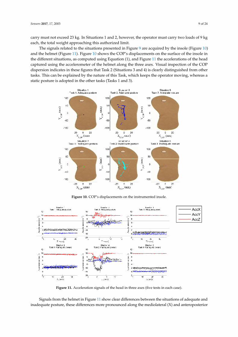
The signals related to the situations presented in Figure 9 are acquired by the insole (Figure 10) and the helmet (Figure 11). Figure 10 shows the COP’s displacements on the surface of the insole in the different situations, as computed using Equation (1), and Figure 11 the accelerations of the head captured using the accelerometer of the helmet along the three axes. Visual inspection of the COP

Figure 9. Six situations for evaluating adequate and inadequate posture for handling tasks, this figureis adapted from [53] with permission from Caroline Merola and the publisher.

Filling the distributors puts the operator in one of the situations represented in Figure 9. Some ofthese situations are inadequate, which means that they can lead to WMSDs in the long or mediumterm. Other positions are adequate, i.e., more secure for WMSD. We referred to Simoneau’s handlingmanual [53] to select the most frequent adequate and inadequate positions (as shown in Figure 9).

3.2. Experimental Protocol

A single participant wore both the helmet (Figure 2) and insole (Figure 3), and simulated twentytrials of each of the situations described in Figure 9. For Situations 1, 2, 5 and 6, to have a good reliabilityin the information delivered by the COP features while adopting a static position, the duration of themeasurement time must vary between 20 and 60 s. In our experiments, we set this duration to 20 s.For Situations 3 and 4, since there are movements, the duration was set to 15 s, i.e., the time needed toperform these movements. Each piece carried by the participant weighed 9 kg, a load considered asmoderately heavy. According to Canadian regulations [54], the maximum load that an operator must

Sensors 2017, 17, 2003 9 of 24

carry must not exceed 23 kg. In Situations 1 and 2, however, the operator must carry two loads of 9 kgeach, the total weight approaching this authorized limit.

The signals related to the situations presented in Figure 9 are acquired by the insole (Figure 10)and the helmet (Figure 11). Figure 10 shows the COP’s displacements on the surface of the insole inthe different situations, as computed using Equation (1), and Figure 11 the accelerations of the headcaptured using the accelerometer of the helmet along the three axes. Visual inspection of the COPdispersion indicates in these figures that Task 2 (Situations 3 and 4) is clearly distinguished from othertasks. This can be explained by the nature of this Task, which keeps the operator moving, whereas astatic posture is adopted in the other tasks (Tasks 1 and 3).

Sensors 2017, 17, 2003 9 of 24

dispersion indicates in these figures that Task 2 (Situations 3 and 4) is clearly distinguished from other tasks. This can be explained by the nature of this Task, which keeps the operator moving, whereas a static posture is adopted in the other tasks (Tasks 1 and 3).

Figure 10. COP’s displacements on the instrumented insole.

Figure 11. Acceleration signals of the head in three axes (five tests in each case).

Signals from the helmet in Figure 11 show clear differences between the situations of adequate and inadequate posture, these differences more pronounced along the mediolateral (X) and anteroposterior (Y) axes and when the operator is moving (Situations 3 and 4). This can also be seen Table 1, which gives the mean acceleration along axes X and Y for Situations 1, 2, 5 and 6. Moreover, in the case of static posture, the acceleration is nearly constant (the higher value observed for the Z axis is due to gravitation; Z axis is a perpendicular axis to insole surface). In contrast, head accelerations for Task 2 vary sharply due to the operator’s movements during this task.

Figure 10. COP’s displacements on the instrumented insole.

Sensors 2017, 17, 2003 9 of 24

dispersion indicates in these figures that Task 2 (Situations 3 and 4) is clearly distinguished from other tasks. This can be explained by the nature of this Task, which keeps the operator moving, whereas a static posture is adopted in the other tasks (Tasks 1 and 3).

Figure 10. COP’s displacements on the instrumented insole.

Figure 11. Acceleration signals of the head in three axes (five tests in each case).

Signals from the helmet in Figure 11 show clear differences between the situations of adequate and inadequate posture, these differences more pronounced along the mediolateral (X) and anteroposterior (Y) axes and when the operator is moving (Situations 3 and 4). This can also be seen Table 1, which gives the mean acceleration along axes X and Y for Situations 1, 2, 5 and 6. Moreover, in the case of static posture, the acceleration is nearly constant (the higher value observed for the Z axis is due to gravitation; Z axis is a perpendicular axis to insole surface). In contrast, head accelerations for Task 2 vary sharply due to the operator’s movements during this task.

Figure 11. Acceleration signals of the head in three axes (five tests in each case).

Signals from the helmet in Figure 11 show clear differences between the situations of adequate andinadequate posture, these differences more pronounced along the mediolateral (X) and anteroposterior

Sensors 2017, 17, 2003 10 of 24

(Y) axes and when the operator is moving (Situations 3 and 4). This can also be seen Table 1, which givesthe mean acceleration along axes X and Y for Situations 1, 2, 5 and 6. Moreover, in the case of staticposture, the acceleration is nearly constant (the higher value observed for the Z axis is due to gravitation;Z axis is a perpendicular axis to insole surface). In contrast, head accelerations for Task 2 vary sharplydue to the operator’s movements during this task.

Table 1. Approximation of the mean values of the head accelerations according the mediolateral (X)and the anteroposterior (Y).

Mean Value (ms−2) Situation 1 Situation 2 Situation 5 Situation 6

AccX ≈2 ≈2 ≈1 ≈2AccY ≈0 ≈2 ≈0 ≈0

Figures 10 and 11 present the recordings of a single trial and five trials respectively. To givea more complete view of the data, Figure 12 gives the areas (i.e., bounding boxes) containing theCOP displacements of all trials, recorded in each situation. We can note that for adequate postures(zones with black and red borders), the displacement zones are smaller, indicating a certain stabilitycompared to the inadequate static postures (zones with green and pink borders). This observationis not applicable when the operator is in motion (Situations 3 and 4). We can thus use the area ofdisplacement as a criterion to differentiate between specific postures. In this study, we considered thedisplacements along the mediolateral (Am_X) and anteroposterior (Am_Y) axes, as well as the ellipseof confidence surf_ellip (the area that keeps 90% of the points occupied by the COP).

Sensors 2017, 17, 2003 10 of 24

Table 1. Approximation of the mean values of the head accelerations according the mediolateral (X) and the anteroposterior (Y).

Mean Value (ms−2) Situation 1 Situation 2 Situation 5 Situation 6 AccX ≈2 ≈2 ≈1 ≈2 AccY ≈0 ≈2 ≈0 ≈0

Figures 10 and 11 present the recordings of a single trial and five trials respectively. To give a more complete view of the data, Figure 12 gives the areas (i.e., bounding boxes) containing the COP displacements of all trials, recorded in each situation. We can note that for adequate postures (zones with black and red borders), the displacement zones are smaller, indicating a certain stability compared to the inadequate static postures (zones with green and pink borders). This observation is not applicable when the operator is in motion (Situations 3 and 4). We can thus use the area of displacement as a criterion to differentiate between specific postures. In this study, we considered the displacements along the mediolateral (Am_X) and anteroposterior (Am_Y) axes, as well as the ellipse of confidence surf_ellip (the area that keeps 90% of the points occupied by the COP).

Figure 12. Areas containing the COP displacements measured in different situations.

4. Design of the Supervised Model for Posture Classification

The proposed approach for classifying postures is illustrated in Figure 13. It is composed of three distinct phases: (1) Data acquisition, where sample measurements are gathered through a set of sensors; (2) Data preprocessing, which includes features preparation and dimensionality reduction; and (3) Classification, in which the system uses the selected features to evaluate the incoming information and make a final decision as to which class this latter belongs.

Figure 13. The proposed approach for classifying postures, comprised of three phases: (1) data acquisition; (2) data preprocessing and (3) classification.

Figure 12. Areas containing the COP displacements measured in different situations.

4. Design of the Supervised Model for Posture Classification

The proposed approach for classifying postures is illustrated in Figure 13. It is composed of threedistinct phases: (1) Data acquisition, where sample measurements are gathered through a set of sensors;(2) Data preprocessing, which includes features preparation and dimensionality reduction; and (3)Classification, in which the system uses the selected features to evaluate the incoming information andmake a final decision as to which class this latter belongs.

Sensors 2017, 17, 2003 11 of 24

1

Figure 13. The proposed approach for classifying postures, comprised of three phases: (1) dataacquisition; (2) data preprocessing and (3) classification.

Data acquisition has already been presented in experimental protocol. The preprocessing andclassification phases are considered in the following sections.

4.1. Feature Preparation

In the processing phase, an initial set of features has to be computed. The goal of this phase is toextract discriminative features from the raw acquired data. Toward this goal, we used two differentapproaches, a direct approach and a graphic approach, which differ in the nature and the source ofextracted features.

4.1.1. The Direct Approach

In this approach, features are determined directly from the helmet and insole recordings.The features extracted from the head acceleration recordings along the three axes AccX, AccY andAccZ are mainly of statistical nature: mean values (i.e., AccXm, AccYm, AccZm), maximum values(i.e., AccXmax, AccYmax, AccZmax), variances (i.e., AccXvar, AccYvar, AccZvar), standard deviations(i.e., AccXstd, AccYstd, AccZstd), root mean squares (i.e., AccXrms, AccYrms, AccZrms), and kurtosis(i.e., AccXkurt, AccYkurt, AccZkurt).

Features extracted from COP recordings are based on two different representations:the statokinesigram (COP trajectory in the horizontal plane) and the stabilogram (variations of thetime series showing the anteroposterior YCOP and the mediolateral XCOP). Various features can beobtained from these representations to analyze the control postural while adopting a certain posture.Among these are global variables [36], which characterize the magnitude of XCOP, YCOP and their resultantin both time and frequency domains [55,56]. These variables are widely used in the literature for variousapplications, including postural control in aging (such as Parkinson’s and ataxia subjects) [55,57]. Featuresmay also be defined from structural variables, which describe the dynamic changes of postural swayby decomposing the COP sway patterns into subunits and correlating them with the motor controlprocess [55,56]. These variables are particularly useful to cover the non-stationary character of theCOP displacement. Examples of structural variables are those proposed by Collins and De Luca [58],which are based on the Stabilogram Diffusion Analysis method. This method models the trajectoryof the COP using stochastic processes such as the fractional Brownian motions. The Fractal Analysisdeveloped by Blaszczyk [59] also provides other structural variables related to postural perturbations.In the context of this work, we limited our selection of features to the set of global variables shownin Table 2. These features were grouped into three categories: spatiotemporal data extracted from thestatokinesigram, spatiotemporal data extracted from the stabilograms and frequency data.

Sensors 2017, 17, 2003 12 of 24

Table 2. List of the features extracted from the COP recordings (insole only).

Type Description Name

Spatiotemporal featuresextracted fromthe statokinesigram

The total length of the statokinesigram lg_tot

The mean and standard deviation of thestatokinesigram’s segments lengths m_lg_seg std_lg_seg

The distance between the first and last point ofthe statokinesigram dist_prdr

The amplitude of the displacement in themediolateral (XCOP) and anteroposterior (YCOP) axes Am_X Am_Y

The surface of the ellipse covering 90% of thedisplacements of the COP surf_ellip

The length/surface ratio, which informs us on theenergy spent by the subject during thepostural control

lfs

Spatiotemporal featuresextracted from thestabilograms

The mean and maximum values, the variances, thestandard deviations, the root-mean-squares and thekurtosis of the displacements in the mediolateral(XCOP) and anteroposterior (YCOP) axes.

Xm, Ym, Xmax, Ymax Xstd,Ystd, Xvar, Yvar Xrms,

Yrms, Xkurt, Ykurt

Statistical data related to the velocity (global,mediolateral and anteroposterior) such as mean andmaximum values, the variances, the standarddeviations, the root-mean-squares and the kurtosis

Vm, VXm, Vym Vmax,VXmax, Vymax Vstd,

VXstd, Vystd Vvar, Vxvar,Vyvar Vrms, VXrms, Vyrms

Vkurt, VXkurt, VYkurt

Frequential features Mean and median frequencies of the mediolateral(XCOP) and anteroposterior (YCOP) displacements

mnfreqX, mnfreqYmdfreqX, mdfreqY

4.1.2. The Graphic Approach

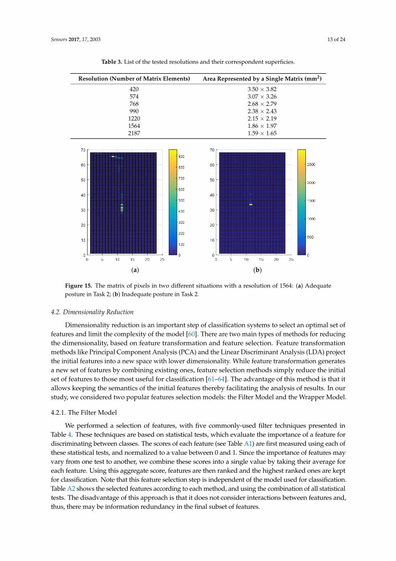
To acquire additional characteristics for differentiating between postural Situations, we alsoproposed a graphic approach which represents COP displacements from the insole as an image (matrixof pixels). To fix the surface of the insole to be discretized, we first computed the minimum/maximumvalues of XCOP and YCOP across all measurements. The resulting area, shown in Figure 14, has a totalsize of 43 × 134 mm2 and is discretized using different resolutions (i.e., number of pixels in the image).Table 3 gives the correspondence between the resolution and the corresponding area of a single matrixelement. The features obtained by this method are the elements of the matrix representing the area ofthe insole that has been occupied by the center of pressure at least once. Figure 15 shows an exampleof matrices obtained using this method.

Sensors 2017, 17, 2003 12 of 24

and De Luca [58], which are based on the Stabilogram Diffusion Analysis method. This method models the trajectory of the COP using stochastic processes such as the fractional Brownian motions. The Fractal Analysis developed by Blaszczyk [59] also provides other structural variables related to postural perturbations. In the context of this work, we limited our selection of features to the set of global variables shown in Table 2. These features were grouped into three categories: spatiotemporal data extracted from the statokinesigram, spatiotemporal data extracted from the stabilograms and frequency data.

4.1.2. The Graphic Approach

To acquire additional characteristics for differentiating between postural Situations, we also proposed a graphic approach which represents COP displacements from the insole as an image (matrix of pixels). To fix the surface of the insole to be discretized, we first computed the minimum/maximum values of XCOP and YCOP across all measurements. The resulting area, shown in Figure 14, has a total size of 43 × 134 mm2 and is discretized using different resolutions (i.e., number of pixels in the image). Table 3 gives the correspondence between the resolution and the corresponding area of a single matrix element. The features obtained by this method are the elements of the matrix representing the area of the insole that has been occupied by the center of pressure at least once. Figure 15 shows an example of matrices obtained using this method.

Figure 14. Representation of the area of the insole occupied by the COP.

(a) (b)

Figure 15. The matrix of pixels in two different situations with a resolution of 1564: (a) Adequate posture in Task 2; (b) Inadequate posture in Task 2.

Figure 14. Representation of the area of the insole occupied by the COP.

Sensors 2017, 17, 2003 13 of 24

Table 3. List of the tested resolutions and their correspondent superficies.

Resolution (Number of Matrix Elements) Area Represented by a Single Matrix (mm2)

420 3.50 × 3.82574 3.07 × 3.26768 2.68 × 2.79990 2.38 × 2.43

1220 2.15 × 2.191564 1.86 × 1.972187 1.59 × 1.65

Sensors 2017, 17, 2003 12 of 24

and De Luca [58], which are based on the Stabilogram Diffusion Analysis method. This method models the trajectory of the COP using stochastic processes such as the fractional Brownian motions. The Fractal Analysis developed by Blaszczyk [59] also provides other structural variables related to postural perturbations. In the context of this work, we limited our selection of features to the set of global variables shown in Table 2. These features were grouped into three categories: spatiotemporal data extracted from the statokinesigram, spatiotemporal data extracted from the stabilograms and frequency data.

4.1.2. The Graphic Approach

To acquire additional characteristics for differentiating between postural Situations, we also proposed a graphic approach which represents COP displacements from the insole as an image (matrix of pixels). To fix the surface of the insole to be discretized, we first computed the minimum/maximum values of XCOP and YCOP across all measurements. The resulting area, shown in Figure 14, has a total size of 43 × 134 mm2 and is discretized using different resolutions (i.e., number of pixels in the image). Table 3 gives the correspondence between the resolution and the corresponding area of a single matrix element. The features obtained by this method are the elements of the matrix representing the area of the insole that has been occupied by the center of pressure at least once. Figure 15 shows an example of matrices obtained using this method.

Figure 14. Representation of the area of the insole occupied by the COP.

(a) (b)

Figure 15. The matrix of pixels in two different situations with a resolution of 1564: (a) Adequate posture in Task 2; (b) Inadequate posture in Task 2. Figure 15. The matrix of pixels in two different situations with a resolution of 1564: (a) Adequateposture in Task 2; (b) Inadequate posture in Task 2.

4.2. Dimensionality Reduction

Dimensionality reduction is an important step of classification systems to select an optimal set offeatures and limit the complexity of the model [60]. There are two main types of methods for reducingthe dimensionality, based on feature transformation and feature selection. Feature transformationmethods like Principal Component Analysis (PCA) and the Linear Discriminant Analysis (LDA) projectthe initial features into a new space with lower dimensionality. While feature transformation generatesa new set of features by combining existing ones, feature selection methods simply reduce the initialset of features to those most useful for classification [61–64]. The advantage of this method is that itallows keeping the semantics of the initial features thereby facilitating the analysis of results. In ourstudy, we considered two popular features selection models: the Filter Model and the Wrapper Model.

4.2.1. The Filter Model

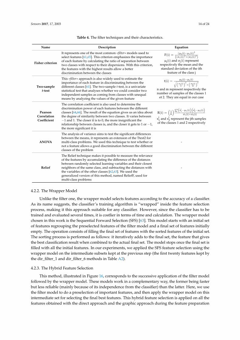
We performed a selection of features, with five commonly-used filter techniques presented inTable 4. These techniques are based on statistical tests, which evaluate the importance of a feature fordiscriminating between classes. The scores of each feature (see Table A1) are first measured using each ofthese statistical tests, and normalized to a value between 0 and 1. Since the importance of features mayvary from one test to another, we combine these scores into a single value by taking their average foreach feature. Using this aggregate score, features are then ranked and the highest ranked ones are keptfor classification. Note that this feature selection step is independent of the model used for classification.Table A2 shows the selected features according to each method, and using the combination of all statisticaltests. The disadvantage of this approach is that it does not consider interactions between features and,thus, there may be information redundancy in the final subset of features.

Sensors 2017, 17, 2003 14 of 24

Table 4. The filter techniques and their characteristics.

Name Description Equation

Fisher criterion

It represents one of the most common «filter» models used toselect features [61,65]. This criterion emphasizes the importanceof each feature by calculating the ratio of separation betweentwo classes with respect to their dispersions. With this criterion,the features with the highest results allow a betterdiscrimination between the classes

F(i) = (µ2(i)−µ1(i))2

((σ1(i))2+(σ2(i))

2)µj(i) and σj(i) represent

respectively the mean and thestandard deviation of the ith

feature of the class j

Two-samplet-test

This «filter» approach is also widely used to estimate theimportance of each feature in discriminating between thedifferent classes [61]. The two-sample t-test, is a univariatestatistical test that analyses whether we could consider twoindependent samples as coming from classes with unequalmeans by analyzing the values of the given feature

t(i) = µ2(i)−µ1(i)√(σ1(i)

n

)2+(

σ2(i)m

)2

n and m represent respectively thenumber of samples of the classes 1

et 2. They are equal in our case

PearsonCorrelationCoefficient

The correlation coefficient is also used to determine thediscrimination power of each features between the differentclasses [64,66]. The result of the equation gives us an idea aboutthe degree of similarity between two classes. It varies between−1 and 1. The closer it is to 0, the more insignificant therelationship between classes is, and the closer it gets to 1 or −1,the more significant it is

R(i) =(

1n

)∑nj

(xj

1−µ1(i))(

xj2−µ2(i)

)σ1(i)×σ2(i)

xj1 and xj

2 represent the jth samplesof the classes 1 and 2 respectively

ANOVA

The analysis of variance aims to test the significant differencesbetween the means, it represents an extension of the Ttest2 formulti-class problems. We used this technique to test whether ornot a feature allows a good discrimination between the differentclasses of the problem

-

Relief

The Relief technique makes it possible to measure the relevanceof the features by accumulating the difference of the distancesbetween randomly selected learning variables and their closestneighbors of the same class, and subtracting the distances withthe variables of the other classes [62,63]. We used thegeneralized version of this method, named ReliefF, used formulti-class problems

-

4.2.2. The Wrapper Model

Unlike the filter one, the wrapper model selects features according to the accuracy of a classifier.As its name suggests, the classifier’s training algorithm is “wrapped” inside the feature selectionprocess, making it this approach suitable for any classifier. However, since the classifier has to betrained and evaluated several times, it is costlier in terms of time and calculation. The wrapper modelchosen in this work is the Sequential Forward Selection (SFS) [63]. This model starts with an initial setof features regrouping the preselected features of the filter model and a final set of features initiallyempty. The operation consists of filling the final set of features with the sorted features of the initial set.The sorting process is performed as follows: it iteratively adds to the final set, the feature that givesthe best classification result when combined to the actual final set. The model stops once the final set isfilled with all the initial features. In our experiments, we applied the SFS feature selection using thewrapper model on the intermediate subsets kept at the previous step (the first twenty features kept bythe dir_filter_1 and dir_filter_6 methods in Table A2).

4.2.3. The Hybrid Feature Selection

This method, illustrated in Figure 16, corresponds to the successive application of the filter modelfollowed by the wrapper model. These models work in a complementary way, the former being fasterbut less reliable (mainly because of its independence from the classifier) than the latter. Here, we usethe filter model to do a preselection of important features, and then apply the wrapper model on thisintermediate set for selecting the final best features. This hybrid feature selection is applied on all thefeatures obtained with the direct approach and the graphic approach during the feature preparation

Sensors 2017, 17, 2003 15 of 24

process. Using the hybrid feature selection method, the 60 direct approach features (Table A1) havebeen reduced to eight (Table 5) and the 990 graphic approach features to three.

Sensors 2017, 17, 2003 15 of 24

Figure 16. The hybrid model for feature selection.

Table 5. List of the best «Direct» features obtained with the method dir_hybride_1 (dir_filter_1 (Test2) and wrapper).

Id Name Description Tool 55 AccZm Mean acceleration of the head along the axis Z Helmet 10 Yvar YCOP variance Insole 51 AccYstd Standard deviation of the acceleration along the axis Y Helmet 47 AccXrms The root mean square of the acceleration along the axis X Helmet 3 Xstd Standard deviation of XCOP Insole 49 AccYm Mean acceleration of the head along the axis Y Helmet 44 AccXmax Maximal head acceleration along the axis X Helmet 52 AccYvar Variance of the head acceleration along the axis Y Helmet

4.3. Classification Phase

After feature selection, we proceeded with the classification process. Given the recent successes of Artificial Neural Networks (ANN), in this work, we chose a multi-layer perceptron as classifier. Our network is organized as follows:

An input layer of i neurons, where i is the number of inputs (i.e., final set features); A hidden layer of j = 12 neurons whose activation function is the hyperbolic tangent; An output layer of k = 6 neurons, where k is the number of classes (posture situations presented

previously). A softmax function is used to convert the output of these neurons into class probabilities [67].

As in most classification networks [68,69], cross-entropy is used as loss function:

E = 1l T ln S (2)

where k represents the number of classes, l represents the total number of sample groups and Tij is the desired response of the output neuron i of the sample group j. The specificity of this function is that it strongly penalizes the wrong outputs (whose values are far from the desired value Tij and thus closer to (1−Tij)) and emphasize those that are correct [69]. As a learning algorithm, we adopted the conjugate gradient method. This method is appropriate for classification problems when the volume of data is not very large [68].

Figure 16. The hybrid model for feature selection.

Table 5. List of the best «Direct» features obtained with the method dir_hybride_1 (dir_filter_1 (Test2)and wrapper).

Id Name Description Tool

55 AccZm Mean acceleration of the head along the axis Z Helmet10 Yvar YCOP variance Insole51 AccYstd Standard deviation of the acceleration along the axis Y Helmet47 AccXrms The root mean square of the acceleration along the axis X Helmet3 Xstd Standard deviation of XCOP Insole49 AccYm Mean acceleration of the head along the axis Y Helmet44 AccXmax Maximal head acceleration along the axis X Helmet52 AccYvar Variance of the head acceleration along the axis Y Helmet

4.3. Classification Phase

After feature selection, we proceeded with the classification process. Given the recent successesof Artificial Neural Networks (ANN), in this work, we chose a multi-layer perceptron as classifier.Our network is organized as follows:

• An input layer of i neurons, where i is the number of inputs (i.e., final set features);• A hidden layer of j = 12 neurons whose activation function is the hyperbolic tangent;• An output layer of k = 6 neurons, where k is the number of classes (posture situations presented

previously). A softmax function is used to convert the output of these neurons into classprobabilities [67].

As in most classification networks [68,69], cross-entropy is used as loss function:

E =1l

l

∑j=1

k

∑n=1

Tij ln(Sij)

(2)

where k represents the number of classes, l represents the total number of sample groups and Tij isthe desired response of the output neuron i of the sample group j. The specificity of this function isthat it strongly penalizes the wrong outputs (whose values are far from the desired value Tij and thuscloser to (1−Tij)) and emphasize those that are correct [69]. As a learning algorithm, we adopted the

Sensors 2017, 17, 2003 16 of 24

conjugate gradient method. This method is appropriate for classification problems when the volumeof data is not very large [68].

5. Classification Results and Discussion

Bestaven et al. [70] show that the total center of pressure (TCOP) displacements, initially locatedbetween the two feet, seems to be a good tool to identify some strategies but during the sit-to-walkespecially in the elderly. Several studies cited in [42,43] have shown that COP does not differ betweendominant and non-dominant limbs. Thereby, in our study, we therefore believe that no effect canbe observed on the results of measurement by both feet. The goal of this study is to use a minimalconfiguration and architecture allowing the classification of six postures in order to develop aninexpensive assistance device which can be used at work in real environment. This system is mainlydesigned for a long-term monitoring of worker. Then, using one insole is an efficient solution givingan adequate classification of postures presented below:

5.1. Application of the Filter Technique on the Direct Approach Features

In Table A2, we notice that most of the tests kept more or less the same features in their topten lists, which allowed us to keep the overall score naturally. The only exception is the Pearsontest (dir_filter_2 method), which gave one of the poorest classification performances. We tested thedifferent sets of features on a neural network, using a 10-fold cross validation technique. For morereliable results, this cross-validation process was repeated 10 times, and the average classification rateover these 10 runs used as final performance measure.

Figure 17 shows the mean classification rate of the feature selection techniques, for different numbersof selected features. We notice a poor performance when no feature selection is used. For most featureselection methods, classification rates reach a peak performance (around 80%) between 20 and 30 features,this performance remaining stable for larger numbers of feature. To have an efficient classifier, we limitthe number of features to 20. Using this limit, Ttest2 (dir_filter_1 method) gave the best classificationresult, followed by the combination of all the scores (dir_filter_6 method). Therefore, we kept the first20 features of these two methods as intermediate subsets of features for the wrapper technique.

Sensors 2017, 17, 2003 16 of 24

5. Classification Results and Discussion

Bestaven et al. [70] show that the total center of pressure (TCOP) displacements, initially located between the two feet, seems to be a good tool to identify some strategies but during the sit-to-walk especially in the elderly. Several studies cited in [42,43] have shown that COP does not differ between dominant and non-dominant limbs. Thereby, in our study, we therefore believe that no effect can be observed on the results of measurement by both feet. The goal of this study is to use a minimal configuration and architecture allowing the classification of six postures in order to develop an inexpensive assistance device which can be used at work in real environment. This system is mainly designed for a long-term monitoring of worker. Then, using one insole is an efficient solution giving an adequate classification of postures presented below:

5.1. Application of the Filter Technique on the Direct Approach Features

In Table A2, we notice that most of the tests kept more or less the same features in their top ten lists, which allowed us to keep the overall score naturally. The only exception is the Pearson test (dir_filter_2 method), which gave one of the poorest classification performances. We tested the different sets of features on a neural network, using a 10-fold cross validation technique. For more reliable results, this cross-validation process was repeated 10 times, and the average classification rate over these 10 runs used as final performance measure.

Figure 17 shows the mean classification rate of the feature selection techniques, for different numbers of selected features. We notice a poor performance when no feature selection is used. For most feature selection methods, classification rates reach a peak performance (around 80%) between 20 and 30 features, this performance remaining stable for larger numbers of feature. To have an efficient classifier, we limit the number of features to 20. Using this limit, Ttest2 (dir_filter_1 method) gave the best classification result, followed by the combination of all the scores (dir_filter_6 method). Therefore, we kept the first 20 features of these two methods as intermediate subsets of features for the wrapper technique.

Figure 17. Averages of the recognition rates obtained by the filter selection method.

5.2. Application of the Hybrid Feature Selection on the Direct Approach Features

Table A3 gives the importance-sorted list of features obtained with the dir_hybride_1 and dir_hybride_2 methods (i.e., dir_filter_1 and dir_filter_6 technique, respectively, followed by the SFS wrapper). The classification results of these two methods are shown in Figure 18. To compare the

Figure 17. Averages of the recognition rates obtained by the filter selection method.

5.2. Application of the Hybrid Feature Selection on the Direct Approach Features

Table A3 gives the importance-sorted list of features obtained with the dir_hybride_1 anddir_hybride_2 methods (i.e., dir_filter_1 and dir_filter_6 technique, respectively, followed by the

Sensors 2017, 17, 2003 17 of 24

SFS wrapper). The classification results of these two methods are shown in Figure 18. To compare thehybrid feature selection method with using the filter method alone, and highlight the contribution ofthe wrapper model, the figure also gives the network’s performance corresponding to the features keptby dir_filter_1 and dir_filter_6. For both these filter models, we notice an increase in performance whengoing from the filter alone to the hybrid model. Comparing the two hybrid methods, no significantdifference in performance can be seen. Overall, a best performance of 90% was obtained by thedir_hybride_1 method using only eight features.

Sensors 2017, 17, 2003 17 of 24

hybrid feature selection method with using the filter method alone, and highlight the contribution of the wrapper model, the figure also gives the network’s performance corresponding to the features kept by dir_filter_1 and dir_filter_6. For both these filter models, we notice an increase in performance when going from the filter alone to the hybrid model. Comparing the two hybrid methods, no significant difference in performance can be seen. Overall, a best performance of 90% was obtained by the dir_hybride_1 method using only eight features.

Figure 18. Comparison between the performances of the filter and the hybrid selection methods.

5.3. Application of the Hybrid Feature Selection on the Graphic Approach Features

We applied dir_hybride_1 and dir_hybride_2 (described in Table A3) to the graphic approach features, the resulting methods called graph_hybride_1 and graph_hybride_2, respectively. Since both these methods selected the same features (with similar feature rankings), we only show in Figure 19. the classification results of graph_hybride_2. These results indicate that using the graphic approach features alone leads to poor performances, with a best classification rate near 60% (matrix resolution of 990). In the next section, we improve our results by combining these features with those of the direct approach.

Figure 19. Performance of the neural network with the graphical method according to different resolutions.

Number of Features1 1.5 2 2.5 3 3.5 4 4.5 5 5.5 6

0

0.1

0.2

0.3

0.4

0.5

0.6

0.7

0.8

0.9

1graph_hybrid_2 method with a resolution of 420graph_hybrid_2 method with a resolution of 574graph_hybrid_2 method with a resolution of 768graph_hybrid_2 method with a resolution of 990graph_hybrid_2 method with a resolution of 1220graph_hybrid_2 method with a resolution of 1564graph_hybrid_2 method with a resolution of 2187

Figure 18. Comparison between the performances of the filter and the hybrid selection methods.

5.3. Application of the Hybrid Feature Selection on the Graphic Approach Features

We applied dir_hybride_1 and dir_hybride_2 (described in Table A3) to the graphic approachfeatures, the resulting methods called graph_hybride_1 and graph_hybride_2, respectively. Since boththese methods selected the same features (with similar feature rankings), we only show in Figure 19.the classification results of graph_hybride_2. These results indicate that using the graphic approachfeatures alone leads to poor performances, with a best classification rate near 60% (matrix resolutionof 990). In the next section, we improve our results by combining these features with those of thedirect approach.

Sensors 2017, 17, 2003 17 of 24

hybrid feature selection method with using the filter method alone, and highlight the contribution of the wrapper model, the figure also gives the network’s performance corresponding to the features kept by dir_filter_1 and dir_filter_6. For both these filter models, we notice an increase in performance when going from the filter alone to the hybrid model. Comparing the two hybrid methods, no significant difference in performance can be seen. Overall, a best performance of 90% was obtained by the dir_hybride_1 method using only eight features.

Figure 18. Comparison between the performances of the filter and the hybrid selection methods.

5.3. Application of the Hybrid Feature Selection on the Graphic Approach Features

We applied dir_hybride_1 and dir_hybride_2 (described in Table A3) to the graphic approach features, the resulting methods called graph_hybride_1 and graph_hybride_2, respectively. Since both these methods selected the same features (with similar feature rankings), we only show in Figure 19. the classification results of graph_hybride_2. These results indicate that using the graphic approach features alone leads to poor performances, with a best classification rate near 60% (matrix resolution of 990). In the next section, we improve our results by combining these features with those of the direct approach.

Figure 19. Performance of the neural network with the graphical method according to different resolutions.

Number of Features1 1.5 2 2.5 3 3.5 4 4.5 5 5.5 6

0

0.1

0.2

0.3

0.4

0.5

0.6

0.7

0.8

0.9

1graph_hybrid_2 method with a resolution of 420graph_hybrid_2 method with a resolution of 574graph_hybrid_2 method with a resolution of 768graph_hybrid_2 method with a resolution of 990graph_hybrid_2 method with a resolution of 1220graph_hybrid_2 method with a resolution of 1564graph_hybrid_2 method with a resolution of 2187

Figure 19. Performance of the neural network with the graphical method according to different resolutions.

Sensors 2017, 17, 2003 18 of 24

5.4. Combination of Direct and Graph Approach Features

We added the three best features of the graphic approach, obtained by applying thegraph_hybride_1 method, to the features of the direct approach selected via the dir_hybride_1 anddir_hybride_2 methods (shown previously in Figure 18). We name integrate_1 and integrate_2,respectively, these two combinations of features. The classification results of these methods are shownin Figure 20. It can be seen that combining features improves results, the classification rate nowreaching 95% when using the eight best features (presented by order of importance in Table 5) ofdir_hybride_1 with the three best features of graph_hybride_1. We note that this result is achievedwith only 11 features from the initial set of 1050 features.

Sensors 2017, 17, 2003 18 of 24

5.4. Combination of Direct and Graph Approach Features

We added the three best features of the graphic approach, obtained by applying the graph_hybride_1 method, to the features of the direct approach selected via the dir_hybride_1 and dir_hybride_2 methods (shown previously in Figure 18). We name integrate_1 and integrate_2, respectively, these two combinations of features. The classification results of these methods are shown in Figure 20. It can be seen that combining features improves results, the classification rate now reaching 95% when using the eight best features (presented by order of importance in Table 5) of dir_hybride_1 with the three best features of graph_hybride_1. We note that this result is achieved with only 11 features from the initial set of 1050 features.

Figure 20. The integration of the direct and graphical methods.

6. Conclusions and Future Works

This study aimed to design an automated assessment tool for posture analysis. Using specific features, we demonstrated that artificial neural networks (ANN) can effectively be used to detect inadequate postures of individuals in a work environment. A direct approach was used to collect features from different postures and movements. We also introduced an innovative graphic approach, which represents movements of the center of pressure, captured by the insole, as an image. A hybrid model was used to select the most discriminative features generated by these two approaches. An important contribution of this study was to combine features from both approaches for the effective identification and prevention of inadequate postures. The proposed methodology allowed us to improve the recognition rate from 90% to 95%, an accuracy superior to that of existing models.

A limitation of this study is the small sample size, which was obtained using a single participant. Although our results suggest that the proposed method can be used successfully to assess work-related MSDs, testing on a larger dataset with multiple participants would help to further validate these results. Future research can also apply the Graphic approach to extract features from the helmet recordings. Toward this goal, measurements of the IMU can be exploited to determine the trajectories of the head in the planes formed by its three axes of motion, namely the plane (X, Y), the plane (Y, Z) and the plane (X, Z). Subsequently, as with COP displacements, we can use three matrices representing these trajectories. We also plan to integrate other inertial units located in areas of the body, such as the back and the upper/lower limbs. Adding these new sensors in other locations may improve the accuracy of the system. In addition, these sensors (specifically those in the upper limbs) may detect repetitive movements, which are one of the major risk factors aside from awkward postures and movements. Finally, we can extend our detection system to significant muscle efforts, for instance, detected via an electromyogram (EMG).

Figure 20. The integration of the direct and graphical methods.

6. Conclusions and Future Works

This study aimed to design an automated assessment tool for posture analysis. Using specificfeatures, we demonstrated that artificial neural networks (ANN) can effectively be used to detectinadequate postures of individuals in a work environment. A direct approach was used to collectfeatures from different postures and movements. We also introduced an innovative graphic approach,which represents movements of the center of pressure, captured by the insole, as an image. A hybridmodel was used to select the most discriminative features generated by these two approaches.An important contribution of this study was to combine features from both approaches for theeffective identification and prevention of inadequate postures. The proposed methodology allowed usto improve the recognition rate from 90% to 95%, an accuracy superior to that of existing models.

A limitation of this study is the small sample size, which was obtained using a single participant.Although our results suggest that the proposed method can be used successfully to assess work-relatedMSDs, testing on a larger dataset with multiple participants would help to further validate these results.Future research can also apply the Graphic approach to extract features from the helmet recordings.Toward this goal, measurements of the IMU can be exploited to determine the trajectories of the headin the planes formed by its three axes of motion, namely the plane (X, Y), the plane (Y, Z) and theplane (X, Z). Subsequently, as with COP displacements, we can use three matrices representing thesetrajectories. We also plan to integrate other inertial units located in areas of the body, such as the backand the upper/lower limbs. Adding these new sensors in other locations may improve the accuracyof the system. In addition, these sensors (specifically those in the upper limbs) may detect repetitivemovements, which are one of the major risk factors aside from awkward postures and movements.

Sensors 2017, 17, 2003 19 of 24

Finally, we can extend our detection system to significant muscle efforts, for instance, detected via anelectromyogram (EMG).

Acknowledgments: This work is supported by the financial support of the Fonds de recherche du Québec—Natureet technologies (FRQNT), under the grant number 2016-PR-188869. We would like to thank Automation and 3DMultimodal Intelligent Interaction (LAIMI) Laboratory at University of Quebec at Chicoutimi (UQAC).

Author Contributions: Eya Barkallah and Johan Freulard conceived, designed the experiments; performedthe experiments and analyzed the data; Martin J-.D. Otis (research director of Johan Freulard) contributedreagents/materials/analysis tools and designed the insole and helmet; Eya Barkallah, Johan Freulard andJohannes C. Ayena wrote the paper. Suzy Ngomo (co-director of Eya Barkallah) designed the experiments andvalidate the scientific contents; Christian Desrosiers, as a director of Johannes C. Ayena, validate the scientificcontents. Martin J-.D. Otis, Suzy Ngomo and Christian Desrosiers have been involved in drafting the manuscriptand revising it critically so that it is important content. Martin J-.D. Otis, Suzy Ngomo and Christian Desrosiersare holding the grant from FRQ-NT.

Conflicts of Interest: The authors declare no conflict of interest. The founding organization (FRQ-NT) had no rolein the design of the study; in the collection, analyses, or interpretation of data; in the writing of the manuscript,and in the decision to publish the results.

Appendix A

Table A1. Scores obtained by the filter feature selection methods.

Id Name Anova(p-Value)

Ttest2(p-Value)

Pearson(Score) Fisher (Score) Relief (Score) Final

(Score)

1 Xm 8.43 × 10−32 1.06 × 10-1 2.64 × 10−2 2.63 1.84 × 10−1 0.4432 Xmax 3.55 × 10−24 1.10 × 10−1 −6.51 × 10−2 1.90 2.97 × 10−1 0.3383 Xstd 3.88 × 10−54 3.53 × 10−2 −5.27 × 10−2 7.01 2.79 × 10−1 0.3244 Xvar 6.28 × 10−40 1.30 × 10−1 −4.98 × 10−2 3.97 2.04 × 10−1 0.3945 Xrms 8.03 × 10−29 9.36 × 10−2 −5.45 × 10−2 2.06 1.61 × 10−1 0.3996 Xkurt 5.05 × 10−1 2.28 × 10−1 −4.26 × 10−2 6.28 × 10−1 6.22 × 10−3 0.6257 Ym 1.16 × 10−57 2.47 × 10−2 −6.02 × 10−2 11.20 2.38 × 10−1 0.3318 Ymax 1.03 × 10−75 1.46 × 10−1 2.10 × 10−2 2.83 × 102 4.56 × 10−1 0.1359 Ystd 2.21 × 10−93 2.64 × 10−3 5.44 × 10−2 40.5 3.34 × 10−1 0.33010 Yvar 1.08 × 10−66 2.18 × 10−2 9.64 × 10−3 11.10 2.23 × 10−1 0.37911 Yrms 1.09 × 10−69 1.82 × 10−2 7.27 × 10−32 10.90 2.32 × 10−1 0.41312 Ykurt 4.06 × 10−1 2.89 × 10−1 2.11 × 10−1 3.79 × 10−1 4.13x10−3 0.78413 Vm 1.45 × 10−48 1.22 × 10−1 5.01 × 10−4 5.52 2.41 × 10−1 0.40514 Vmax 1.04 × 10−19 1.69 × 10−1 4.47 × 10−2 2.91 9.14 × 10−2 0.51715 Vstd 4.16 × 10−34 1.79 × 10−1 −8.17 × 10−3 3.08 1.52 × 10−1 0.46016 Vvar 9.64 × 10−35 1.50 × 10−1 5.97 × 10−3 3.19 1.55 × 10−1 0.45717 Vrms 4.33x10−11 1.87 × 10−1 −7.68 × 10−3 8.34 × 10−1 4.84 × 10−2 0.51118 Vkurt 4.50x10−5 2.10 × 10−1 4.93 × 10−2 3.72 × 10−1 4.52 × 10−2 0.55619 VXm 9.86 × 10−1 5.00 × 10−1 3.55 × 10−2 3.59 × 10−2 4.98 × 10−3 0.86720 VXmax 1.60 × 10−17 2.16 × 10−1 3.50 × 10−2 2.41 6.11 × 10−2 0.54121 VXstd 2.74 × 10−31 2.22 × 10−1 −2.70 × 10−2 2.89 1.07 × 10−1 0.48422 VXvar 2.78 × 10−31 2.22 × 10−1 −2.70 × 10−2 2.89 1.07 × 10−1 0.48423 VXrms 2.51 × 10−9 2.46 × 10−1 −1.08 × 10−2 8.32 × 10−1 2.26 × 10−2 0.54124 VXkurt 1.72 × 10−9 2.28 × 10−1 −1.52 × 10−2 6.61 × 10−1 6.78 × 10−2 0.51225 Vym 9.76 × 10−1 5.70 × 10−1 6.22 × 10−3 2.76 × 10−2 7.69 × 10−3 0.87126 VYmax 3.30 × 10−15 1.94 × 10−1 2.56 × 10−2 1.14 5.99 × 10−2 0.52927 VYstd 2.48 × 10−31 1.59 × 10−1 1.28 × 10−2 2.50 1.45 × 10−1 0.47028 VYvar 2.52 × 10−31 1.59 × 10−1 1.29 × 10−2 2.50 1.45 × 10−1 0.47029 VYrms 2.13 × 10−9 1.58 × 10−1 1.52 × 10−2 7.00 × 10−1 4.49 × 10−2 0.51730 VYkurt 1.12 × 10−7 1.81 × 10−1 4.79 × 10−2 5.48 × 10−1 6.13 × 10−2 0.53831 long_tot 1.54 × 10−45 9.67 × 10−2 4.98 × 10−3 4.42 1.92 × 10−1 0.42132 m_long_seg 6.90 × 10−50 1.03 × 10−1 6.50 × 10−3 5.51 2.33 × 10−1 0.40533 std_long_seg 2.78 × 10−44 1.26 × 10−1 2.96 × 10−2 4.19 2.10 × 10−1 0.43934 dist_prdr 2.39 × 10−2 1.55 × 10−1 4.08 × 10−2 2.62 × 10−1 7.15 × 10−3 0.553

Sensors 2017, 17, 2003 20 of 24

Table A1. Cont.

Id Name Anova(p-Value)

Ttest2(p-Value)

Pearson(Score) Fisher (Score) Relief (Score) Final

(Score)

35 plage_X 1.79 × 10−53 7.59 × 10−2 −4.99 × 10−2 7.52 3.88 × 10−1 0.29136 plage_Y 2.14 × 10−59 9.94 × 10−2 2.05 × 10−1 12.10 3.28 × 10−1 0.48037 surf_ellip 5.65 × 10−49 4.67 × 10−2 −3.49 × 10−2 5.40 2.36 × 10−1 0.35938 Lfs 8.33 × 10−9 2.40 × 10−2 6.83 × 10−2 6.18 × 10−1 3.39 × 10−2 0.50739 mnfreqX 4.08 × 10−29 1.47 × 10−1 −2.06 × 10−2 2.06 1.40 × 10−1 0.44840 mnfreqY 9.05 × 10−31 7.43 × 10−2 1.45 × 10−1 2.88 1.37 × 10−1 0.52541 mdfreqX 7.60 × 10−29 7.92 × 10−2 9.55 × 10−3 2.19 1.27 × 10−1 0.44842 mdfreqY 4.83 × 10−31 3.74 × 10−2 1.31 × 10−1 2.83 1.19 × 10−1 0.51143 AccXm 2.19 × 10−40 7.51 × 10−2 1.62 × 10−1 6.33 2.05 × 10−1 0.50344 AccXmax 1.94 × 10−34 7.24 × 10−2 8.73 × 10−2 4.36 1.94 × 10−1 0.46245 AccXstd 2.21 × 10−95 6.56 × 10−2 −1.89 × 10−2 66.30 3.24 × 10−1 0.29346 AccXvar 2.77 × 10−60 9.76 × 10−2 6.33 × 10−2 2.16 × 101 2.33 × 10−1 0.42747 AccXrms 1.12 × 10−87 5.78 × 10−2 −4.74 × 10−2 2.01 × 101 2.55 × 10−1 0.33648 AccXkurt 7.37 × 10−2 3.33 × 10−1 1.73 × 10−2 1.55 × 10−1 8.31 × 10−3 0.61149 AccYm 1.74 × 10−42 8.42 × 10−4 −2.31 × 10−2 6.46 2.02 × 10−1 0.36450 AccYmax 5.61 × 10−31 9.43 × 10−3 −9.55 × 10−2 4.48 1.47 × 10−1 0.34951 AccYstd 3.04 × 10−72 3.26 × 10−4 −3.65 × 10−2 17.80 3.34 × 10−1 0.28952 AccYvar 4.14 × 10−48 3.44 × 10−2 −7.64 × 10−5 9.98 2.23 × 10−1 0.37953 AccYrms 6.35 × 10−54 1.46 × 10−3 −3.38 × 10−2 6.62 2.66 × 10−1 0.33054 AccYkurt 5.93 × 10−1 3.47 × 10−1 −1.15 × 10−1 1.86 × 10−1 6.84 × 10−3 0.64155 AccZm 1.15 × 10−66 3.23 × 10−2 5.87 × 10−3 1.55 × 101 3.14 × 10−1 0.33756 AccZmax 7.20 × 10−32 1.06 × 10−1 8.16 × 10−2 8.62 1.86 × 10−1 0.47157 AccZstd 1.45 × 10−72 2.44 × 10−3 −8.06 × 10−2 19.90 3.18 × 10−1 0.26858 AccZvar 1.29 × 10−70 1.06 × 10−3 5.93 × 10−2 18.00 2.61 × 10−1 0.38159 AccZrms 7.42 × 10−53 2.66 × 10−3 −6.87 × 10−2 6.41 2.19 × 10−1 0.33060 AccZkurt 7.72 × 10−8 3.32 × 10−1 1.18 × 10−1 6.57 × 10−1 6.09 × 10−2 0.634

Table A2. Features kept by the filter feature selection methods.

Method Features Kept (from the Most Relevant to the Least))Name Test

dir_filter_1 Ttest 2 (p-value ≥ 0.05) 51-49-58-53-57-9-59-50-11-10-38-7-55-52-3-42-37

dir_filter_2 Pearson52-13-31-55-16-25-32-17-15-41-10-23-27-28-29-24-48-45-39-8-49-26-1-21-22-33-53-37-20-19-51-34-6-14-47-30-18-4-35-3-9-5-58-7-46-2-38-59-11-57-56-44-50-54-60-42-40-43-36-12

dir_filter_3 Fisher8-45-9-46-47-57-58-51-55-36-7-10-11-52-56-35-3-53-49-59-43-13-32-37-50-31-44-33-4-16-15-14-21-22-40-42-1-27-28-20-41-5-39-2-26-17-23-29-24-60-6-38-30-12-18-34-54-48-19-25

dir_filter_4 Anova (p-value ≥ 0.05)45-9-47-8-57-51-58-11-10-55-46-36-7-3-53-35-59-32-37-13-52-31-33-49-43-4-16-44-15-56-1-27-28-21-22-42-50-40-39-41-5-2-14-20-26-17-24-29-23-38-60-30-18-34-48

dir_filter_5 Relief8-35-51-9-36-45-57-55-2-3-53-58-47-13-7-37-32-46-11-10-52-59-33-43-4-49-44-31-56-1-5-16-15-50-27-28-39-40-41-42-21-22-14-24-30-20-60-26-17-18-29-38-23-48-25-34-54-6-19-12

dir_filter_6 Combination (combination of all tests)8-57-51-35-45-3-59-53-9-7-47-55-2-50-37-49-52-10-58-4-5-13-32-11-31-46-33-1-39-41-16-15-44-27-28-56-36-21-22-43-38-42-17-24-14-29-40-26-30-20-23-34-18-48-6-60-54-12-19-25

Table A3. Features kept with the hybrid feature selection methods.

Name Description Features Kept (from the Most Relevant to the Least)

dir_hybride_1 dir_filter_1 (Ttest2) + wrapper (SFS) 55-10-51-47-3-49-44-52-9-45-59-42-53-37-7-57-58-50-38-11

dir_hybride_2 dir_filter_6 (Combination) + wrapper (SFS) 10-49-58-7-9-37-51-45-52-3-31-53-59-55-13-32-57-35-47-8

Sensors 2017, 17, 2003 21 of 24

References

1. Da Costa, B.R.; Vieira, E.R. Risk factors for work-related musculoskeletal disorders: A systematic review ofrecent longitudinal studies. Am. J. Ind. Med. 2010, 53, 285–323. [CrossRef] [PubMed]

2. Roy, J.S.; Moffet, H.; McFadyen, B.J. Upper limb motor strategies in persons with and without shoulderimpingement syndrome across different speeds of movement. Clin. Biomech. 2008, 23, 1227–1236. [CrossRef][PubMed]

3. MacDermid, J.C.; Ramos, J.; Drosdowech, D.; Faber, K.; Patterson, S. The impact of rotator cuff pathologyon isometric and isokinetic strength, function, and quality of life. J. Shoulder Elb. Surg. 2004, 13, 593–598.[CrossRef]

4. Badley, E.M.; Rasooly, I.; Webster, G.K. Relative importance of musculoskeletal disorders as a cause ofchronic health problems, disability, and health care utilization: Findings from the 1990 ontario health survey.J. Rheumatol. 1994, 21, 505–514. [PubMed]

5. Brooks, P.M. The burden of musculoskeletal disease—A global perspective. Clin. Rheumatol. 2006, 25,778–781. [CrossRef] [PubMed]

6. Lawrence, R.C.; Helmick, C.G.; Arnett, F.C.; Deyo, R.A.; Felson, D.T.; Giannini, E.H.; Heyse, S.P.; Hirsch, R.;Hochberg, M.C.; Hunder, G.G. Estimates of the prevalence of arthritis and selected musculoskeletal disordersin the United States. Arthritis Rheum. 1998, 41, 778–799. [CrossRef]

7. Bone, U.S.; Decade, J. The Burden of Musculoskeletal Diseases in the United States; American Academy ofOrthopaedic Surgeons: Rosemont, IL, USA, 2008.

8. Wang, J.; Cui, Y.; He, L.; Xu, X.; Yuan, Z.; Jin, X.; Li, Z. Work-related musculoskeletal disorders and riskfactors among Chinese medical staff of obstetrics and gynecology. Int. J. Environ. Res. Public Health 2017,14, 562. [CrossRef] [PubMed]

9. Cammarota, A. The commission’s initiative on msds: Recent developments in social partner consultationat the European level. Presented at the Conference on MSDs—A Challenge for the TelecommunicationsIndustry, Lisbon, Portugal, 20–21 October 2003; pp. 20–21.

10. Gunz, A.C.; Canizares, M.; MacKay, C.; Badley, E.M. Magnitude of impact and healthcare use formusculoskeletal disorders in the paediaric: A population-based study. BMC Musculoskelet. Disord. 2012, 13.[CrossRef] [PubMed]

11. Provencher, J.; Blouin, S.; Barbeau, A.; Gélinas, P. Statistics on Injuries Attributable to MSDs in the Workplace2012–2015; Committee on Standards, Equity of Occupational Health and Safety of Quebec (CSEOHS):Quebec, QC, Canada, 2016.

12. Thiehoff, R. Economic significance of work disability caused by musculoskeletal disorders. Der Orthop. 2002,31, 949–956. [CrossRef] [PubMed]

13. Spielholz, P.; Silverstein, B.; Morgan, M.; Checkoway, H.; Kaufman, J. Comparison of self-report, videoobservation and direct measurement methods for upper extremity musculoskeletal disorder physical riskfactors. Ergonomics 2001, 44, 588–613. [CrossRef] [PubMed]

14. Burdorf, A.; Van der Beek, A. Exposure assessment strategies for work-related risk factors for musculoskeletaldisorders. Scand. J. Work Environ. Health 1999, 25, 25–30. [PubMed]

15. David, G. Ergonomic methods for assessing exposure to risk factors for work-related musculoskeletaldisorders. Occup. Med. 2005, 55, 190–199. [CrossRef] [PubMed]

16. Sarkar, K.; Dev, S.; Das, T.; Chakrabarty, S.; Gangopadhyay, S. Examination of postures and frequency ofmusculoskeletal disorders among manual workers in Calcutta, India. Int. J. Occup. Environ. Health 2016, 22,151–158. [CrossRef] [PubMed]

17. Yen, T.Y.; Radwin, R.G. A video-based system for acquiring biomechanical data synchronized with arbitraryevents and activities. IEEE Trans. Biomed. Eng. 1995, 42, 944–948. [CrossRef] [PubMed]

18. Juul-Kristensen, B.; Hansson, G.-Å.; Fallentin, N.; Andersen, J.; Ekdahl, C. Assessment of work postures andmovements using a video-based observation method and direct technical measurements. Appl. Ergon. 2001,32, 517–524. [CrossRef]

19. Boukhenous, S.; Attari, M.; Remram, Y. Force platform for postural balance analysis. In Proceedings of the11th International Conference on Information Science, Signal Processing and their Applications (ISSPA),Montreal, QC, Canada, 2–5 July 2012.

Sensors 2017, 17, 2003 22 of 24

20. Gil, A.W.O.; Oliveira, M.R.; Coelho, V.A.; Carvalho, C.E.; Teixeira, D.C.; Silva, R.A.D., Jr. Relationshipbetween force platform and two functional tests for measuring balance in the elderly. Braz. J. Phys. Ther.2011, 15, 429–435. [CrossRef]

21. Wikstrom, E.A.; Tillman, M.D.; Smith, A.N.; Borsa, P.A. A new force-plate technology measure of dynamicpostural stability: The dynamic postural stability index. J. Athl. Train. 2005, 40, 305–309. [PubMed]

22. Heebner, N.R.; Akins, J.S.; Lephart, S.M.; Sell, T.C. Reliability and validity of an accelerometry based measureof static and dynamic postural stability in healthy and active individuals. Gait Posture 2015, 41, 535–539.[CrossRef] [PubMed]

23. Alwasel, A.; Elrayes, K.; Abdel-Rahman, E.M.; Haas, C. Sensing construction work-related musculoskeletaldisorders (WMSDs). In Proceedings of the 28th International Symposium on Automation and Robotics inConstruction (ISARC 2011), Seoul, Korea, 29 June–2 July 2011.

24. Diego-Mas, J.A.; Alcaide-Marzal, J. Using Kinect™ sensor in observational methods for assessing postures atwork. Appl. Ergon. 2014, 45, 976–985. [CrossRef] [PubMed]

25. Bernmark, E.; Wiktorin, C. A triaxial accelerometer for measuring arm movements. Appl. Ergon. 2002, 33,541–547. [CrossRef]

26. Li, G.; Buckle, P. Current techniques for assessing physical exposure to work-related musculoskeletal risks,with emphasis on posture-based methods. Ergonomics 1999, 42, 674–695. [CrossRef] [PubMed]

27. Ray, S.J.; Teizer, J. Real-time construction worker posture analysis for ergonomics training. Adv. Eng. Inform.2012, 26, 439–455. [CrossRef]

28. Turner, J.A.; Franklin, G.; Fulton-Kehoe, D.; Egan, K.; Wickizer, T.M.; Lymp, J.F.; Sheppard, L.; Kaufman, J.D.Prediction of chronic disability in work-related musculoskeletal disorders: A prospective, population-basedstudy. BMC Musculoskelet. Disord. 2004, 5, 14. [CrossRef] [PubMed]

29. Bertke, S.; Meyers, A.; Wurzelbacher, S.; Bell, J.; Lampl, M.; Robins, D. Development and evaluation of anaïve bayesian model for coding causation of workers’ compensation claims. J. Saf. Res. 2012, 43, 327–332.[CrossRef] [PubMed]

30. Yi, W.; Chan, A.P.; Wang, X.; Wang, J. Development of an early-warning system for site work in hot andhumid environments: A case study. Autom. Constr. 2016, 62, 101–113. [CrossRef]

31. Sánchez, A.S.; Iglesias-Rodríguez, F.J.; Fernández, P.R.; de Cos Juez, F. Applying the K-nearest neighbortechnique to the classification of workers according to their risk of suffering musculoskeletal disorders. Int. J.Ind. Ergon. 2016, 52, 92–99. [CrossRef]

32. Zurada, J.; Karwowski, W.; Marras, W. Classification of jobs with risk of low back disorders by applyingdata mining techniques. Occup. Ergon. 2004, 4, 291–305.

33. Tiryaki, S.; Aydın, A. An artificial neural network model for predicting compression strength of heat treatedwoods and comparison with a multiple linear regression model. Constr. Build. Mater. 2014, 62, 102–108.[CrossRef]

34. Lugade, V.; Lin, V.; Farley, A.; Chou, L.-S. An artificial neural network estimation of gait balance control inthe elderly using clinical evaluations. PLoS ONE 2014, 9, e97595. [CrossRef] [PubMed]

35. Chen, C.-L.; Kaber, D.B.; Dempsey, P.G. A new approach to applying feedforward neural networks to theprediction of musculoskeletal disorder risk. Appl. Ergon. 2000, 31, 269–282. [CrossRef]

36. Shu, L.; Hua, T.; Wang, Y.; Li, Q.; Feng, D.D.; Tao, X. In-shoe plantar pressure measurement and analysissystem based on fabric pressure sensing array. IEEE Trans. Inform. Technol. Biomed. 2010, 14, 767–775.

37. Debbi, E.M.; Wolfa, A.; Goryachev, Y.; Yizhar, Z.; Luger, E.; Debi, R.; Haim, A. In-shoe center of pressure:Indirect force plate vs. direct insole measurement. Foot 2012, 22, 269–275. [CrossRef] [PubMed]

38. Nussbaum, S.K.M.A. Evaluation of two approaches for aligning data obtained from a motion capture systemand an in-shoe pressure measurement system. Sensors 2014, 14, 16994–17007.

39. Hsue, B.-J.M.; Su, F.-C. The dynamic balance of the children with cerebral palsy and typical developingduring gait. Part I: Spatial relationship between com and cop trajectories. Gait Posture 2009, 29, 465–470.[CrossRef] [PubMed]

40. Ruhe, A.F.R.; Walker, B. The test–retest reliability of centre of pressure measures in bipedal static taskconditions—A systematic review of the literature. Gait Posture 2010, 32, 436–445. [CrossRef] [PubMed]

41. Ayena, J.C.; Chapwouo, L.D.; Otis, M.J.D.; Menelas, B.A.J. An efficient home-based risk of falling assessmenttest based on smartphone and instrumented insole. In Proceedings of the IEEE International Symposium onMedical Measurements and Applications (MeMeA), Torino, Italy, 7–9 May 2015.

Sensors 2017, 17, 2003 23 of 24

42. Palmieri, R.M.; Ingersoll, C.D.; Stone, M.B.; Krause, B.A. Center-of-pressure parameters used in theassessment of postural control. J. Sport Rehabil. 2002, 11, 51–66. [CrossRef]

43. Lin, W.-H.; Liu, Y.-F.; Hsieh, C.C.-C.; Lee, A.J.Y. Ankle eversion to inversion strength ratio and static balancecontrol in the dominant and non-dominant limbs of young adults. J. Sci. Med. Sport 2009, 12, 42–49.[CrossRef] [PubMed]

44. Otis, M.J.-D.; Ayena, J.C.; Tremblay, L.E.; Fortin, P.E.; Ménélas, B.-A.J. Use of an enactive insole for reducingthe risk of falling on different types of soil using vibrotactile cueing for the elderly. PLoS ONE 2016, 11,e0162107. [CrossRef] [PubMed]

45. Barkallah, E.; Otis, M.J.; Ngomo, S.; Heraud, M. Measuring operator’s pain: Toward evaluatingmusculoskeletal disorder at work. In Proceedings of the 2015 IEEE International Conference on Systems,Man, and Cybernetics (SMC), Hong Kong, China, 9–12 October 2015.

46. Li, P.; Meziane, R.; Otis, M.J.-D.; Ezzaidi, H.; Cardou, P. A Smart Safety Helmet using IMU and EEG sensorsfor worker fatigue detection. In Proceedings of the IEEE International Symposium on RObotic and SEnsorsEnvironments (ROSE), Timisoara, Romania, 16–19 October 2014.

47. SingleTact. Singletact Miniature Force Sensors; S8-100N; Pressure Profile Systems, Inc.: Los Angeles, CA, USA,November 2016.

48. Lincoln, L.S.; Bamberg, S.J.M.; Parsons, E.; Salisbury, C.; Wheeler, J. An elastomeric insole for 3-axis groundreaction force measurement. In Proceedings of the 4th IEEE RAS & EMBS International Conference onBiomedical Robotics and Biomechatronics (BioRob), Roma, Italy, 24–27 June 2012.

49. Hagem, R.M.; Thiel, D.V.; Keefe, S.G.O.; Dahm, N.; Stamm, A.; Fickenscher, T. Smart optical wireless sensorfor real time swimmers feedback. IEEE Sens. 2012, 1–4.

50. Mendes, J.J.A.; Vieira, M.E.M.; Pires, M.B.; Stevan, S.L. Sensor fusion and smart sensor in sports andbiomedical applications. Sensors 2016, 16, 1569. [CrossRef] [PubMed]

51. Muro-de-la-Herran, A.; Garcia-Zapirain, B.; Mendez-Zorrilla, A. Gait analysis methods: An overviewof wearable and non-wearable systems, highlighting clinical applications. Sensors 2014, 14, 3362–3394.[CrossRef] [PubMed]

52. Meziane, R.; Li, P.; Otis, M.J.D.; Ezzaidi, H.; Cardou, P. Safer hybrid workspace using human-robot interactionwhile sharing production activities. In Proceedings of the IEEE International Symposium on Robotic andSensors Environments (ROSE), Timisoara, Romania, 16–18 October 2014.

53. Simoneau, S. Handling and Back Pain; Manufacturing of Metal Products and Electrical Products; Joint SectoralAssociation for Occupational Health and Safety: Longueil, QC, Canada, 2010.

54. Minister of Justice. Canada Occupational Health and Safety Regulations; Minister of Justice: Ottawa, ON,Canada, 2017; p. 216.

55. Baratto, L.; Morasso, P.G.; Re, C.; Spada, G. A new look at posturographic analysis in the clinical context:Sway-density vs. other parameterization techniques. Motor Control 2002, 6, 246–270. [CrossRef] [PubMed]

56. Paillard, T.; Noe, F. Techniques and methods for testing the postural function in healthy and pathologicalsubjects. Biomed. Res. Int. 2015, 2015. [CrossRef] [PubMed]

57. Van Dieen, J.H.; Koppes, L.L.; Twisk, J.W. Postural sway parameters in seated balancing; their reliability andrelationship with balancing performance. Gait Posture 2010, 31, 42–46. [CrossRef] [PubMed]

58. Collins, J.J.; De Luca, C.J. Open-loop and closed-loop control of posture: A random-walk analysis ofcenter-of-pressure trajectories. Exp. Brain Res. 1993, 95, 308–318. [CrossRef] [PubMed]

59. Baszczyk, J.W.; Klonowski, W. Postural stability and fractal dynamics. Acta Neurobiol. 2001, 61, 105–112.60. Bandyopadhyay, S.; Pal, S.K. Classification and Learning Using Genetic Algorithms; Springer: Heidelberg/Berlin,

Germany, 2007.61. Cateni, S.; Colla, V.; Vannucci, M. A hybrid feature selection method for classification purposes.

In Proceedings of the EMS 2014 European Modelling Symposium, Washington, DC, USA, 21–23 October 2014.62. Tang, J.A.; Alelyani, S.; Liu, H. Feature Selection for Classification: A Review; CRC Press: Boca Raton, FL, USA,

2014; pp. 37–64.63. Chouaib, H. Sélection De Caractéristiques: Méthodes Et Applications; Paris Descartes University: Paris,

France, 2011.64. Naqvi, G. A Hybrid Filter-Wrapper Approach for Feature Selection; Örebro University: Örebro, Sweden, 2012.

Sensors 2017, 17, 2003 24 of 24

65. Guo, S.; Zhong, S.; Zhang, A. Privacy preserving calculation of fisher criterion score for informative geneselection. In Proceedings of the 19th Annual International Conference on Research in ComputationalMolecular Biology (RECOMB), Warsaw, Poland, 12–15 April 2015.

66. Nelson-Wong, E.; Howarth, S.; Winter, D.A.; Callaghan, J.P. Application of autocorrelation andcross-correlation analyses in human movement and rehabilitation research. J. Orthop. Sports Phys. Ther. 2009,39, 287–295. [CrossRef] [PubMed]

67. Hagan, M.T.; Demuth, H.B.; Beale, M.H.; De Jesús, O. Neural Network Design, 2nd ed.; PWS Publishing Co.:Boston, MA, USA, 1996.

68. Du Jardin, P. Prévision De La Défaillance Et Réseaux De Neurones: L’apport Des Méthodes Numériques De Sélection;Université de Nice, Sophia-Antipolis: Nice, France, 2007.

69. MatLab and Statistics Toolbox. Matlab Documentation Release R2016b; The Mathworks, Inc.: Natick, MA,USA, 2016.

70. Bestaven, E.; Petit, J.; Robert, B.; Dehail, P. Center of pressure path during sit-to-walk tasks in young andelderly humans. Ann. Phys. Rehabil. Med. 2013, 56, 644–651. [CrossRef] [PubMed]

© 2017 by the authors. Licensee MDPI, Basel, Switzerland. This article is an open accessarticle distributed under the terms and conditions of the Creative Commons Attribution(CC BY) license (http://creativecommons.org/licenses/by/4.0/).