Pe

FFPa

b

c

d

e

f

a

ARRAA

KSWMYE

1

i

h00

Field Crops Research 184 (2015) 145–154

Contents lists available at ScienceDirect

Field Crops Research

jou rn al hom epage: www.elsev ier .com/ locate / fc r

otential for crop production increase in Argentina through closure ofxisting yield gaps

ernando Aramburu Merlosa,∗, Juan Pablo Monzonb, Jorge L. Mercauc, Miguel Taboadad,ernando H. Andradea,b, Antonio J. Halle, Esteban Jobbagyc, Kenneth G. Cassmanf,atricio Grassini f

Instituto Nacional de Tecnología Agropecuaria (INTA), Unidad Integrada Balcarce, Ruta 226, Km 73.5, CC 276, Balcarce, Buenos Aires CP 7620, ArgentinaConsejo Nacional de Investigaciones Científicas y Técnicas (CONICET), Unidad Integrada Balcarce, Balcarce, Buenos Aires, ArgentinaGrupo de Estudios Ambientales, IMASL, Universidad Nacional de San Luis/INTA/CONICET, San Luis, ArgentinaINTA, CIRN, Instituto de Suelos, Hurlingham, Buenos Aires, ArgentinaIFEVA, Facultad de Agronomía-Universidad de Buenos Aires/CONICET, Buenos Aires, ArgentinaDepartment of Agronomy and Horticulture, University of Nebraska-Lincoln, P.O. Box 830915, Lincoln, NE 68583-0915, USA

r t i c l e i n f o

rticle history:eceived 22 July 2015eceived in revised form 1 October 2015ccepted 2 October 2015vailable online 23 October 2015

eywords:oybeanheataize

ield gapNSO

a b s t r a c t

Favorable climate and soils for rainfed crop production, together with a relatively low population density,results in 70–90% of Argentina grain production being exported. No assessment to date has tried toestimate the potential for extra grain production for soybean, wheat and maize, which account for 78%of total harvested area, by yield gap closure on existing cropland area and its impact at a global scale.The objectives of this paper are (i) to estimate how much additional grain could be produced withoutexpanding crop area by closing yield gaps in Argentina, (ii) to investigate how this production and yieldgaps varies across regions and years, and (iii) to analyze how these inter-annual variations are related to ElNino—Southern Oscillation phenomenon (ENSO). Production increase on existing crop area was assessedfor soybean, wheat and maize by quantifying the yield gap (Yg), that is, the difference between water-limited yield potential (Yw) and actual yield (Ya). A bottom-up approach was followed to estimate Yw andYg, in which these parameters were first estimated for specific locations in major crop producing areasand subsequently up-scaled to country level based on spatial distribution of crop area and climate zones.Locally-calibrated crop simulation models were used to estimate Yw at each selected location based onlong-term weather data and dominant soil types and management practices. For the analyzed period,the national level Yg represented 41% of Yw for both wheat and maize and 32% of the Yw for soybean. Iffarmers had closed Yg from these levels to 20% of Yw, Argentina could have increased soybean, wheat andmaize production by a respective 7.4, 5.2, and 9.2 Mt, without expanding cropland area. This additionalproduction would have represented an increase of 9%, 4%, and 9% of soybean, wheat, and maize globalexports. This potential grain surplus was, however, highly variable because of the ENSO phenomenon:

attainable soybean production was 12 Mt higher in favorable “El Nino” years compared with unfavorable“La Nina” years. Interestingly, Yg tended to be higher in wet years, suggesting that farmers do not takefull advantage of years with favorable conditions for rainfed crop production. Regional variation in Ygwas found in Argentina highlighting the usefulness of this work as a framework to target research and,ultimately, reduce gaps in areas where current yields are well below their potential.

© 2015 The Authors. Published by Elsevier B.V. This is an open access article under the CC BY-NC-ND

. Introduction

Crop production needs to increase 60% by 2050 to cope withncreasing food demand (Alexandratos and Bruinsma, 2012). Pro-

∗ Corresponding author.E-mail address: aramburumerlos.f@inta.gob.ar (F. Aramburu Merlos).

ttp://dx.doi.org/10.1016/j.fcr.2015.10.001378-4290/© 2015 The Authors. Published by Elsevier B.V. This is an open access article

/).

license (http://creativecommons.org/licenses/by-nc-nd/4.0/).

duction increase can be achieved by expansion of current crop area,higher yield per unit area, or both (Bruinsma, 2009). Furthermore,yield increases per unit area can be achieved through increases ofyield potential (Yp) and/or through reductions of yield gaps (Yg)

(Fischer et al., 2014). Yp is defined as the yield of a cultivar whengrown in an environment to which it is adapted, with nutrients andwater non-limiting and with biotic stresses effectively controlled(Evans, 1993; Van Ittersum and Rabbinge, 1997; Evans and Fischer,

under the CC BY-NC-ND license (http://creativecommons.org/licenses/by-nc-nd/4.

1 Crops

1cgtwsic2ractg(b

A(oaAdrAOayeMs

c(taa(tiPta2cdivue

eriaaWlotW2

a

46 F. Aramburu Merlos et al. / Field

999). Hence, Yp is determined by solar radiation, temperature,arbon dioxide concentration, and crop physiological attributesoverning light interception, conversion into biomass, and par-ition into the harvestable organs. In rainfed cropping systems,ater-limited yield potential (Yw) is determined also by water

upply amount and distribution, and soil and landscape propertiesnfluencing water availability, such as soil available water holdingapacity and terrain slope (Lobell et al., 2009; Van Ittersum et al.,013). When water supply is not sufficient to satisfy crop waterequirements, Yg is estimated as the difference between Yw andctual farm yield (Ya) (Van Ittersum et al., 2013). The size of Ygan be taken as a proxy for the current unexploited grain produc-ion capacity (Cassman et al., 2003; Lobell et al., 2009). In turn, theap between Yp and Yw, hereafter called ‘water limitation index’WLI), provides a measure of the degree to which crops are limitedy water.

Detailed descriptions of weather, soils, and cropping systems ofrgentina can be found in Hall et al. (1992), Calvino and Monzon

2009) and Satorre (2011). Crop production area in Argentinaccupies ca. 32 Mha. Major crops are soybean, wheat and maize,ccounting for 78% of total crop area (FAOSTAT and FAO, 2015).rgentina has a favorable temperate climate for rainfed crop pro-uction, with total annual rainfall that ranges, across croppingegions, from 600 (south-west) to 1400 mm (north-east). Most ofrgentine crop area is under the influence of El Nino-Southernscillation phenomenon (ENSO). The “El Nino” phase is reflected inn increase in spring/summer rainfalls and higher summer cropsields, while the opposite occurs with “La Nina” events (Podestát al., 1999; Iizumi et al., 2014). Dominant soils correspond to theollisols order, without impedances to crop rooting, except for

ome regions where a caliche layer limits rooting depth.Argentine cropping systems have experienced important

hanges over the last 20 years. Crop yields have increased rapidly28, 40 and 128 kg ha−1 y−1 for soybean, wheat and maize, respec-ively) driven by a wide adoption of no-till systems, increasingmounts of commercial fertilizers, and development of herbicide-nd insect-resistant crop varieties with high yield potentialSatorre, 2011; Grassini et al., 2013; F.H. Andrade et al., 2015). Athe same time, expansion in cropping area has occurred mainlyn areas that were previously used for livestock production in theampas region as well as at the expense of natural forested ecosys-ems in the northern region, which results in growing concernsbout environmental footprint (Viglizzo et al., 2011a; Volante et al.,012; Lambin et al., 2013). Therefore, robust yield-gap analysesan help to determine areas with greatest potential for grain pro-uction increase on existing cropland area, and its consequent

mpact at country level. Likewise, yield-gap assessment also pro-ides the foundation for future studies on crop intensification, landse change, climate change impact, and assessment of irrigationxpansion.

Argentina is the third soybean exporter country, first worldxporter of soybean derivatives (cake, oil and biodiesel), andespective second and sixth exporter of maize and wheat.1 Sincets internal food demand is expected to remain flat in the future,ny future increase in crop production in Argentina will result in

parallel increase in exports (Alexandratos and Bruinsma, 2012).hile most yield-gap assessments to date are global studies with

imited local relevance, as pointed by Van Ittersum et al. (2013),r are focused on low-input subsistence systems without access to

echnology, markets, and extension services (Fermont et al., 2009;

addington et al., 2010; Tittonell and Giller, 2013; Kassie et al.,014), no attention has been paid to major non-subsidized exporter

1 Based on 2006–2011 statistics from FAO (2015). It Includes flour as wheat equiv-lents.

Research 184 (2015) 145–154

countries like Argentina. On the other hand, climate variability hasa clear influence on crop production, world market supplies, andcommodity prices, as it happened in 2007 (Piesse and Thirtle, 2009;Trostle, 2010; Iizumi et al., 2014). Hence, an analysis of how muchextra grain a major net exporter country can produce on its exist-ing crop area and how Ya and Yg are affected by climate variabilityis novel and crucial to assess future grain export/import scenariosand is relevant to global food security.

In the present study, well-calibrated crop simulation models,coupled with high-quality weather, soil, and crop managementdata, were used to assess Yg of soybean, wheat, and maize inArgentina, following the protocols of the Global Yield Gap Atlasproject (Grassini et al., 2015; Van Bussel et al., 2015, http://www.yieldgap.org/methods). Yg were estimated for specific locations inmajor producing areas and results were up-scaled to climate zonesand country levels. Specific objectives of this work were: (i) to quan-tify the potential for crop production increase in Argentina throughclosure of existing Yg on current cropland area, (ii) to analyze theregional and inter-annual variability of attainable crop produc-tion and Yg, and (iii) to evaluate the attainable crop productionas related to the ENSO phenomenon.

2. Materials and methods

2.1. Data sources and selection of weather stations

Data on soybean, wheat and maize crop harvested area andaverage Ya were retrieved for each department (i.e., the smallestadministrative unit in Argentina, average size ca. 4000 km2) fromthe Argentine Agricultural Ministry (http://www.siia.gov.ar/). Onlydata for the 2006–2012 time period was used in order to accountfor the recent expansion in crop area during the last two decades asreported by Viglizzo et al. (2011a), and to avoid the steep trends inaverage Ya as recommended by Van Ittersum et al. (2013). Indeed,analysis of sequential average Ya starting from the most recent yearand gradually including more years back in time indicated that 7years were appropriated for robust estimations of average Ya andits variation, with an adequate control of technological changes(Supplementary Fig. 1). Previous assessment of crop productionstatistics quality in Argentina indicated reasonably good accuracy(Sadras et al., 2014). Only rainfed crops were accounted for in thepresent study as irrigated area accounts for <3% of area sown withthe three crops (Siebert et al., 2013).

Selection of data sources and quality control followed theGlobal Yield Gap Atlas guidelines (Grassini et al., 2015; http://yieldgap.org/methods). Daily maximum and minimum temper-ature and precipitation data were derived from INTA (NationalInstitute for Agricultural Technology; http://siga2.inta.gov.ar/) andSMN (National Weather Service; http://www.smn.gov.ar/) weatherstations. SMN and INTA weather stations have a large number ofconsecutive missing values for daily solar radiation data. Hence,data from NASA-POWER (http://power.larc.nasa.gov/) were used assource of daily incident solar radiation. Recent evaluations of theNASA-POWER solar radiation data indicate very good agreementwith measured solar radiation data in areas with flat topography(White et al., 2011; Van Wart et al., 2013a). Similar results werefound for cropping regions in Argentina (n = 18,375 daily obser-vations, Supplementary Fig. 2). Complete weather records for the1983–2012 period were obtained by combining temperature andprecipitation from INTA and SMN weather stations and solar radi-ation from NASA-POWER data. The number of years used for the

simulations was appropriate for robust estimation of average Ywand its variability (Grassini et al., 2015). No consistent trend in tem-perature and precipitation was detected in Argentina within theperiod used for the simulations (Fernández-Long et al., 2013). Qual-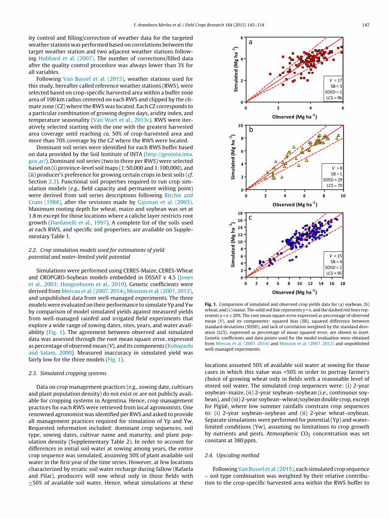

Crops Research 184 (2015) 145–154 147

iwtiaa

tsamataam

ogb(SuwCM1gam

2p

aedambfeadaaf

2

aapraRtudcwca≥

0 2 4 60

2

4

6

V = 17SB = 3

SDSD = 1LCS = 96

a

Observed (Mg ha-1)

Sim

ulat

ed (M

g ha

-1)

0 2 4 6 8 100

2

4

6

8

10

V = 8SB = 1

SDSD = 29LCS = 70

b

Observed (Mg ha-1)

Sim

ulat

ed (M

g ha

- 1)

0 2 4 6 8 10 12 14 16 1802468

1012141618

V = 15SB = 4

SDSD = 1LCS = 95

c

Observed (Mg ha-1)

Sim

ulat

ed (M

g ha

-1)

Fig. 1. Comparison of simulated and observed crop yields data for (a) soybean, (b)wheat, and (c) maize. The solid red line represents y = x, and the dashed red lines rep-resents y = x ± 20%. The root mean square error expressed as percentage of observedmean (V), and its components: squared bias (SB), squared difference betweenstandard deviations (SDSD), and lack of correlation weighted by the standard devi-ation (LCS), expressed as percentage of mean squared error, are shown in inset.

F. Aramburu Merlos et al. / Field

ty control and filling/correction of weather data for the targetedeather stations was performed based on correlations between the

arget weather station and two adjacent weather stations follow-ng Hubbard et al. (2007). The number of corrections/filled datafter the quality control procedure was always lower than 3% forll variables.

Following Van Bussel et al. (2015), weather stations used forhis study, hereafter called reference weather stations (RWS), wereelected based on crop-specific harvested area within a buffer zonerea of 100 km radius centered on each RWS and clipped by the cli-ate zone (CZ) where the RWS was located. Each CZ corresponds to

particular combination of growing degree days, aridity index, andemperature seasonality (Van Wart et al., 2013c). RWS were iter-tively selected starting with the one with the greatest harvestedrea coverage until reaching ca. 50% of crop-harvested area andore than 70% coverage by the CZ where the RWS were located.Dominant soil series were identified for each RWS buffer based

n data provided by the Soil Institute of INTA (http://geointa.inta.ov.ar/). Dominant soil series (two to three per RWS) were selectedased on (i) province-level soil maps (1:50,000 and 1:100,000), andii) producer’s preference for growing certain crops in best soils (cf.ection 2.3). Functional soil properties required to run crop sim-lation models (e.g., field capacity and permanent wilting point)ere derived from soil series descriptions following Ritchie andrum (1988), after the revisions made by Gijsman et al. (2003).aximum rooting depth for wheat, maize and soybean was set at

.8 m except for those locations where a caliche layer restricts rootrowth (Dardanelli et al., 1997). A complete list of the soils usedt each RWS, and specific soil properties, are available on Supple-entary Table 1.

.2. Crop simulation models used for estimations of yieldotential and water-limited yield potential

Simulations were performed using CERES-Maize, CERES-Wheatnd CROPGRO-Soybean models embedded in DSSAT v 4.5 (Jonest al., 2003; Hoogenboom et al., 2010). Genetic coefficients wereerived from Mercau et al. (2007, 2014), Monzon et al. (2007, 2012),nd unpublished data from well-managed experiments. The threeodels were evaluated on their performance to simulate Yp and Yw

y comparison of model simulated yields against measured yieldsrom well-managed rainfed and irrigated field experiments thatxplore a wide range of sowing dates, sites, years, and water avail-bility (Fig. 1). The agreement between observed and simulatedata was assessed through the root mean square error, expresseds percentage of observed mean (V), and its components (Kobayashind Salam, 2000). Measured inaccuracy in simulated yield wasairly low for the three models (Fig. 1).

.3. Simulated cropping systems

Data on crop management practices (e.g., sowing date, cultivarsnd plant population density) do not exist or are not publicly avail-ble for cropping systems in Argentina. Hence, crop managementractices for each RWS were retrieved from local agronomists. Oneenowned agronomist was identified per RWS and asked to providell management practices required for simulation of Yp and Yw.equested information included: dominant crop sequences, soilype, sowing dates, cultivar name and maturity, and plant pop-lation density (Supplementary Table 2). In order to account forifferences in initial soil water at sowing among years, the entirerop sequence was simulated, assuming 50% of plant available soil

ater in the first year of the time series. However, at few locations

haracterized by erratic soil water recharge during fallow (Rafaeland Pilar), producers will sow wheat only in those fields with50% of available soil water. Hence, wheat simulations at these

Genetic coefficients and data points used for the model evaluation were obtainedfrom Mercau et al. (2007, 2014) and Monzon et al. (2007, 2012) and unpublishedwell-managed experiments.

locations assumed 50% of available soil water at sowing for thosecases in which this value was <50% in order to portray farmer’schoice of growing wheat only in fields with a reasonable level ofstored soil water. The simulated crop sequences were: (i) 2-yearsoybean–maize, (ii) 2-year soybean–soybean (i.e., continuous soy-bean), and (iii) 2-year soybean–wheat/soybean double crop, exceptfor Pigüé, where low summer rainfalls constrain crop sequencesto: (i) 2-year soybean–soybean and (ii) 2-year wheat–soybean.Separate simulations were performed for potential (Yp) and water-limited conditions (Yw), assuming no limitations to crop growthby nutrients and pests. Atmospheric CO2 concentration was setconstant at 380 ppm.

2.4. Upscaling method

Following Van Bussel et al. (2015), each simulated crop sequence– soil type combination was weighted by their relative contribu-tion to the crop-specific harvested area within the RWS buffer to

148 F. Aramburu Merlos et al. / Field Crops Research 184 (2015) 145–154

F numerals within delineated climate zones), reference weather stations (closed triangles),a harvest area density per department (HAD, % of total department area) for the 2006–2012t

rcssAttwCRRYwtY

2p

bYec

A

wc

0 2 4 6 8 100

2

4

6

8

10

Maize

SoybeanWheat

Ya GYGA (Mg ha-1)

YaM

A(M

gha

- 1)

Fig. 3. National average actual yields (Ya) reported by the Argentine AgriculturalMinistry (MA, Mg ha−1) as a function of national Ya estimated through the upscaling

ig. 2. Maps of Argentina showing (a) selected climate zones (designated by Romannd buffer zones (hatched areas); and (b) soybean, (c) wheat, and (d) maize average

ime period.

etrieve averages Yw and Yp. For soybean, separate averages werealculated for single soybean (i.e., a full-season soybean crop) andoybean as the second crop of a double cropping sequence (i.e.,oybean sown immediately after harvest of a winter cereal crop).nnual Ya was calculated for each RWS based on the Ya reported for

he departments located within the RWS buffer and relative con-ribution of each department to total crop-specific harvested areaithin the RWS buffer. Finally, Yp, Yw, and Ya were upscaled toZ and country levels, based on the relative contribution of eachWS to total crop-specific harvested area. For all spatial scales (i.e.,WS, CZ, and country), Yg was calculated as the difference betweenw and Ya, and also expressed as percentage of Yw. The degree tohich crops are limited by water, i.e., the WLI, was calculated as

he difference between Yp and Yw and expressed as percentage ofp.

.5. National estimation of attainable crop production and ENSOhenomenon

Attainable yield was estimated to be 80% of water-limited yieldecause farmers’ yields tend to plateau when they reach 75–85% ofp or Yw (Cassman et al., 2010; Van Ittersum et al., 2013; Sadrast al., 2015). Attainable crop production (ACP) of Argentina wasalculated as follows:

CP = (Yw × 0.8) × Area

here area is the crop-specific harvested area of the last (2011/12)ropping season analyzed.

method of the Global Yield Gap Atlas Protocol followed in the present study (GYGA,Mg ha−1) for each of the 2005/06 to 2011/12 crop seasons. The solid line representsy = x.

In order to assess influence of the ENSO phenomenon onArgentine Ya, Yw and ACP, cropping seasons were categorized inENSO phases: Neutral, El Nino (typically wet years), and La Nina(typically dry years), based on the Oceanic Nino Index (ONI) ofthe Climate Prediction Center of NOAA’s National Weather Service

(2015). Yw and ACP differences between ENSO phases were eval-uated using non-parametric tests (Kruskal–Wallis and Levene’stests), while the effects on Ya were assessed by analyzing the resid-uals obtained from the regression analysis between Ya and year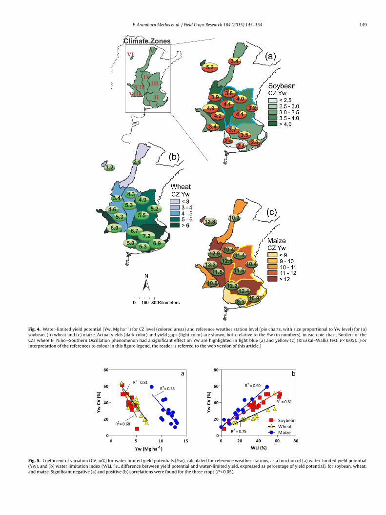

F. Aramburu Merlos et al. / Field Crops Research 184 (2015) 145–154 149

Fig. 4. Water-limited yield potential (Yw, Mg ha−1) for CZ level (colored areas) and reference weather station level (pie charts, with size proportional to Yw level) for (a)soybean, (b) wheat and (c) maize. Actual yields (dark color) and yield gaps (light color) are shown, both relative to the Yw (in numbers), in each pie chart. Borders of theCZs where El Nino—Southern Oscillation phenomenon had a significant effect on Yw are highlighted in light blue (a) and yellow (c) (Kruskal–Wallis test, P < 0.05). (Forinterpretation of the references to colour in this figure legend, the reader is referred to the web version of this article.)

0 5 10 150

20

40

60

80

R2= 0.55R2= 0.81

R2= 0.68

Yw (Mg ha-1)

YwCV

(%)

0 20 40 60 800

20

40

60

80

MaizeWheatSoybean

R2 = 0.90

R2 = 0.81

R2 = 0.75

WLI (%)

YwCV

(%)

a b

Fig. 5. Coefficient of variation (CV, in%) for water limited yield potentials (Yw), calculated for reference weather stations, as a function of (a) water-limited yield potential(Yw), and (b) water limitation index (WLI, i.e., difference between yield potential and water-limited yield, expressed as percentage of yield potential), for soybean, wheat,and maize. Significant negative (a) and positive (b) correlations were found for the three crops (P < 0.05).

1 Crops Research 184 (2015) 145–154

(y

3

3

dsadrasmfmiV2

3

3(r(uTasfhw

3p

asise8(HRcaewbhcbs

v(Riad

-50 0 50 10 0 15 0 20 0 25 00

20

40

60

80

SoybeanWheatMaize

R2= 0.55R2= 0.57

R2= 0.33

Yield gain rate (kg ha-1 y-1)

Yg(%

)

Fig. 6. Yield gaps (Yg, 2006–2012 average) at each reference weather station as afunction of yield gain rate (kg ha−1 y−1) from 1992 to 2012 for soybean, wheat andmaize. Significant negative correlations were found for the three crops (P < 0.05).Soybean values for CZ I showed a different pattern of Yg because of a severe water

50 F. Aramburu Merlos et al. / Field

both absolute residuals and relative to the Ya estimated for eachear).

. Results

.1. Selected weather stations and crop area coverage

Harvested soybean and maize area averaged 17.2 and 3 Mhauring the 2006–2012 period, respectively. Spatial distribution ofoybean and maize area was remarkably similar, with highest croprea density in the central Pampas (Fig. 2). In contrast, wheat pro-uction area (4.5 Mha) was concentrated in the southern Pampas. Aelatively small number of RWS buffers (16 for soybean and wheat,nd 15 for maize) was sufficient to cover 53, 50 and 48% of nationaloybean, wheat and maize harvested area, respectively. Further-ore, the eight CZ where the selected RWS were located accounted

or 81, 70 and 78% of total national crop area for soybean, wheat, andaize, respectively (Fig. 2). Five of these climate zones are located

n the Pampas (CZ I– IV and VII), two in the Chaco region (CZ VI andII), and one in the Espinal (CZ VIII) (Hall et al., 1992; Viglizzo et al.,011b).

.2. Variation in actual yields across Argentina

National average Ya calculated by the upscaling method was 2.7,.0, and 6.8 Mg ha−1 for soybean, wheat and maize, respectivelyTable 1). These values were in agreement with the national Yaeported by the Argentine Agricultural Ministry for the three cropst-test, P > 0.45), indicating the robustness of the method used topscale results from RWS buffers to larger geographic areas (Fig. 3).here was a large variation in Ya across RWS buffers in Argentina as

result of the large spatial variation in climate, soils and croppingystems (Supplementary Table 3–5). For instance, maize Ya rangedrom 3.2 to 8.9 Mg ha−1 across RWS (Supplementary Table 5). Theighest maize and soybean Ya were observed in the central Pampas,hile the highest wheat Ya was observed in the southeast Pampas.

.3. Spatial and temporal variation in water-limited yieldotential

National Yw was 3.9, 5.2, and 11.6 Mg ha−1 for soybean, wheatnd maize, respectively (Table 1). Wheat Yw was highest in theoutheast and decreased towards the northwest from 6.9 Mg ha−1

n CZ II to 2.1 Mg ha−1 in CZ V (Fig. 4b). Maize Yw was moretable across regions, ranging between 10.0 and 13.2 Mg ha−1,xcept in CZ I (i.e., southwest Pampas) where it barely exceeded.1 Mg ha−1 (Fig. 4c). The highest soybean Yw was found in the CZ VI5.2 Mg ha−1), which corresponds to the sub-humid Chaco region.owever, Yw in CZ VI might have been overestimated since theWS was located in the western edge of its crop area, where pre-ipitation is higher. CZ VII, IV and III, in central and west Pampas,lso presented high soybean Yw, of ca. 4.0 Mg ha−1 (Fig. 4a). Low-st soybean Yw was found in the southwest Pampas (2.2 Mg ha−1),hich is consistent with the results for maize. Second crop soy-

ean Yw was consistently lower than single soybean crop Yw, withigher differences in the south (up to 30%) than in the northernlimate zones (Supplementary Table 3). Likewise, soybean dou-le crop showed higher year-to-year variation in Yw than singleoybean crop (Supplementary Table 3).

For most RWS, low Yw was associated with high inter-annualariability in Yw and vice versa (Fig. 5a). Variation in water supplysoil water content at sowing plus in-season precipitation) across

WS explained the previous relationship, as indicated by the pos-

tive correlation between the coefficient of variation (CV) for Ywnd the WLI (Fig. 5b). The WLI may also reflects differences in pro-ucer’s preference to grow certain crops in best soils. For example,

limitation, and are indicated as *.

the WLI of soybean and maize in CZ I were different (61 versus 49%,respectively), which may be related to producer’s choice to growmaize in the best soils (Supplementary Table 1).

3.4. Spatial and temporal variation in yield gaps for soybean,wheat and maize in Argentina

Average Yg in Argentina was 1.3, 2.1, and 4.8 Mg ha−1 for soy-bean, wheat and maize, respectively (Table 1). Yg, expressed aspercentage of Yw, was remarkably smaller for soybean (32%) thanfor wheat and maize (41%), and this difference was consistentacross RWS (Fig. 4). Yg of the three crops varied widely within thecountry, ranging from 22 to 69% of the Yw across CZ. Despite suchvariability, there was no consistent correlation between Yg and Yw,Ya or yield CVs (P > 0.45). In general, largest gaps were found in areasthat had been recently converted into annual crop production whilesmallest gaps were found in those areas with long agricultural his-tory. The highest Yg (45 to 69% of Yw) were found in climate zonesV and VI, which are located in the Chaco region (Fig. 4). Western cli-mate zones (i.e., VII and VIII) also exhibited large gaps, ranging from40 to 60% of the Yw. Small Yg were found in central Pampas (i.e., cli-mate zones III and IV), reaching ca. 25% (for soybean) and between30 and 40% (for maize and wheat) of the Yw. The southern CZ (i.e., Iand II) had intermediate Yg for maize and wheat (ca. 40% of Yw), butwith a sharp longitudinal gradient, with decreasing Yw and increas-ing variability from east to west, due to a parallel decrease in rainfalltogether with an increasing frequency of soils where a caliche layerlimits the rooting depth (Monzon et al., 2012). Interestingly, soy-bean crops in CZ I had the lowest Yw, with the highest inter-annualvariability, but the lowest yield gap (Supplementary Table 3). Therewas a significant negative relationship (P < 0.05) between the sizeof the Yg and yield gain rates observed during the last 20 years ana-lyzed (1992–2012), suggesting that technological improvement incrop practices have not homogenously reached and/or impactedthe entire Argentine grain production area(Fig. 6).

Interestingly, magnitude of Yg at RWS, CZ, and national scalesdepended upon year (Fig. 7a). For the three crops, Ya approachedYw in dry years (i.e., in years with a high WLI), while Yg was signif-icantly higher in wet years (Fig. 7b). The contrasting pattern in wetversus dry years, which was consistent at all spatial levels, was in

agreement with the finding that the lowest soybean Yg occurred inthe most water-limited region (i.e., CZ I, Fig. 4).

F. Aramburu Merlos et al. / Field Crops Research 184 (2015) 145–154 151

Table 1Actual yields (Ya), water-limited yield potentials (Yw), yield gaps (Yg), and attainable crop production (ACP) for soybean, wheat and maize in Argentina based on 2011/12crop area. Actual yields are 7-y (2005/06–2011/12) averages. See Section 2.4 for details on calculation of ACP.

Ya (Mg ha−1)a Yw (Mg ha−1)a Yg (Mg ha−1)b Crop area (Mha) ACP (Mt)a

Soybean 2.65 (14%) 3.91 (18%) 1.26 (32%) 17.6 55 (18%)Wheat 3.02 (23%) 5.16 (21%) 2.14 (41%) 4.5 19 (21%)Maize 6.79 (18%) 11.60 (14%) 4.81 (41%) 3.7 34 (14%)

a Number between brackets shows the coefficient of variation (in%).b Number between brackets shows Yg as a percentage of Yw.

2006 200 8 2010 20 120

10

20

30

40

50

60a

Year

Yg(%

)

0 20 40 60 800

10

20

30

40

50

60

MaizeWheatSoybeanb

WLI (%)

Yg(%

)

Fig. 7. Argentine yield gaps (Yg) for each cropping season (2006–2012), expressed as percentage of water-limited yields, for soybean, wheat and maize, as a function of: (a)harvest year and (b) water limitation index (WLI, i.e., difference between yield potential apotential). A significant negative correlation was found between Yg and WLI for the threeamong crops (P > 0.46).

1985 1990 19 95 200 0 2005 201 0 20151

2

3

4

Year

Ya

(Mg

ha-1

)

-30

-20

-10

0

10

20

30

1985 1990 1995 200 0 200 5 2010 201 52

4

6

8

10

El NiñoNeutralLa Niña

Yea r

Ya

(Mg

ha-1

)

-30

-20

-10

0

10

20

30

a

b

Fig. 8. Trends in actual yield (Ya) from 1985 to 2015 in Argentina as related toETbs

3c

b

average Yg calculated for the 2006–2012 period (32 to 41% of Yw

l Nino—Southern Oscillation phenomenon (ENSO) for soybean (a) and maize (b).he insets show the relative Ya residuals (%) obtained from the regression analysisetween Ya and year. For maize, there was a significant difference between thelopes of the relative residuals of El Nino and La Nina phases over time (P < 0.05).

.5. ENSO phenomenon effect on Argentine actual and attainable

rop production

In relative terms, the effects of the ENSO phenomenon on soy-ean Ya was constant over time (Fig. 8a), while there was an

nd water-limited yield for each cropping season, expressed as percentage of yield crops (P < 0.05), with no significant differences in the linear regression parameters

increasingly higher difference in maize Ya between ENSO phasesover time, both in absolute and relative terms (Fig. 8b). Wheat Yawas not affected by the ENSO phenomenon.

Yield gap closure to a level of 20% of Yw would lead Argentinato a production of 55, 19, and 34 Mt of soybean, wheat, andmaize, respectively, without expansion in cropland area (Table 1).However, national Yw, and hence ACP varied significantly amongyears because of climate variability, with CV ranging from 14 to21%. Inter-annual variation in summer crops ACP were partiallyexplained by the influence of the ENSO phenomenon. During “LaNina” years, Argentine maize ACP was significantly lower andmore variable than during “El Nino” and Neutral years (P < 0.05,Fig. 9). Likewise, soybean ACP was higher in “El Nino” years andlower in “La Nina” years (P < 0.05), with no significant variation inthe inter-annual variability within each phase (Fig. 9). The ENSOphenomenon had a strong effect on summer crops Yw and cropproduction in a limited but highly productive region of Argentina(i.e., CZ III and IV for soybean, and II and III for maize, Fig. 4). On theother hand, the ENSO phenomenon did not have a clear influencein wheat ACP (P = 0.72).

4. Discussion

Argentina is one of the major grain exporter countries sinceearly 20th century. Assuming a standard nutritional unit of 500 kggrain equivalent per capita per year (Connor et al., 2011), Argentinaproduces enough grain to feed ca. 200 million people, that is, fivetimes its current population. In addition, Argentina could havepotentially produced an extra 7.4 Mt of soybean, 5.2 Mt of wheatand 9.2 Mt of maize on existing cropland area, by closing national

depending upon crop) to an attainable level of 20% of Yw. If theextra crop production amount achieved through yield gap closurehad been exported, which was very likely given the low internaldemand, it would have represented an increase in soybean, wheat

152 F. Aramburu Merlos et al. / Field Crops

El Niñ o Neutral La Niña20

25

30

35

40

45Maize

a a

b*

ENSO phase

20

30

40

50

60

70

80Soybeana

ab b

5

10

15

20

25

30Whe at

A�ai

nabl

e Cr

op P

rodu

c�on

(Mt)

Fig. 9. Attainable soybean, wheat and maize production of Argentina as affected by“El Nino”—Southern Oscillation phenomenon (ENSO) based on 2011/12 crop area.Different letters, within the same panel, indicate significant differences among ENSOphases at P < 0.05 (Kruskal–Wallis test). Distance between horizontal dashed linesrepresents 10% of global exports for each crop (2006–2011 average, FAOSTAT 2015).Attainable maize production in La Nina years presented a significant higher variance(p

aifddeogoweeaatApa

Levene’s test, P < 0.05). See Section 2.4 for details on calculation of attainable croproduction.

nd maize global exports of a respective 9%, 4% and 9%.2 In turn, thisncrease in global exports would have been sufficient to cover theood requirements of 44 million people. However, Argentine pro-uction and its contribution to global grain markets greatly variesue to climate variation as related to ENSO phenomenon (Podestát al., 1999; Iizumi et al., 2014). Furthermore, the reported effectsf the ENSO phases on Argentine maize production tended to bereater during the last cropping seasons (Fig. 8), despite incrementsf late-sown maize, which has lower Yp than early sowings, butith significant reductions in Yw CV (Maddonni, 2012; Mercau

t al., 2014). This pattern might reflect that attainable yields areven more sensible to the ENSO phenomenon than Ya, and, as Yapproaches Yw, the former will become more variable, if crop man-gement practices do not change. For example, in “La Nina” yearshere is a high probability of widespread droughts that may reducergentine maize production capacity by more than 30%, with a

arallel 10% impact on global maize exports. Likewise, averagettainable soybean production in “La Nina” years is 12 Mt lower

2 Global exports were estimated from 2006 to 2011 averages (FAO, 2015).

Research 184 (2015) 145–154

than in “El Nino” years, which represents a reduction of globalexports of soybean by 15% (Fig. 9).

In a global context, size of Yg of major Argentine cerealcrops is moderate. Wheat and maize Yg in Argentina represented41% of their respective Yw, which were similar to those esti-mated for sunflower by Hall et al. (2013), but considerably higherthan the gaps reported for some major high-technology cereal-producing regions, e.g.,wheat in Germany and maize in Nebraska,USA, which had gaps of ∼20% (Grassini et al., 2011; Van Wartet al., 2013b). At the other extreme, Yg in Argentina were muchsmaller than those reported for smallholder production systemsin Sub-Saharan Africa (Tittonell and Giller, 2013; Kassie et al.,2014). Considering an ‘S-shaped curve’ production function inresponse to inputs (De Wit, 1992), African smallholder agricultureare located at the low-input/low-response zone, and the high tech-nology cereal-producing regions are at the high-input/plateau zone(Tittonell, 2013). Argentine cropping systems are between thesetwo extremes, within the ‘high-response zone’, but with high vari-ability among regions and farmers. This could partially explain thehigh rate of crop yield increase that Argentina had during the lasttwenty years. In fact, Argentina is one of the few countries exhibit-ing rates of yield increase that are sufficient to double current cropproduction by 2050, though this will only be achieved if currentrates of yield gain are sustained over the next 35 years (Ray et al.,2013). Even with no changes in current Yw, if Argentina is ableto sustain its current yield gain rates, the average national Ya willreach 80% of Yw by 2025, 2026 and 2038 for soybean, maize andwheat, respectively. Moreover, there is evidence that Yw and landproductivity can be further increased in Argentina. For example,farmers are adopting concepts on zone management, climate fore-casts (as related to ENSO), and in-season measurement (like soilwater at sowing) to fine tune crop management (Bert et al., 2006;Monzon et al., 2007; Peralta et al., 2013), while land productiv-ity can be increased by intensifying crop sequences in the Pampas(Monzon et al., 2014; J.F. Andrade et al., 2015).

Soybean Yg is considerably lower than Yg of maize and wheat inArgentina (32% versus 41% of Yw). This difference can be explainedby: (i) higher vegetative and reproductive plasticity of soybeanrelative to maize (Andrade, 1995); (ii) Argentine soybean cropsobtained ca. 60% of their N from biological N fixation (Collino et al.,2015), (iii) the requirement of P to reach 90% of the maximumyield for soybean is considerably lower than for wheat and maize(Hanway and Olson, 1980). Crops are typically nutrient-limitedin Argentina, as the rates of fertilizers applied have increasedbut are still low relative to crop nutrient requirements (Calvinoand Monzon, 2009; Lavado and Taboada, 2009), resulting in neg-ative nutrient balances (Liu et al., 2010; MacDonald et al., 2011;Lassaletta et al., 2014). Considering that wheat, maize and sun-flower Yg were remarkably similar, and 10% higher than soybeanYg, it is likely that these differences can be partly related to nitrogendeficiencies.

Argentina is not only an interesting case of study for its greatpotential for crop production and grain exports, but also for itsgreat cropping system variability among regions which resultedin a wide range of Yw, Yg (Fig. 4) and year-to-year variation (Fig. 7).This variability had not been properly quantified in previous Ygassessments, mainly because these were global studies that didnot account for spatial variation on soil and crop managementwithin the country, or made no attempt to use yearly weatherdata, or were based on coarse weather, soil, and management data(Neumann et al., 2010; Licker et al., 2010; Foley et al., 2011; Muelleret al., 2012). For example, Neumann et al. (2010) roughly agreed

with our national estimates of wheat and maize Yg, but such workwas not sensitive enough to detect regional variations, whereasLicker et al. (2010) and Foley et al. (2011) grossly underestimatedArgentine maize and soybean Yw. It has been suggested that Yg are

Crops

hheiasoccolyFecitati

fayLBYhosltssbtfralmhYsrie

5

Ad9psmyygtgy

F. Aramburu Merlos et al. / Field

igher when the risk associated to crop production is greater, i.e.,igh coefficient of variation for yield (Fischer et al., 2009). Inter-stingly, despite the high variation in Yw, Ya and yield CVs foundn Argentina, there was no correlation between any of these vari-bles and the Yg. Other variables are likely to explain better thepatial variation on Yg, for example, crop history (i.e., the numberf years that a given region has been under commercial-scale agri-ulture) and technology level applied by farmers (Fig. 6). Indeed, wean distinguish contrasting scenarios for major agricultural regionsf Argentina. In the Chaco region (i.e., CZ V and VI), the Yg wasargest probably because of the recent agriculture history and smallield gain rates observed during the last twenty years (1992–2012).uture efforts on research should be made to understand the socio-conomic factors that explain low yield gains in this region. At theentral Pampas (i.e., CZ III and IV), farmer’s yields have significantlyncreased during the last 20 years and Yg tends to be lower than inhe rest of the country. Since farmer’s yield will reach the attain-ble yield in the medium-term, future on-farm yield increase inhis region might rely on increases in Yw of individual crops orncreasing crop intensity, or both.

The present study clearly shows that Yg varied significantlyrom year to year (Fig. 7). The temporal variation in Yg, which isn aspect that has not been analyzed in previous yield gap anal-ses, can bring some light on yield gap causes (Hall et al., 2013;aborte et al., 2012; Van Rees et al., 2014; Van Wart et al., 2013b).oth Yw and Ya followed the same trend across years; however,w was more sensitive to wet years, relative to Ya, resulting inigher Yg in the more favorable wet years (Fig. 7b). In wet years,ther non-water related factors became limiting, such as nutrientupply or incidence of insect, pests and pathogens, resulting in aarge gap between Yw and Ya. In contrast, in dry years, water washe most limiting factor for crop production, and Yg was relativelymaller. Likewise, a combination of low summer rainfall and lowoil water holding capacity were the major limiting factors for soy-ean yields in CZ I, hence, it was not surprising that soybean Yg washe lowest in this region (Fig. 4). The contrasting behavior of Yg inavorable versus non-favorable years might be related to farmer’sisk aversion behavior and its impact on the level of applied inputsnd technology. Specifically, since the level of applied inputs isikely to be determined based on the yield reached with normal or

oderately adverse weather conditions, current management mayave an unintended opportunity cost in favorable years with highw. Availability of ENSO-related climate forecasts and other early-eason indicators (such as soil water content at sowing) can help toeduce the uncertainties associated with crop production, allow-ng farmers to take advantage of the favorable years and reduce theconomic loses in adverse years (Bert et al., 2006).

. Conclusions

Yield gap assessment performed in this study indicates thatrgentina had the potential to substantially increase grain pro-uction of soybean, wheat and maize, by a respective 7.4, 5.2 and.2 Mt, without expanding cropland area. This potential grain sur-lus would have a great impact on grain global exports, but withignificant variations across years because of the inter-annual cli-ate variability related to the ENSO phenomenon. Magnitude of

ield gap in Argentina depended upon year, with largest Yg in wetears and smallest Yg in dry years. Substantial variation in yield

aps was found across crop producing regions, which highlightshe usefulness of the spatial framework applied in this study to tar-et research and, ultimately, reduce gaps in areas where currentield is well below its potential.

Research 184 (2015) 145–154 153

Acknowledgments

We are grateful to local agronomists in Argentina who pro-vided data on management practices: Agustín Giorno (AsociaciónArgentina de Consorcios Regionales de Experimentación Agrí-cola, AACREA), Alberto Quiroga (INTA), Eduardo Martínez Quiroga(AACREA), Fernando Ross (INTA), Juan Martín Capelle (AACREA), LíaOlmedo Pico (INTA), Martín Sanchez (AACREA), Octavio Caviglia(INTA), and Pablo Calvino (AACREA). We also thank Hugo GrossiGallegos (University of Lujan) for providing measured solar radia-tion data. This work is part of a thesis by Fernando Aramburu Merlosin partial fulfillment for the M. Sc. degree (Universidad Nacional deMar del Plata). This project was supported by the Daugherty Waterfor Food Institute at University of Nebraska-Lincoln.

Appendix A. Supplementary data

Supplementary data associated with this article can be found, inthe online version, at http://dx.doi.org/10.1016/j.fcr.2015.10.001.

References

Alexandratos, N., Bruinsma, J., 2012. World Agriculture Towards 2030/2050: The2012 Revision. ESA Working Paper Rome, FAO.

Andrade, F.H., 1995. Analysis of growth and yield of maizesunflower and soybeangrown at Balcarce. Argent. Field Crops Res. 41, 1–12.

Andrade, F.H., Sala, R., Pontaroli, A., León, A., Castro, S., 2015. Integration ofbiotechnology, plant breeding and crop physiology. Dealing with complexinteractions from a physiological perspective. In: Sadras, V., Calderini, D. (Eds.),Crop Physiology: Applications for Genetic Improvement and Agronomy.Elsevier Science, New York, pp. 487–503.

Andrade, J.F., Poggio, S.L., Ermácora, M., Satorre, E.H., 2015. Productivity andresource use in intensified cropping systems in the Rolling Pampa. Argent. Eur.J. 67, 37–51, http://dx.doi.org/10.1016/j.eja.2015.03.001.

Bert, F.E., Satorre, E.H., Toranzo, F.R., Podestá, G.P., 2006. Climatic information anddecision-making in maize crop production systems of the ArgentineanPampas. Agric. Syst. 88, 180–204.

Bruinsma, J., 2009. The resource outlook to in Expert Meeting on How to Feed theWorld in 2050.

Calvino, P., Monzon, J.P., 2009. Farming systems of Argentina: yield constraints andrisk management. In: Sadras, V.O., Calderini, D. (Eds.), Crop Physiology:Applications for Genetic Improvement and Agronomy. Academic Press,Elsevier, pp. 55–67.

Cassman, K.G., Dobermann, A., Walters, D.T., Yang, H., 2003. Meeting cerealdemand while protecting natural resources and improving environmentalquality. Annu. Rev. Environ. Resour. 28, 315–358.

Cassman, K.G., Grassini, P., van Wart, J., 2010. Crop yield potential, yield trends,and global food security in a changing climate. In: Rosenzweig, C., Hillel, D.(Eds.), Handbook of Climate Change and Agroecosystems. Imperial CollegePress, London, pp. 37–51.

Collino, D.J., Salvagiotti, F., Perticari, A., Piccinetti, C., Ovando, G., Urquiaga, S.,Racca, R.W., 2015. Biological nitrogen fixation in soybean in Argentina:relationships with crop, soil, and meteorological factors. Plant Soil, 1–14.

Connor, D.J., Loomis, R.S., Cassman, K.G., 2011. Crop Ecology. Production andManagement in Agricultural Systems. CUP, Cambridge, UK.

Dardanelli, J.L., Bachmeier, O.A., Sereno, R., Gil, R., 1997. Rooting depth and soilwater extraction patterns of different crops in a silty loam haplustoll. FieldCrops Res. 54, 29–38.

De Wit, C.T., 1992. Resource use efficiency in agriculture. Systems approaches foragricultural. Agric. Syst. 40, 125–151.

Evans, L.T., 1993. Crop Evolution, Adaptation and Yield. Cambridge UniversityPress, Cambridge, UK.

Evans, L.T., Fischer, R.A., 1999. Yield potential: its definition, measurement, andsignificance. Crop Sci. 39, 1544–1551.

FAOSTAT, FAO, 2015. Retrieved April.Fermont, A., van Van Asten, P.J.A., Tittonell, P., Van Wijk, M.T., Giller, K.E., 2009.

Closing the cassava yield gap: an analysis from smallholder farms in EastAfrica. Field Crops Res 112, 24–36.

Fernández-Long, M.E., Müller, G.V., Beltrán-Przekurat, A., Scarpati, O.E., 2013.Long-term and recent changes in temperature-based agroclimatic indices inArgentina. Int. J. Climatol 33, 1673–1686.

Fischer, R.A., Byerlee, D., Edmeades, G.O., 2009. Can Technology Deliver on theYield Challenge to 2050. In: Expert Meeting on How to Feed the World in 2050.FAO, Rome, pp. 389–462.

Fischer, T., Byerlee, D., Edmeades, G.O., 2014. Crop Yields and Global Food Security:

Will Yield Increase Continue to Feed the World? ACIAR Monograph. Australiancentre for international agricultural research, Cranberra.

Foley, J.A., Ramankutty, N., Brauman, K.A., Cassidy, E.S., Gerber, J.S., Johnston, M.,Mueller, N.D., O’Connell, C., Ray, D.K., West, P.C., Balzer, C., Bennett, E.M.,Carpenter, S.R., Hill, J., Monfreda, C., Polasky, S., Rockström, J., Sheehan, J.,

1 Crops

G

G

G

G

H

H

H

H

H

I

J

K

K

L

L

L

L

L

L

L

M

M

M

M

M

54 F. Aramburu Merlos et al. / Field

Siebert, S., Tilman, D., Zaks, D.P.M., 2011. Solutions for a cultivated planet.Nature 478, 337–342.

ijsman, A.J., Jagtap, S.S., Jones, J.W., 2003. Wading through a swamp of completeconfusion: how to choose a method for estimating soil water retentionparameters for crop models. Eur. J. Agron 18, 77–106.

rassini, P., Eskridge, K.M., Cassman, K.G., 2013. Distinguishing between yieldadvances and yield plateaus in historical crop production trends. Nat.Commun., 4.

rassini, P., Thorburn, J., Burr, C., Cassman, K.G., 2011. High-yield irrigated maize inthe Western US Corn Belt: I. On-farm yield, yield potential, and impact ofagronomic practices. Field Crops Res. 120, 142–150.

rassini, P., van Bussel, L.G., Van Wart, J., Wolf, J., Claessens, L., Yang, H., Boogaard,H., de Groot, H., van Ittersum, M.K., Cassman, K.G., 2015. How good is goodenough? Data requirements for reliable crop yield simulations and yield-gapanalysis. Field Crops Res. 177, 49–63, 10.1016/j.fcr.2015.03.004.

all, A.J., Feoli, C., Ingaramo, J., Balzarini, M., 2013. Gaps between farmer andattainable yields across rainfed sunflower growing regions of Argentina. FieldCrops Res. 143, 119–129, Crop Yield Gap Analysis—Rationale, Methods andApplications.

all, A.J., Rebella, C.M., Ghersa, C.M., Culot, J.P., 1992. Field-crop systems of thePampas. In: Field Crop Ecosystems of the World. Elsevier, Exeter, UK, pp.413–450.

anway, J.J., Olson, R.A., 1980. Phosphate nutrition of corn, sorghum, soybeans,and small grains. In: Khasawneh, F.E., Sample, E.C., Kamprath, E.J. (Eds.), TheRole of Phosphorus in Agriculture. ASA, Madison, WI, pp. 681–692.

oogenboom, G., Jones, J.W., Wilkens, P.W., Porter, C.H., Boote, K.J., Hunt, L.A.,et al., 2010. Decision Support System for Agrotechnology Transfer (DSSAT)Version 4.5.[CD-ROM]. Univ. of Hawaii, Honolulu.

ubbard, K.G., Guttman, N.B., You, J., Chen, Z., 2007. An improved QC process fortemperature in the daily cooperative weather observations. J. Atmos. OceanTechnol., 24.

izumi, T., Luo, J.-J., Challinor, A.J., Sakurai, G., Yokozawa, M., Sakuma, H., Brown,M.E., Yamagata, T., 2014. Impacts of El Nino Southern Oscillation on the globalyields of major crops. Nat. Commun., 5.

ones, J.W., Hoogenboom, G., Porter, C.H., Boote, K.J., Batchelor, W.D., Hunt, L.A.,Wilkens, P.W., Singh, U., Gijsman, A.J., Ritchie, J.T., 2003. The DSSAT croppingsystem model. Eur. J. Agron. 18, 235–265.

assie, B.T., Van Ittersum, M.K., Hengsdijk, H., Asseng, S., Wolf, J., Rötter, R.P., 2014.Climate-induced yield variability and yield gaps of maize (Zea mays L.) in theCentral Rift Valley of Ethiopia. Field Crops Res. 160, 41–53.

obayashi, K., Salam, M.U., 2000. Comparing simulated and measured values usingmean squared deviation and its components. Agron. J. 92, 345–352.

aborte, A.G., de Bie, K.C.A.J.M., Smaling, E.M.A., Moya, P.F., Boling, A.A., VanIttersum, M.K., 2012. Rice yields and yield gaps in Southeast Asia: past trendsand future outlook. Eur. J. Agron. 36, 9–20.

ambin, E.F., Gibbs, H.K., Ferreira, L., Grau, R., Mayaux, P., Meyfroidt, P., Morton,D.C., Rudel, T.K., Gasparri, I., Munger, J., 2013. Estimating the world’spotentially available cropland using a bottom-up approach. Glob. Environ.Change 23, 892–901.

assaletta, L., Billen, G., Grizzetti, B., Anglade, J., Garnier, J., 2014. 50 year trends innitrogen use efficiency of world cropping systems: the relationship betweenyield and nitrogen input to cropland. Environ. Res. Lett. 9, 105011, http://dx.doi.org/10.1088/1748-9326/9/10/105011.

avado, R.S., Taboada, M.A., 2009. The Argentinean Pampas: a key region with anegative nutrient balance and soil degradation needs better nutrientmanagement and conservation programs to sustain its future viability as aworld agroresource. J. Soil Water Conserv. 64, 150A–153A.

icker, R., Johnston, M., Foley, J.A., Barford, C., Kucharik, C.J., Monfreda, C.,Ramankutty, N., 2010. Mind the gap: how do climate and agriculturalmanagement explain the yield gap of croplands around the world? Glob. Ecol.Biogeogr. 19, 769–782.

iu, J., You, L., Amini, M., Obersteiner, M., Herrero, M., Zehnder, A.J.B., Yang, H.,2010. A high-resolution assessment on global nitrogen flows in cropland. Proc.Natl. Acad. Sci. U. S. A. 107, 8035–8040, http://dx.doi.org/10.1073/pnas.0913658107.

obell, D.B., Cassman, K.G., Field, C.B., 2009. Crop yield gaps: their importance,magnitudes, and causes. Annu. Rev. Environ. Resour. 34, 179–204.

acDonald, G.K., Bennett, E.M., Potter, P.A., Ramankutty, N., 2011. Agronomicphosphorus imbalances across the world’s croplands. Proc. Natl. Acad. Sci. 108,3086–3091.

addonni, G.A., 2012. Analysis of the climatic constraints to maize production inthe current agricultural region of Argentina—a probabilistic approach. Theor.Appl. Climatol. 107, 325–345, http://dx.doi.org/10.1007/s00704-011-0478-9.

ercau, J.L., Dardanelli, J.L., Collino, D.J., Andriani, J.M., Irigoyen, A., Satorre, E.H.,2007. Predicting on-farm soybean yields in the pampas usingCROPGRO-soybean. Field Crops Res. 100, 200–209.

ercau, J.L., Otegui, M.E., Ahuja, L.R., Ma, L., Lascano, R.J., 2014. A modelingapproach to explore water management strategies for late-sown maize anddouble-cropped wheat–maize in the rainfed Pampas region of Argentina. In:Ahuja, L.R., Ma, L., Lascano, R.J. (Eds.), Practical applications of agriculturalsystem models to optimize the use of limited water. Adv. Agric. Systems

Model. 5. ASA, SSSA, CSSA, Madison, WI, pp. 351–374.

onzon, J.P., Mercau, J.L., Andrade, J.F., Caviglia, O.P., Cerrudo, A.G., Cirilo, A.G.,Vega, C.R.C., Andrade, F.H., Calvino, P.A., 2014. Maize-soybean intensificationalternatives for the Pampas. Field Crops Res. 162, 48–59, http://dx.doi.org/10.1016/j.fcr.2014.03.012.

Research 184 (2015) 145–154

Monzon, J.P., Sadras, V.O., Abbate, P.A., Caviglia, O.P., 2007. Modelling managementstrategies for wheat–soybean double crops in the south-eastern Pampas. FieldCrops Res. 101, 44–52.

Monzon, J.P., Sadras, V.O., Andrade, F.H., 2012. Modelled yield and water useefficiency of maize in response to crop management and Southern OscillationIndex in a soil—climate transect in Argentina. Field Crops Res. 130, 8–18.

Mueller, N.D., Gerber, J.S., Johnston, M., Ray, D.K., Ramankutty, N., Foley, J.A., 2012.Closing yield gaps through nutrient and water management. Nature 490,254–257.

Neumann, K., Verburg, P.H., Stehfest, E., Müller, C., 2010. The yield gap of globalgrain production. Spat. Anal. Agric. Syst. 103, 316–326.

Peralta, N.R., Costa, J.L., Balzarini, M., Angelini, H., 2013. Delineation ofmanagement zones with measurements of soil apparent electricalconductivity in the southeastern pampas. Can. J. Soil Sci. 93, 205–218, http://dx.doi.org/10.4141/CJSS2012-022.

Piesse, J., Thirtle, C., 2009. Three bubbles and a panic: an explanatory review ofrecent food commodity price events. Food Policy 34, 119–129.

Podestá, G.P., Messina, C.D., Grondona, M.O., Magrin, G.O., 1999. Associationsbetween grain crop yields in central-eastern Argentina and El Nino-SouthernOscillation. J. Appl. Meteorol. 38, 1488–1498.

Ray, D.K., Mueller, N.D., West, P.C., Foley, J.A., 2013. Yield trends are insufficient todouble global crop production by 2050. PLoS One 8, e66428.

Ritchie, J.T., Crum, J., 1988. Converting soil survey characterization data intoIBSNAT crop model input. In: Bouma, J., Bregt, A.K. (Eds.), Land Qualities inSpace and Time. Proceedings of a Symposium Organized by the InternationalSociety of Soil Science (ISSS). Wageningen, the Netherlands, 22–26 August1988. Pudoc, Wageningen, pp. 155–167.

Sadras, V.O., Cassman, K.G., Grassini, P., Hall, A.J., Bastiaansen, W.G.M., Laborte,A.G., Milne, A.E., Sileshi, G., Steduto, P., 2015. Yield Gap Analysis of Rainfed andIrrigated Crops: Methods and Case Studies. (Water Reports No. 41). Food andAgriculture Organization of the United Nations (FAO), Rome.

Sadras, V.O., Grassini, P., Costa, R., Cohan, L., Hall, A.J., 2014. How reliable are cropproduction data? Case studies in USA and Argentina. Food 6, 447–459, http://dx.doi.org/10.1007/s12571-014-0361-5.

Satorre, E.H., 2011. Recent changes in pampean agriculture: possible new avenuesin coping with global change challenges. In: Slafer, Araus (Eds.), Crop StressManagement and Global Climate Change; CABI Series No. 2, pp. 47–57.

Siebert, S., Henrich, V., Frenken, K., Burke, J., 2013. Update of the Digital Global Mapof Irrigation Areas to Version 5. Bonn: Institute of Crop Science and ResourceConservation Rheinische Friedrich-Wilhelms-Universität Bonn.

Tittonell, P., 2013. Farming Systems Ecology: towards Ecological Intensification ofWorld Agriculture. Wageningen University, Wageningen, pp. 40 p.

Tittonell, P., Giller, K.E., 2013. When yield gaps are poverty traps: the paradigm ofecological intensification in African smallholder agriculture. Field Crops Res.143, 76–90.

Trostle, R., 2010. Global Agricultural Supply and Demand: Factors Contributing tothe Recent Increase in Food Commodity Prices (rev. Ed.). DIANE Publishing.

Van Bussel, L.G., Grassini, P., Van Wart, J., Wolf, J., Claessens, L., Yan, H., Boogaard,H., de Groot, H., Saito, K., Cassman, K.G., Van Ittersum, M.K., 2015. From field toatlas: upscaling of location-specific yield gap estimates. Field Crops Res. 177,98–108, http://dx.doi.org/10.1016/j.fcr.2015.03.005.

Van Ittersum, M.K., Cassman, K.G., Grassini, P., Wolf, J., Tittonell, P., Hochman, Z.,2013. Yield gap analysis with local to global relevance—a review. Field CropsRes. 143, 4–17, http://dx.doi.org/10.1016/j.fcr.2012.09.009.

Van Ittersum, M.K., Rabbinge, R., 1997. Concepts in production ecology for analysisand quantification of agricultural input-output combinations. Field Crops Res.52, 197–208.

Van Rees, H., McClelland, T., Hochman, Z., Carberry, P., Hunt, J., Huth, N.,Holzworth, D., 2014. Leading farmers in South East Australia have closed theexploitable wheat yield gap: prospects for further improvement. Field CropsRes. 164, 1–11.

Van Wart, J., Grassini, P., Cassman, K.G., 2013a. Impact of derived global weatherdata on simulated crop yields. Glob. Change Biol. 19, 3822–3834, http://dx.doi.org/10.1111/gcb.12302.

Van Wart, J., Kersebaum, K.C., Peng, S., Milner, M., Cassman, K.G., 2013b. Estimatingcrop yield potential at regional to national scales. Field Crops Res. 143,34–43.

Van Wart, J., van Bussel, L.G., Wolf, J., Licker, R., Grassini, P., Nelson, A., Boogaard,H., Gerber, J., Mueller, N.D., Claessens, L., 2013c. Use of agro-climatic zones toupscale simulated crop yield potential. Field Crops Res. 143, 44–55.

Viglizzo, E.F., Frank, F.C., Carreno, L.V., Jobbagy, E.G., Pereyra, H., Clatt, J., Pincen, D.,Ricard, M.F., 2011a. Ecological and environmental footprint of 50 years ofagricultural expansion in Argentina. Glob. Change Biol. 17,959–973.

Viglizzo, E.F., Ricard, M.F., Jobbágy, E.G., Frank, F.C., Carreno, L.V., 2011b. Assessingthe cross-scale impact of 50 years of agricultural transformation in Argentina.Field Crops Res. 124, 186–194.

Volante, J.N., Alcaraz-Segura, D., Mosciaro, M.J., Viglizzo, E.F., Paruelo, J.M., 2012.Ecosystem functional changes associated with land clearing in NW Argentina.Agric. Ecosyst. Environ. 154, 12–22.

Waddington, S.R., Li, X., Dixon, J., Hyman, G., De Vicente, M.C., 2010. Getting the

focus right: production constraints for six major food crops in Asian andAfrican farming systems. Food Secur. 2, 27–48.

White, J.W., Hoogenboom, G., Wilkens, P.W., Stackhouse, P.W., Hoel, J.M., 2011.Evaluation of satellite-based,: modeled-derived daily solar radiation data forthe continental United States. Agron. J. 103, 1242–1251.