potential information fields for mobile robot … · potential information elds for mobile robot...

Potential information fields for mobile robot exploration

Joan Vallve, Juan Andrade-Cetto

Institut de Robotica i Informatica Industrial, CSIC-UPCLlorens Artigas 4-6, 08028 Barcelona, Spain.

Abstract

We present a decision theoretic approach to mobile robot exploration. Themethod evaluates the reduction of joint path and map entropy and computesa potential information field in robot configuration space using these joint en-tropy reduction estimates. The exploration trajectory is computed descendingon the gradient of these field. The technique uses Pose SLAM as its estimationbackbone. Very efficient kernel convolution mechanisms are used to evaluateentropy reduction for each sensor ray, and for each possible robot orientation,taking frontiers and obstacles into account. In the end, the computation of thisfield on the entire configuration space is shown to be very efficient computa-tionally. The approach is tested in simulations in a pair of publicly availabledatasets comparing favorably both in quality of estimates and in execution timeagainst an RRT*-based search for the nearest frontier and also against a locallyoptimal exploration strategy.

Keywords: Mobile robotics, SLAM, Exploration

1. Introduction

We consider the problem of autonomous mobile robot exploration, and frameit as that of reducing both localization and map uncertainties. Explorationstrategies driven by uncertainty reduction date back to the seminal work ofWhaite [21] for the acquisition of 3-D models of objects from range data. Withinthe context of SLAM, it is the work of Feder et al. [4], who first proposed a metricto evaluate uncertainty reduction as the sum of the independent robot and land-mark entropies with an exploration horizon of one step to autonomously produceoccupancy maps. Bourgault et al. [1] alternatively proposed a utility functionfor exploration that trades off the potential reduction of vehicle localization un-certainty, measured as entropy over a feature-based map, and the information

Email addresses: [email protected] (Joan Vallve), [email protected] (JuanAndrade-Cetto)

1This work has been supported by the Spanish Ministry of Economy and Competitivenessunder Project DPI-2011-27510 and by the EU Project Cargo-ANTs FP7-605598.

2This paper is an extended and revised version of [18].

Preprint submitted to Elsevier November 24, 2014

gained over an occupancy grid. In contrast to these approaches, which con-sider independently the reduction of vehicle and map entropies, Vidal-Callejaet al., [20] tackled the issue of joint robot and map entropy reduction, takinginto account robot and map cross correlations for the Visual SLAM EKF case.

Action selection in SLAM can also be approached as an optimization problemusing receding horizon strategies [6, 11, 10]. Multi-step look ahead explorationin the context of SLAM makes sense only for situations in which the concate-nation of prior estimates without measurement evidence remain accurate forlarge motion sequences. For highly unstructured scenarios and poor odometrymodels, this is hardly the case. So, we stick with the one step look ahead case.

One technique that tackles the problem of exploration in SLAM as a one steplook ahead entropy minimization problem makes use of Rao-Blackwellized par-ticle filters [15]. The technique extends the classical frontier-based explorationmethod [22] to the full SLAM case. When using particle filters for exploration,only a very narrow action space can be evaluated due to the complexity in com-puting the expected information gain. The main bottleneck is the generation ofthe expected measurements that each action sequence would produce, which isgenerated by a ray-casting operation in the map of each particle. In contrast,measurement predictions in a Pose SLAM implementation, such as ours, can becomputed much faster, having only one map posterior per action to evaluate,instead of the many that a particle filter requires. Moreover, in [15], the costof choosing a given action is subtracted from the expected information gainwith a user selected weighting factor. In our approach, the cost of long actionsequences is taken into consideration during the selection of goal candidates,using the same information metrics that help us keep the robot localized duringpath execution.

In [17] our group proposed a solution to the exploration problem that max-imizes information gain in both the map and path estimates. The methodevaluates both exploratory and loop closure candidate trajectories, computingentropy reduction estimates from a coarse resolution realization of occupancymaps. The final trajectory is computed using A* in the occupancy grid, justas [9] does so over an initial reference trajectory. The computational bottleneckof [17] was in the estimation of the occupancy map. In this paper we present analternative method, in which we compute directly the global entropy reductionestimate for each possible robot configuration. The use of very efficient kernelconvolutions allow us to compute this estimate very fast and without the needto reduce the grid resolution. In [17], exploratory actions considered omnidirec-tional sensing and evaluated paths toward positions near frontiers, disregardingorientation. In a more general setting, a sensor, such as a laser range finder ora camera, would have a narrow field of view, and hence, we need to deal withfull poses not just positions. In this paper we take this issue into account andcompute instead entropy reduction estimates for the whole configuration space(C-space).

To find candidate exploration paths, the entropy reduction grid in C-spaceis transformed into a potential field, taking into account frontiers and obstacles.The path is obtained by gradient descent on this field. Potential field methods

2

have been previously used for exploration [2, 12], but different than our ap-proach, these methods directly evaluate boundary conditions on deterministicmaps of obstacles and frontiers, without taking uncertainty into account. Ourmethod follows the idea of gradient descent to a desired exploratory or loopclosing location, due to the minimization of joint map and path entropies.

In summary, the proposed method iteratively proceeds as follows. First,from the current Pose SLAM estimate (Sec. 2), a log odds occupancy mapis synthesized from raw sensor data as shown in Sec. 3. We use this map tocompute a potential information field (Sec. 4), and plan exploration trajectoriesas gradient descent along this field. Once the current exploration goal is reached,or a loop closure is obtained, a new exploration candidate is computed in thenext iteration. The method is compared against frontier-based exploration andlocally optimal planning in Sec. 5, and conclusions are drawn in Sec. 6.

2. Pose SLAM

The proposed exploration strategy uses Pose SLAM as its estimation back-bone. In Pose SLAM [7], a probabilistic estimate of the robot pose history ismaintained as a sparse graph with a canonical parametrization p(x) = N−1(η,Λ),using an information filter, with information vector η = Λµ, and informationmatrix Λ = Σ−1. This parametrization has the advantage of being exactlysparse [3]. State transitions result from the composition of motion commandsto previous poses,

xk = f(xk−1, uk) = xk−1 ⊕ uk , (1)

and the registration of sensory data also produces relative motion constraints,but now between non-consecutive poses,

zik = h(xi, xk) = xi ⊕ xk, (2)

where the operators ⊕ and are used to indicate forward and backward com-position of one coordinate frame relative to another [14].

When establishing a link between the current robot pose, say k, and anyother previous pose, say i, the update operation only modifies the correspondingdiagonal blocks of the information matrix Λ and introduces new off-diagonalblocks at locations ik, and ki. These links enforce graph connectivity, or loopclosure in SLAM parlance, and revise the entire path state estimate, reducingoverall uncertainty, hence entropy.

To enforce sparseness in Pose SLAM, only the non redundant poses andthe highly informative links are added to the graph. A new pose is consideredredundant when it is too close to another pose already in the trajectory and notmuch information is gained by linking this new pose to the map. However, ifthe new pose allows to establish an informative link, both the link and the poseare added to the map. In other words, in Pose SLAM, all decisions to updatethe graph, either by adding more nodes or by closing loops, are taken in termsof overall information gain.

3

The information gain of a link, i.e., the difference in entropies on the entiremap before and after the link is established, takes the form

Iik =1

2ln|Sik||Σy|

, (3)

where Σy is the sensor registration covariance, Sik is the innovation covariance

Sik = Σy + [Hi Hk]

[Σii Σik

ΣTik Σkk

][Hi Hk]T, (4)

Hi, Hk are the Jacobians of h with respect to poses i and k evaluated at thestate means µi and µk, Σii is the marginal covariance of pose i, and Σik is thecross correlation between poses i and k. Links that provide information above athreshold γ are added to the graph, either to link previous states, or to connecta new pose with the map prior.

3. Log Odds Occupancy Grid

Pose SLAM does not maintain a grid representation of the environment. Itonly encodes relations about robot poses. The environment however, can besynthesized at any instance in time using the pose means in the graph and theraw sensor data. The resolution at which the map is synthesized depends onthe foreseen use of this map. For instance, in [17] occupancy grid maps at verycoarse resolution are produced to evaluate the effect of candidate trajectories inentropy reduction. In some cases one might not even need to render a map. Suchis the case in [16], where only the graph is needed to plan optimal trajectoriesin a belief roadmap.

In this paper, we use the Pose SLAM estimate and raw sensor data to synthe-size an occupancy map, and from this map, we then build an entropy reductionfield in configuration space. The quality of the occupancy grid produced is akey element of our exploration strategy. The mapping of frontiers near obstaclesin the presence of uncertainty might drive the robot to areas near collision, asituation we need to avoid. Moreover, there is a compromise between tractabil-ity and accuracy in choosing the resolution at which the occupancy cells arediscretized.

To provide an accurate computation of the occupancy map, which is nec-essary for the proper computation of the potential information field, we renderthe map from all poses in the Pose SLAM graph, and not only a limited numberof them. Moreover, the resolution at which the occupancy grid map is com-puted is finer than what we were able to compute in [17]. Instead of repeatingthe ray-casting operation at each iteration, we store local log odds occupancymaps at each robot pose, and aggregate them efficiently for the computation ofa global log odds occupancy map.

At each robot pose xk, the raw sensor data is ray-casted to accumulateevidence pk(c) for each cell c in a log odds occupancy grid in local coordinates

mk(c) = logpk(c)

1− pk(c). (5)

4

(a) m1 (b) m2 (c) m3 (d) m4

(e) m5 (f) m6 (g) m7 (h) m8

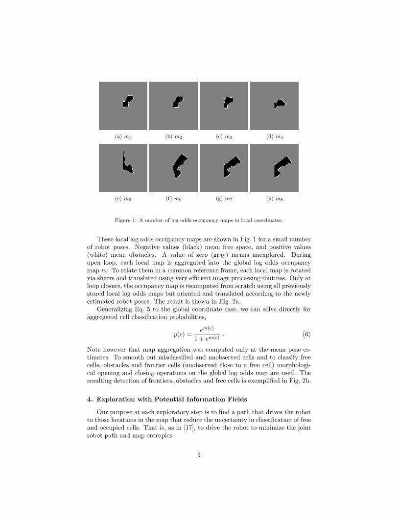
Figure 1: A number of log odds occupancy maps in local coordinates.

These local log odds occupancy maps are shown in Fig. 1 for a small numberof robot poses. Negative values (black) mean free space, and positive values(white) mean obstacles. A value of zero (gray) means unexplored. Duringopen loop, each local map is aggregated into the global log odds occupancymap m. To relate them in a common reference frame, each local map is rotatedvia sheers and translated using very efficient image processing routines. Only atloop closure, the occupancy map is recomputed from scratch using all previouslystored local log odds maps but oriented and translated according to the newlyestimated robot poses. The result is shown in Fig. 2a.

Generalizing Eq. 5 to the global coordinate case, we can solve directly foraggregated cell classification probabilities,

p(c) =em(c)

1 + em(c). (6)

Note however that map aggregation was computed only at the mean pose es-timates. To smooth out misclassified and unobserved cells and to classify freecells, obstacles and frontier cells (unobserved close to a free cell) morphologi-cal opening and closing operations on the global log odds map are used. Theresulting detection of frontiers, obstacles and free cells is exemplified in Fig. 2b.

4. Exploration with Potential Information Fields

Our purpose at each exploratory step is to find a path that drives the robotto those locations in the map that reduce the uncertainty in classification of freeand occupied cells. That is, as in [17], to drive the robot to minimize the jointrobot path and map entropies.

5

(a) (b)

Figure 2: (a) Aggregated log odds occupancy map m. (b) Classified frontier cells (white),obstacle cells (black), free cells (light grey) and unobserved cells (dark grey).

The objective is to find a scalar function φ(c) defined over all C-space cellssuch that its gradient ∇φ will consist of a path with largest joint path and mapentropy decrease. Unfortunately, the entropy decrease when executing a trajec-tory from the current pose to any given C-space configuration is not independentof the path taken to arrive to such pose. Different routes induce different de-crease values of path and map entropies. Take for instance two different routesto the same pose, one that goes close to previously visited locations or one thatdiscovers unexplored areas. In the former, the robot would be able to closeloops, and thus maintain bounded localization uncertainty. In the second, anexploratory route would reduce the map entropy instead.

Computing the optimal path to a goal taking into account the effect on thereduction of joint path and map entropies for each possible route is a computa-tionally intractable process for anything else than very small academic scenar-ios. We are content with obtaining a suboptimal solution, assuming that therobot can reach each possible configuration in one single step and letting PoseSLAM take into account uncertainty reduction during path execution. Thatis, we do consider path and map entropy changes thru the path to each robotconfiguration but only the changes induced in entropy by ’appearing’ at thatconfiguration.

This is a strong assumption since we give up knowing about the change inentropy at intermediate steps for the ability to compute a dense entropy estimateover the whole C-space. This dense estimate ends up being conservative, butthis is not a problem since it is only used for path planning and not to guaranteepath execution. Any event triggering replaning (reaching a goal or a collision)triggers also a new evaluation of the entropy decrease estimate for the wholeC-space. Contrary, in Active Pose SLAM [17], entropy reduction is indeed

6

a b

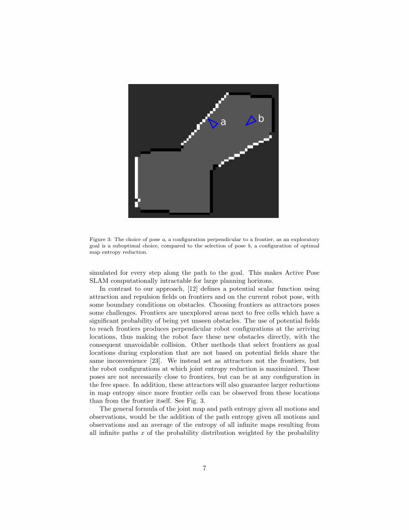
Figure 3: The choice of pose a, a configuration perpendicular to a frontier, as an exploratorygoal is a suboptimal choice, compared to the selection of pose b, a configuration of optimalmap entropy reduction.

simulated for every step along the path to the goal. This makes Active PoseSLAM computationally intractable for large planning horizons.

In contrast to our approach, [12] defines a potential scalar function usingattraction and repulsion fields on frontiers and on the current robot pose, withsome boundary conditions on obstacles. Choosing frontiers as attractors posessome challenges. Frontiers are unexplored areas next to free cells which have asignificant probability of being yet unseen obstacles. The use of potential fieldsto reach frontiers produces perpendicular robot configurations at the arrivinglocations, thus making the robot face these new obstacles directly, with theconsequent unavoidable collision. Other methods that select frontiers as goallocations during exploration that are not based on potential fields share thesame inconvenience [23]. We instead set as attractors not the frontiers, butthe robot configurations at which joint entropy reduction is maximized. Theseposes are not necessarily close to frontiers, but can be at any configuration inthe free space. In addition, these attractors will also guarantee larger reductionsin map entropy since more frontier cells can be observed from these locationsthan from the frontier itself. See Fig. 3.

The general formula of the joint map and path entropy given all motions andobservations, would be the addition of the path entropy given all motions andobservations and an average of the entropy of all infinite maps resulting fromall infinite paths x of the probability distribution weighted by the probability

7

of each possible trajectory:

H(x,m|u, z) = H(x|u, z) +

∫x

p(x|u, z)H(m|x, u, z)dx. (7)

The joint state entropy is approximated, in a similar way as in [17] as

H(x,m|u, z) ≈ H(x|u, z) + α(p(x|u, z))H(m|µx, u, z) (8)

where instead of computing the map entropy averaging for all infinite possiblemaps, we compute it only for the mean pose estimates µx and differently to theapproximation used in [17], we add a factor α(p(x|u, z)) multiplying the mapentropy depending on the probability distribution. Finally, we actually do notwant the absolute value of the joint entropy but its change, so what we need tocompute is

∆H(x,m|u, z) ≈ ∆H(x|u, z) + α(p(x|u, z))∆H(m|µx, u, z). (9)

We evaluate joint entropy reduction on these two terms separately for eachdiscretized robot configuration in C-space, treat this entropy reduction as aninformation field and smooth it to avoid discontinuities. We finally compute theexploration path as the gradient of this field.

4.1. Path entropy reduction

The first term in Eq. 8 accounts for the path entropy, which in Pose SLAMis given by

H(x|u, z) = ln((2πe)(n/2)|Σ|). (10)

The evaluation of Eq. 10 poses some drawbacks. As noted in [13], it can easilybecome ill defined. To overcome this situation one might approximate its valuewithout taking into account the correlation between poses, and averaging overthe individual pose marginals as proposed by Stachniss et al. [15] and alsoimplemented in [17].

This is not necessary in our case, since we are not interested in computingthe entropy itself, but its change –the information gain– (eq. 9) and not for justone posterior pose, but for the whole discretized C-space. To approximate it,we assume a noise free platform for the evaluation of the final leg in the path,and thus the jump from the current pose to each configuration will produce thesame marginal posterior, with zero information gain, except at loop closure.

And, in closing a loop between any previous configuration i and the currentone k, the decrease in path entropy is given precisely by the information gainIik encoded in a link connecting the two nodes as defined in Eq. 3,

∆H(x|u, z) =

{Iik if a loop with configuration i can be closed,0 otherwise

(11)

To establish such a link, the two configurations must be within the sensorrange, i.e., inside the sensor match area. Instead of iterating over each cell in

8

the C-space grid and searching for its loop closure candidates in the Pose SLAMgraph, the iteration proceeds the other way. For each pose in the Pose SLAMgraph, we annotate the cells inside their match area in a C-space path entropydecrease grid with the corresponding information gain. The resulting C-spacegrid contains the amount of path entropy decrease when the robot is moved tothat particular position and orientation.

4.2. Map entropy reduction

In contrast to [17], in which we compute the reduction in entropy for alimited set of final configurations, we now compute it for each configuration inthe discretized C-space. For a map with size cell l, its entropy can be computedas a scalar value

H(m|u, z) = −l2∑∀c∈m

(p(c) log p(c) + (1− p(c)) log(1− p(c))). (12)

The reduction in entropy that is attained after moving to a new locationand sensing new data depends basically on the number of cells that will changeits status from unknown to discovered, either obstacle or free. Anticipating thenumber of discovered free cells before actually processing the new observationsis impossible. We are content with approximating entropy reduction as theincrease in the number of discovered frontier cells.

This map entropy reduction by observing frontier cells for each robot con-figuration could be found computing the frontier visibility of each sensor rayfor each robot configurations but this wouldn’t be efficient at all. We proposeinstead a novel method for computing it efficiently using convolutions. Takinginto account that several robot orientations have common ray directions, andalso that using a simple convolution, we can compute the frontier visibility fora specific direction from all positions, we invert the order of computations.

Hence, we are able to compute this entropy change very efficiently with thefollowing three steps:

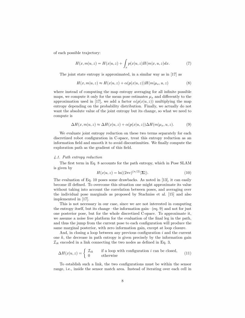
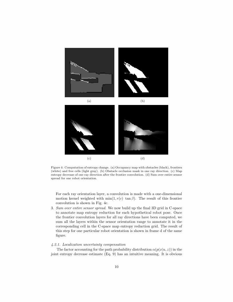
1. Obstacle occlusion mask. We generate a three-dimensional grid. Its dimen-sions are x, y, and the orientation of each laser ray. For each ray orientationlayer, a 2D obstacle occlusion mask is created, annotating whether the near-est non-free cell along that ray direction is a frontier or not. The mask iscomputed with a one-dimensional convolution with an inverse exponentialmotion kernel over a positive value for frontier cells and a negative valuefor obstacles. Binary thresholding the positive values we obtain the desiredocclusion mask. See Fig. 4b.

2. Frontier convolution. Given the radial nature of the sensor being simulated,each frontier cell will receive a different density of ray casts from the samescan, thus it is necessary to compensate for this in order not to overestimatethe number of frontier cells being observed. The ray cast density n(c) at eachcell c is modeled as a function of the distance from the robot to that cell r(c)and the angle β between two consecutive sensor rays

n(c) =1

r(c) tanβ. (13)

9

(a) (b)

(c) (d)

Figure 4: Computation of entropy change. (a) Occupancy map with obstacles (black), frontiers(white) and free cells (light gray). (b) Obstacle occlusion mask in one ray direction. (c) Mapentropy decrease of one ray direction after the frontier convolution. (d) Sum over entire sensorspread for one robot orientation.

For each ray orientation layer, a convolution is made with a one-dimensionalmotion kernel weighted with min(1, r(c) tanβ). The result of this frontierconvolution is shown in Fig. 4c.

3. Sum over entire sensor spread. We now build up the final 3D grid in C-spaceto annotate map entropy reduction for each hypothetical robot pose. Oncethe frontier convolution layers for all ray directions have been computed, wesum all the layers within the sensor orientation range to annotate it in thecorresponding cell in the C-space map entropy reduction grid. The result ofthis step for one particular robot orientation is shown in frame d of the samefigure.

4.2.1. Localization uncertainty compensation

The factor accounting for the path probability distribution α(p(x|u, z)) in thejoint entropy decrease estimate (Eq. 9) has an intuitive meaning. It is obvious

10

that exploratory trajectories that depart from well localized priors produce moreaccurate maps than explorations that depart from uncertain locations. In fact,sensor readings coming from robot poses with large marginal covariance valuesmay spoil the map adding bad cell classifications, i.e., adding entropy. Sincewe already have localization uncertainties encoded in the Pose SLAM graph,these are used to weight the entire entropy reduction map. It suffices to weightthe entire entropy reduction map with the inverse of the determinant of themarginal covariance at the current configuration

α(p(x|u, z)) =1

|Σkk|(14)

Exploratory trajectories that depart from uncertain configurations will beweighted negatively, giving predominance to the path entropy reduction termin those cases. In this way, we achieve the desired effect of alternance betweenexploratory and relocalization paths.

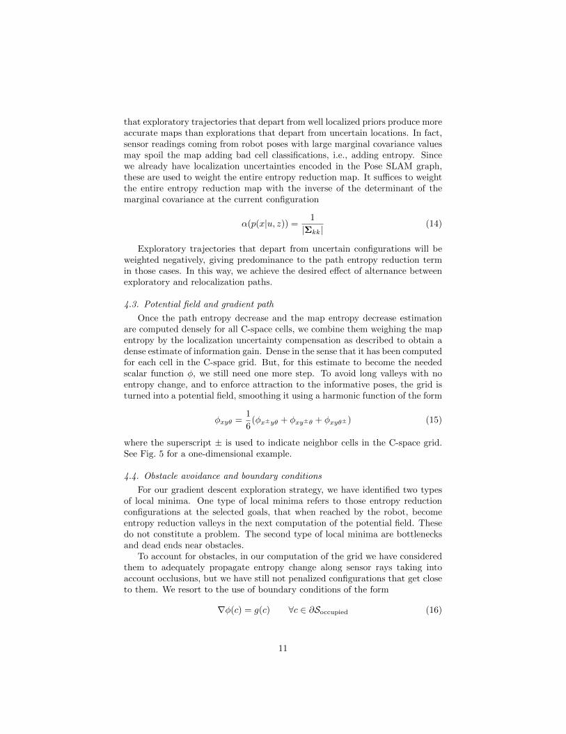
4.3. Potential field and gradient path

Once the path entropy decrease and the map entropy decrease estimationare computed densely for all C-space cells, we combine them weighing the mapentropy by the localization uncertainty compensation as described to obtain adense estimate of information gain. Dense in the sense that it has been computedfor each cell in the C-space grid. But, for this estimate to become the neededscalar function φ, we still need one more step. To avoid long valleys with noentropy change, and to enforce attraction to the informative poses, the grid isturned into a potential field, smoothing it using a harmonic function of the form

φxyθ =1

6(φx±yθ + φxy±θ + φxyθ±) (15)

where the superscript ± is used to indicate neighbor cells in the C-space grid.See Fig. 5 for a one-dimensional example.

4.4. Obstacle avoidance and boundary conditions

For our gradient descent exploration strategy, we have identified two typesof local minima. One type of local minima refers to those entropy reductionconfigurations at the selected goals, that when reached by the robot, becomeentropy reduction valleys in the next computation of the potential field. Thesedo not constitute a problem. The second type of local minima are bottlenecksand dead ends near obstacles.

To account for obstacles, in our computation of the grid we have consideredthem to adequately propagate entropy change along sensor rays taking intoaccount occlusions, but we have still not penalized configurations that get closeto them. We resort to the use of boundary conditions of the form

∇φ(c) = g(c) ∀c ∈ ∂Soccupied (16)

11

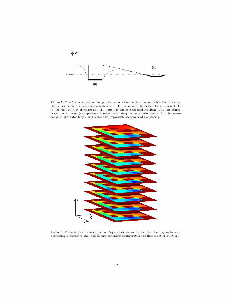
Figure 5: The C-space entropy change grid is smoothed with a harmonic function updatingthe values below v at each smooth iteration. The solid and the dotted lines represent theinitial joint entropy decrease and the potential information field resulting after smoothing,respectively. Zone (a) represents a region with steep entropy reduction within the sensorrange to guarantee loop closure. Zone (b) represents an area worth exploring.

Figure 6: Potential field values for some C-space orientation layers. The blue regions indicatecompeting exploratory and loop closure candidate configurations at that robot orientation.

12

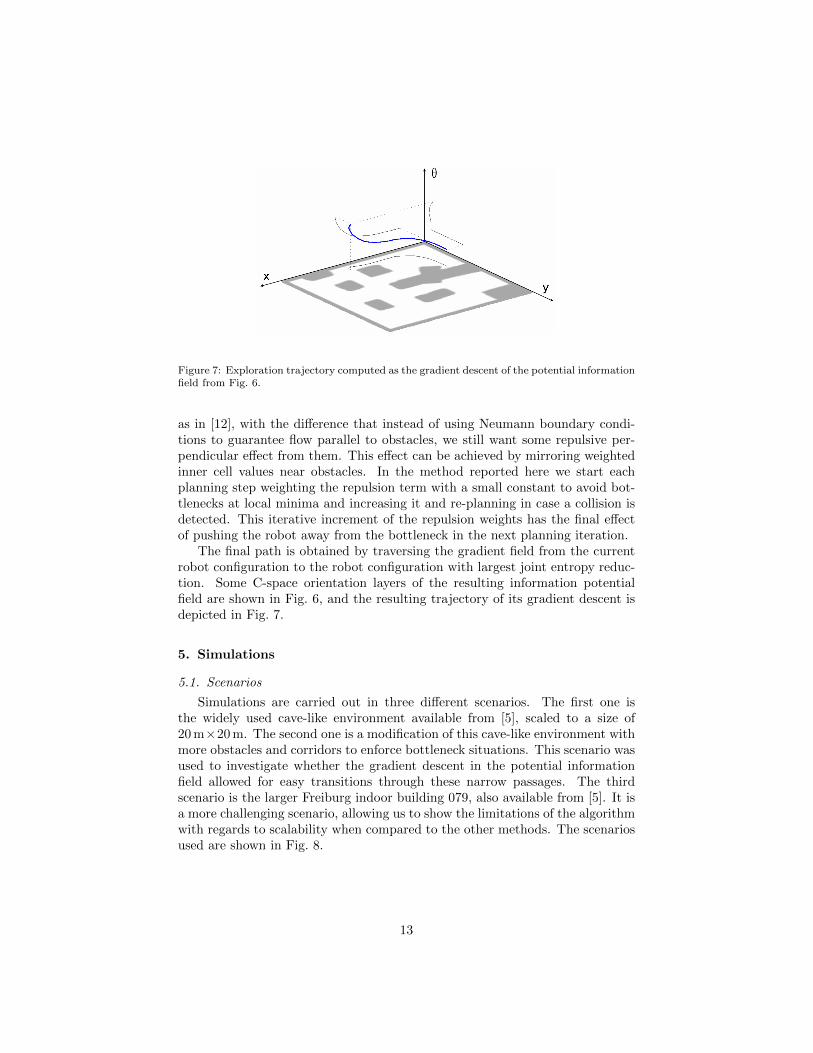
Figure 7: Exploration trajectory computed as the gradient descent of the potential informationfield from Fig. 6.

as in [12], with the difference that instead of using Neumann boundary condi-tions to guarantee flow parallel to obstacles, we still want some repulsive per-pendicular effect from them. This effect can be achieved by mirroring weightedinner cell values near obstacles. In the method reported here we start eachplanning step weighting the repulsion term with a small constant to avoid bot-tlenecks at local minima and increasing it and re-planning in case a collision isdetected. This iterative increment of the repulsion weights has the final effectof pushing the robot away from the bottleneck in the next planning iteration.

The final path is obtained by traversing the gradient field from the currentrobot configuration to the robot configuration with largest joint entropy reduc-tion. Some C-space orientation layers of the resulting information potentialfield are shown in Fig. 6, and the resulting trajectory of its gradient descent isdepicted in Fig. 7.

5. Simulations

5.1. Scenarios

Simulations are carried out in three different scenarios. The first one isthe widely used cave-like environment available from [5], scaled to a size of20 m×20 m. The second one is a modification of this cave-like environment withmore obstacles and corridors to enforce bottleneck situations. This scenario wasused to investigate whether the gradient descent in the potential informationfield allowed for easy transitions through these narrow passages. The thirdscenario is the larger Freiburg indoor building 079, also available from [5]. It isa more challenging scenario, allowing us to show the limitations of the algorithmwith regards to scalability when compared to the other methods. The scenariosused are shown in Fig. 8.

13

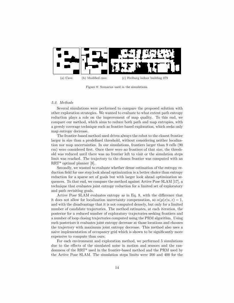
(a) Cave (b) Modified cave (c) Freiburg indoor building 079

Figure 8: Scenarios used in the simulations.

5.2. Methods

Several simulations were performed to compare the proposed solution withother exploration strategies. We wanted to evaluate to what extent path entropyreduction plays a role on the improvement of map quality. To this end, wecompare our method, which aims to reduce both path and map entropies, witha greedy coverage technique such as frontier-based exploration, which seeks onlymap entropy decrease.

The frontier-based method used drives always the robot to the closest frontierlarger in size than a predefined threshold, without considering neither localiza-tion nor map uncertainties. In our simulations, frontiers larger than 9 cells (90cm) were considered first. Once there were no frontiers of that size, the thresh-old was reduced until there was no frontier left to visit or the simulation stepslimit was reached. The trajectory to the chosen frontier was computed with anRRT* optimal planner [8].

Secondly, we wanted to evaluate whether dense estimation of the entropy re-duction field for one step look ahead optimization is a better choice than entropyreduction for a sparse set of goals but with larger look ahead optimization se-quences. To that end, we compare the method against Active Pose SLAM [17], atechnique that evaluates joint entropy reduction for a limited set of exploratoryand path revisiting goals.

Active Pose SLAM evaluates entropy as in Eq. 8, with the difference thatit does not allow for localization uncertainty compensation, so α(p(x|u, z) = 1,and with the disadvantage that it is not computed densely, but only for a limitednumber of candidate trajectories. The method estimates, at each iteration, theposterior for a reduced number of exploratory trajectories seeking frontiers anda number of loop closing trajectories computed using the PRM algorithm. Usingsuch posteriors it evaluates joint entropy decrease at those locations and choosesthe trajectory with maximum joint entropy decrease. This method also uses anaive implementation of occupancy grid which is shown to be significantly moreexpensive to compute than ours.

For each environment and exploration method, we performed 5 simulationsdue to the effects of the simulated noise in motion and sensors and the ran-domness of the RRT* used in the frontier-based method and the PRM used bythe Active Pose SLAM. The simulation steps limits were 200 and 400 for the

14

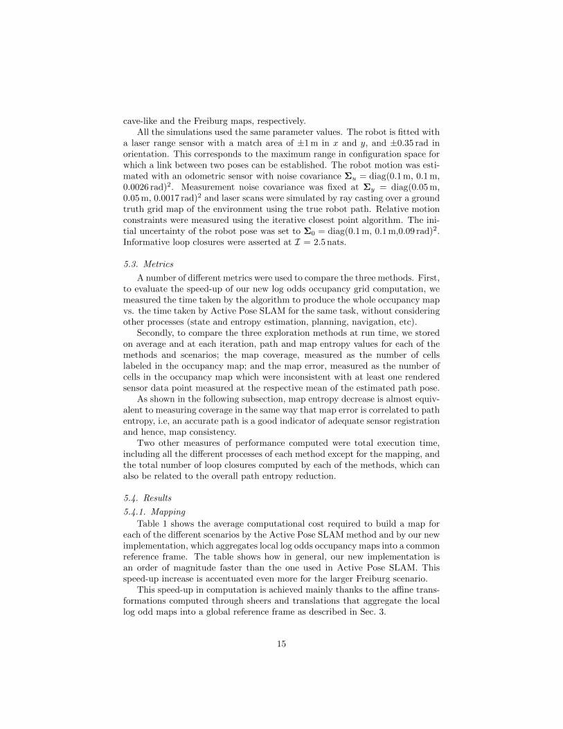
cave-like and the Freiburg maps, respectively.All the simulations used the same parameter values. The robot is fitted with

a laser range sensor with a match area of ±1 m in x and y, and ±0.35 rad inorientation. This corresponds to the maximum range in configuration space forwhich a link between two poses can be established. The robot motion was esti-mated with an odometric sensor with noise covariance Σu = diag(0.1 m, 0.1 m,0.0026 rad)2. Measurement noise covariance was fixed at Σy = diag(0.05 m,0.05 m, 0.0017 rad)2 and laser scans were simulated by ray casting over a groundtruth grid map of the environment using the true robot path. Relative motionconstraints were measured using the iterative closest point algorithm. The ini-tial uncertainty of the robot pose was set to Σ0 = diag(0.1 m, 0.1 m,0.09 rad)2.Informative loop closures were asserted at I = 2.5 nats.

5.3. Metrics

A number of different metrics were used to compare the three methods. First,to evaluate the speed-up of our new log odds occupancy grid computation, wemeasured the time taken by the algorithm to produce the whole occupancy mapvs. the time taken by Active Pose SLAM for the same task, without consideringother processes (state and entropy estimation, planning, navigation, etc).

Secondly, to compare the three exploration methods at run time, we storedon average and at each iteration, path and map entropy values for each of themethods and scenarios; the map coverage, measured as the number of cellslabeled in the occupancy map; and the map error, measured as the number ofcells in the occupancy map which were inconsistent with at least one renderedsensor data point measured at the respective mean of the estimated path pose.

As shown in the following subsection, map entropy decrease is almost equiv-alent to measuring coverage in the same way that map error is correlated to pathentropy, i.e, an accurate path is a good indicator of adequate sensor registrationand hence, map consistency.

Two other measures of performance computed were total execution time,including all the different processes of each method except for the mapping, andthe total number of loop closures computed by each of the methods, which canalso be related to the overall path entropy reduction.

5.4. Results

5.4.1. Mapping

Table 1 shows the average computational cost required to build a map foreach of the different scenarios by the Active Pose SLAM method and by our newimplementation, which aggregates local log odds occupancy maps into a commonreference frame. The table shows how in general, our new implementation isan order of magnitude faster than the one used in Active Pose SLAM. Thisspeed-up increase is accentuated even more for the larger Freiburg scenario.

This speed-up in computation is achieved mainly thanks to the affine trans-formations computed through sheers and translations that aggregate the locallog odd maps into a global reference frame as described in Sec. 3.

15

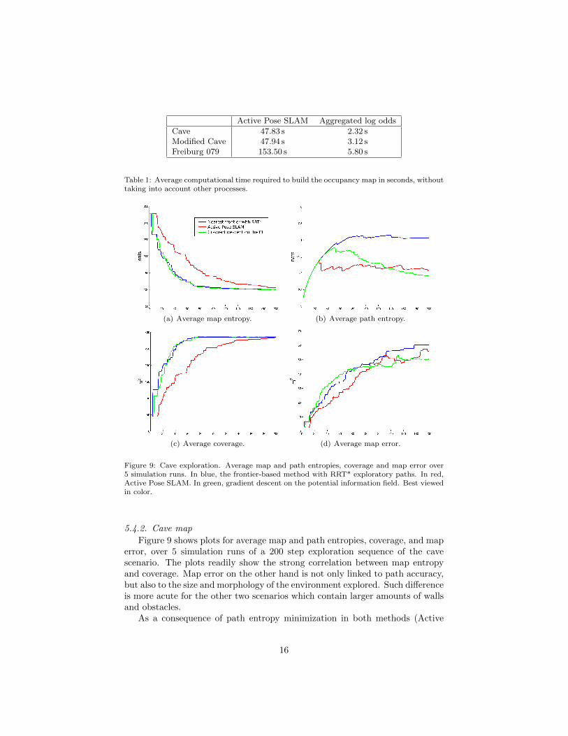
Active Pose SLAM Aggregated log odds

Cave 47.83 s 2.32 sModified Cave 47.94 s 3.12 sFreiburg 079 153.50 s 5.80 s

Table 1: Average computational time required to build the occupancy map in seconds, withouttaking into account other processes.

(a) Average map entropy. (b) Average path entropy.

(c) Average coverage. (d) Average map error.

Figure 9: Cave exploration. Average map and path entropies, coverage and map error over5 simulation runs. In blue, the frontier-based method with RRT* exploratory paths. In red,Active Pose SLAM. In green, gradient descent on the potential information field. Best viewedin color.

5.4.2. Cave map

Figure 9 shows plots for average map and path entropies, coverage, and maperror, over 5 simulation runs of a 200 step exploration sequence of the cavescenario. The plots readily show the strong correlation between map entropyand coverage. Map error on the other hand is not only linked to path accuracy,but also to the size and morphology of the environment explored. Such differenceis more acute for the other two scenarios which contain larger amounts of wallsand obstacles.

As a consequence of path entropy minimization in both methods (Active

16

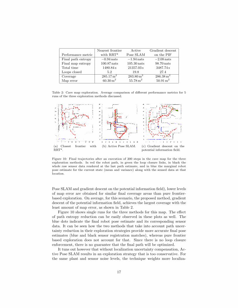
Nearest frontier Active Gradient descentPerformance metric with RRT* Pose SLAM on the PIF

Final path entropy −0.94 nats −1.94 nats −2.08 natsFinal map entropy 100.87 nats 105.30 nats 98.70 natsTotal time 1480.84 s 21357.03 s 3487.74 sLoops closed 5.2 19.8 27.4

Coverage 285.17 m2 283.80 m2 286.38 m2

Map error 60.30 m2 55.78 m2 50.91 m2

Table 2: Cave map exploration. Average comparison of different performance metrics for 5runs of the three exploration methods discussed.

(a) Closest frontier withRRT*.

(b) Active Pose SLAM. (c) Gradient descent on thepotential information field.

Figure 10: Final trajectories after an execution of 200 steps in the cave map for the threeexploration methods. In red the robot path, in green the loop closure links, in black thewhole raw sensor data rendered at the last path estimate, and in blue the marginal robotpose estimate for the current state (mean and variance) along with the sensed data at thatlocation.

Pose SLAM and gradient descent on the potential information field), lower levelsof map error are obtained for similar final coverage areas than pure frontier-based exploration. On average, for this scenario, the proposed method, gradientdescent of the potential information field, achieves the largest coverage with theleast amount of map error, as shown in Table 2.

Figure 10 shows single runs for the three methods for this map. The effectof path entropy reduction can be easily observed in these plots as well. Theblue dots indicate the final robot pose estimate and its corresponding sensordata. It can be seen how the two methods that take into account path uncer-tainty reduction in their exploration strategies provide more accurate final poseestimates (blue and black sensor registration matches), whereas pure frontierbased exploration does not account for that. Since there is no loop closureenforcement, there is no guarantee that the final path will be optimized.

It tuns out however that without localization uncertainty compensation, Ac-tive Pose SLAM results in an exploration strategy that is too conservative. Forthe same plant and sensor noise levels, the technique weights more localiza-

17

tion than exploration and hence coverage grows slower than in the other twomethods.

Our method outperforms both other methods reaching full coverage muchfaster, and with lower path entropy. In addition, the computational time for theaggregated exploration and planning routines is significantly lower than ActivePose SLAM and competitive with the frontier-based method.

In the figure, it can also be observed how the frontier-based strategy re-sults in many collisions with many frontiers misclassified due to the larger pathuncertainties. In contrast, the exploration method using the gradient descenton the potential information field produces valleys of high information at loopclosures and away from the repulsive obstacles.

Another difference between the two methods is that frontier-based explo-ration ceases once full coverage is reached and there are no further frontiers tovisit. On the contrary, our method even when reaching full coverage, mightcontinue optimizing the path, seeking revisiting trajectories to close loops, andhence improving the map estimate.

5.4.3. Modified cave map

This second scenario is a modification of the cave map in which we haveadded walls and obstacles to create a more challenging environment. The ob-jective in designing this setting was to analyze whether the gradient descentapproach would get stuck in local minima at corridors or dead ends.

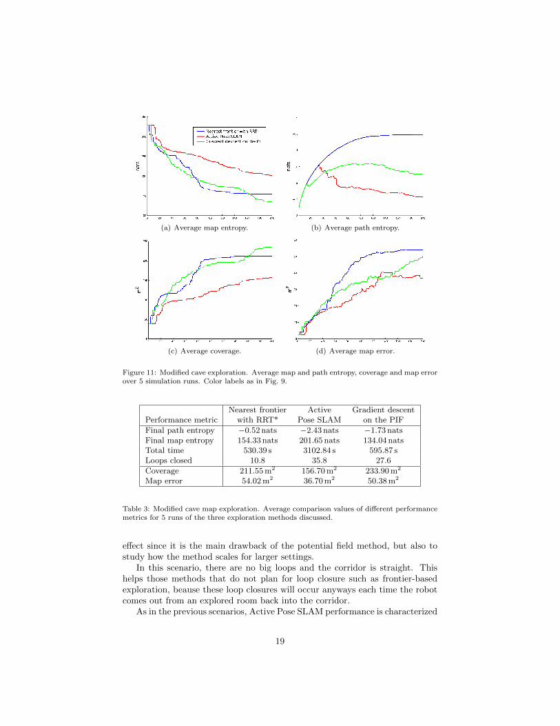
Figure 11 shows once more averaged metrics for the three methods in thisscenario for five simulation runs. One interesting thing to note is that frontier-based exploration rapidly enforces coverage, reaching low map entropy valuessooner than the other methods, but being unable to decrease such value at theend of the simulation. The reason for this is that disregarding path entropyminimization in frontier-based does not enforce loop closure. For that samereason frontier-based exploration produced the largest map errors. The two jointentropy minimization schemes performed reasonably well with regards to pathentropy reduction. However, our method was more conservative in explorationat the beginning, reaching better coverage at the end, whereas Active PoseSLAM was too conservative heavily refining its localization estimates for thisscenario and failed to fully explore it.

These same findings are also contrasted in Table 3 and in the exemplarytest runs plotted in Fig. 12. See for instance the large number of collisions thatneeded to be accounted for in the frontier-based method due to its larger maperror values.

Computationally speaking, our gradient descent takes similar effort to com-pute than frontier-based exploration, and is about six times faster than ActivePose SLAM on average for this scenario.

5.5. Freiburg 079 map

The Freigurg 079 building is quite more complex than the two previousscenarios. We choose this environment in order to test not only the bottleneck

18


(c) Average coverage. (d) Average map error.

Figure 11: Modified cave exploration. Average map and path entropy, coverage and map errorover 5 simulation runs. Color labels as in Fig. 9.



Coverage 211.55 m2 156.70 m2 233.90 m2

Map error 54.02 m2 36.70 m2 50.38 m2

Table 3: Modified cave map exploration. Average comparison values of different performancemetrics for 5 runs of the three exploration methods discussed.

effect since it is the main drawback of the potential field method, but also tostudy how the method scales for larger settings.

In this scenario, there are no big loops and the corridor is straight. Thishelps those methods that do not plan for loop closure such as frontier-basedexploration, beause these loop closures will occur anyways each time the robotcomes out from an explored room back into the corridor.

As in the previous scenarios, Active Pose SLAM performance is characterized

19

(a) Nearest frontier withRRT*.

(b) Active Pose SLAM. (c) Gradient descent on thepotential information field.

Figure 12: Final trajectories after an execution of 200 steps in the modified cave map of thethree exploration methods. Color meanings as in Fig. 10.

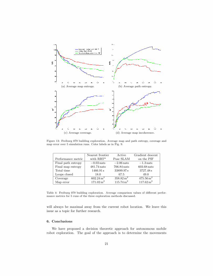
by a very conservative behavior with regards to localization uncertainty. Fora simulation run of 400 steps, the method did not reach full coverage. Theresult was a largely connected graph of nodes around the initial robot pose,with very low path entropy, leaving the rest of the scene highly unexplored.As expected, the closest frontier method behaves the opposite way, it reachesnearly full coverage and, due to the topology of the scenario, closes a significantnumber of loops. Path entropy and map error however are still larger than inthe other two methods.

Our method shows a more balanced performance with regards to explorationvs. exploitation, as shown in Fig. 14 which plots the resulting map for one in-stance of the simulations after 400 steps for each of the three methods discussed.

For the potential information fields method, the local minima drawback isdetected in two different cases, as a bottleneck effect near obstacles and also aslocal minima of path entropy. The first case is mainly a planning drawback,narrow door passages tend to trap the robot because of the repulsive boundaryconditions at obstacles. To get away from these local minima, it sufficed toincrease the potential field at that node, turning a valley into a ridge. Thisiterative potential field increase constituted a two-fold increase in computationtime when compared with the frontier-based method, as shown in Table 4.

The second case of local minima appears in the second half of the simulation.At that point marginal pose uncertainties have become large enough to populatethe Pose SLAM graph with plenty of nearby nodes. A gradient descent pathwill seek loop closure with such nodes but with little path entropy reduction.Navigating around these nearly flat potential fields will not significantly reducemap entropy either, but will introduce motion and sensor error, hence producingmap error in the end as shown in Fig. 13. The end result is that for the secondhalf of the simulation, coverage does not increase as fast as in the first part. Apossible solution to this problem would be to change our state representation tolocal coordinates instead of global. In that case, marginals close to the currentrobot location would always have smaller variance, and path entropy reduction

20


(c) Average coverage. (d) Average map incoherence.

Figure 13: Freiburg 079 building exploration. Average map and path entropy, coverage andmap error over 5 simulation runs. Color labels as in Fig. 9.



Coverage 602.24 m2 358.82 m2 475.56 m2

Map error 171.02 m2 115.74 m2 117.62 m2

Table 4: Freiburg 079 building exploration. Average comparison values of different perfor-mance metrics for 5 runs of the three exploration methods discussed.

will always be maximal away from the current robot location. We leave thisissue as a topic for further research.

6. Conclusions

We have proposed a decision theoretic approach for autonomous mobilerobot exploration. The goal of the approach is to determine the movements

21

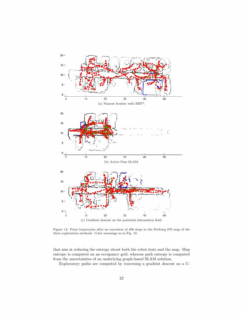
(a) Nearest frontier with RRT*.

(b) Active Pose SLAM.

(c) Gradient descent on the potential information field.

Figure 14: Final trajectories after an execution of 400 steps in the Freiburg 079 map of thethree exploration methods. Color meanings as in Fig. 10.

that aim at reducing the entropy about both the robot state and the map. Mapentropy is computed on an occupancy grid, whereas path entropy is computedfrom the uncertainties of an underlying graph-based SLAM solution.

Exploratory paths are computed by traversing a gradient descent on a C-

22

space field of path and map entropy reduction estimates. The technique makesuse of very efficient convolutions first, to project boundaries along sensor rays,and secondly, to integrate entropy measures at independent robot orientationlayers.

The method outperforms, in terms of map quality, frontier-based explorationwhich only seek coverage. The method also outperforms another method thatseeks joint path and map entropy minimization but only for a limited numberof exploratory trajectories. In this case, both in terms of coverage and speed ofcomputation.

Contrary to other exploration methods, joint path and map entropy decreaseis computed densely over the C-space. In computing the gradient descent onthis field, the method assumes an holonomic platform. Also, the use of thegradient descent makes the method sensitive to some local minima drawbacks.Future work is on using this dense joint entropy decrease estimation to computepotential exploratory goals, but leaving the path planning strategies to othermethods that can account for the non-holonomic restrictions and also be lesssensitive to this local minima [19].

Future work also includes, the switch from global to local representations,an implementation in ROS, and comparison against competing approaches onreal scenarios.

References

[1] F. Bourgault, A.A. Makarenko, S.B. Williams, B. Grocholsky, and H.F.Durrant-Whyte. Information based adaptative robotic exploration. In Proc.IEEE/RSJ Int. Conf. Intell. Robots Syst., pages 540–545, Lausanne, Oct.2002.

[2] E.P. de Silva, P.M. Engel, M. Trevisan, and M.A.P. Idiart. Explorationmethod using harmonic functions. Robotics Auton. Syst., 51(1):25 – 42,2002.

[3] R. M. Eustice, H. Singh, and J. J. Leonard. Exactly sparse delayed-statefilters for view-based SLAM. IEEE Trans. Robotics, 22(6):1100–1114, Dec.2006.

[4] H. J. S. Feder, J. J. Leonard, and C. M. Smith. Adaptive mobile robotnavigation and mapping. Int. J. Robotics Res., 18:650–668, 1999.

[5] A. Howard and N. Roy. The robotics data set repository (Radish).http://radish.sourceforge.net, 2003.

[6] S. Huang, N.M. Kwok, G. Dissanayake, Q.P. Ha, and G. Fang. Multi-steplook-ahead trajectory planning in SLAM: Possibility and necessity. In Proc.IEEE Int. Conf. Robotics Autom., pages 1091–1096, Barcelona, Apr. 2005.

[7] V. Ila, J. M. Porta, and J. Andrade-Cetto. Information-based compactPose SLAM. IEEE Trans. Robotics, 26(1):78–93, Feb. 2010.

23

[8] S. Karaman, M.R. Walter, A. Perez, E. Frazzoli, and S. Teller. Anytimemotion planning using the RRT*. In Proc. IEEE Int. Conf. Robotics Au-tom., pages 1478–1483, Shanghai, May 2011.

[9] A. Kim and R. M. Eustice. Perception-driven navigation: Active visualSLAM for robotic area coverage. In Proc. IEEE Int. Conf. Robotics Autom.,pages 3196–3203, Karlsruhe, May 2013.

[10] C. Leung, S. Huang, and G. Dissanayake. Active SLAM for structuredenvironments. In IEEE Int. Conf. Robotics Autom., pages 1898–1903,Pasadena, 2008.

[11] C. Leung, S. Huang, N. Kwok, and G. Dissanayake. Planning under uncer-tainty using model predictive control for information gathering. RoboticsAuton. Syst., 54(11):898–910, Nov. 2006.

[12] R. Shade and P. Newman. Choosing where to go: Complete 3D explorationwith stereo. In Proc. IEEE Int. Conf. Robotics Autom., pages 2806–2811,Shanghai, May 2011.

[13] R. Sim and N. Roy. Global A-optimal robot exploration in SLAM. In Proc.IEEE Int. Conf. Robotics Autom., pages 661–666, Barcelona, Apr. 2005.

[14] R. C. Smith and P. Cheeseman. On the representation and estimation ofspatial uncertainty. Int. J. Robotics Res., 5(4):56–68, 1986.

[15] C. Stachniss, G. Grisetti, and W. Burgard. Information gain-based explo-ration using Rao-Blackwellized particle filters. In Robotics: Science andSystems I, pages 65–72, Cambridge, Jun. 2005.

[16] R. Valencia, M. Morta, J. Andrade-Cetto, and J.M. Porta. Planning reliablepaths with Pose SLAM. IEEE Trans. Robotics, 29(4):1050–1059, 2013.

[17] R. Valencia, J. Valls Miro, G. Dissanayake, and J. Andrade-Cetto. ActivePose SLAM. In Proc. IEEE/RSJ Int. Conf. Intell. Robots Syst., pages1885–1891, Vilamoura, Oct. 2012.

[18] J. Vallve and J. Andrade-Cetto. Mobile robot exploration with poten-tial information fields. In Proc. Eur. Conf. Mobile Robots, pages 222–227,Barcelona, Sep. 2013.

[19] J. Vallve and J. Andrade-Cetto. Dense entropy decrease estimation formobile robot exploration. In Proc. IEEE Int. Conf. Robotics Autom., pages6083–6089, Hong Kong, May 2014.

[20] T. Vidal-Calleja, A. Sanfeliu, and J. Andrade-Cetto. Action selection forsingle camera SLAM. IEEE Trans. Syst., Man, Cybern. B, 40(6):1567–1581, Dec. 2010.

[21] P. Whaite and F. P. Ferrie. Autonomous exploration: Driven by uncer-tainty. IEEE Trans. Pattern Anal. Mach. Intell., 19(3):193–205, Mar. 1997.

24

[22] B. Yamauchi. A frontier-based approach for autonomous exploration. InIEEE Int. Sym. Computational Intell. Robot. Automat., pages 146–151,Monterrey, 1997.

[23] B. Yamauchi. Frontier-based exploration using multiple robots. In Int.Conf. Autonomous Agents, pages 47–53, Minneapolis, 1998.

25

potential information fields for mobile robot … · potential information elds for mobile robot...

Documents