potential flows - school of mathematics | university of leedskersale/2620/notes/chapter_4.pdf ·...
TRANSCRIPT

Chapter 4
Potential flows
Contents
4.1 Velocity potential . . . . . . . . . . . . . . . . . . . . . . . . . . . . . 27
4.2 Kinematic boundary conditions . . . . . . . . . . . . . . . . . . . . . 28
4.3 Elementary potential flows . . . . . . . . . . . . . . . . . . . . . . . . 28
4.4 Properties of Laplace’s equation . . . . . . . . . . . . . . . . . . . . 31
4.5 Flow past an obstacle . . . . . . . . . . . . . . . . . . . . . . . . . . . 32
4.6 Method of images . . . . . . . . . . . . . . . . . . . . . . . . . . . . . 35
4.7 Method of separation of variables . . . . . . . . . . . . . . . . . . . . 35
4.1 Velocity potential
We shall now consider the special case of irrotational flows, i.e. flows with no vorticity, suchthat
ω = ∇× u = 0. (4.1)
If a velocity field u is irrotational, that is if ∇× u = 0, then there exists a velocity potential
φ(x, t) defined byu = ∇φ. (4.2)
This is a result from vector calculus; the converse is trivially true since ∀φ, ∇×∇φ ≡ 0.
If in addition the flow is incompressible, the velocity potential φ satisfies Laplace’s equation
∇2φ = 0. (4.3)
Indeed, for incompressible irrotational flows one has ∇ · u = ∇ · ∇φ = ∇2φ = 0.
Hence, incompressible irrotational flows can be computed by solving Laplace’s equation (4.3)and imposing appropriate boundary conditions (or conditions at infinity) on the solution.(Notice that for 2-D incompressible irrotational flows, both velocity potential, φ, and stream-function, ψ, are solutions to Laplace’s equation, ∇2ψ = −ω = 0 and ∇2φ = 0; boundaryconditions on ψ and φ are different however.)
27
28 4.2 Kinematic boundary conditions
4.2 Kinematic boundary conditions
U
n
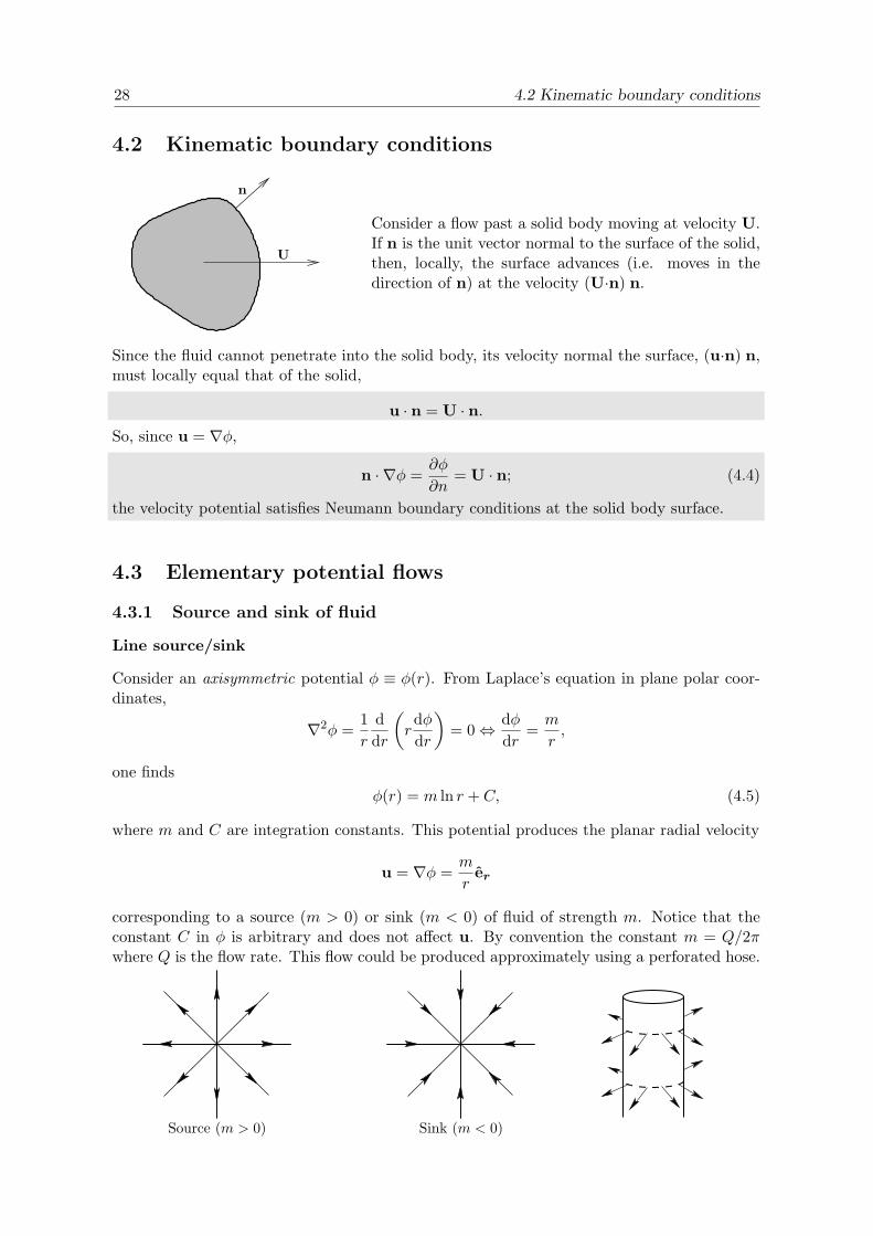
Consider a flow past a solid body moving at velocity U.If n is the unit vector normal to the surface of the solid,then, locally, the surface advances (i.e. moves in thedirection of n) at the velocity (U·n) n.
Since the fluid cannot penetrate into the solid body, its velocity normal the surface, (u·n) n,must locally equal that of the solid,
u · n = U · n.So, since u = ∇φ,
n · ∇φ =∂φ
∂n= U · n; (4.4)
the velocity potential satisfies Neumann boundary conditions at the solid body surface.
4.3 Elementary potential flows
4.3.1 Source and sink of fluid
Line source/sink
Consider an axisymmetric potential φ ≡ φ(r). From Laplace’s equation in plane polar coor-dinates,
∇2φ =1
r
d
dr
(
rdφ
dr
)
= 0 ⇔ dφ
dr=m
r,
one finds
φ(r) = m ln r + C, (4.5)
where m and C are integration constants. This potential produces the planar radial velocity
u = ∇φ =m
rer
corresponding to a source (m > 0) or sink (m < 0) of fluid of strength m. Notice that theconstant C in φ is arbitrary and does not affect u. By convention the constant m = Q/2πwhere Q is the flow rate. This flow could be produced approximately using a perforated hose.
Source (m > 0) Sink (m < 0)

Chapter 4 – Potential flows 29
Point source/sink
Consider a spherically symmetric potential φ ≡ φ(r). From Laplace’s equation in sphericalpolar coordinates,
∇2φ =1
r2d
dr
(
r2dφ
dr
)
= 0 ⇔ dφ
dr=m
r2,
one finds
φ(r) = −mr
+ C, (4.6)
where m and C are integration constants. This potential produces the three-dimensionalradial velocity
u = ∇φ =m
r2er.
corresponding to a source (m > 0) or sink (m < 0) of fluid of strength m. By convention theconstant m = Q/4π where Q is the flow rate or volume flux.
Source (m > 0) Sink (m < 0)
4.3.2 Line vortex
For the potential φ(θ) = kθ, solution to Laplace’s equationin plane polar coordinates, one has
ur =∂φ
∂r= 0 and uθ =
1
r
∂φ
∂θ=k
r,
where the strength of the flow k is a constant. By conventionk = Γ/2π if Γ is the circulation of the flow.This represents a rotating fluid (bath-plug vortex) around a line vortex at r = 0; it has zerovorticity but is singular at the origin.
4.3.3 Uniform stream
For a uniform flow along the z-axis, u = (0, 0, U), the velocity potential
φ(z) = Uz.
(The integration constant is set to zero.)
4.3.4 Dipole (doublet flow)
Since Laplace’s equation is linear we can add two solutions together to form a new one. Adipole is the superposition of a sink and an source of equal but opposite strength next to eachother.
30 4.3 Elementary potential flows
Three-dimensional flow
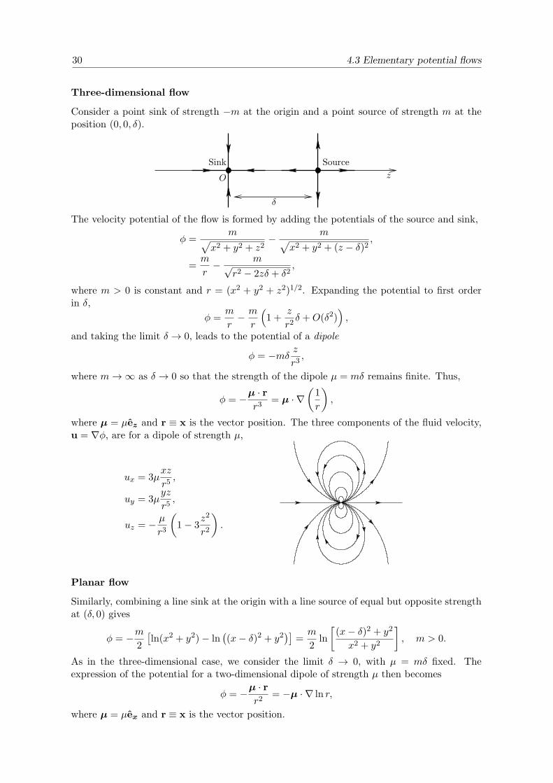
Consider a point sink of strength −m at the origin and a point source of strength m at theposition (0, 0, δ).
z
Sink Source
δ
O
The velocity potential of the flow is formed by adding the potentials of the source and sink,
φ =m
√
x2 + y2 + z2− m√
x2 + y2 + (z − δ)2,
=m
r− m√
r2 − 2zδ + δ2,
where m > 0 is constant and r = (x2 + y2 + z2)1/2. Expanding the potential to first orderin δ,
φ =m
r− m
r
(
1 +z
r2δ +O(δ2)
)
,
and taking the limit δ → 0, leads to the potential of a dipole
φ = −mδ zr3,
where m→ ∞ as δ → 0 so that the strength of the dipole µ = mδ remains finite. Thus,
φ = −µ · rr3
= µ · ∇(
1
r
)
,
where µ = µez and r ≡ x is the vector position. The three components of the fluid velocity,u = ∇φ, are for a dipole of strength µ,
ux = 3µxz
r5,
uy = 3µyz
r5,
uz = − µ
r3
(
1− 3z2
r2
)
.
Planar flow
Similarly, combining a line sink at the origin with a line source of equal but opposite strengthat (δ, 0) gives
φ = −m2
[
ln(x2 + y2)− ln(
(x− δ)2 + y2)]
=m
2ln
[
(x− δ)2 + y2
x2 + y2
]
, m > 0.
As in the three-dimensional case, we consider the limit δ → 0, with µ = mδ fixed. Theexpression of the potential for a two-dimensional dipole of strength µ then becomes
φ = −µ · rr2
= −µ · ∇ ln r,
where µ = µex and r ≡ x is the vector position.
Chapter 4 – Potential flows 31
4.4 Properties of Laplace’s equation
4.4.1 Identity from vector calculus
Let f(x) be a function defined in a simply connected domain V with boundary S. Fromvector calculus,
V
n
S∇ · (f∇f) = f∇2f + |∇f |2
⇒∫
V∇ · (f∇f) dV =
∫
Vf∇2f dV +
∫
V|∇f |2 dV.
So, using the divergence theorem
∫
Sf(∇f) · n dS =
∫
Vf∇2f dV +
∫
V|∇f |2 dV. (4.7)
4.4.2 Uniqueness of solutions of Laplace’s equation
Given the value of the normal component of the fluid velocity, u ·n, on the surface S (i.e. theboundary condition), there exists a unique flow satisfying both ∇ · u = 0 and ∇× u = 0 (i.e.incompressible and irrotational).
Proof. Suppose there exists two distinct solutions to the boundary value problem, u1 = ∇φ1and u2 = ∇φ2. Let f = φ1 − φ2, then
∇2f = ∇2φ1 −∇2φ2 = 0
in the domain V and
(∇f) · n = (∇φ1) · n− (∇φ2) · n = u1 · n− u2 · n = 0
on the boundary S. Hence, from identity (4.7),
∫
V|∇φ1 − ∇φ2|2 dV = 0. However, since
|∇φ1 − ∇φ2|2 ≥ 0 one must have ∇φ1 = ∇φ2 everywhere. Therefore u1 = u2 and thesolution to the boundary value problem is unique. �
4.4.3 Uniqueness for an infinite domain
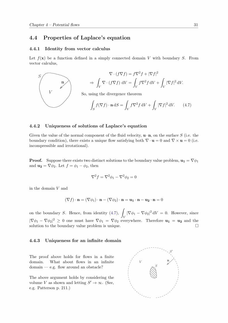
The proof above holds for flows in a finitedomain. What about flows in an infinitedomain — e.g. flow around an obstacle?
The above argument holds by considering thevolume V as shown and letting S′ → ∞. (See,e.g. Patterson p. 211.)
S′
S
Vn
��������
��������

32 4.5 Flow past an obstacle
4.4.4 Kelvin’s minimum energy theorem
Of all possible fluid motions satisfying the boundary condition for u · n on the surface S and∇ · u = 0 in domain V , the potential flow is the flow with the smallest kinetic energy,
K =1
2
∫
Vρ |u|2 dV.
Proof. Let u′ be another incompressible but non vorticity-free flow such that u · n = u′ · non S and ∇ · u′ = 0 in V but with ∇× u′ 6= 0.The fluid flow u is potential, so let u = ∇φ such that
∫
Vρ |u|2 dV =
∫
Vρ|∇φ|2 dV = ρ
∫
V|∇φ|2 dV,
= ρ
∫
Sφu · n dS (by identity (4.7) with f = φ),
= ρ
∫
Sφu′ · n dS (boundary condition),
= ρ
∫
V∇ · (φu′) dV (divergence theorem),
= ρ
∫
Vu′ · ∇φ dV (∇ · u′ = 0),
= ρ
∫
Vu′ · u dV. (4.8)
So,
∫
Vρ (u− u′)2 dV =
∫
V
(
ρ |u|2 − 2ρu · u′ + ρ |u′|2)
dV,
=
∫
V
(
ρ |u′|2 − ρ |u|2)
dV (from (4.8)).
Therefore, since (u− u′)2 ≥ 0,
∫
Vρ |u′|2 dV =
∫
Vρ |u|2 dV +
∫
Vρ (u− u′)2 dV ≥
∫
Vρ |u|2 dV.
�
4.5 Flow past an obstacle
Since the solution to Laplace’s equation for given boundary conditions is unique, if we find a
solution, we have found the solution. (This is only true if the domain is simply-connected; ifthe domain is multiply connected, multiple solutions become possible.)
One technique to calculate non elementary potential flows involves adding together simpleknown solutions to Laplace’s equation to get the solution that satisfies the boundary condi-tions.
4.5.1 Flow around a sphere
We seek an axisymmetric flow of the form u = urer + uzez in cylindrical polar coordi-nates (r, θ, z).

Chapter 4 – Potential flows 33
a
O
U
Z
r
r
n
z
At large distances from the sphere of ra-dius a the flow is asymptotic to a uni-form stream, ur = 0, uz = U , and at thesphere’s surface, r = a, the fluid velocitymust satisfy u ·n = 0 since the solid bodyforms a non-penetrable boundary.
The unit vector normal to surface of the sphere is
n = nrer + nzez with nr =r
aand nz =
z
a.
So, the boundary condition u · n = 0 implies that
urr
a+ uz
z
a= 0 ⇔ rur + zuz = 0
at the spherical surface of equation r2 + z2 = a2.
At large distances, the flow is essentially uniform along the z-axis,
φ ≃ Uz, for ‖r‖ ≫ a.
Now, add to the uniform stream a dipole velocity field of strength µ = µez at the origin,
φ(r, z) = Uz − µz
(r2 + z2)3/2,
so that
ur =∂φ
∂r=
3µrz
(r2 + z2)5/2and uz =
∂φ
∂z= U +
µ
(r2 + z2)3/2
(
3z2
r2 + z2− 1
)
.
Thus, at the sphere’s surface,
u · n = urr
a+ uz
z
a=z
a
(
U +3µ(r2 + z2)
(r2 + z2)5/2− µ
(r2 + z2)3/2
)
,
=z
a
(
U +2µ
(r2 + z2)3/2
)
=z
a
(
U +2µ
a3
)
,
since r2+ z2 = a2. Hence the boundary condition u ·n = 0 at the sphere’s surface determinesthe strength of the dipole,
µ = −Ua3
2.
The velocity potential for a uniform flow past a stationary sphere is therefore given by
φ(r, z) = Uz
(
1 +a3
2(r2 + z2)3/2
)
. (4.9)
The corresponding Stokes streamfunction isgiven by
Ψ(r, z) =Ur2
2
(
1− a3
(r2 + z2)3/2
)
. (4.10)
Outside the sphere Ψ > 0, but we also obtain a solution inside the sphere with Ψ < 0. Thisflow is not real; it is a “virtual flow” that allows for fluid velocity to be consistent with theboundary condition on a solid sphere.

34 4.5 Flow past an obstacle
4.5.2 Rankine half-body
Suppose that, in the velocity potential of a flow past a sphere, we replace the dipole with apoint source (m > 0), so that
φ(r, z) = Uz − m
(r2 + z2)1/2⇒ u = ∇φ =
(
mr
(r2 + z2)3/2, U +
mz
(r2 + z2)3/2
)
.
This flow has a single stagnation point ur = uz = 0 at r = 0 and z = −√
m/U .
To find the streamlines of the flow we calculate the Stokes streamfunction using
ur = −1
r
∂Ψ
∂zand uz =
1
r
∂Ψ
∂r.
Thus,
∂Ψ
∂r= Ur +
mrz
(r2 + z2)3/2⇒ Ψ =
Ur2
2− mz
(r2 + z2)1/2+ α(z),
⇒ 1
r
∂Ψ
∂z= − m
r (r2 + z2)1/2+
mz2
r (r2 + z2)3/2+α′(z)
r,
= −mr
(
r2 + z2 − z2)
(r2 + z2)3/2+α′(z)
r= − mr
(r2 + z2)3/2+α′(z)
r,
= −ur = − mr
(r2 + z2)3/2.
So, since α′(z) = 0, α is a constant (set to zero). The Stokes streamfunction is therefore
Ψ(r, z) =Ur2
2− mz
(r2 + z2)1/2.
At the stagnation point (r = 0, z = −√
m/U), Ψ = m. Hence, the equation of the streamline,or streamtube, passing through this stagnation point is
Ψ(r, z) = m⇔ Ur2
2= m
(
1 +z
(r2 + z2)1/2
)
.
Notice that the straight line r = 0 with z < 0 satisfies the equation of the streamline Ψ = m.For large positive z, the equation of the streamtube Ψ = m becomes
Ur2
2≃ 2m⇒ r ≃ 2
√
m
U.
Thus, the velocity potential and the Stokes streamfunction
φ(r, z) = U
(
z − a2
4 (r2 + z2)1/2
)
and Ψ(r, z) =U
2
(
r2 − a2z
2 (r2 + z2)1/2
)
provide a model for a long slender body of radius a = 2√
m/U .

Chapter 4 – Potential flows 35
4.6 Method of images
In previous examples we introduced flow singularities (e.g. sources and dipoles) outside of thedomain of fluid flow in order to satisfy boundary conditions at a solid surface.
This technique can also be used to calculate the flow produced by a singularity near a bound-ary; it is then called method of images.
Example 4.1 (Point source near a wall)Consider a point-source of fluid placed at the position (d, 0, 0) (Cartesian coordinates) near asolid wall at x = 0.
In free space (no wall), the potential of thesource is
φ∞ = − m√
(x− d)2 + y2 + z2,
⇒ u∞ =∂φ∞∂x
=m(x− d)
[(x− d)2 + y2 + z2]3/2.
y
x
d
O
So that, at x = 0,
u∞ = − md
(d2 + y2 + z2)3/26= 0,
which is inconsistent with the boundary condition u · n = u · ex = u = 0 at the wall.
To rectify this problem, (i.e. for the flow to satisfy the boundary condition at the wall), weadd a source of equal strength m outside the domain, at (−d, 0, 0). By symmetry, this sourcewill produce an equal but opposite velocity field at x = 0, so that the boundary condition forthe combined flow can be satisfied. The velocity potential for both sources becomes
φ = − m√
(x− d)2 + y2 + z2− m√
(x+ d)2 + y2 + z2,
and the velocity field along the x-axis,
u =∂φ
∂x=
m(x− d)
[(x− d)2 + y2 + z2]3/2+
m(x+ d)
[(x+ d)2 + y2 + z2]3/2.
Clearly, at x = 0, now u = 0 as required.The fluid can slip along the wall howeveras, for x = 0,
v =2my
(d2 + y2 + z2)3/2,
w =2mz
(d2 + y2 + z2)3/2.
x−d 0 d
S
4.7 Method of separation of variables
This is a standard method for solving linear partial differential equations with compatibleboundary conditions.
We shall seek separable solutions to Laplace’s equations, of the form φ(x, y) = f(x)g(y) inCartesian coordinates or φ(r, θ) = f(r)g(θ) in polar coordinates.

36 4.7 Method of separation of variables
Plane polar coordinates. We substitute a potential of the form φ(r, θ) = f(r)g(θ) inLaplace’s equation expressed in plane polar coordinates,
∇2φ =1
r
∂
∂r
(
r∂φ
∂r
)
+1
r2∂2φ
∂θ2= 0,
⇒ g
r
d
dr
(
rdf
dr
)
+f
r2d2g
dθ2= 0,
⇒ r
f
d
dr
(
rdf
dr
)
+1
g
d2g
dθ2= 0, (division by f(r)g(θ)/r2)
⇒ r
f
d
dr
(
rdf
dr
)
= −1
g
d2g
dθ2.
Since the terms on the left and right sides of the equation are functions of independentvariables, r and θ respectively, they must take a constant value, k2 say. Thus we havetransformed a partial differential equation for φ into two ordinary differential equations for fand g,
r
f
d
dr
(
rdf
dr
)
= k2 ⇒ rd
dr
(
rdf
dr
)
− k2f = 0,
1
g
d2g
dθ2= −k2 ⇒ d2g
dθ2+ k2g = 0.
Thus, g(θ) = A cos(kθ) +B sin(kθ). For a 2π-periodic function g, such that g(θ) = g(θ+2π),k must be integer. So
g(θ) = A cos(nθ) +B sin(nθ), n ∈ Z,
and f is solution to
r2d2f
dr2+ r
df
dr− n2f = 0.
Substituting nontrivial functions of the form f = arα gives,
[
α(α− 1) + α− n2]
arα = 0 ⇔ α2 = n2.
The two independent solutions have α = ±n; the general separable solution to Laplace’sequation in plane polar coordinates is therefore
φ(r, θ) =(
Arn +Br−n)
cos(nθ) +(
Crn +Dr−n)
sin(nθ), n ∈ Z, (4.11)
where A, B, C and D are constants to be determined by the boundary conditions.
Separable solutions to Laplace’s equation in spherical polar coordinates can be obtained in asimilar manner, but involves Legendre polynomials Pl(cos(θ)).
Example 4.2 (Cylinder in an extensional flow)Consider the velocity potential
φ(r, θ) =(
Ar2 +Br−2)
cos(2θ)
corresponding to a particular solution to Laplace’s equation of the form (4.11), with n = 2.The radial velocity of this flow is
ur =∂φ
∂r= 2r
(
A− B
r4
)
cos(2θ).

Chapter 4 – Potential flows 37
It vanishes at the surface of a solid cylinder of radius a placed at the origin if B = a4A.Therefore the velocity field
ur = 2Ar
(
1− a4
r4
)
cos(2θ) and uθ = −2Ar
(
1 +a4
r4
)
sin(2θ)
produced by the potential
φ(r, θ) = Ar2(
1 +a4
r4
)
cos(2θ)
represents a fluid flow past a solid cylinder placed in an extensional flow.
Notice that at large distances, i.e. if r ≫ a, thefluid velocity is that of an extensional flow
ur ≃ 2Ar cos(2θ) and uθ ≃ −2Ar sin(2θ),
in polar coordinates, or equivalently
u ≃ 2Ax and v ≃ −2Ay,
in Cartesian coordinates.

38 4.7 Method of separation of variables