Potential performance theory (PPT) was developed by Trafimow and Rice (2008) as a general theory of task per-formance that specifies the relationships among actual per-formance, true performance, and randomness. Although Trafimow and Rice performed mathematical simulations of the theory’s consequences given various starting points, and even performed an illustrative experiment, they did not fully explore the potential of PPT as a methodological tool. We believe that there are such implications and that they are important. Consequently, our main goals are to work out these implications in detail, perform an experiment to demonstrate them, and illustrate how the conclusions drawn from traditional methods are misleading in the ab-sence of the proposed methods. Furthermore, we introduce new mathematical equations that further enhance the use of PPT. To aid in demonstrating this new methodology, we use an example paradigm, whereby participants perform a high-fidelity target- detection task; however, we want to be clear that our goal is to demonstrate the proposed PPT methodology, rather than to contribute extensively to the literature on this particular paradigm.

A SUMMARY OF PPT

PPT is based on the idea that a person’s observed per-formance on a task is influenced by two variables: (1) the combination of the nonrandom factors that are relevant to the performance of the task, which PPT terms strategy, and (2) random factors. For those people whose strategy is better than randomness, it is easy to demonstrate that lack of consistency (randomness) decreases task performance (see Trafimow & Rice, 2008, Figure 1). PPT quantifies what the person’s expected task performance would be if random factors were completely eliminated—that is, if

the person were to execute a perfectly consistent pattern of behavior. In addition, PPT quantifies what the person’s task performance would be under any level of consistency that the researcher desires to consider.

PPT is based, in part, on classical true-score theory. According to classical true-score theory, observed perfor-mance is determined by two factors: a person’s “true” score and random error (for reviews, see Allen & Yen, 1979; Cohen & Swerdlik, 1999; Crocker & Algina, 1986; Lord & Novick, 1968). Interestingly, although random error is, by definition, random, it can have systematic effects on correlation coefficients. As random error increases, cor-relations between variables decrease. Classical true-score theorists derived a “correction” formula that provides the expected value for the true correlation if the measures of the variables are perfectly reliable and have no random error. Specifically, the expected value for the true cor-relation coefficient is based on the observed correlation coefficient, adjusted for the reliability of the measures of the relevant variables. Equation 1 gives the correction for-mula, where R is the true correlation between variables X and Y, and rXX and rYY are the reliabilities of the measures of the two variables, respectively.

R r

r rXX YY

(1)

Because task performance is not usually studied via cor-relation coefficients, it may seem that Equation 1 is not particularly helpful. But here is where PPT comes in: PPT explains how it is possible to take advantage of Equation 1, despite the fact that researchers interested in skill acqui-sition tend not to use correlations. Put briefly, PPT com-mences by assuming a dichotomous task and two blocks of task performance trials. For example, the option for each

359 © 2009 The Psychonomic Society, Inc.

Potential performance theory (PPT): Describing a methodology for analyzing task performance

DAVID TRAFIMOW AND STEPHEN RICENew Mexico State University, Las Cruces, New Mexico

Based on potential performance theory (PPT), a methodological paradigm is developed that allows for individual- level analyses. The proposed methodology distinguishes among observed performance, strategy, and consistency, with the idea that changes in observed performance can be caused by changes in strategy or consistency. Equations are presented that allow the computation of strategy and consistency scores for groups and individuals, with the goal of enabling researchers to find the reasons why performance improves or does not improve. More specifically, people may (1) develop better strategies, (2) use them more consistently, (3) both, or (4) neither. It is even possible to have strategy–consistency trade-offs, as individuals focus on one at the expense of the other. Data obtained from an experiment illustrate these possibilities.

Behavior Research Methods2009, 41 (2), 359-371doi:10.3758/BRM.41.2.359

D. Trafimow, dtrafimo@nmsu.edu; S. Rice, sc_rice@yahoo.com

360 TRAFIMOW AND RICE

mance table is based on an adjusted correlation coefficient that takes inconsistency into account, it will henceforth be termed a true table. To indicate that the frequencies in the new table are estimates of true scores, they will be denoted by uppercase letters. Thus, A, B, C, and D indicate estimates of true-score cell frequencies, and R1, R2, C1, and C2 indi-cate the fixed margin frequencies.1 Equations 4, 5, 6, and 7 give the true frequency estimates for cells A, B, C, and D, respectively. Alternatively, once Equation 4 is used to find A, the other cells can be determined by subtraction from the appropriate row or margin frequencies.

AR R R C C C R

R R1 2 1 2 1 1

1 2

.

(4)

BR R R R R R C C C R

R R1 1 2 1 2 1 2 1 1

1 2

.

(5)

CC R R R R C C

R R1 2 1 2 1 2

1 2

.

(6)

D

C R R R R R R R R C C C R

R

2 1 2 1 1 2 1 2 1 2 1 1

11 2R.

(7)

METHODOLOGICAL IMPLICATIONS FOR PRACTICE STUDIES

If a person’s observed performance is close to perfect, it is easy to deduce that she must have had a good strategy and used it consistently. Less clear, but of more interest, is when a person’s observed performance is in the interme-diate range; that is, the person’s observed performance is better than randomness, but also far from perfect. In this case, there are many possibilities. At one extreme, the per-son might have an optimal strategy, but uses it inconsis-tently. At the other extreme, the person might have a poor strategy, but uses it consistently. To the extent that strate-gies approach optimality, poor performance is caused by lack of consistency. And to the extent that strategies are poor (but better than randomness), intermediate observed performance might nevertheless be achieved by their con-sistent use. Thus, inconsistent use of a good strategy will result in a decrease in observed performance, and consis-tent use of even a bad strategy might nevertheless result in reasonably good observed performance.

Let us now consider these issues in the context of practice studies. Suppose that a researcher conducts a practice study, finds that the experimental condition mean exceeds the con-trol condition mean, and concludes that practice improved performance. Of course, researchers recognize the fallacy of concluding that the practice caused everyone to improve; rather, the conclusion researchers would draw is that, on av-erage, there was improvement. But this vague type of caveat is not satisfactory. Why did some people not improve? It could be because they were not influenced by the practice. Alternatively, the practice might have endowed them with

trial might be “yes” or “no,” and the correct answer might be “yes” or “no.” Across all of the trials, then, it is pos-sible to construct a 2 (option chosen) 2 (correct option) frequency table giving the number of times the person an-swered “yes” correctly or incorrectly (in signal detection theory terms, these are hits and false alarms, respectively) and the number of times the person answered “no” cor-rectly or incorrectly (in signal detection theory terms, these are correct rejections and misses, respectively).

Although PPT and signal detection theory use similar 2 2 tables, they deal with different issues. The former distinguishes between strategy and consistency, whereas the latter distinguishes between sensitivity and bias. Therefore, the two theories are not interchangeable, nor can one be substituted for the other.

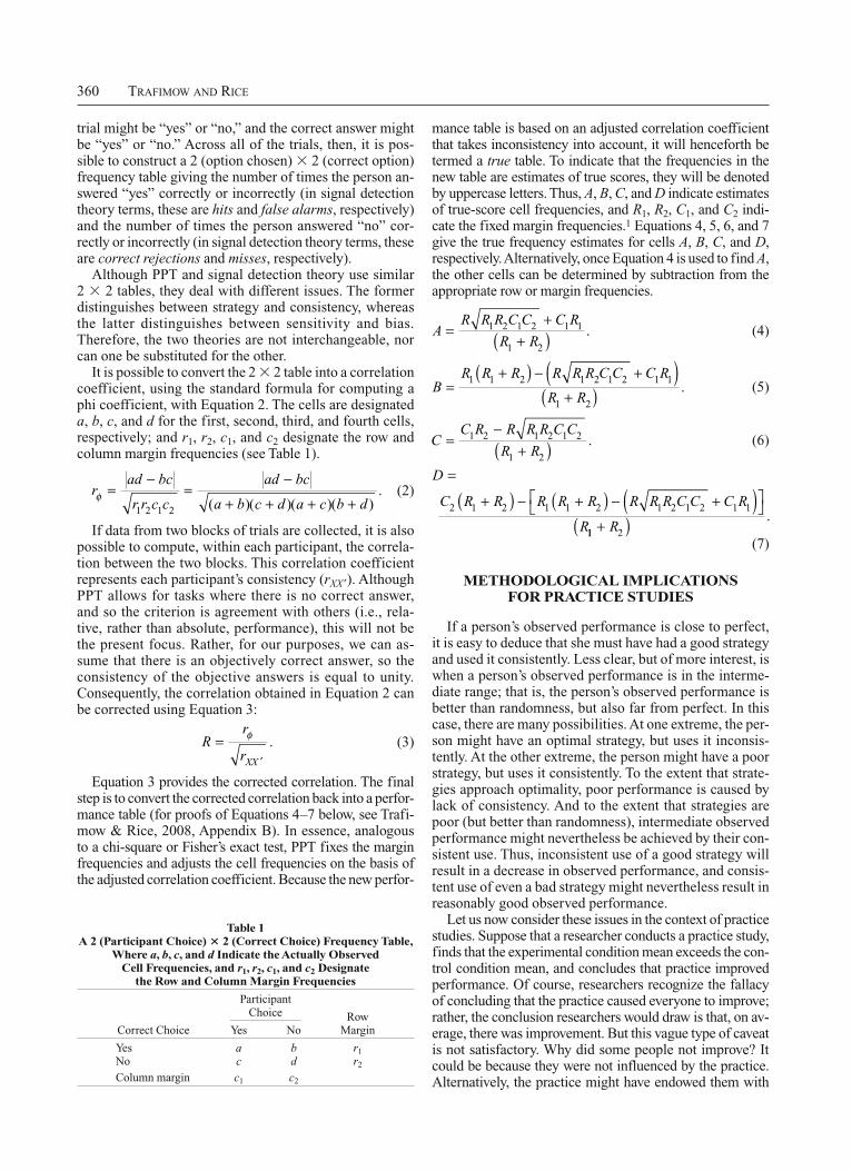
It is possible to convert the 2 2 table into a correlation coefficient, using the standard formula for computing a phi coefficient, with Equation 2. The cells are designated a, b, c, and d for the first, second, third, and fourth cells, respectively; and r1, r2, c1, and c2 designate the row and column margin frequencies (see Table 1).

r

ad bc

r r c c

ad bc

a b c d a c b d1 2 1 2 ( )( )( )( ).

(2)

If data from two blocks of trials are collected, it is also possible to compute, within each participant, the correla-tion between the two blocks. This correlation coefficient represents each participant’s consistency (rXX ). Although PPT allows for tasks where there is no correct answer, and so the criterion is agreement with others (i.e., rela-tive, rather than absolute, performance), this will not be the present focus. Rather, for our purposes, we can as-sume that there is an objectively correct answer, so the consistency of the objective answers is equal to unity. Consequently, the correlation obtained in Equation 2 can be corrected using Equation 3:

R

r

rXX

.

(3)

Equation 3 provides the corrected correlation. The final step is to convert the corrected correlation back into a perfor-mance table (for proofs of Equations 4–7 below, see Trafi-mow & Rice, 2008, Appendix B). In essence, analogous to a chi-square or Fisher’s exact test, PPT fixes the margin frequencies and adjusts the cell frequencies on the basis of the adjusted correlation coefficient. Because the new perfor-

Table 1 A 2 (Participant Choice) 2 (Correct Choice) Frequency Table,

Where a, b, c, and d Indicate the Actually Observed Cell Frequencies, and r1, r2, c1, and c2 Designate

the Row and Column Margin Frequencies

ParticipantChoice Row

Correct Choice Yes No Margin

Yes a b r1No c d r2

Column margin c1 c2

PPT METHODOLOGY 361

of interest.) In all equations, the subscript DES indicates that these are estimates of desired values, rather than ac-tually observed or true values. Thus, the desired adjusted correlation giving the desired goodness of the strategy is RDES; the desired level of consistency is rDES–XX ; and the desired cell frequencies are ADES, BDES, CDES, and DDES.

A Methodological Paradigm Derived From PPTTo use PPT, it is necessary to have two blocks of task

performance trials, so that consistency and observed per-formance can be measured. Subsequent to practice, it is necessary to have two more blocks of task performance trials, for a total of at least two sessions of two blocks of task performance trials. This may seem repetitious, but it is necessary to allow for observed performance and con-sistency to be assessed before and after practice. Given that observed performance and consistency are obtained for each participant both before and after practice, PPT allows for the calculation of true performance both be-fore and after practice. In summary, whether because of direct observation or because of using PPT equations, the researcher will have values for observed performance, consistency, and true performance, both before and after practice, for every participant in the experiment.

At this point, answers to the questions brought up in the foregoing section can be derived mathematically. Let us consider, for example, a hypothetical Participant A, whose observed performance did not improve from prepractice to postpractice. If consistency was unchanged as well, it is clear that the training failed to influence Participant A. But suppose that Participant A’s consistency actually decreased from prepractice to postpractice, but his observed perfor-mance remained unchanged. In that case, it is clear that the practice must have provided him with a better strategy that balanced out the decrease in consistency. In this case, it would be a mistake to conclude that the practice did not do anything. Rather, the practice had a positive effect on strategy and a negative effect on consistency, and the two balanced each other out. Perhaps simple rehearsal of the new strategy would increase consistency too, thereby resulting in increased observed performance.

Let us consider hypothetical Participant B, whose observed performance did increase from prepractice to postpractice. Did the practice provide her with a better strategy? There are multiple possibilities. If consistency

a better strategy, but they might have used it with less con-sistency. Superior strategy and inferior consistency might balance each other out to result in zero improvement in ob-served performance. And for those who did improve, why did they improve? The practice could have improved their strategy, or their consistency, or both. It would be desirable to know how much strategy and consistency improved, and how much each of these improvements contributed to the improvement in people’s observed performance. It is even possible that there is a joint effect, whereby improvements in both strategy and consistency combine in a nonadditive way. We hope to demonstrate a methodology that can answer these important, but previously intractable, questions.2

Deriving Desired Cell ValuesWhen setting up the proposed methodology, it is impor-

tant to distinguish among three types of cell values. We have already discussed observed cell values (a, b, c, d ) and estimates of true cell values (A, B, C, D). There are also desired cell values: the best estimates of values that would be obtained given any desired level of observed cell values and consistency that the researcher wishes to investigate. Because the focus of the original PPT article is theoretical, it does not provide the required mathematics to serve our present methodological purposes, so it will be necessary to provide new derivations here. To see the necessity for deriving desired cell values, consider, for example, that one might wish to know how much of a dif-ference an increase in consistency would make, keeping strategy (i.e., true successes) constant. Or one might wish to know how much of a difference an increase in strategy would make, keeping consistency constant. Finally, one might wish to know how much the joint effect of a change in consistency and a change in strategy would influence observed successes above and beyond that which would be obtained from either change alone.

Equations 8–11 (see below) provide the means for ob-taining the desired cell values, given that the values for the adjusted correlation indicating the goodness of the strategy (RDES) and consistency (rDES–XX ) are set at whatever levels the experimenter wishes to explore. These equations are derived in Appendix A. (Although unnecessary for analyz-ing the data to be presented, Appendix B provides a deriva-tion of equations that can be used for analyzing data where relative performance, rather than absolute performance, is

A

R r R R C C C R

R RXX

DESDES DES 1 2 1 2 1 1

2 1 (8)

B

R R R R r R R C C C R

RXX

DESDES DES1 1 2 1 2 1 2 1 1

22 1R (9)

C

C R R r R R C C

R RXX

DESDES DES1 2 1 2 1 2

2 1 (10)

D

C R R R R R R r R R CXX

DES

DES DES2 1 2 1 1 2 1 2 1CC C R

R R

2 1 1

2 1 (11)

362 TRAFIMOW AND RICE

effect of the change of consistency on observed successes, controlling for strategy.

Controlling for consistency. The researcher may wish to assess the effect of a change in strategy on observed successes, if consistency for the postpractice trials re-mained at the prepractice level. In other words, it is some-times useful to calculate the effect of a change in strategy, controlling for consistency. To do this, the foregoing steps can be followed, with the exception that modifications of Step 1 and Step 2 are necessary.

Modified Step 1. To obtain true values for R, A, B, C, and D, use Equations 3–7, respectively, on the prepractice data, as before. In addition, obtain R from the postprac-tice data by first obtaining r from the actually obtained postpractice data according to Equation 2 and adjusting it using Equation 3.

Modified Step 2. Instantiate the desired values into Equations 8–11.

a. Set RDES at the value that was obtained for R during the postpractice block.b. Set rDES XX at the level that was obtained for rXX during the prepractice block.Obtaining the joint effect. To obtain the predicted

joint effect in the postpractice session, it is merely neces-sary to use the foregoing procedure, but with yet another slight modification of Step 2.

Further Modified Step 2. Instantiate the desired values into Equations 8–11.

a. Set RDES at the value that was obtained for R dur- ing the postpractice block.b. Set rDES XX at the level that was obtained for rXX during the postpractice block.The foregoing procedures give (1) the effect of change of

consistency on observed successes, controlling for change in strategy; (2) the effect of change of strategy on observed successes, controlling for change in consistency; and (3) the predicted joint effect of changes in strategy and consistency based on the strategy and consistency in the postpractice session, but using the margin frequencies from the pre-practice session. To the extent that the predicted joint effect exceeds the effect of consistency (controlling for strategy) and the effect of strategy (controlling for consistency), the researcher has an indication of how much power the joint effect has above and beyond the individual effects of change in consistency and change in strategy.

Remember that an important assumption made by PPT is that the margin frequencies can be fixed, which justifies the use of prepractice margin frequencies. To the extent that this assumption is wrong, the actual joint effect, exem-plified by the actually observed proportion of postpractice successes, should differ from the predicted joint effect, calculated using prepractice margin frequencies. This as-sumption can be tested by correlating predicted and actu-ally observed joint effects, as will be demonstrated later.

The following experiment was performed to test all of these possibilities within the context of a high-fidelity target-detection experiment. As is common with experi-ments that measure performance effects over time, (1) the task was repetitive; (2) the task was difficult enough to reveal performance improvements; (3) feedback was pro-

did not increase, it is clear that the better observed per-formance can be attributed solely to an improvement in strategy, which should be reflected by a true performance increase. If true performance did not increase, it is clear that the practice must have improved consistency, which should be reflected by an improved consistency score from prepractice to postpractice. Now, suppose that there was a large improvement in observed performance, coupled with small improvements in consistency and true performance. And suppose that even the additive effects of the improve-ments in consistency and true performance cannot fully account for the improvement in observed performance. In this case, it is clear that some of the improvement in ob-served performance must have been due to the joint effect of improved consistency and strategy.

It is possible to restate the foregoing points more pre-cisely, considering that Equations 8–11 can be used in at least three ways. The first way is to find out what the success rate would be at any particular level of consis-tency that the experimenter wishes to test. For example, suppose that a person’s true score and consistency both change from prepractice to postpractice. It is an easy mat-ter to obtain observed and true tables from both sessions, given Equations 4–7. It is also an easy matter to obtain the consistency coefficient (rXX ) from the data, and the adjusted correlation coefficient (R) from Equation 3. But how would the change in consistency have influenced the observed proportion of successes if there had been no change in strategy? To answer this question, the researcher would perform the following steps.

Controlling for strategy. The following steps allow the researcher to determine the effect of the change in con-sistency while controlling for any change in strategy that might have occurred.

Step 1. To obtain true values for R, A, B, C, and D, use Equations 3–7, respectively, on the prepractice data. Remem-ber to fix the margin frequencies at the obtained values.

Step 2. Instantiate the desired values into Equa-tions 8–11.

a. Set RDES at the value that was obtained for R dur- ing the prepractice block.b. Set rDES XX at the level that was obtained for rXX during the postpractice block.Step 3. Solve Equations 8–11 based on the instantiated

values.Step 4. The desired level of total successes (TDES) is

obtained by the cells along the major diagonal. In math-ematical notation, TDES ADES DDES.

Step 5. The desired proportion of successes (PDES) is obtained by dividing the result from Step 4 by the number of trials. In mathematical notation,

P

T

R RDESDES

1 2

.

Step 6. Subtracting from PDES the observed proportion of successes obtained from the prepractice trials gives the difference that the change in consistency made in ob-served successes, keeping the goodness of the strategy at the same level in the postpractice trials as it was in the prepractice trials. Put another way, the difference is the

PPT METHODOLOGY 363

was available to answer any questions. The instructions included a picture of the simulated tank. Participants pressed a key on the key-board when they were ready to begin the experiment.

Participants were presented with five sessions of 100 trials each. Each session lasted approximately 20–30 min and consisted of two blocks of 50 trials per block. Within each session, participants viewed identical trials across the two blocks. This was done to pro-vide consistency measures, as required by PPT. Participants were given a 5-min break between each block and session.

Each trial began with a blank screen followed by the image display on a white background. The aerial image was presented for 4 sec, which, based on prior research using this same task, is the average amount of time people tend to take to inspect a single aerial image (Rice et al., in press). Subsequently, a choice display was presented with the following question: “Was there a tank present? J Yes, F No.” Participants then had 10 sec to press the appropriate key to re-cord their response. Following this, a feedback display appeared for 1 sec, informing the participants whether they were correct or not.

ResultsA downloadable macro of the program we created to

conduct PPT analyses can be found at www.stephenrice .us/macro.html. Five types of results are presented. In the first section, the data were analyzed traditionally, and the resulting traditional conclusion is presented. Second, means of PPT analyses across the sample are presented. Third, PPT analyses on individuals, based on why their performances improved (or, in a few cases, did not im-prove), are presented. Fourth, the evolution of the skill ac-quisition process is considered. Finally, the ability of PPT to predict observed postpractice performance is assessed.

Traditional analyses. To perform a traditional test of the effects of practice on performance, we performed a 5 (session) 2 (block) within-participants ANOVA. We obtained a main effect of session (M1 .73, M2 .79, M3 .81, M4 .84, M5 .86) [F(1,23) 18.90, p .05,

2p .451]. A polynomial analysis on these means shows

a significant linear trend, but the higher order trends were not significant. In addition, there was no significant effect of blocks, nor was the session effect qualified by a ses-sion block interaction.

Group PPT analyses. The foregoing analyses indicate that, on average, practice improved observed performance. However, it is desirable to assess whether there also were parallel effects on PPT variables. In fact, strategy (indexed by true performance) improved across sessions (M1 .80, M2 .84, M3 .87, M4 .91, M5 .91), the difference from M1 to M5 being .11. Consistency also improved (M1 .46, M2 .69, M3 .69, M4 .71, M5 .80), the difference from M1 to M5 being .34. Clearly, at least at the group level, the data indicate that both PPT variables were influenced by practice, thereby improving observed performance.

Individual-level PPT analyses. With 24 participants to consider, it is difficult to present individual-level analy-ses in a coherent manner. We arbitrarily defined improve-ment as an increase of at least .05 from the first session to the fifth session for strategy, and as an increase of at least .10 from the first session to the fifth session for con-sistency. Thus, this section is organized in terms of par-ticipants who improved in strategy but not in consistency, participants who improved in consistency but not in strat-egy, and participants who improved in both categories.

vided on all trials; (4) the participants were motivated to do well and improve their performance; and (5) the entire session took less than 2 h.

THE PRESENT EXPERIMENT

To test the effectiveness of the proposed methodologi-cal paradigm, we chose to use a task in which people were presented with aerial photographs and were asked to detect whether or not there was an enemy target present (Rice, in press; Rice, Trafimow, Clayton, & Hunt, in press). Al-though this task may seem more complex than absolutely necessary, there were two reasons for using it. First, our previous research indicated that the task was sufficiently difficult to allow room for practice to cause improvement (Rice, in press; Rice et al., in press). Second, because of our previously having conducted similar research, the pro-gramming had already been done, making the present task convenient to use.

To make it possible to calculate each participant’s con-sistency within each of the four sessions, there were two blocks of trials within each session. Of course, we were also able to calculate observed performance in terms of the per-centage of times the person detected the target when it was there (hit), did not detect the target when it was there (miss), detected the target when it was not there (false alarm), and did not detect the target when it was not there (correct re-jection). From the combination of consistency data and ob-served performance, Equations 1–7 were used to estimate true cell frequencies for the 2 2 table, from which it was possible to compute the adjusted correlation coefficient and true performance (our index of strategy), for each partici-pant for each session of two blocks of 50 trials.

MethodParticipants. Twenty-four members of the New Mexico State

University community (12 female) participated in the experiment for course credit. To ensure that the task would be novel, and thus provide room for the training to be effective, none of the participants were selected for their expertise in analyzing aerial photographs. The mean age was 20.8 years (SD 3.9). Participants were screened for normal or corrected-to-normal visual acuity, using a Snellen eye chart, and for color vision, using Ishihara’s Tests for Color-Blindness.

Material and Stimuli. The experiment was presented on a Dell PC with a 2.0-GHz processor, using a 20-in. monitor with 1,024 768 resolution and a 65-Hz refresh rate. Participants were seated ap-proximately 21 in. from the monitor, with head position controlled by a chinrest.

Target-present trials were created by digitally blending a simulated tank onto 25 aerial images of Baghdad taken from approximately 6,000 ft in altitude, which is typical for this type of aerial inspec-tion when conducting military surveillance. This was done using Photoshop CS2; the tank was placed randomly within the confines of the photograph, and then the two layers were digitally merged. Target-absent trials were created by using the same 25 aerial images without the tank. The tank took up approximately 2º 2º of visual angle, which guaranteed that it would not be disproportional to the rest of the landscape features (e.g., buildings), and was displayed in one of eight randomly assigned orientations facing north, northeast, east, southeast, south, southwest, west, or northwest. The order of presentation was randomized for each participant.

Procedure and Design. Participants first signed a consent form and were then seated in a comfortable chair facing the experimental display. Instructions were presented on-screen, and an experimenter

364 TRAFIMOW AND RICE

Note that the multiplicative effect of the two increases greatly outstrips the improvement that would have been engendered by either increase alone, or even by the addi-tion of the two increases.

Observed performance did not improve by at least .05. Four participants failed to improve by at least .05. According to PPT, there are two ways for a person not to change much in observed performance. First, there might be very little change in strategy and consistency. For example, Participant 21 improved by only .02 in strategy and .08 in consistency, netting an improvement of only .04 in observed perfor-mance. Second, and more interestingly, however, a person could change markedly in both strategy and consistency, but in opposite directions, thereby rendering very little change in observed performance. Participant 8 provides a nice ex-ample of this. This participant increased by .39 in consis-tency, but decreased by .08 in strategy, for a net increase in observed performance of only .02. Note that, had strategy remained unchanged, this participant would have improved by an impressive .09, and, had consistency remained un-changed, the observed score would have decreased by .03.

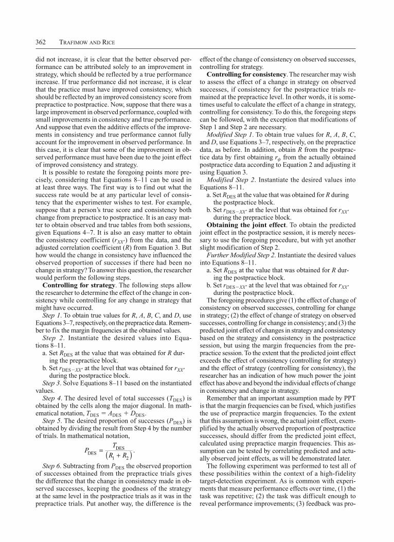
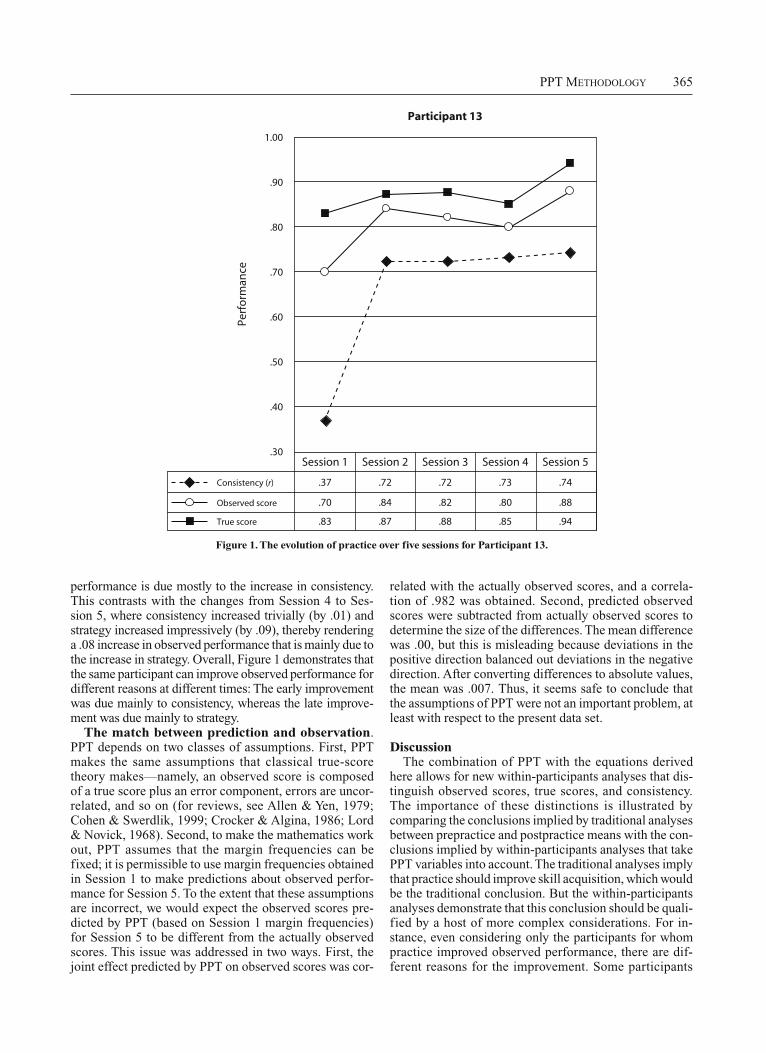
The evolution of practice. Researchers may be inter-ested in changes in observed performance, strategy, and consistency across all of the sessions. In our opinion, the easiest way to get an idea of how these changes evolve over sessions is to graph the variables, but separately for each participant. Figure 1 illustrates the possibilities that arise from this type of analysis. In Figure 1, the true performance, consistency, and observed performance of Participant 13 is shown across all five sessions. From Session 1 to Session 2, this participant increased only .04 in strategy, but increased by .34 in consistency. Thus, the .14 increase in observed

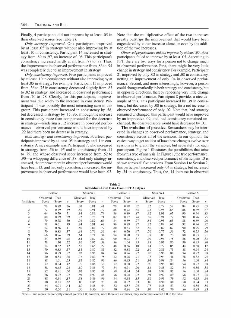
Finally, 4 participants did not improve by at least .05 in their observed scores (see Table 2).

Only strategy improved. One participant improved by at least .05 in strategy without also improving by at least .10 in consistency. Participant 14 increased in strat-egy from .89 to .97, an increase of .08. This participant’s consistency increased hardly at all, from .87 to .88. Thus, the improvement in observed performance from .86 to .94 was completely due to an improvement in strategy.

Only consistency improved. Five participants improved by at least .10 in consistency without also improving by at least .05 in strategy. For example, Participant 15 improved from .36 to .75 in consistency, decreased slightly from .83 to .82 in strategy, and increased in observed performance from .70 to .78. Clearly, for this participant, improve-ment was due solely to the increase in consistency. Par-ticipant 11 was possibly the most interesting case in this group: This participant increased in consistency by .58, but decreased in strategy by .15. So, although the increase in consistency more than compensated for the decrease in strategy—rendering a .12 increase in observed perfor-mance—observed performance would have improved by .22 had there been no decrease in strategy.

Both strategy and consistency improved. Fourteen par-ticipants improved by at least .05 in strategy and .1 in con-sistency. A nice example was Participant 7, who increased in strategy from .56 to .95 and in consistency from .11 to .79, and whose observed score increased from .52 to .90—a whopping difference of .38. Had only strategy in-creased, the improvement in observed performance would have been .13; and had only consistency increased, the im-provement in observed performance would have been .03.

Table 2 Individual-Level Data From PPT Analyses

Session 1 Session 2 Session 3 Session 4 Session 5

Observed True Observed True Observed True Observed True Observed TrueParticipant Score Score r Score Score r Score Score r Score Score r Score Score r

1 .70 0.89 .26 .70 0.81 .41 .70 0.78 .52 .72 0.79 .57 .84 0.93 .632 .72 0.79 .59 .86 0.91 .79 .88 0.92 .84 .92 0.95 .88 .86 0.89 .873 .64 0.70 .51 .84 0.89 .74 .86 0.89 .87 .92 1.01 .67 .90 0.94 .834 .80 0.89 .59 .72 0.76 .71 .82 0.87 .74 .86 0.91 .79 .90 0.96 .755 .70 0.78 .50 .76 0.82 .66 .84 0.89 .77 .84 0.93 .63 .88 0.89 .966 .58 0.61 .49 .84 0.91 .68 .86 0.89 .87 .82 0.89 .67 .92 0.94 .927 .52 0.56 .11 .80 0.84 .77 .80 0.83 .82 .86 0.89 .87 .90 0.95 .798 .70 0.83 .37 .68 0.79 .39 .64 0.70 .47 .70 0.77 .56 .72 0.75 .769 .66 0.76 .39 .64 0.74 .34 .74 0.80 .63 .78 0.83 .70 .80 0.83 .81

10 .84 0.89 .75 .84 0.87 .87 .90 0.93 .87 .90 0.96 .75 .86 0.90 .8311 .78 1.10 .22 .86 0.97 .58 .86 1.04 .45 .88 0.93 .80 .90 0.95 .8012 .54 0.62 .12 .58 0.65 .27 .48 0.56 .10 .44 0.77 .05 .44 0.68 .1213 .70 0.83 .37 .84 0.87 .83 .82 0.88 .72 .80 0.85 .73 .88 0.94 .7414 .86 0.89 .87 .92 0.96 .84 .94 0.96 .92 .90 0.93 .88 .94 0.97 .8815 .70 0.83 .36 .76 0.80 .75 .72 0.76 .71 .78 0.94 .41 .78 0.82 .7516 .88 1.01 .55 .84 0.85 .96 .86 0.93 .71 .94 0.98 .84 .96 1.00 .8417 .72 0.84 .42 .78 0.86 .59 .82 0.88 .72 .90 0.95 .80 .94 0.97 .8818 .58 0.65 .28 .80 0.85 .73 .84 0.91 .70 .84 0.88 .82 .84 0.86 .8819 .82 0.91 .60 .92 0.97 .81 .88 0.94 .74 .94 0.99 .82 .96 1.00 .8420 .86 0.92 .72 .94 0.97 .88 .96 0.98 .92 .94 0.97 .89 .96 0.97 .9621 .88 0.91 .87 .88 0.89 .96 .94 0.98 .85 .86 0.91 .79 .92 0.93 .9622 .78 0.85 .62 .80 0.85 .73 .88 0.92 .83 .88 0.90 .88 .90 0.94 .8323 .64 0.71 .44 .80 0.88 .64 .82 0.87 .76 .78 0.88 .53 .82 0.86 .8024 .50 0.50 .11 .50 0.50 .14 .40 0.86 .08 .94 1.02 .70 .86 0.89 .83

Note—True scores theoretically cannot go over 1.0; however, since these are estimates, they sometimes exceed 1.0 in the table.

PPT METHODOLOGY 365

related with the actually observed scores, and a correla-tion of .982 was obtained. Second, predicted observed scores were subtracted from actually observed scores to determine the size of the differences. The mean difference was .00, but this is misleading because deviations in the positive direction balanced out deviations in the negative direction. After converting differences to absolute values, the mean was .007. Thus, it seems safe to conclude that the assumptions of PPT were not an important problem, at least with respect to the present data set.

DiscussionThe combination of PPT with the equations derived

here allows for new within-participants analyses that dis-tinguish observed scores, true scores, and consistency. The importance of these distinctions is illustrated by comparing the conclusions implied by traditional analyses between prepractice and postpractice means with the con-clusions implied by within-participants analyses that take PPT variables into account. The traditional analyses imply that practice should improve skill acquisition, which would be the traditional conclusion. But the within- participants analyses demonstrate that this conclusion should be quali-fied by a host of more complex considerations. For in-stance, even considering only the participants for whom practice improved observed performance, there are dif-ferent reasons for the improvement. Some participants

performance is due mostly to the increase in consistency. This contrasts with the changes from Session 4 to Ses-sion 5, where consistency increased trivially (by .01) and strategy increased impressively (by .09), thereby rendering a .08 increase in observed performance that is mainly due to the increase in strategy. Overall, Figure 1 demonstrates that the same participant can improve observed performance for different reasons at different times: The early improvement was due mainly to consistency, whereas the late improve-ment was due mainly to strategy.

The match between prediction and observation. PPT depends on two classes of assumptions. First, PPT makes the same assumptions that classical true-score theory makes—namely, an observed score is composed of a true score plus an error component, errors are uncor-related, and so on (for reviews, see Allen & Yen, 1979; Cohen & Swerdlik, 1999; Crocker & Algina, 1986; Lord & Novick, 1968). Second, to make the mathematics work out, PPT assumes that the margin frequencies can be fixed; it is permissible to use margin frequencies obtained in Session 1 to make predictions about observed perfor-mance for Session 5. To the extent that these assumptions are incorrect, we would expect the observed scores pre-dicted by PPT (based on Session 1 margin frequencies) for Session 5 to be different from the actually observed scores. This issue was addressed in two ways. First, the joint effect predicted by PPT on observed scores was cor-

1.00

.90

.80

.70

.60

.50

.40

.30

Perf

orm

ance

Participant 13

Consistency (r)

Observed score

True score

.37

.70

.83

Session 1

.72

.84

.87

Session 2

.72

.82

.88

Session 3

.73

.80

.85

Session 4

.74

.88

.94

Session 5

Figure 1. The evolution of practice over five sessions for Participant 13.

366 TRAFIMOW AND RICE

nition and human factors literature is full of examples where PPT could provide additional and potentially counter intuitive information regarding the tasks at hand. For example, recent studies have analyzed the difference between 2-D and 3-D displays in aviation (e.g., Alexander, Wickens, & Hardy, 2005; Thomas & Wickens, 2006), with mixed conclusions (that each display is more beneficial for a particular type of task). However, a reanalysis using PPT could lead to a better understanding of why each par-ticular display is more useful for a particular task; that is, do different displays invoke different strategies, depend-ing on the task, or do they influence the consistency of behavior, again depending on the task?

PPT also can be extended beyond psychology into other areas of research, including economics, philosophy, educa-tion, and others. In economics, much is made of the teaching techniques used to improve stock-picking abilities. How-ever, do these techniques actually improve stock- picking strategies, the consistencies with which brokers choose stocks, or both? Of course, interest in teaching techniques is not limited to economics, but can apply to all areas of education as well. When we teach children new methods in mathematics or in the sciences, are they improving via these new strategies, or are they learning to be more consistent? Via PPT methodology, teachers and parents can learn a lot about how to improve children’s performance.

In medicine, there is concern about training radiologists to improve their scanning techniques while inspecting pa-tients’ X-rays. Expert radiologists tend to have more effi-cient scan patterns with shorter fixation durations than do novices (e.g., Kundel & LaFollette, 1972; Lesgold et al., 1988; Revesz & Kundel, 1977). However, it is not clear whether these improvements are due to new strategies or to a more consistent pattern of inspection. Kundel and La-Follette found an evolution of visual scanning behavior with increased experience in radiology and pointed out that the visual scanning patterns experts had developed did not correspond to any instructional patterns taught in class or presented in textbooks. Gale and Worthington (1983) adopted a search strategy that was based on a sur-vey given to expert radiologists and coached participants to use it in a radiology task. Their results indicated that a training group did indeed employ the training strategy, but that it was not beneficial to their overall performance. The authors concluded that training radiologists to adopt a spe-cific search pattern was not worthwhile. These studies lack the ability to analyze individual strategies and consisten-cies on a case-by-case basis. Perhaps consistency plays a much bigger role in radiology—and in other visual-search or quality-control tasks (e.g., Schoonard, Gould, & Miller, 1973)—than has previously been apparent.

PPT methodology is not limited to humans. Automation studies in the past 20 years have attempted to explain the interaction between humans and automation during per-formance tasks (e.g., Bainbridge, 1983; Dixon & Wick-ens, 2006; Dixon, Wickens, & Chang, 2005; Dixon, Wick-ens, & McCarley, 2007; Lee & Moray, 1994; Parasuraman & Riley, 1997; Parasuraman, Sheridan, & Wickens, 2000; Rice, in press; Rice et al., in press; Wickens & Dixon, 2007). Unfortunately, most of these studies do not analyze

gained by improving their strategy, some by improving their consistency, and some by improving both. Some of these participants actually decreased in either strategy or consistency, but more than countered that decrease with an increase in the other variable, thereby resulting in a net increase in observed performance.

Four of the 24 participants failed to demonstrate im-provement in observed scores after practice. For some, this was because practice did not have much of an influence on either strategy or consistency, thereby leaving observed performance relatively unchanged. But for others, there was a substantial change in either strategy or consistency that was countered by a change in the other variable in the opposite direction, thereby resulting in little or no net effect on observed performance. Failing to assess strategy and consistency might cause one to erroneously conclude that practice did not change anything for these individu-als; whereas the truth of the matter may be that it caused changes in two variables, albeit in opposite directions.

In addition, the proposed methodology renders possible conclusions not only about why practice has the effects that it has (or does not have) on observed performance, but also about how these effects evolve over sessions. Figure 1 further demonstrates that, even within the same individual, the causes of improved observed performance can differ at different points in the learning process.

Other tasks. A main concern of the present article was to derive equations in the interest of developing a method-ological paradigm that facilitates the application of PPT principles to provide for much more fine-grained analyses of skill acquisition data than have hitherto been possible. But there are additional implications and applications. For example, the paradigm can easily be applied to training tasks. At a minimum, it is necessary to have a two-block pretraining session and a two-block posttraining session. Our methodological paradigm can then be used to parse the reasons for the effects of training on observed perfor-mance. Training could have its effects on observed per-formance by dint of changes in strategy, consistency, or both. For those participants for whom training does not increase performance, the present paradigm allows the re-searcher to determine whether this is because the training was truly irrelevant or because it influenced strategy and consistency, but in opposite directions.

PPT can also be used effectively for pretraining mea-sures. When agencies or companies wish to train personnel in various tasks, it is useful to know beforehand what type of training to use; that is, should they train new strategies or attempt to increase operator consistency? Often, these training sessions are quite expensive, and a thorough pre-training analysis can save time and money. For example, unmanned aerial vehicle (UAV) operators go through extensive training before taking control of live UAV plat-forms. If the Air Force or Army can assess the pilot trainees before beginning a long and expensive training regimen, they can determine which is more beneficial: a focus on training strategy or a focus on training better consistency.

Training is clearly not the only area that can benefit from PPT. Any task that includes performance measures can be analyzed via PPT methodology. The applied cog-

PPT METHODOLOGY 367

Bainbridge, L. (1983). Ironies of automation. Automatica, 19, 775-779.Bisantz, A. M., Kirlik, A., Gay, P., Phipps, D. A., Walker, N., &

Fisk, A. D. (2000). Modeling and analysis of a dynamic judgment task using a lens model approach. IEEE Transactions on Systems, Man, & Cybernetics, 30, 605-616. doi:10.1109/3468.895884

Cohen, R. J., & Swerdlik, M. E. (1999). Psychological testing and as-sessment: An introduction to test and measurement. Columbus, OH: McGraw-Hill.

Crocker, L., & Algina, J. (1986). Introduction to classical and modern test theory. Florence, KY: Wadsworth.

Dixon, S. R., & Wickens, C. D. (2006). Automation reliability in un-manned aerial vehicle control: A reliance–compliance model of auto-mation dependence in high workload. Human Factors, 48, 474-486.

Dixon, S. R., Wickens, C. D., & Chang, D. (2005). Mission control of multiple unmanned aerial vehicles: A workload analysis. Human Factors, 47, 479-487.

Dixon, S. R., Wickens, C. D., & McCarley, J. S. (2007). On the in-dependence of compliance and reliance: Are automation false alarms worse than misses? Human Factors, 49, 564-572.

Gale, A. G., & Worthington, B. S. (1983). The utility of scanning strategies in radiology. In R. Groner, C. Menz, D. F. Fisher, & R. A. Monty (Eds.), Eye movements and psychological functions: Interna-tional views (pp. 169-191). Hillsdale, NJ: Erlbaum.

Kundel, H. L., & LaFollette, P. S. (1972). Visual search patterns and experience with radiological images. Radiology, 103, 523-528.

Lee, J. D., & Moray, N. (1994). Trust, self-confidence, and operators’ adaptation to automation. International Journal of Human–Computer Studies, 40, 153-184. doi:10.1006/ijhc.1994.1007

Lesgold, A., Rubinson, H., Glaser, R., Klopfer, D., Feltovich, P., & Wang, Y. (1988). Expertise in a complex skill: Diagnosing X-ray pictures. In M. T. H. Chi, R. Glaser, & M. J. Farr (Eds.), The nature of expertise (pp. 311-342). Hillsdale, NJ: Erlbaum.

Lord, F. M., & Novick, M. R. (1968). Statistical theories of mental test scores. Boston, MA: Addison-Wesley.

Maltz, M., & Shinar, D. (2003). New alternative methods of analyz-ing human behavior in cued target acquisition. Human Factors, 45, 281-295.

Meehl, P. E. (1978). Theoretical risks and tabular asterisks: Sir Karl, Sir Ronald, and the slow progress of soft psychology. Journal of Consult-ing & Clinical Psychology, 46, 806-834.

Parasuraman, R., & Riley, V. (1997). Humans and automation: Use, misuse, disuse, abuse. Human Factors, 39, 230-253.

Parasuraman, R., Sheridan, T. B., & Wickens, C. D. (2000). A model for types and levels of human interaction with automation. IEEE Transactions on Systems, Man, & Cybernetics, 30, 286-297. doi:10.1109/3468.844354

Revesz, G., & Kundel, H. L. (1977). Psychophysical studies of detec-tion errors in chest radiology. Radiology, 123, 559-562.

Rice, S. (in press). Examining single and multiple-process theories of trust in automation. Journal of General Psychology.

Rice, S., Trafimow, D., Clayton, K., & Hunt, G. (in press). Impact of the contrast effect on trust ratings and behavior with automated systems. Cognitive Technology Journal.

Schoonard, J. W., Gould, J. D., & Miller, L. A. (1973). Studies of visual inspection. Ergonomics, 16, 365-379.

Thomas, L. C., & Wickens, C. D. (2006). Display dimensionality, con-flict geometry, and time pressure effects on conflict detection and resolution performance using cockpit displays of traffic information. International Journal of Aviation Psychology, 16, 321-342.

Trafimow, D. (2003). Hypothesis testing and theory evaluation at the boundaries: Surprising insights from Bayes’s theorem. Psychological Review, 110, 526-535.

Trafimow, D. (2005). The ubiquitous Laplacian assumption: Reply to Lee and Wagenmakers (2005). Psychological Review, 112, 669-674.

Trafimow, D. (2006). Using epistemic ratios to evaluate hypotheses: An imprecision penalty for imprecise hypotheses. Genetic, Social, & General Psychology Monographs, 132, 431-462.

Trafimow, D., & Rice, S. (2008). Potential performance theory (PPT): A general theory of task performance applied to morality. Psychologi-cal Review, 115, 447-462.

Wickens, C. D., & Dixon, S. R. (2007). The benefits of imperfect diag-nostic automation: A synthesis of the literature. Theoretical Issues in Ergonomics Science, 8, 201-212.

operator consistency during these types of interactions, and the ones that do (e.g., Bisantz et al., 2000) fail to allow for the same strong conclusions allowed for by PPT. PPT can even be used to analyze automation itself. For exam-ple, diagnostic automation is often proposed for target- detection tasks (Maltz & Shinar, 2003; Rice, in press; Rice et al., in press). This type of automation depends on an algorithm that scans an image and returns a recommenda-tion on whether or not it detects a target. It may be that improving an algorithm’s consistency benefits overall per-formance as much as improving its strategy does.

These are just some examples of how PPT can be used to improve methodologies and data analyses of perfor-mance tasks. Clearly, there could be many more uses than those addressed here.

ConclusionThe proposed methodological paradigm, based on PPT,

provides a vehicle for analyzing the effects of practice on how particular individuals acquire skill. This paradigm allows researchers to perform more fine-grained analy-ses than have hitherto been possible and, more specifi-cally, enables researchers to explain whether the effects that are obtained (or not obtained) are due to changes in strategy, consistency, both, or neither. In addition, these benefits are accrued with minimal assumptions and a very simple theory (although the derivation of equations can be complex). That these assumptions really are minimal is attested to by the fact that the predicted observed scores were extremely close to the actually obtained observed scores, and that the correlation between the two types of scores was extremely high. We hope that researchers will take full advantage of the proposed methodological para-digm, not only to investigate how practice influences skill acquisition, but also to investigate other types of tasks.

In addition, however, PPT makes it possible, at least in principle, to perform similar analyses on tasks for which there are no objectively correct answers. These tasks could include moral decision making, negotiations between individuals, marital agreements, and others. Appendix B provides equa-tions that allow not only for the performance of analyses sim-ilar to those performed here, but also for tasks where the cri-terion is agreement with another person, rather than whether the decisions are objectively correct or incorrect.

AUTHOR NOTE

This research was made possible by Air Force/PSL Grant 111915. The authors thank Gayle Hunt and Jackie Chavez for their help in collecting data. We also thank the anonymous reviewers for their helpful comments during the revision of this article. Any opinions, findings, conclusions, or recommendations expressed in this report are those of the authors. Correspondence concerning this article should be addressed to either D. Trafimow or S. Rice, Department of Psychology, MSC 3452, New Mexico State University, P.O. Box 30001, Las Cruces, NM 88003-8001 (e-mail: dtrafimo@nmsu.edu or sc_rice@yahoo.com).

REFERENCES

Alexander, A. L., Wickens, C. D., & Hardy, T. J. (2005). Synthetic vision systems: The effects of guidance symbology, display size, and field of view. Human Factors, 47, 693-707.

Allen, M. J., & Yen, W. M. (1979). Introduction to measurement the-ory. Monterey, CA: Brooks/Cole.

368 TRAFIMOW AND RICE

and analyze real data, it is necessary to use nonstandard tables, which, in turn, necessitates fixing the margin frequencies at the obtained levels.

2. Although it is not our present focus, an additional advantage of the proposed procedure is that it tends to move research away from the standard null hypothesis significance testing procedure that has been extensively criticized (e.g., Meehl, 1978; Trafimow, 2003, 2005; for a recent review, see Trafimow, 2006).

NOTES

1. PPT distinguishes between standard tables, where the original mar-gin frequencies are not preserved, and nonstandard tables, where the original margin frequencies are preserved. For demonstration purposes, standard tables are fine, but for analyzing real data, it is necessary to use nonstandard tables. Because our goal is to demonstrate how to collect

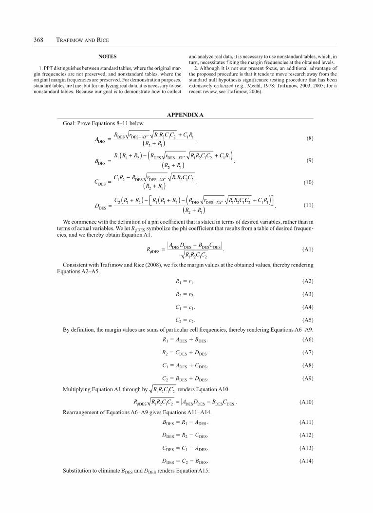
APPENDIX A

Goal: Prove Equations 8–11 below.

A

R r R R C C C R

R RXX

DESDES DES 1 2 1 2 1 1

2 1

.

(8)

B

R R R R r R R C C C R

RXX

DESDES DES1 1 2 1 2 1 2 1 1

22 1R.

(9)

C

C R R r R R C C

R RXX

DESDES DES1 2 1 2 1 2

2 1

.

(10)

D

C R R R R R R r R R CXX

DES

DES DES2 1 2 1 1 2 1 2 1CC C R

R R2 1 1

2 1

.

(11)

We commence with the definition of a phi coefficient that is stated in terms of desired variables, rather than in terms of actual variables. We let R DES symbolize the phi coefficient that results from a table of desired frequen-cies, and we thereby obtain Equation A1.

R

A D B C

R R C CDES

DES DES DES DES

1 2 1 2

.

(A1)

Consistent with Trafimow and Rice (2008), we fix the margin values at the obtained values, thereby rendering Equations A2–A5.

R1 r1. (A2)

R2 r2. (A3)

C1 c1. (A4)

C2 c2. (A5)

By definition, the margin values are sums of particular cell frequencies, thereby rendering Equations A6–A9.

R1 ADES BDES. (A6)

R2 CDES DDES. (A7)

C1 ADES CDES. (A8)

C2 BDES DDES. (A9)

Multiplying Equation A1 through by R1R2C1C2 renders Equation A10.

R R R C C A D B CDES DES DES DES DES1 2 1 2 . (A10)

Rearrangement of Equations A6–A9 gives Equations A11–A14.

BDES R1 ADES. (A11)

DDES R2 CDES. (A12)

CDES C1 ADES. (A13)

DDES C2 BDES. (A14)

Substitution to eliminate BDES and DDES renders Equation A15.

PPT METHODOLOGY 369

APPENDIX A (Continued)

R R R C C A R C C R ADES DES DES DES DES1 2 1 2 2 1 . (A15)

More substitution, to eliminate CDES, leaves an equation with only one unknown (ADES), and renders Equation A16.

R R R C C A R C A C ADES DES DES DE1 2 1 2 2 1 1 SS DESR A1 . (A16)

Expansion of Equation A16 renders Equation A17.

R R R C C R A C A A C R C ADES DES DES DES D1 2 1 2 2 12

1 1 1 EES DES DESR A A12 . (A17)

Collecting the terms renders Equation A18.

R R R C C R A C R R ADES DES DES1 2 1 2 2 1 1 1 . (A18)

It is now time to isolate ADES. We start by switching the term that does not contain ADES to the opposite side of the equation, thereby rendering Equation A19.

R R R C C C R R A R ADES DES DES1 2 1 2 1 1 2 1 . (A19)

Factoring renders Equation A20.

R R R C C C R A R RDES DES1 2 1 2 1 1 2 1 . (A20)

Dividing Equation A20 through by (R2 R1) renders Equation A21.

R R R C C C R

R RADES

DES1 2 1 2 1 1

2 1

.

(A21)

Equation A22 is a restatement of Equation A21. Also, Equations A23–A25 can be obtained by subtraction from the margin frequencies (see Equations A11–A14).

A

R R R C C C R

R RDESDES 1 2 1 2 1 1

2 1

.

(A22)

B

R R R R R R C C C R

R RDESDES1 1 2 1 2 1 2 1 1

2 1

.

(A23)

C

C R R R R C C

R RDESDES1 2 1 2 1 2

2 1

.

(A24)

D

C R R R R R R R R C C C RDES

DES2 1 2 1 1 2 1 2 1 2 1 1

R R2 1

.

(A25)

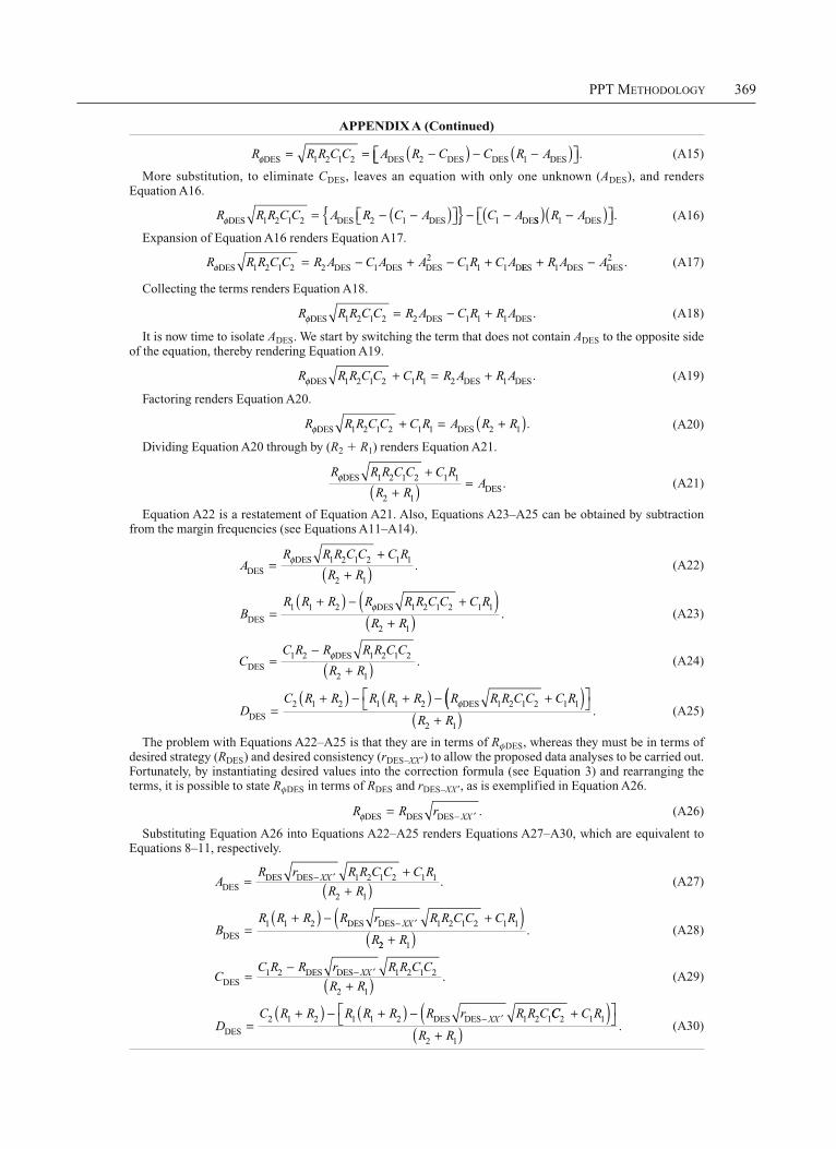
The problem with Equations A22–A25 is that they are in terms of R DES, whereas they must be in terms of desired strategy (RDES) and desired consistency (rDES–XX ) to allow the proposed data analyses to be carried out. Fortunately, by instantiating desired values into the correction formula (see Equation 3) and rearranging the terms, it is possible to state R DES in terms of RDES and rDES–XX , as is exemplified in Equation A26.

R R r XXDES DES DES . (A26)

Substituting Equation A26 into Equations A22–A25 renders Equations A27–A30, which are equivalent to Equations 8–11, respectively.

A

R r R R C C C R

R RXX

DESDES DES 1 2 1 2 1 1

2 1

.

(A27)

B

R R R R r R R C C C R

RXX

DESDES DES1 1 2 1 2 1 2 1 1

22 1R.

(A28)

C

C R R r R R C C

R RXX

DESDES DES1 2 1 2 1 2

2 1

.

(A29)

D

C R R R R R R r R R CXX

DES

DES DES2 1 2 1 1 2 1 2 1CC C R

R R2 1 1

2 1

.

(A30)

370 TRAFIMOW AND RICE

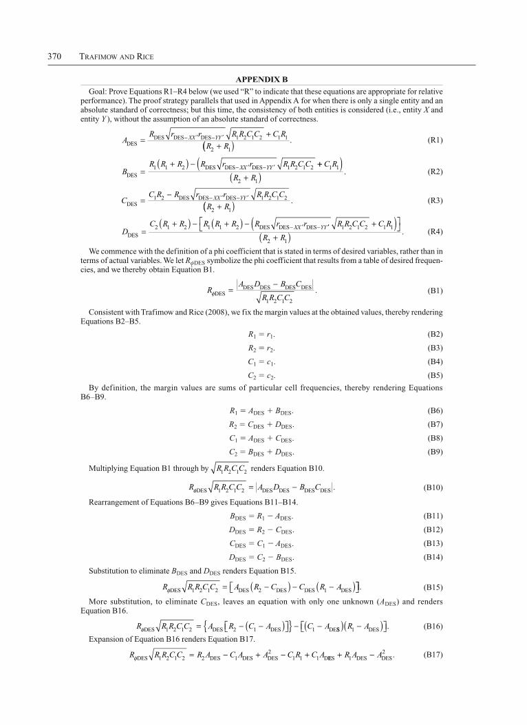
APPENDIX B

Goal: Prove Equations R1–R4 below (we used “R” to indicate that these equations are appropriate for relative performance). The proof strategy parallels that used in Appendix A for when there is only a single entity and an absolute standard of correctness; but this time, the consistency of both entities is considered (i.e., entity X and entity Y ), without the assumption of an absolute standard of correctness.

A

R r r R R C C C R

R RXX YY

DESDES DES DES 1 2 1 2 1 1

2 1

.

(R1)

B

R R R R r r R R C CXX YYDES

DES DES DES1 1 2 1 2 1 2 C R

R R1 1

2 1

.

(R2)

C

C R R r r R R C C

R RXX YY

DESDES DES DES1 2 1 2 1 2

2 1

.

(R3)

D

C R R R R R R r rXX Y

DES

DES DES DES2 1 2 1 1 2 Y R R C C C R

R R1 2 1 2 1 1

2 1

.

(R4)

We commence with the definition of a phi coefficient that is stated in terms of desired variables, rather than in terms of actual variables. We let R DES symbolize the phi coefficient that results from a table of desired frequen-cies, and we thereby obtain Equation B1.

R

A D B C

R R C CDES

DES DES DES DES

1 2 1 2

.

(B1)

Consistent with Trafimow and Rice (2008), we fix the margin values at the obtained values, thereby rendering Equations B2–B5.

R1 r1. (B2)

R2 r2. (B3)

C1 c1. (B4)

C2 c2. (B5)

By definition, the margin values are sums of particular cell frequencies, thereby rendering Equations B6–B9.

R1 ADES BDES. (B6)

R2 CDES DDES. (B7)

C1 ADES CDES. (B8)

C2 BDES DDES. (B9)

Multiplying Equation B1 through by R1R2C1C2 renders Equation B10.

R R R C C A D B CDES DES DES DES DES1 2 1 2 . (B10)

Rearrangement of Equations B6–B9 gives Equations B11–B14.

BDES R1 ADES. (B11)

DDES R2 CDES. (B12)

CDES C1 ADES. (B13)

DDES C2 BDES. (B14)

Substitution to eliminate BDES and DDES renders Equation B15.

R R R C C A R C C R ADES DES DES DES DES1 2 1 2 2 1 . (B15)

More substitution, to eliminate CDES, leaves an equation with only one unknown (ADES) and renders Equation B16.

R R R C C A R C A C ADES DES DES 1 DE1 2 1 2 2 1 SS DESR A1 . (B16)

Expansion of Equation B16 renders Equation B17.

R R R C C R A C A A C R C ADES DES DES DES D1 2 1 2 2 12

1 1 1 EES DES DESR A A12 . (B17)

PPT METHODOLOGY 371

APPENDIX B (Continued)

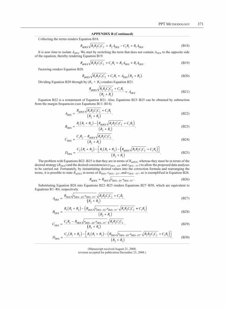
Collecting the terms renders Equation B18.

R R R C C R A C R R ADES DES DES1 2 1 2 2 1 1 1 . (B18)

It is now time to isolate ADES. We start by switching the term that does not contain ADES to the opposite side of the equation, thereby rendering Equation B19.

R R R C C C R R A R ADES DES DES1 2 1 2 1 1 2 1 . (B19)

Factoring renders Equation B20.

R R R C C C R A R RDES DES1 2 1 2 1 1 2 1 . (B20)

Dividing Equation B20 through by (R2 R1) renders Equation B21.

R R R C C C R

R RADES

DES1 2 1 2 1 1

2 1

.

(B21)

Equation B22 is a restatement of Equation B21. Also, Equations B23–B25 can be obtained by subtraction from the margin frequencies (see Equations B11–B14).

A

R R R C C C R

R RDESDES 1 2 1 2 1 1

2 1

.

(B22)

B

R R R R R R C C C R

R RDESDES1 1 2 1 2 1 2 1 1

2 1

.

(B23)

C

C R R R R C C

R RDESDES1 2 1 2 1 2

2 1

.

(B24)

D

C R R R R R R R R C C C RDES

DES2 1 2 1 1 2 1 2 1 2 1 1

R R2 1

.

(B25)

The problem with Equations B22–B25 is that they are in terms of R DES, whereas they must be in terms of the desired strategy (RDES) and the desired consistencies (rDES XX and rDES YY ) to allow the proposed data analyses to be carried out. Fortunately, by instantiating desired values into the correction formula and rearranging the terms, it is possible to state R DES in terms of RDES, rDES XX , and rDES YY , as is exemplified in Equation B26.

R R r rXX YYDES DES DES DES . (B26)

Substituting Equation B26 into Equations B22–B25 renders Equations B27–B30, which are equivalent to Equations R1–R4, respectively.

A

R r r R R C C C R

R RXX YY

DESDES DES DES 1 2 1 2 1 1

2 1

.

(B27)

B

R R R R r r R R C CXX YYDES

DES DES DES1 1 2 1 2 1 2 C R

R R1 1

2 1

.

(B28)

C

C R R r r R R C C

R RXX YY

DESDES DES DES1 2 1 2 1 2

2 1

.

(B29)

D

C R R R R R R r rXX Y

DES

DES DES DES2 1 2 1 1 2 Y R R C C C R

R R1 2 1 2 1 1

2 1

.

(B30)

(Manuscript received August 21, 2008; revision accepted for publication December 23, 2008.)