Economic Analysis of Ontario’s First Poverty Reduction Strategy

Kyel Governor

Poverty in Canada has become a greater concern among Canadians in recent years with many

Canadians finding it difficult to keep up with the costs of living. In 2011 Canada ranked 24th out of 34 in

lowest poverty rate among Organization for Economic Co-operation and Development (OECD) countries

with a poverty rate of 8.8% according to the after tax Low Income Cut-Off (LICO-AT) poverty line

measure. The average gap between the LICO-AT poverty line and household income below the LICO-

AT is 33% (Citizens of Public Justice, 2012). Therefore a low income family of four living in a city with

a population of more than 500, 000 expected income would be $24,458 which is $12,046 under the

LICO-AT poverty line (Citizens of Public Justice, 2012). Such a high poverty rate and significant depth

of poverty for a country as wealthy as Canada illustrates the lack of social welfare for the poorest

Canadians.

This paper focuses on the problem of poverty in Ontario because it is one of Canada’s strongest

provinces generating 37% of Canada’s Gross Domestic Product (GDP) and approximately 40% of

Canadians live in the province. Poverty has significant efficiency costs in Ontario. The efficiency costs

comprise of both private and social costs (Laurie, 2008). The private costs are the lost potential income

and poverty induced costs that individuals suffer while the social costs are the lost potential tax revenue

and poverty induced costs that the government suffers. The total efficiency cost of poverty in Ontario

considers remedial, intergenerational and opportunity costs and is equal to 5.5% to 6.6% of Ontario’s

GDP. Furthermore living in poverty likely leads to poor health, lower productivity, lower educational

attainment and lower child’s future income thus creating major disparities in opportunities between those

living in poverty and those who are not (Laurie, 2008). Without assistance many living in poverty will

remain in poverty and so will their children.

The provincial government insists that addressing intergenerational poverty is the primary

response to alleviating poverty in Ontario (Ontario). The total efficiency cost of intergenerational poverty

in Ontario is very significant at $4.6 to $5.9 billion annually (Laurie, 2008). Also, the issue is ethically

troubling because a child living in poverty is more likely to be in poverty as an adult than a child who did

not live in poverty. Most will argue that all children should have equal opportunity to attain an adequate

income. Thus Ontario’s first poverty reduction strategy is aimed at addressing child poverty. The paper

will provide economic analysis on policies targeted at reducing child poverty; specifically the Ontario

Child Benefit (OCB) and investment in educational programs.

To assess the economic efficiency of the policies directed to reducing child poverty the paper will

be divided into two major parts. The first will be a cost benefit analysis and the second will be a social

welfare analysis. The costs and benefits of the OCB is influenced by DeSalvo’s report on New York

City’s Mitchell-Lama program, “Benefits and Costs of New York City’s Middle-Income Housing

Program” and assesses how well the grant targets childcare costs through modelling household’s

childcare expenditure versus consumption on all other goods, with adjustments made to account for

differences in utility of two different household types (DeSalvo, 1975). The cost-benefit analysis on

investment in educational programs follows a simple return on investment model. The social welfare

analysis is mainly driven by the research paper “Describing the Distribution of Income: Guidelines for

Effective Analysis” by M.Skuterud, M.Frenette, and P.Poon and evaluates the overall effectiveness of

each policy by looking at the resulting change in poverty rate, poverty gap, and poverty intensity

(Skuterud, Frenette, & Poon, 2004). In the end, whether the child poverty reduction policies are efficient

and effective toward reducing poverty in Ontario will be answered. If this is true, then Ontario’s strategy

for poverty reduction should be intensified and can be considered a successful first-step approach to

reducing poverty.

Background

In 2008 Ontario released its first poverty reduction strategy called ‘Breaking the Cycle’. The

strategy claims that breaking the cycle of intergenerational poverty is the best way to combat poverty. The

aim is to implement policies to reduce child poverty in Ontario by 25% in 5 years, which would take

90,000 children out of poverty (Ontario). The assertion is that society will gain from investments toward

child poverty reduction policies because the future expected cost of poverty will be lower and the

expected return from human resources will be greater while we benefit from improved social welfare.

Two main policies in the strategy are the OCB and investment in education. The OCB is a guaranteed

income, or demogrant, aimed at helping low income families cover childcare costs. The OCB promises up

to $1,310 per child per year and will support 1.3 million children in low income families for a total

investment of $1.3 billion annually (Ontario). Policies to invest in educational programs for low income

children aim to increase the high school graduation rate and the postsecondary attendance rate of low

income children thereby increasing human capital. Increasing the number of Parenting and Family

Literacy Centres, supplying more after school programs and implementing full-day learning for four and

five year olds are examples of educational programs that the strategy outlines (Ontario). These two

policies are the driving force of the poverty reduction strategy and therefore this paper looks to determine

if they are economically efficient and effective.

PART I – Benefits and Costs

Introduction and Definitions

The OCB is a guaranteed income to low income families with children. At earnings of $20,000 or

less per year a family is eligible to receive the full amount of $1,310 per child annually (Ontario). Low

income families earning more than $20,000 annually receive a portion of the benefit as shown in Table 1.

The aim of the OCB is to give financial assistance to children. Figure 1 and Figure 2 show the effect of

OCB on income for an adult working minimum wage with two children and a non-working adult with

two children.

In this paper education will be viewed in terms of human capital. Assume that an additional year

of schooling increases expected earnings and that this can be modelled by the Mincer equation log y = log

y0 + δS +β1X +β2X2 where y is earnings, S is years of schooling, and X is work experience (Lemieux,

2003). For the sake of investigating the return to education for children, work experience is omitted from

this equation leaving log y = log y0 + δS where δ is the rate of return to an additional year of schooling.

Ontario Child Benefit

The Method

To determine the targeting efficiency of the OCB the paper evaluates how much of the OCB the

household spends on childcare versus on all other goods. Household expenditure on children is derived by

maximizing a household’s utility curve subject to a budget constraint. Utility curves are estimated using

OECD equivalence scales. The equivalence scale that is used in this paper is most appropriately restricted

to low income households and assigns 1 for the first adult, 0.4 for each none working adult and 0.3 for

each child (Skuterud, Frenette, & Poon, 2004). However it should be noted that OECD equivalence scales

measure how much more income a household needs due to the addition of another child or adult to be as

well off as before and does not directly measure household childcare spending. Nonetheless it is a strong

estimator of childcare spending for low income households (Sarlo, 2013). A simple Cobb-Douglas utility

function can be easily derived to represent child-consumption preferences modelled as; U(c,x) = cbx

1-b

where c is expenditure on children, x is expenditure on all other goods, and b = 0.3N/1+0.4A+0.3N where

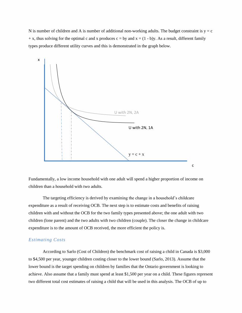
N is number of children and A is number of additional non-working adults. The budget constraint is y = c

+ x, thus solving for the optimal c and x produces c = by and x = (1 - b)y. As a result, different family

types produce different utility curves and this is demonstrated in the graph below.

Fundamentally, a low income household with one adult will spend a higher proportion of income on

children than a household with two adults.

The targeting efficiency is derived by examining the change in a household’s childcare

expenditure as a result of receiving OCB. The next step is to estimate costs and benefits of raising

children with and without the OCB for the two family types presented above; the one adult with two

children (lone parent) and the two adults with two children (couple). The closer the change in childcare

expenditure is to the amount of OCB received, the more efficient the policy is.

Estimating Costs

According to Sarlo (Cost of Children) the benchmark cost of raising a child in Canada is $3,000

to $4,500 per year, younger children costing closer to the lower bound (Sarlo, 2013). Assume that the

lower bound is the target spending on children by families that the Ontario government is looking to

achieve. Also assume that a family must spend at least $1,500 per year on a child. These figures represent

two different total cost estimates of raising a child that will be used in this analysis. The OCB of up to

c

x

U with 2N, 1A

U with 2N, 2A

y = c + x

$1,310 per child aims to subsidize childcare cost and so the total cost of raising a child can be broken

down into two parts; the household contribution and the non-household contribution.

Estimating Benefits

The direct benefit associated with the OCB is the change in child expenditure as a result of the

subsidy. The indirect benefits are positive externalities created by the remainder of the OCB that does not

contribute to childcare. Therefore, total benefits will be the sum of direct and indirect benefits generated

by the OCB.

The model estimates that, per child, only 18.75% of the OCB is used by the lone parent on

childcare and 15% of the OCB is used by the couple. Therefore the net direct benefit is $245.63 and

$196.50 respectively. Subtracting net benefits from the OCB there is a misallocation of $1064.37 for the

lone parent and $1113.5 for the couple. However for incomes below $8,000 and $10,000, OCB included,

none of the OCB received is contributed to household’s child expenditure, the net direct benefit is $0 and

the misallocation is equal to the OCB.

Aggregate Effects

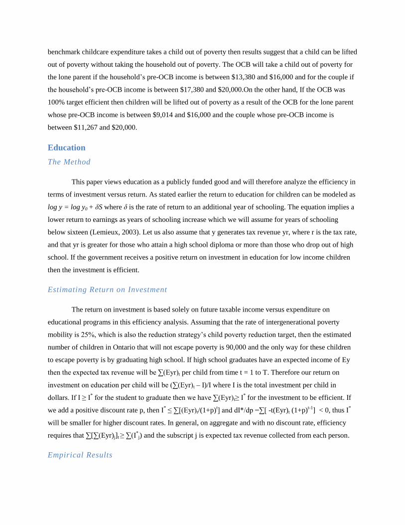
The graph below illustrates the change in childcare expenditure for the lone parent. After

receiving OCB, for income above $8,000 y1 moves to y

1ocb, and for incomes below $8,000 y

0 moves to

y0ocb. The hard dashed line shows that the household must spend at least $3,000 on childcare. The

resulting utility curves of the lone parent are shown for each scenario.

Lone parent (1A, 2N)

Since only a portion of the subsidy goes directly to childcare the OCB can be deemed inefficient.

It can be argued that, if the child is as well or better off with the predicted allocation of the OCB

versus if all of the OCB were to be spent on the child then the policy can be seen as efficient. This

requires the child’s utility function which is beyond the scope of this paper. In speculation, assuming that

child expenditure has a greater impact on the child’s utility than household expenditure on all other goods

then the OCB is more efficient for the lone parent than the couple.

Results

The income levels that are necessary to achieve the government’s desired expenditure on children

are calculated for the two family types of interest. The utility model predicts that the lone parent must

have an income of at least $16,000 and the couple must have an income of at least $20,000. Furthermore,

spending between child expenditure and on all other goods is sub-optimal for the lone parent whose

income is below $8,000 and for the couple whose income is below $10,000. If by achieving the

$c

$x

$3000

u1

ocb

u1

u0

ocb

u0

$2

,620

$491.20

benchmark childcare expenditure takes a child out of poverty then results suggest that a child can be lifted

out of poverty without taking the household out of poverty. The OCB will take a child out of poverty for

the lone parent if the household’s pre-OCB income is between $13,380 and $16,000 and for the couple if

the household’s pre-OCB income is between $17,380 and $20,000.On the other hand, If the OCB was

100% target efficient then children will be lifted out of poverty as a result of the OCB for the lone parent

whose pre-OCB income is between $9,014 and $16,000 and the couple whose pre-OCB income is

between $11,267 and $20,000.

Education

The Method

This paper views education as a publicly funded good and will therefore analyze the efficiency in

terms of investment versus return. As stated earlier the return to education for children can be modeled as

log y = log y0 + δS where δ is the rate of return to an additional year of schooling. The equation implies a

lower return to earnings as years of schooling increase which we will assume for years of schooling

below sixteen (Lemieux, 2003). Let us also assume that y generates tax revenue yr, where r is the tax rate,

and that yr is greater for those who attain a high school diploma or more than those who drop out of high

school. If the government receives a positive return on investment in education for low income children

then the investment is efficient.

Estimating Return on Investment

The return on investment is based solely on future taxable income versus expenditure on

educational programs in this efficiency analysis. Assuming that the rate of intergenerational poverty

mobility is 25%, which is also the reduction strategy’s child poverty reduction target, then the estimated

number of children in Ontario that will not escape poverty is 90,000 and the only way for these children

to escape poverty is by graduating high school. If high school graduates have an expected income of Ey

then the expected tax revenue will be ∑(Eyr)t per child from time t = 1 to T. Therefore our return on

investment on education per child will be (∑(Eyr)t – I)/I where I is the total investment per child in

dollars. If I ≥ I* for the student to graduate then we have ∑(Eyr)t≥ I

* for the investment to be efficient. If

we add a positive discount rate p, then I* ≤ ∑[(Eyr)t/(1+p)

t] and dI*/dp =∑[ -t(Eyr)t (1+p)

t-1] < 0, thus I

*

will be smaller for higher discount rates. In general, on aggregate and with no discount rate, efficiency

requires that ∑[∑(Eyr)j]t ≥ ∑(I*j) and the subscript j is expected tax revenue collected from each person.

Empirical Results

The program Pathways to Education, directed to improving high school graduation rates in low

income neighbourhoods, was introduced in Regent Park which has the highest poverty rate in the Greater

Toronto Area. Before the program the neighborhood had a dropout rate of 56% which is 45% higher than

Toronto’s highest income neighborhood, and post-secondary enrolment was 20%. The program has

decreased the dropout rate to 10% and increased post-secondary enrolment to 80% in Regent Park

(Laurie, 2008).

By investing in a program like Pathways to Education for the 90,000 children we can assume that

this sample’s future income distribution will represent the income distribution of the population (Laurie,

2008). If so then the gross benefit from the program is the expected tax revenue generated from the

sample’s new income distribution minus the tax revenue generated if the sample remained in poverty. By

subtracting the average tax revenue per person in poverty from the average tax revenue per person in

Ontario in 2006 and multiplying by 90,000, it is estimated that the government can expect an increase in

tax revenue of at least $1.835 billion dollars per year from the program in 2007 dollars. The program’s

cost per child is roughly $3,500 annually and after adding the marginal schooling cost per child the total

cost is $7,000 per child each year (Laurie, 2008). On aggregate the necessary yearly investment is $630

million. Assuming that the government receives at least 4 years of the expected tax revenue and the

investment length is also 4 years then the yearly net benefit of the program is $1.205 billion and the return

on investment is 1.91. The Boston Consulting Group cost benefit analysis on Pathways to Education

estimates a 1.8 benefit to cost ratio (Laurie, 2008). The group measures the present value of social

benefits at $50,000 per student and the cost at $28,000 per student resulting in a return on investment of

approximately 0.8. Since the return on investment is positive the policy to invest in educational programs

such as Pathways to Education is efficient.

PART II – Social Welfare

Introduction and Definitions

The impact that the OCB and investment in educational programs for low income children have

on social welfare in Ontario is important when measuring their effectiveness. By using income as an

indicator for well-being we can measure the effectiveness by analyzing how much the policies reduce the

rate of poverty and the poverty gap.

The poverty line that will be used in this analysis is the same measure used in the reduction

strategy which is the Low Income Measure after tax (LIM-AT) calculated as 50% of median income after

tax. The rate of poverty is the number of persons with an after tax income below the LIM-AT divided by

the population. Lastly, the poverty gap is calculated as the difference between the LIM-AT and the

average of the after tax incomes of those under the LIM-AT, divided by the LIM-AT (Skuterud, Frenette,

& Poon, 2004). As mentioned before the strategy’s objective is to take 90,000 children out of poverty so

if the poverty rate becomes zero for the 90, 000 children as a result of the policies then the policies are

100% effective. Thus effectiveness is measured by number of children out of poverty divided by 90,000.

The change in the poverty gap can be seen as a secondary measure of effectiveness since reducing the rate

of poverty but increasing the poverty gap will have a negative effect on the social welfare of the poor and

an ambiguous change in overall social welfare. In other words, the change in low income intensity must

be considered. The low income intensity is the product of the poverty rate, the poverty gap and 1 plus the

Gini coefficient of the distribution of low-income gaps in the population (where everybody above the

LIM-AT is assigned a gap of 0 instead of something positive) (Skuterud, Frenette, & Poon, 2004). Either

zero or a negative change in the low income intensity is necessary for a policy to be considered effective

in reducing child poverty.

Ontario Child Benefit and the Poverty Gap

The OCB is a guaranteed income to low income families with children. The benefit has a claw

back so that families with higher incomes receive less OCB (See Table 1). Therefore the OCB is not very

effective since very few families will be lifted out of poverty as a result of receiving OCB; however it

does reduce the poverty gap. The overall effectiveness of the OCB can be measured for the two family

types of interest which are the lone parent and the couple, both with two children. Their LIM-AT in 2007

are $30,754 and $35,512 respectively. The average poverty gaps for each family type are 29% and 24.9%

therefore the average low incomes are $21,835 and $26,669 (Statistics Canada). If the claw back is

neglected then every family will receive $1,310 per child. As a result, the new average income for the

lone parent is $24,455 and the poverty gap becomes 20.5%, and the new average income for the couple is

$29,289 and the poverty gap becomes 17.5%. The OCB without claw back will reduce the poverty gap by

8.5 percentage points for the lone parent and 7.4 percentage points for the couple. Since at least 50% of

families have an after tax income below $20,000 in each of the family types then the poverty gap is

reduced by at least 4.25 percentage points for the lone parent and 3.7 percentage points for the couple

(Statistics Canada, 2013). The OCB is very ineffective in reducing poverty rates but is somewhat

effective in reducing the poverty gap and thus also reduces the low income intensity.

Education and the Poverty Rate

Investing in educational programs for at-risk low income children can lead to a reduction in the

future poverty rate and the future poverty gap. With an intergenerational poverty mobility of 25% there

will be an expected 90,000 children remaining in poverty as adults however if these children are targeted

and placed in educational programs such as Pathways to Education, fewer children will be expected to

remain in poverty as adults (Wagmiller Jr. & Adelman, 2009). The percentage of the children expected to

remain in poverty can be estimated using the population’s after tax income distribution and the Pathways

to Education 10% dropout rate and 80% postsecondary participation rate. Also the LIM-AT in 2010 is

$19,161 so all incomes below $20,000 will be considered below the LIM-AT for ease of calculation

(Statistics Canada, 2013). The program predicts out of the 90,000 children, 9,000 will have no high

school diploma, 16,200 will have a high school diploma and 64,800 will have more than a high school

diploma. The income distributions predict that out of the 9,000 children, 5,588 will be below the LIM-

AT; out of the 16,200, 7,940 will be below the LIM-AT; and out of the 64,800, 18,392 will be below the

LIM-AT (Statistics Canada, 2011). The expected poverty rate out of the 90,000 is 35.5% and therefore the

programs will have an effectiveness of 64.5% in reducing the child poverty rate if precisely targeted. If

only half of the children are correctly targeted then the programs are 32.25% effective in reducing the

child poverty rate. The poverty gap is expected to change since some of the children will have higher

expected incomes but not enough to escape poverty. There will be a negative change in the low income

intensity since there is a negative change in the poverty rate and in the poverty gap.

Conclusion

Summary

Breaking the cycle of intergenerational poverty is a worthy first step approach to reducing

poverty in Ontario given its moral imperatives and strong economic incentives. To address child poverty,

the Ontario government put forth a poverty reduction strategy in 2008 with the goal to reduce child

poverty by 25% in five years. This paper focused on analyzing the efficiency and effectiveness of the two

main policies outlined in the plan, the Ontario Child Benefit and investment in educational programs. The

Ontario Child Benefit aims to support low income families in covering childcare costs. The targeting

efficiency of the policy is very low with only a small fraction of the grant spent on childcare by

households however the OCB is more efficient for single parent families than for two parent families. If

the government wished to achieve the benchmark spending on childcare by households, only a few

households will do so as a result of receiving OCB. Although the OCB lacks efficiency, it has a positive

effect on social welfare because it reduces poverty intensity. Investment in educational programs is aimed

at improving human capital among children giving them the opportunity to escape poverty as adults. The

benefits from investing in educational programs such as Pathways to Education overcome the costs and

show a positive return on investment showing that such programs are efficient. The resulting social

welfare from such educational programs is improved because the future poverty rate and gap is reduced

and thus the future poverty intensity reduces as well.

Limitations

This paper faces several limitations. Starting with the OCB analysis, childcare expenditure is not

directly measured and is inferred from the OECD equivalence scale. To derive a direct household

spending on childcare function is not plausible however the equivalence scale used provides a good

estimate in context of low income families childcare spending. Furthermore the benchmark and minimum

cost of a child is based on a budget approach and suffers from a degree of subjectivity (Sarlo, 2013). The

inability to derive a child’s utility function also hinders the paper’s ability to accurately assess the benefits

associated with the OCB.

The limitations associated with the investment in educational programs analysis are that the

benefits occur in the long run and so a degree of uncertainty should be introduced, such as chances of

emigration and death. However the paper likely undershoots the benefits of investment since it only

accounts for future tax revenue.

In general, the analysis does not take into account how the policies affect special demographics

such as single mothers, aboriginals, crown wards, children with disabilities, and recent immigrants. Lastly

the paper fails to account for the benefits, other than the costs of the policies, associated with not

implementing the policies which likely underestimate the costs of the policies.

Alternative Policies

There are three types of policies that policy makers can choose from to assist low income families

with childcare costs; direct money transfers, subsidizing child inputs, and directly providing child inputs.

Direct money transfers are very inefficient at targeting childcare costs. The OCB is a direct

money transfer and shows that only a small portion of the money is spent on childcare by the household.

A direct money transfer results in only an income effect and households increase consumption of both

childcare and all other goods, resulting in an unambiguous increase in utility, but do not change spending

patterns.

Subsidizing child inputs is more efficient at targeting childcare costs than a direct money transfer

because the income effect will be smaller and the substitution effect will lead to an increase in the amount

spent on childcare by households. To illustrate this if the original budget line is y = c + x, subsidizing

child inputs by 20% will lead to a new budget line, y = 0.8c + x. Thus the new optimal expenditure on

childcare is c = yb/0.8 which is greater than c = yb. So spending patterns change in favour of childcare

and utility is unambiguously increased. The drawback however is that based on the equivalent value

argument subsidizing child inputs leads to an efficiency loss not experienced by direct money transfers.

Directly providing child inputs is the most efficient at targeting childcare costs but crowds out

household’s spending on childcare. This is because as more inputs are provided, household’s preferences

change and less weight is put on the child thus the utility curve becomes less sensitive to childcare

spending. To illustrate this if the original weight put on a child is 0.3 according to the equivalence scale,

providing more child inputs leads to a new weight put on a child that is less than 0.3. Therefore the new

utility curve will reflect this and a lower percentage of income will be spent on childcare expenditure

resulting in a substitution effect away from childcare spending and into consumption of all other goods.

Educational programs such as Pathways to Education do not directly impact the household and

only provides direct benefits to the child. However after school programs and implementing full day

learning for four and five year olds can allow parents to work longer hours and increase household

income.

Closing Remarks

Investment in education proves to be the soundest policy in the poverty reduction strategy. If

targeted to the most at risk youth, it can be extremely effective and efficient at reducing child poverty

rates. A stronger and more efficient educational system will generate the greatest economic return in

terms of poverty rate reduction (Laurie, 2008). Providing low income families the means to take care of

their children is essential for healthy development and success in school. Children will be less productive

due to inadequate childcare and thus lower the returns of investment in education. The OCB is very

inefficient at providing childcare. A better policy is to subsidize essential child inputs while providing

child inputs that are not essential to childcare but improves the child’s productivity, such as books,

laptops, tutoring or even future assets. A stronger policy than that is to encourage those who are very well

off to assist the poor. “But if anyone has the world's goods and sees his brother in need, yet closes his

heart against him, how does God's love abide in him? Little children, let us not love in word or talk but in

deed and in truth.”(1 John 3:17-18, ESV) There is truth to these words from the Gospel; some close their

hearts to those in need but many do not know or see those who are in need. Creating a better market for

philanthropy and limiting government intervention is the best economic policy to combat poverty in

Ontario. It is the most efficient as a result of less deadweight loss generated by government intervention,

and it promotes economic growth as a result of an emerging market and an increase in productivity from

the poorest in the province.

Bibliography Citizens of Public Justice. (2012). Poverty Trends Scorecard.

DeSalvo, J. S. (1975). Benefits and Costs of NY City's Middle Income Housing Project. Journal of

Political Economy, 791-805.

Laurie, N. (2008). The Cost of Poverty. Toronto: Ontario Association of Food Banks.

Ontario. (n.d.). Breaking the Cycle. Ontario's Poverty Reduction Strategy.

Sarlo, C. (2013). The Cost of Raising Children. Fraser Institute.

Skuterud, M., Frenette, M., & Poon, P. (2004). Describing the Distribution of Income: Guidelines for

Effective Analysis. Ottawa: Statistics Canada.

Statistics Canada. (2013, 05 02). Low Income Cut-offs. Retrieved from

http://www.statcan.gc.ca/pub/75f0002m/2012002/lico-sfr-eng.htm

Statistics Canada. (2013, 06 07). Persons in low income after tax. Retrieved from

http://www.statcan.gc.ca/tables-tableaux/sum-som/l01/cst01/famil19a-eng.htm

Statistics Canada. (n.d.). Table 202-0804 - Persons in low income, by economic family type, annual.

Retrieved March 09, 2015

Wagmiller Jr., R., & Adelman, R. (2009). Childhood and Intergenerational Poverty. National Center for

Children in Poverty.

Appendix

Table 1- Ontario Child Benefits- Monthly

# of Children $20,000 $25,000 $30,000

1 $109.16 $75.83 $42.50

2 $218.33 $185.00 $151.66

3 $327.50 $294.16 $260.83

4 $436.66 $403.33 $370.00

Figure 1-Working Lone Parent with Two Children

Figure 2 – Non-Working Lone Parent with Two Children

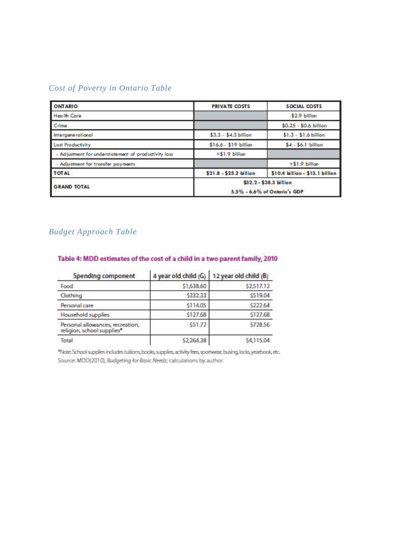
Cost of Poverty in Ontario Table

Budget Approach Table

Targeting Efficiency of OCB Table

% of OCB Spent on Childcare (per

child)

Income at Minimum Child Expenditure

Income at Benchmark Child Expenditure

# of Children

Lone Parent Couple Lone Parent Couple Lone

Parent Couple

1 23% 17.65% $

6,521.74 $

8,498.58 $

13,043.48 $

16,997.16

2 18.75% 15% $

8,000.00 $

10,000.00 $

16,000.00 $

20,000.00

3 15.79% 13.04% $

9,499.68 $

11,503.07 $

18,999.36 $

23,006.14

Income Where OCB Helps Achieve Benchmark Child

Expenditure

Income Where OCB at 100% Target Efficiency Helps Achieve Benchmark

Child Expenditure

# of Children

Lone Parent

Couple Lone Parent Couple

1 $

11,733.48 $

15,687.16 $

7,347.83 $

9,575.08

2 $

13,380.00 $

17,380.00 $

9,013.34 $

11,266.67

3 $

15,069.36 $

19,076.14 $

10,702.98 $

12,960.13

Policy and Household Interactions

Direct Money

Transfer Subsidized

Child Inputs Provided Child

Inputs Pathways to

Education

After School/Early

Child Learning Programs

Child Expenditure Increase Increase Decrease Same Increase

All Other Goods Increase Same Increase Same Increase

Substitution Effect

No Yes Yes No No

Income Effect Yes Yes No No Yes

Utility Increase Increase Curve Changes Same Increase