poverty in the regions of the...
TRANSCRIPT

Dorota Weziak-Bialowolska Lewis Dijkstra
Regional Human Poverty Index Poverty in the regions of the European
2 0 1 4
Report EUR 26792 EN

European Commission
Joint Research Centre
Contact information
Dorota Weziak-Bialowolska
Address: Joint Research Centre, Via Enrico Fermi 2749, TP 361, 21027 Ispra (VA), Italy
E-mail: [email protected]
Tel.: +39 0332 78 9760
https://ec.europa.eu/jrc
Legal Notice
This publication is a Science and Policy Report by the Joint Research Centre, the European Commission’s in-house
science service. It aims to provide evidence-based scientific support to the European policy-making process. The
scientific output expressed does not imply a policy position of the European Commission. Neither the European
Commission nor any person acting on behalf of the Commission is responsible for the use which might be made
of this publication.
The geographic borders are purely a graphical representation and are only intended to be indicative.
The boundaries do not necessarily reflect the official position of the European Commission.
JRC90975
EUR 26792 EN
ISBN 978-92-79-39642-7 (PDF)
ISBN 978-92-79-39643-4 (print)
ISSN 1831-9424 (online)
ISSN 1018-5593 (print)
doi: 10.2788/10063
Luxembourg: Publications Office of the European Union, 2014
© European Union, 2014
Reproduction is authorised provided the source is acknowledged.
Abstract
We measure area-specific poverty in the European Union (EU) at the second level of the nomenclature of
territorial units for statistics (NUTS 2). We construct the regional human poverty index (RHPI), which comprises
four dimensions: social exclusion, knowledge, a decent standard of living, and a long and healthy life. The RHPI
provides information regarding the relative standing of a given country with respect to the level of poverty but
also shows the variability of poverty within a country with respect to NUTS 2.
The RHPI is computed for all NUTS 2 regions in 28 EU countries. Our results show that the scale of poverty differs
considerably within the EU countries, with RHPI scores ranging between 9.23 for Prague and more than 65 for
Bulgarian Yugoiztochen and Severozapaden. We also find that substantial differences in levels of poverty between
regions are present in all of the EU countries. The only exceptions to this finding are small EU countries where
neither NUTS 1 nor NUTS 2 regions exist.
Our results also show that, in general, in NUTS 2 regions comprising a capital, the poverty level is lower than the
country average. The only exceptions are Vienna, Brussels, and Berlin, where poverty measured by the RHPI is
higher than the country average. By contrast, Bucharest, Sofia, Bratislava, Prague, Budapest, and Madrid exhibit
decisively lower levels of poverty than their country averages.

3
Executive summary We measure area-specific poverty in the European Union (EU) at the second level of the
nomenclature of territorial units for statistics (NUTS 2). We construct the regional human poverty
index (RHPI), which comprises four dimensions: social exclusion, knowledge, a decent standard of
living, and a long and healthy life. The RHPI provides information regarding the relative standing of
a given country with respect to the level of poverty but also shows the variability of poverty within a
country with respect to NUTS 2.
The approach we propose has four properties. (1) Because the RHPI comprises only six indicators it
is relatively simple to be replicated in subsequent years. (2) The RHPI provides information about
the absolute magnitude of poverty experienced by Europeans in a given country and provides
information about the relative standing of the country. (3) The RHPI shows the variability of
poverty within a country with respect to NUTS 2. (4) The RHPI shows satisfactory statistical
coherence confirmed by the results of correlation analysis and principal component analysis. As
confirmed by uncertainty analysis, the RHPI also shows satisfactory robustness to the normative
assumptions made during the construction process.
The RHPI also has some limitations. First, the conceptual model of the RHPI relies mostly on the
conceptualisation of the poverty index proposed by the United Nations (UN) and data availability.
Second, although research on poverty has developed rapidly in recent years, it has failed to establish
the relative importance of poverty dimensions and thus guide us in establishing aggregation weights.
This failure has resulted in a necessity to formulate certain a priori assumptions. Third, all indicators
we proposed are of objective nature, which may influence the results and final conclusions.
However, this is intentional and reflects the best approach that is achievable (due to lack of
disaggregated at the NUTS 2 level subjective indicators) in order to measure poverty in the NUTS 2
regions. Fourth, in our computations percentage of population below the income poverty line in
NUTS 2 regions are calculated using national poverty lines and without taking into account social
transfers in kind. Regarding the social transfer in kind, without this type of adjustment household
income is generally underestimated in countries with extensive public services, like in the Nordic
member states, and overestimated in those where households have to pay for most of these services
(Annoni et al., 2012; EC, 2010). However, disaggregated at the NUTS 2 level data with this respect
are not available, therefore our approach is the best achievable. Then, the national, instead of the

4
regional, poverty lines are applied to highlight the differences between regions within the same
country, as suggested by Betti at al. (2012).
The RHPI is computed for all NUTS 2 regions in 28 EU countries. Our results show that the scale
of poverty differs considerably within the EU countries, with RHPI scores ranging between 9.23 for
Prague and more than 65 for Bulgarian Yugoiztochen and Severozapaden. We also find that
substantial differences in levels of poverty between regions are present in all of the EU countries.
The only exceptions to this finding are small EU countries where neither NUTS 1 nor NUTS 2
regions exist.
Our results also show that, in general, in NUTS 2 regions comprising a capital, the poverty level is
lower than the country average. The only exceptions are Vienna, Brussels, and Berlin, where poverty
measured by the RHPI is higher than the country average. By contrast, Bucharest, Sofia, Bratislava,
Prague, Budapest, and Madrid exhibit decisively lower levels of poverty than their country averages.

5
Contents
1. Introduction ........................................................................................................................................... 6
2. Concept of poverty ................................................................................................................................ 6
3. Human Poverty Index by the United Nations ........................................................................................ 9
4. Conceptualisation of the Regional Human Poverty Index ..................................................................... 10
5. Methods ............................................................................................................................................... 11
6. Spatial distribution of the RHPI ........................................................................................................... 13
7. Results from uncertainty analysis .......................................................................................................... 16
8. Conclusions ......................................................................................................................................... 18
References.................................................................................................................................................... 21
Appendix ..................................................................................................................................................... 24

6
1. Introduction
In 2012, 124.5 million people, or 24.8 % of the European Union (EU) population, were at risk of
poverty or social exclusion, compared with 24.3 % in 2011. These numbers change considerably
when poverty is analysed between countries, age groups, and genders and especially when the sub-
national dimension is taken into account. However, information about the distribution of poverty at
the sub-national level is still limited, which seems surprising because the EU regions, not countries,
are the key focus of the European Union's regional policy (Becker, Egger, & von Ehrlich, 2010).
Local differences in poverty are essential to adequately targeting policies, alleviating the causes of
poverty, and mitigating the consequences of poverty.
The measure of poverty officially used in the EU, the ‘at risk of poverty or social exclusion’
(AROPE) rate, combines both income and non-income indicators. It is reported not only at the
country level but also for different levels of the nomenclature of territorial units for statistics (NUTS)
and for areas differently defined with respect to population density. Nevertheless, the AROPE rate
is not reported consistently for all countries. Namely, sub-national estimates of the AROPE rate are
not available for several large countries, including Germany and the United Kingdom. With this
knowledge, it seems reasonable to provide a composite measure of poverty that, next to the AROPE
rate, will enable better identification of NUTS 2 regions where aid is most needed.
This study comprises six sections. First, we present the concept of poverty with a focus on the
multidimensional measurement. Second, we shortly describe the Human Poverty Index proposed by
the United Nations. Third, the conceptualisation of our approach to poverty measurement is
discussed. Fourth, the methods used to construct a composite indicator of poverty are presented.
The results section follows, and the final section concludes the paper.
2. Concept of poverty
The standard of people’s lives both in relative terms, compared to other people in society, and in
absolute terms, whether they enjoy life’s basic necessities, is a reflection of whether people live in
poverty (Callander, Schofield, & Shrestha, 2012). However, the notion of poverty is understood
differently in different contexts. According to Wagle (2008) and Saunders (2005), there are three

7
main approaches in the conceptualisation and operationalisation of poverty: (1) economic well-
being, (2) capability and (3) social inclusion.
The concept of economic well-being links poverty to economic deprivation, which, in turn, relates
to material aspects and physical quality of life or welfare (Boulanger, Lefin, Bauler, & Prignot, 2009;
Wagle, 2008). The capability approach proposed by Sen (1993) expands the notion of poverty from
welfare, consumption and income to broader concepts such as freedom and well-being. Poverty is
understood as the deprivation of capabilities and functionings. Capabilities are the things that a
person is able to do or enable her to lead the life she currently has. Functionings represent
achievements that a person is capable of realising. The third approach, which is based on social
inclusion, is described as the opposite of social exclusion. Social exclusion relates to a state or
situation and stems from the process of systematic isolation, rejection, humiliation, lack of social
support, and denial of participation (Wagle, 2008). It focuses on deficiencies, whereas the capability
approach focuses on possibilities and abilities. The last two approaches expand the notion of
poverty from a purely economic perspective to a more sociological one.
Hagenaars and de Vos (1988) report that three types of poverty can be distinguished:
absolute – meaning that poverty entails having less than an objectively defined, absolute
minimum,
relative – meaning that poverty entails having less than others in society, and
self-assessed – meaning that poverty is a feeling that you do not have enough to get along.
Depending on the type of definition, different indicators are chosen. They can be classified generally
as income and non-income related. Because the choice of definition and thus indicators affect the
results, the multidimensional approach to poverty conceptualisation and operationalisation seems to
be reasonable. There are numerous proponents of such an approach, including Alkire and
Foster(2011a, 2011b), Alkire and Santos (2013), Antony and Visweswara Rao (2007), Bellani (2012),
Betti, Gagliardi, Lemmi, and Verma (2012), Ravallion (2011) and Wagle (2008). In their studies, not
only does the concept of poverty have numerous dimensions but its measurement instrument
comprises monetary and non-monetary indices. Nevertheless, it must be noted that most analyses of
poverty focusing on its subnational differentiation are often limited to a single country. For example,
McNamara et al. (2006), Miranti et al. (2011), and Tanton et al. (2010) conducted analyses of
Australia. Hutto et al. (2011), Jolliffe (2006), and Ziliak (2010) analysed poverty among the US states.

8
Pittau at al. (2011) were interested in poverty distribution between Italian regions, and Kemeny and
Storper (2012) investigated poverty within American cities. Therefore, the aim of our study is to
address this gap by investigating the sub-national variability of poverty in the EU.
In this study, we focus on poverty understood as economic well-being or economic deprivation. We
provide a multi-dimensional measure of poverty at the sub-national level, namely the Regional
Human Poverty Index (RHPI). The RHPI comprises four dimensions: a long and healthy life,
standard of living, knowledge, and social exclusion. To be consistent with the variety of poverty
definitions, we use both monetary and non-monetary indicators to assess poverty. Not only do we
provide an aggregated measure of multidimensional poverty but we also check its quality by
performing uncertainty analysis with respect to the scores and ranks of the RHPI.
The approach we propose has three useful properties. First, the RHPI comprises only six indicators,
which makes it relatively simple to replicate in subsequent years. Second, the RHPI provides
information about the absolute magnitude of poverty experienced by Europeans in a given country
and provides information about the relative standing of the country. Third, the RHPI shows the
variability of poverty within a country with respect to NUTS 2.
The RHPI also has some limitations. First, the conceptual model of the RHPI relies mostly on the
conceptualisation of the poverty index proposed by the United Nations (UN) and data availability.
Second, although research on poverty has developed rapidly in recent years, it has failed to establish
the relative importance of poverty dimensions and thus guide us in establishing aggregation weights.
This failure has resulted in a necessity to formulate certain a priori assumptions. We applied a
particular weighting scheme, which, if biased, could have led us to incorrect results. To minimise this
risk, not only did we formulate our conceptual model on the basis of a literature review, which was
both comprehensive and inclusive of the most recent studies, but we also performed uncertainty
analysis to show the possible volatility of RHPI scores and ranks. Third, all indicators we proposed
are of objective nature. We recognise that there is a disjuncture between the approach we propose
and what is advocated by other authors (Annoni, Weziak-Bialowolska, & Dijkstra, 2012; Bialowolski
& Weziak-Bialowolska, 2013; Keese, 2012) and that our choice may influence the results and final
conclusions. However, this is intentional and reflects the best approach that is achievable (due to
lack of disaggregated at the NUTS 2 level subjective indicators) in order to measure poverty in the
NUTS 2 regions. Fourth, in our computations percentage of population below the income poverty
line in NUTS 2 regions are calculated using national poverty lines and without taking into account

9
social transfers in kind 1 . Regarding the social transfer in kind, without this type of adjustment
household income is generally underestimated in countries with extensive public services, like in the
Nordic member states, and overestimated in those where households have to pay for most of these
services (Annoni et al., 2012; EC, 2010). However, disaggregated at the NUTS 2 level data with this
respect are not available, therefore our approach is the best achievable. Then, the national, instead of
the regional, poverty lines are applied to highlight the differences between regions within the same
country, as suggested by Betti at al. (2012).
3. Human Poverty Index by the United Nations
The Human Poverty Index (HPI) was developed by the UN to complement the Human
Development Index and was first reported as part of the Human Development Report in 1997. It
served as an additional measure of the standard of living in a country. It must be noted, however,
that in 2010, the HPI was substituted by the UN's Multidimensional Poverty Index (UNDP, 2013).
Nevertheless, before 2010, the HPI was computed separately for developing countries (HPI-1) and
developed countries (HPI-2) (United Nations, 2008).
The HPI-1 is defined as "a composite index measuring deprivations in the three basic dimensions
captured in the human development index — a long and healthy life, knowledge and a decent
standard of living" (United Nations, 2008). The formula for calculating HPI-1 is as follows:
[
(
)]
,
where
P1 - Probability at birth of not surviving to age 40,
P2 - Adult illiteracy rate,
P3 - Unweighted average of population without sustainable access to an improved water source and
children who are underweight for their age.
The HPI-2 is defined as "a composite index measuring deprivations in the four basic dimensions
captured in the human development index — a long and healthy life, knowledge and a decent
1 Social transfers in kind are goods and services such as education, health care and other public services that are provided by the government for free or below provision cost. They include income from economic activity (wages and salaries; profits of self-employed business owners), property income (dividends, interests, and rents), social benefits in cash (retirement pensions, unemployment benefits, family allowances, basic income support, etc.), and social transfers in kind (goods and services, such as health care, education and housing, received either free of charge or at reduced prices).

10
standard of living — and also capturing social exclusion" (United Nations, 2008). The formula for
calculating the HPI-2 is as follows:
[
(
)]
,
where
P1 - Probability at birth of not surviving to age 60,
P2 - Adults lacking functional literacy skills,
P3 - Population below the income poverty line (50% of median adjusted household disposable
income),
P4 - Rate of long-term unemployment (lasting 12 months or more).
4. Conceptualisation of the Regional Human Poverty Index
In this study, we measure area-specific poverty in the EU. To this end, we propose measuring
poverty at the sub-national level defined by NUTS 2. The measurement of poverty is carried out
with the use of the UN approach, namely the Human Poverty Index for developed countries (HPI-
2). Although the index is currently not computed, we decided to adopt this approach following
Bubbico and Dijkstra’s (2011) study to measure poverty in the EU at the NUTS 2 level in
2007/2008. The changes that we introduced are in the set of indicators. Those used in the approach
of the UN are neither appropriate nor available at the NUTS 2 level for the EU. At this point, it
must also be noted that our objective was to keep the index simple, i.e., with a limited number of
indicators, but also statistically sound.
In our approach, the composite measure of poverty is assumed to have the following dimensions: a
long and healthy life, knowledge, a decent standard of living, and social exclusion. These dimensions
are believed to be non-compensatory in nature, which implies that an improvement in one
dimension cannot fully compensate for equal deterioration in another dimension. The dimensions of
poverty are summarised and fitted into a composite indicator, namely, the Regional Human Poverty
Index (RHPI). The final set of indicators is presented in Table 1. The spatial distribution of poverty
with respect to each of the poverty dimension at NUTS 2 in the EU is presented in Figures A1-A4
in the Appendix.

11
Table 1. Comparison of indicators used in the UN’s approach and in the RHPI
Poverty
Dimension Indicators of HPI-2 by the UN Indicators of RHPI
Long and healthy life
P1 - Probability at birth of not surviving to age 60
I1 – Life expectancy at birth I2 – Infant mortality rate
Knowledge P2 - Adults lacking functional
literacy skills
I3 – Percentage of population aged 25-64 with low educational attainment
I4 – Percentage of population aged 18-24 neither employed nor in education or training (NEET)
Decent standard of
living
P4 - Rate of long-term unemployment (lasting 12 months or more)
I5 – Long-term unemployment rate
Social exclusion
P2 - Population below the income poverty line (50% of median adjusted household disposable income)
I6 – Percentage of population below the income poverty line (60% of median adjusted household disposable income)
All indicators are from the Eurostat database. To eliminate the risk of unexpected transitions or
outliers in the data series, we calculated the moving average of the last three available data points in
the series. Therefore, the data mostly cover the period of 2010-2012 or 2011-2013.
5. Methods
Our index was based on data with satisfactory coverage, namely 98.5% of data were available.
Missing values were spotted in three out of six indicators, namely in the percentage of the
population aged 18-24 neither employed nor in education or training (I4), the long-term
unemployment rate (I5), and the percentage of the population below the income poverty line (I6).
The missing data present in our dataset were imputed using an expected maximisation algorithm
(Rubin, 1987; Schafer, 1997). The imputations were based on the indicators of the RHPI (see Table
1) and one additional variable, namely early leavers from education and training, which is expressed
as a percentage of the population aged 18-24. In total, 24 out of 1620 values were imputed.
The following steps comprised the outlier detection. We applied a combination of two criteria. For
each indicator, we checked if the distribution of an indicator is characterised by skewness>2 and

12
kurtosis>3.5 (Dybczyński, 1980; Velasco & Verma, 1998), indicating the lack of a normal
distribution and the presence of outliers. Using this criterion, the possible presence of outliers was
found only with respect to one indicator, infant mortality (I2). However, an analysis of the histogram
revealed that not a single observation stands out. Therefore, no outlier treatment was conducted.
The data were then normalised to the range of 1 to 100 using the min-max method. The normalised
indicators belonging to the same dimension were averaged using the arithmetic mean. In this way,
dimension scores for “long and healthy life” and “knowledge” were obtained.
In the next step, we verified the underlying structure of the RHPI data. Because we assume that the
RHPI is more formative than reflective in nature, principal component analysis (PCA) was
employed. Our criteria for component extraction were based on the Keiser-Mayer-Olkin statistic
(KMO), which was expected to be above 0.5; the Keiser criterion (i.e., only one eigenvalue above 1);
the amount of variance explained and the pattern of principal component loadings. The results of
the PCA confirm the one dimensionality of the RHPI. Namely, the KMO amounted to 0.658, the
first eigenvalue amounted to 2.342, the first principal component explained 58.54% of the variance
observed in the four indicators and all loadings related to the first principal component were positive
(detailed results are presented in Table A1 in the Appendix).
In the following step, we aggregated variables into the RHPI. To this end, we employed a
generalised mean with power 0.5, which ensures that the compensation of low results in one
dimension with high results in others is only partial (Decancq & Lugo, 2013; Ruiz, 2011). Using this
approach also means that a rise in the lower tail of the distribution of any variable will improve the
composite indicator more than a similar increase in the upper tail. Such an approach is consistent
with recent developments in the field – it has been used to compute the Human Development Index
(HDI) beginning in 2010 (Klugman, Rodríguez, & Choi, 2011) and the Material Condition Index
proposed by Ruiz (2011) for the OECD.
The generalised mean with power 0.5 is in between the arithmetic mean (i.e., the generalised mean
with power 1) and the geometric mean (the generalised mean with power 0). The former allows for
full compensation of the results. Although the latter is not fully compensatory, we acknowledged
that the penalisation on compensability it imposes and the extent to which it rewards improvements
in low scores are too high. The influence of this strong assumption on the results was verified
through uncertainty analysis (Saisana, Saltelli, & Tarantola, 2005).

13
We also aimed for the RHPI to be statistically well balanced, implying that the importance of
dimensions in an index is relatively equal. To this end, in the aggregation process, we applied the
weighting scheme resulting from the analysis of the ‘main effect’, also known as the correlation ratio
or first order sensitivity measure (Saltelli et al., 2008). This measure, as argued by Paruolo et al.
(2013), (1) offers a precise definition of importance, ‘the expected reduction in variance of the
composite indicator that would be obtained if a variable could be fixed’; (2) can be used regardless
of the degree of correlation between variables; (3) is model free, in that it can be applied in non-
linear aggregations as well; and, finally, (4) is not invasive, in that no changes are made to the
composite indicator or to the correlation structure of the indicators. The final weights applied are
presented in Table 2, and the correlation coefficients measuring the relationship between dimensions
and between dimensions and the RHPI are presented in Tables A2 in the Appendix.
Table 2. Importance measures and weights for the RHPI
RHPI dimension Importance measures Weights
Long and healthy life 0.4463 0.45
Knowledge 0.3046 0.30
Decent standard of living 0.1535 0.15
Social exclusion 0.0956 0.10
Notes: The importance measures are the kernel estimates of the Pearson correlation ratio, as in Paruolo et al. (2013)
Finally, to assess the robustness of the RHPI with regard to the normative assumption related to the
compensability, which was made during the conceptualisation step, we performed uncertainty
analysis. The aim of this analysis was to measure the overall variation in RHPI scores and ranks
resulting from the uncertainty linked to the assumption made. To verify the assumption on
compensability, we modified the power of the generalised mean, which was allowed to range
between 0 and 1. In particular, in the uncertainty analysis, its values were sampled from the uniform
distribution U[0; 1]. As a result of this process, the final scores of the RHPI were presented with
uncertainty expressed by the error terms.
6. Spatial distribution of the RHPI
While taking into consideration country-level estimates of the RHPI (see Figure 1 and Table A3 in
the Appendix), we can observe that the best scoring country (with the lowest poverty level expressed
as the lowest RHPI score) is definitely Sweden (RHPI of 16.6). Sweden is followed by Austria,

14
Finland, and the Netherlands, which all have RHPI scores below 20. Germany, the Czech Republic,
Luxembourg, Slovenia, Denmark, and France follow with RHPI scores ranging between 20 and 25.
A moderate situation is observed in Belgium, Cyprus, the United Kingdom, and Italy, where the
RHPI scores range from 25 to 30, and in Ireland, Poland, Spain, and Estonia, with RHPI scores
between 30 and 35. Worse situations with respect to poverty measured by the RHPI at the country
level exist in three Southern European countries, namely, Malta, Portugal, and Greece, and in
Central and some Eastern European countries, such as Slovakia and Hungary. The worst situations
are recorded in Lithuania, Croatia, Latvia, Romania, and Bulgaria, with RHPI scores exceeding 40.
With regards to NUTS 2 (see Figures 2 and 3 and Table A4 in the Appendix), even larger
dissimilarities are observed. Namely, Prague, the Finish island Aland, the German Oberbayern and
Freiburg, and Stockholm are the best scoring NUTS 2 according to the RHPI. By contrast, among
ten worst scoring NUTS 2 (apart from most Bulgarian and Romanian regions), there are two
overseas French regions (Reunion and Guyana), one autonomous Portuguese region (Acores) and
one autonomous Spanish region (Ceuta). An analysis of the spatial distribution of poverty in the EU
(see Figure 2) showed that the best situations with respect to poverty exist in most German,
Swedish, and Austrian regions. The worst situations exist in most regions of the Central and Eastern
European countries and in the most of the southern regions of the Southern European countries.
It was expected that especially large countries with many NUTS 2 regions would demonstrate higher
dissimilarities with respect to poverty. Our results confirm this assumption. The differences in RHPI
scores between the lowest and highest scoring NUTS regions amounted to more than 40 points in
Spain and France and slightly below 40 points in Italy. It must be noted, however, that in smaller
countries, differences in terms of poverty are also present. Namely, differences of 40 points between
the best and the worst scoring NUTS 2 exist for Bulgaria and Romania. In the case of the Czech
Republic, Portugal, Slovakia, and Hungary, the difference is almost 30 points, and, in the case of
Germany, Belgium, the United Kingdom, and Greece, it amounts to approximately 20 points.
Surprisingly, a small difference in RHPI scores was observed for Poland, which amounted to
approximately 12 points. Nevertheless, our results imply that considerable differences in poverty
levels are observed in all countries that are sufficiently large to comprise NUTS 2 regions.

15
Figure 1. Poverty in the European Union – scores of the RHPI at NUTS 2, and country level
Our results also show that, in general, in NUTS 2 regions comprising a capital, the poverty level is
lower than the country average. The only exceptions are Vienna, Brussels, and Berlin, where poverty
measured by the RHPI is higher than the country average. By contrast, Bucharest, Sofia, Bratislava,
Prague, Budapest, and Madrid exhibit decisively lower levels of poverty than their country averages.
Such results may be related to the issue of immigration. It is known that well-developed countries,
especially those with open labour market and relatively healthy economies, are attractive for
immigrants, who most often settle in large cities. Such behaviour seems natural because in large
cities, there are more opportunities for better quality of life. Nevertheless, immigrants are often poor
and comprise small and closed local communities, bringing about an increase in social and material
inequality.
The above findings indicate that poverty-related country rankings may be misleading because there
may be a considerable stratification of poverty within a country.

16
Figure 2. Spatial distribution of poverty in the European Union
Note: Thresholds correspond to quintiles; the greener the colour, the worse the conditions
7. Results from uncertainty analysis
Uncertainty analysis was performed to assess the influence of the power of the generalised mean
separately on the scores and ranks of the RHPI. The analysis revealed that the RHPI ranks and
scores are considerably robust to the strength of compensability among the dimensions (detailed
results are provided in Table A5 in the Appendix). However, it must be noted that changes in the
power value leads to some modifications in the index scores and ranks, especially in cases of unequal
performance with respect to all dimensions.

17
In particular, as regards ranks, we verified the difference between the median simulated score and
the reference rank. The maximum observed difference amounted to 2, which corresponds to 0.74%
of the maximum possible shift in rank. The length of the 90% confidence interval, constructed as
the 5th and 95th percentiles of the simulated ranks, was then analysed. It appeared that only in 14
cases (noted in
Figure 3) did the length of this interval exceed 20 (i.e., 7.4% of the maximum possible shift in ranks).
The largest fluctuations in terms of ranks were recorded for the best scoring Romanian region (i.e.,
the capital region), which scores very well with respect to a decent standard of living (the best result
of all NUTS 2) and social exclusion (29th out of all NUTS 2) but also very poorly in terms of health
(245th out of all NUTS 2).
Figure 3. Results of uncertainty analysis – reference ranks, median simulated ranks, and the 90% confidence intervals
Regarding the uncertainty analysis of the RHPI scores, we analysed the difference between the mean
simulated scores and the reference scores. It appeared that in all cases, they were similar. The
variation coefficients were then examined. This analysis confirmed low variation of RHPI scores. In
only three out of 270 cases (noted in Figure 4) did the coefficient of variation exceed 10%.

18
Figure 4. Results of the uncertainty analysis – reference scores, mean simulated scores, and the mean±SD confidence intervals
8. Conclusions
In this study, we attempted to measure area-specific poverty in the European Union (EU). First, we
adapted the conceptual model of this phenomenon proposed by the United Nations to the area of
interest, namely, the EU. We decided that the composite indicator measuring poverty comprises
four dimensions – a long and healthy life, knowledge, a decent standard of living, and social
exclusion. After taking into consideration data availability, we summarised and fitted the dimensions
of poverty into a composite indicator, namely, the Regional Human Poverty Index (RHPI). The
RHPI has three useful properties. First, it provides information about the absolute magnitude of
poverty experienced by Europeans in a given country and provides information about the relative
standing of a country. Second, the RHPI shows the variability of poverty within a country with
respect to NUTS 2. Third, the RHPI, contrary to the AROPE rate, is available for all NUTS 2
regions in the EU.
The RHPI was computed for 28 EU countries. Our results show that levels of poverty in the EU
range from 9 to almost 70 RHPI points, with Sweden scoring unequivocally the best and Latvia,
Bulgaria, and Romania scoring the worst. We also find that considerable differences in levels of
poverty exist in all EU countries sufficiently large to have NUTS 2.
The RHPI has some limitations. We had to make certain assumptions to compute the RHPI. This
limitation mainly relates to the compensability rate captured by the power of the generalised mean.
Although the RHPI turned out to be quite robust to this assumption, we could also see that changes

19
in the strength of compensation among dimensions leads to some modifications in the index scores
and ranks.
20
Data Citation and disclaimer
The responsibility for all results and conclusions presented in this study lies entirely with the authors.
Acknowledgements
The authors are deeply indebted to Piotr Bialowolski and Michaela Saisana for their advice, support,
and comments, which helped to clarify the authors’ intentions, results, and conclusions.
The Matlab routine used in the analysis to compute the kernel estimates of the Pearson correlation
ratio were provided by Stergios Athanasoglou, to whom the authors are grateful. The map
presenting the spatial distribution of poverty in the European Union was provided by Miriam
Barattoni, to whom the authors are also thankful.

21
References
Alkire, S., & Foster, J. (2011a). Counting and multidimensional poverty measurement. Journal of Public Economics, 95(7-8), 476–487.
Alkire, S., & Foster, J. (2011b). Understandings and Misunderstandings of Multidimensional Poverty Measurement. Journal of Economic Inequality, 9(2), 289–314.
Alkire, S., & Santos, M. E. (2013). A Multidimensional Approach: Poverty Measurement & Beyond. Social Indicators Research, 112(2), 239–257. doi:10.1007/s11205-013-0257-3
Annoni, P., Weziak-Bialowolska, D., & Dijkstra, L. (2012). Quality of Life at the sub-national level: an operational example for the EU. JRC Scientific and Policy Reports, EUR 25630. doi:10.2788/70967
Antony, G. M., & Visweswara Rao, K. (2007). A composite index to explain variations in poverty, health, nutritional status and standard of living: use of multivariate statistical methods. Public Health, 121(8), 578–587. doi:10.1016/j.puhe.2006.10.018
Becker, S. O., Egger, P. H., & von Ehrlich, M. (2010). Going NUTS: The effect of EU Structural Funds on regional performance. Journal of Public Economics, 94(9-10), 578–590. doi:10.1016/j.jpubeco.2010.06.006
Bellani, L. (2012). Multidimensional indices of deprivation: the introduction of reference groups weights. The Journal of Economic Inequality, (3). doi:10.1007/s10888-012-9231-6
Betti, G., Gagliardi, F., Lemmi, A., & Verma, V. (2012). Subnational indicators of poverty and deprivation in Europe: methodology and applications. Cambridge Journal of Regions, Economy and Society, 5, 129–147.
Bialowolski, P., & Weziak-Bialowolska, D. (2013). The Index of Household Financial Condition, Combining Subjective and Objective Indicators: An Appraisal of Italian Households. Social Indicators Research. doi:10.1007/s11205-013-0401-0
Boulanger, P.-M., Lefin, A.-L., Bauler, T., & Prignot, N. (2009). Aspirations, Life-chances and functionings: a dynamic conception of well-being. Contribution to the 2009 ESEE Conference in Ljubljana, 1–19.
Bubbico, R., & Dijkstra, L. (2011). The European regional Human Development and Human Poverty Indices. Regional Focus, 02, 1–10.
Callander, E., Schofield, D., & Shrestha, R. (2012). Towards a holistic understanding of poverty: A new multidimensional measure of poverty for Australia. Health Society Review, 21(2), 141–155.
Decancq, K., & Lugo, M. A. (2013). Weights in Multidimensional Indices of Wellbeing: An Overview. Econometric Reviews, 32(1), 7–34. doi:10.1080/07474938.2012.690641

22
Dybczyński, R. (1980). Comparison of the effectiveness of various procedures for the rejection of outlying results and assigning consensus values in interlaboratory programs involving determination of trace elements or radionuclides. Analytica Chimica Acta, 117(6), 53–70. doi:http://dx.doi.org/10.1016/0003-2670(80)87005-X
EC. (2010). Investing in Europe’s future. Fifth report on economic, social and territorial cohesion.
Hagenaars, A., & de Vos, K. (1988). The Definition and Measurement of Poverty. The Journal of Human Resources, 23(2), 211–221.
Hutto, N., Waldfogel, J., Kaushal, N., & Garfinkel, I. (2011). Improving the Measurement of Poverty. Social Service Review, 85(1), 39–74.
Jolliffe, D. (2006). Poverty, prices, and place: how sensitive is the spatial distribution of poverty to cost of living adjustments? Economic Inquiry, 44(2), 296–310.
Keese, M. (2012). Who feels constrained by high debt burdens? Subjective vs. objective measures of household debt. Journal of Economic Psychology, 33(1), 125–141. doi:10.1016/j.joep.2011.08.002
Kemeny, T., & Storper, M. (2012). The sources of urban development: wages, housing and amenity gaps across american cities. Journal of Regional Science, 52(1), 85–108.
Klugman, J., Rodríguez, F., & Choi, H. (2011). The HDI 2010: New Controversies, Old Critiques (No. 2011/01) (pp. 1–49).
McNamara, J., Tanton, R., & Phillips, B. (2006). The regional impact of housing costs and assistance on financial disadvantage. Australian Housing and Urban Research Institute Positioning Paper, (90), 1–41.
Miranti, R., McNamara, J., Tanton, R., & Harding, A. (2011). Poverty at the Local Level: National and Small Area Poverty Estimates by Family Type for Australia in 2006. Applied Spatial Analysis and Policy, 4(3), 145–171. doi:10.1007/s12061-010-9049-1
Paruolo, P., Saisana, M., & Saltelli, A. (2013). Ratings and rankings: voodoo or science? Journal of the Royal Statistical Society: Series A (Statistics in Society), 176(3), 609–634. doi:10.1111/j.1467-985X.2012.01059.x
Pittau, M. G., Zelli, R., & Massari, R. (2011). Do Spatial Price Indices Reshuffle the Italian Income Distribution? Modern Economy, 2, 259–265. doi:10.4236/me.2011.23029
Ravallion, M. (2011). On multidimensional indices of poverty. Journal of Economic Inequality, 9, 235–248.
Rubin, D. B. (1987). Multiple imputation for non response in surveys. New York: John Wiley & Sons.

23
Ruiz, N. (2011). Measuring the joint distribution of household’s income, consumption and wealth using nested Atkinson measures. OECD Working Paper, 40, 1–37. doi:10.1787/5k9cr2xxh4nq-en
Saisana, M., Saltelli, A., & Tarantola, S. (2005). Uncertainty and Sensitivity analysis techniques as tools for the quality assessment of composite indicators. Journal of the Royal Statistical Society - A, 168(2), 307–323.
Saltelli, A., Ratto, M., Andres, T., Campolongo, F., Cariboni, J., Gatelli, D., … Tarantola, S. (2008). Global Sensitivity Analysis - The Primer. John Wiley & Sons, Ltd.
Saunders, P. (2005). The Poverty Wars: Reconnecting Research with Reality. Sydney: UNSW Press.
Schafer, J. L. (1997). Analysis of incomplete multivariate data. London: Chapman & Hall.
Sen, A. (1993). Capability and Well-being. In A. Sen & M. Nussbaum (Eds.), The Quality of Life (pp. 30–53). Helsinki: United Nations University.
Tanton, R., Harding, A., & Mcnamara, J. (2010). Urban and Rural Estimates of Poverty: Recent Advances in Spatial Microsimulation in Australia. Geographical Research, 48(1), 52–64. doi:10.1111/j.1745-5871.2009.00615.x
UNDP. (2013). Human Development Report 2013. The Rise of the South: Human Progress in a Diverse World.
United Nations. (2008). Human Development Report 2007/2008 - Technical Note 1, 355–361.
Velasco, F., & Verma, S. P. (1998). Importance of Skewness and Kurtosis Statistical Tests for Outlier Detection and Elimination in Evaluation of Geochemical Reference Materials. Methematical Geology, 30(1), 109–128.
Wagle, U. (2008). Multidimensional Poverty Measurement. Concepts and Applications. Multidimensional Poverty Measurement. Concepts and Applications. New York, NY: Springer US. doi:10.1007/978-0-387-75875-6
Ziliak, J. P. (2010). Alternative Poverty Measures and the Geographic Distribution of Poverty in the United States. A Report prepared for the Office of the Assistant Secretary for Planning and Evaluation, U.S. Department of Health and Human Services (pp. 1–63).

24
Appendix
Table A1. The PCA results
dimension Communalities Loadings of the first PC
Health 0.084 0.291 Knowledge 0.788 0.888 Decent standard of living 0.682 0.826 Social exclusion 0.787 0.887
KMO 0.658
Eigenvalues 2.342 0.989 0.450 0.219
Variance explained by the first principal component 58.54%
Table A2. Correlations
Health Knowledge Decent standard of
living Social exclusion RHPI
Health 1
0.722
Knowledge 0.046 1
0.692
Decent standard of living 0.246 0.605 1
0.694
Social exclusion 0.164 0.764 0.562 1 0.701
Table A3. The RHPI scores and ranks at the country level
Code Country RHPI score RHPI
rank
AT Austria 18.39 2
BE Belgium 26.57 11
BG Bulgaria 54.24 28
CY Cyprus 27.81 12
CZ Czech Republic 21.03 6
DE Germany 20.14 5
DK Denmark 23.57 9
EE Estonia 34.84 18
EL Greece 39.22 23
ES Spain 33.83 17
FI Finland 19.01 3
FR France 23.87 10

25
HR Croatia 42.27 25
HU Hungary 39.14 22
IE Ireland 32.11 15
IT Italy 29.94 14
LT Lithuania 40.51 24
LU Luxembourg 21.09 7
LV Latvia 46.65 26
MT Malta 35.59 19
NL Netherlands 19.61 4
PL Poland 33.80 16
PT Portugal 36.64 20
RO Romania 51.01 27
SE Sweden 16.62 1
SI Slovenia 22.43 8
SK Slovakia 37.57 21
UK United Kingdom 29.22 13
Table A4. The RHPI scores and ranks – NUTS 2
NUTS 2 Label RHPI score
RHPI rank
NUTS 2 Label RHPI score
RHPI rank
CZ01 Praha 9.23 1 DEA5 Arnsberg 26.81 136
FI20 Åland 10.41 2 FR41 Lorraine 27.06 137
DE21 Oberbayern 11.69 3 AT13 Wien 27.09 138
SE11 Stockholm 12.96 4 UKD1 Cumbria 27.15 139
DE13 Freiburg 13.40 5 SI01 Vzhodna Slovenija 27.24 140
AT33 Tirol 13.46 6 UKI2 Outer London 27.29 141
AT32 Salzburg 13.50 7 CY00 Kypros 27.81 142
DE14 Tübingen 13.77 8 PL12 Mazowieckie 27.85 143
DE27 Schwaben 14.57 9 ITI4 Lazio 28.04 144
ITH1 Provincia Autonoma di Bolzano/Bozen 14.70 10 FR23 Haute-Normandie 28.04 145
AT22 Steiermark 15.14 11 ES13 Cantabria 28.16 146
DE11 Stuttgart 15.22 12 FR81 Languedoc-Roussillon 28.64 147
FI1B Helsinki-Uusimaa 15.23 13 ES24 Aragón 28.75 148
NL31 Utrecht 15.37 14 HU10 Közép-Magyarország 28.75 149
AT31 Oberösterreich 15.74 15 UKF2 Leicestershire, Rutland and Northamptonshire 28.78 150
SE23 Västsverige 15.75 16 FR83 Corse 28.82 151
DE12 Karlsruhe 15.80 17 PL21 Malopolskie 29.13 152
DE26 Unterfranken 15.85 18 ES41 Castilla y León 29.15 153
ITI3 Marche 16.21 19 UKM2 Eastern Scotland 29.21 154
DE25 Mittelfranken 16.44 20 FR21 Champagne-Ardenne 29.51 155
ES22 Comunidad Foral de Navarra 16.68 21 UKF3 Lincolnshire 29.54 156
NL34 Zeeland 16.73 22 UKF1 Derbyshire and Nottinghamshire 29.55 157
AT21 Kärnten 16.73 23 UKL2 East Wales 29.59 158
DE71 Darmstadt 16.86 24 ITF1 Abruzzo 29.61 159
BE24 Prov. Vlaams-Brabant 17.04 25 BE34 Prov. Luxembourg (BE) 29.62 160
SI02 Zahodna Slovenija 17.05 26 UKI1 Inner London 30.06 161
DE23 Oberpfalz 17.25 27 UKM5 North Eastern Scotland 30.12 162

26
SE21 Småland med öarna 17.27 28 ES11 Galicia 30.52 163
DED2 Dresden 17.31 29 BE35 Prov. Namur 30.67 164
AT34 Vorarlberg 17.32 30 ES23 La Rioja 30.75 165
CZ02 Strední Cechy 17.59 31 DE50 Bremen 30.77 166
SE12 Östra Mellansverige 17.60 32 IE02 Southern and Eastern 30.95 167
FR71 Rhône-Alpes 17.89 33 ITF2 Molise 31.21 168
AT12 Niederösterreich 18.06 34 UKC2 Northumberland and Tyne and Wear 31.49 169
SE33 Övre Norrland 18.14 35 ES51 Cataluña 31.51 170
CZ03 Jihozápad 18.21 36 PL52 Opolskie 31.63 171
DED5 Leipzig 18.31 37 PL41 Wielkopolskie 31.73 172
NL41 Noord-Brabant 18.38 38 SK02 Západné Slovensko 31.92 173
ITH5 Emilia-Romagna 18.58 39 PT16 Centro (PT) 32.02 174
SE32 Mellersta Norrland 18.61 40 UKG2 Shropshire and Staffordshire 32.12 175
NL32 Noord-Holland 18.70 41 BG41 Yugozapaden 32.37 176
FI19 Länsi-Suomi 18.75 42 FR22 Picardie 32.42 177
DED4 Chemnitz 18.80 43 PL22 Slaskie 32.65 178
DE73 Kassel 18.81 44 EL42 Notio Aigaio 32.73 179
SE22 Sydsverige 18.86 45 EL43 Kriti 33.03 180
ITH2 Provincia Autonoma di Trento 18.92 46 PL63 Pomorskie 33.14 181
DE22 Niederbayern 19.05 47 BE33 Prov. Liège 33.16 182
SK01 Bratislavský kraj 19.08 48 UKN0 Northern Ireland (UK) 33.44 183
DEG0 Thüringen 19.24 49 UKL1 West Wales and The Valleys 33.69 184
DE24 Oberfranken 19.25 50 EL30 Attiki 33.91 185
FR62 Midi-Pyrénées 19.32 51 ES12 Principado de Asturias 34.11 186
DE72 Gießen 19.34 52 PL34 Podlaskie 34.18 187
BE25 Prov. West-Vlaanderen 19.38 53 ES53 Illes Balears 34.23 188
FR10 Île de France 19.54 54 UKE1 East Yorkshire and Northern Lincolnshire 34.42 189
FR51 Pays de la Loire 19.57 55 ITG2 Sardegna 34.51 190
CZ06 Jihovýchod 19.59 56 HU22 Nyugat-Dunántúl 34.56 191
SE31 Norra Mellansverige 19.70 57 EL22 Ionia Nisia 34.64 192
NL13 Drenthe 19.81 58 FR30 Nord - Pas-de-Calais 34.67 193
NL22 Gelderland 19.95 59 UKD4 Lancashire 34.82 194
ITI2 Umbria 20.02 60 EE00 Eesti 34.84 195
NL33 Zuid-Holland 20.11 61 IE01 Border, Midland and Western 35.24 196
DEF0 Schleswig-Holstein 20.20 62 PL11 Lódzkie 35.26 197
NL21 Overijssel 20.26 63 UKE3 South Yorkshire 35.47 198
CZ05 Severovýchod 20.48 64 UKC1 Tees Valley and Durham 35.52 199
FR52 Bretagne 20.48 65 MT00 Malta 35.59 200
DEB2 Trier 20.54 66 PT11 Norte 35.89 201
UKJ3 Hampshire and Isle of Wight 20.72 67 UKM3 South Western Scotland 35.93 202
BE22 Prov. Limburg (BE) 20.73 68 UKE4 West Yorkshire 36.14 203
FR53 Poitou-Charentes 20.81 69 UKD3 Greater Manchester 36.17 204
DEB1 Koblenz 20.85 70 PL51 Dolnoslaskie 36.30 205
DE60 Hamburg 20.92 71 CZ04 Severozápad 36.62 206
AT11 Burgenland (AT) 20.92 72 HR03 Jadranska Hrvatska 37.00 207
UKK2 Dorset and Somerset 20.94 73 PT18 Alentejo 37.06 208
UKJ2 Surrey, East and West Sussex 21.00 74 ITF5 Basilicata 37.11 209
UKJ1 Berkshire, Buckinghamshire and Oxfordshire 21.04 75 BE10
Région de Bruxelles-Capitale / Brussels Hoofdstedelijk Gewest 37.28 210
FR61 Aquitaine 21.07 76 ES52 Comunidad Valenciana 37.29 211
LU00 Luxembourg 21.09 77 PL31 Lubelskie 37.34 212
FI1C Etelä-Suomi 21.18 78 PT17 Lisboa 37.57 213
DEA4 Detmold 21.20 79 PL43 Lubuskie 37.62 214
DEB3 Rheinhessen-Pfalz 21.26 80 HU21 Közép-Dunántúl 37.68 215
ITC4 Lombardia 21.41 81 PL61 Kujawsko-Pomorskie 37.68 216

27
BE23 Prov. Oost-Vlaanderen 21.41 82 PL32 Podkarpackie 37.87 217
FR24 Centre (FR) 21.65 83 ES42 Castilla-la Mancha 38.58 218
DE94 Weser-Ems 21.72 84 PL42 Zachodniopomorskie 38.77 219
NL12 Friesland (NL) 21.75 85 PL62 Warminsko-Mazurskie 38.82 220
ITH3 Veneto 21.76 86 BE32 Prov. Hainaut 38.89 221
DK04 Midtjylland 21.89 87 SK03 Stredné Slovensko 39.17 222
DEA2 Köln 21.90 88 ITF4 Puglia 39.26 223
DK05 Nordjylland 21.98 89 EL21 Ipeiros 39.56 224
ITI1 Toscana 22.03 90 EL14 Thessalia 39.63 225
FI1D Pohjois- ja Itä-Suomi 22.04 91 PL33 Swietokrzyskie 39.63 226
ITH4 Friuli-Venezia Giulia 22.21 92 PT15 Algarve 39.78 227
UKK1 Gloucestershire, Wiltshire and Bristol/Bath area 22.21 93 LT00 Lietuva 40.51 228
NL42 Limburg (NL) 22.22 94 EL41 Voreio Aigaio 40.65 229
ES21 País Vasco 22.28 95 HU23 Dél-Dunántúl 41.94 230
DE93 Lüneburg 22.33 96 EL23 Dytiki Ellada 41.96 231
CZ07 Strední Morava 22.38 97 HU33 Dél-Alföld 42.06 232
FR42 Alsace 22.40 98 ES62 Región de Murcia 42.14 233
DE92 Hannover 22.56 99 ES64 Ciudad Autónoma de Melilla (ES) 42.16 234
DE40 Brandenburg 22.76 100 EL12 Kentriki Makedonia 42.83 235
BE21 Prov. Antwerpen 22.79 101 UKG3 West Midlands 42.85 236
FR63 Limousin 22.83 102 EL24 Sterea Ellada 44.10 237
UKH2 Bedfordshire and Hertfordshire 22.87 103 ES43 Extremadura 44.20 238
DK01 Hovedstaden 22.90 104 ITF6 Calabria 44.66 239
NL23 Flevoland 23.04 105 EL13 Dytiki Makedonia 44.81 240
DEA3 Münster 23.04 106 HR04 Kontinentalna Hrvatska 44.87 241
FR82 Provence-Alpes-Côte d'Azur 23.14 107 ES70 Canarias (ES) 45.15 242
ITC2 Valle d'Aosta/Vallée d'Aoste 23.39 108 RO11 Nord-Vest 45.67 243
FR25 Basse-Normandie 23.57 109 LV00 Latvija 46.65 244
DE30 Berlin 23.77 110 ES61 Andalucía 47.16 245
UKE2 North Yorkshire 23.81 111 RO42 Vest 47.55 246
FR26 Bourgogne 23.83 112 HU32 Észak-Alföld 48.41 247
ITC3 Liguria 23.98 113 EL25 Peloponnisos 48.74 248
DE91 Braunschweig 24.03 114 SK04 Východné Slovensko 49.64 249
FR43 Franche-Comté 24.23 115 ITF3 Campania 49.69 250
NL11 Groningen 24.45 116 ITG1 Sicilia 50.44 251
FR72 Auvergne 24.46 117 FR92 Martinique (FR) 51.17 252
DEC0 Saarland 24.74 118 FR91 Guadeloupe (FR) 51.92 253
DE80 Mecklenburg-Vorpommern 24.91 119 PT30 Região Autónoma da Madeira (PT) 52.66 254
UKH1 East Anglia 24.95 120 HU31 Észak-Magyarország 52.78 255
DK03 Syddanmark 25.09 121 EL11 Anatoliki Makedonia, Thraki 53.05 256
BE31 Prov. Brabant Wallon 25.10 122 RO12 Centru 53.78 257
DEE0 Sachsen-Anhalt 25.12 123 RO41 Sud-Vest Oltenia 54.42 258
ES30 Comunidad de Madrid 25.13 124 RO21 Nord-Est 54.48 259
ITC1 Piemonte 25.29 125 FR94 Réunion (FR) 56.05 260
UKK4 Devon 25.38 126 PT20 Região Autónoma dos Açores (PT) 56.42 261
RO32 Bucuresti - Ilfov 25.41 127 RO31 Sud - Muntenia 58.11 262
UKJ4 Kent 25.47 128 BG42 Yuzhen tsentralen 59.35 263
UKM6 Highlands and Islands 25.56 129 FR93 Guyane (FR) 60.47 264
CZ08 Moravskoslezsko 26.28 130 BG32 Severen tsentralen 60.52 265
UKH3 Essex 26.35 131 ES63 Ciudad Autónoma de Ceuta (ES) 60.98 266
DEA1 Düsseldorf 26.43 132 BG33 Severoiztochen 62.18 267
DK02 Sjælland 26.46 133 RO22 Sud-Est 63.31 268
UKG1 Herefordshire, Worcestershire and Warwickshire 26.46 134 BG34 Yugoiztochen 66.78 269

28
UKK3 Cornwall and Isles of Scilly 26.72 135 BG31 Severozapaden 69.34 270
Table A5. Results of the uncertainty analysis
NUTS2 Reference
rank Median
rank 90% CI for ranks [p5; p95]
Reference score
Mean score Median score
90% CI for scores [p5; p95]
CZ01 1 1 [1; 2] 9.23 9.21 9.23 [6.38; 11.99]
FI20 2 2 [1; 2] 10.41 10.41 10.41 [9.62; 11.22]
DE21 3 3 [3; 3] 11.69 11.66 11.69 [11; 12.24]
SE11 4 4 [4; 6] 12.96 12.95 12.96 [12.52; 13.33]
DE13 5 5 [5; 8] 13.40 13.37 13.40 [12.73; 13.92]
AT33 6 6 [6; 7] 13.46 13.41 13.46 [12.69; 13.97]
AT32 7 7 [4; 7] 13.50 13.38 13.50 [12.06; 14.37]
DE14 8 8 [8; 9] 13.77 13.74 13.77 [12.94; 14.44]
DE27 9 9 [9; 11] 14.57 14.54 14.57 [13.87; 15.13]
ITH1 10 10 [9; 16] 14.70 14.72 14.70 [12.98; 16.51]
AT22 11 12 [11; 13] 15.14 15.07 15.14 [13.99; 15.98]
DE11 12 12 [10; 16] 15.22 15.21 15.22 [14.73; 15.62]
FI1B 13 13 [11; 14] 15.23 15.21 15.23 [14.71; 15.65]
NL31 14 14 [12; 18] 15.37 15.35 15.37 [14.88; 15.77]
AT31 15 16 [13; 17] 15.74 15.62 15.74 [14.22; 16.67]
SE23 16 16 [15; 19] 15.75 15.74 15.75 [15.13; 16.33]
DE12 17 17 [14; 20] 15.80 15.79 15.80 [15.4; 16.16]
DE26 18 18 [15; 18] 15.85 15.82 15.85 [14.71; 16.87]
ITI3 19 19 [4; 55] 16.21 16.20 16.21 [11.99; 20.4]
DE25 20 20 [19; 22] 16.44 16.42 16.44 [15.8; 17]
ES22 21 21 [17; 31] 16.68 16.70 16.68 [14.87; 18.57]
NL34 22 22 [20; 24] 16.73 16.71 16.73 [16.15; 17.19]
AT21 23 22 [21; 25] 16.73 16.72 16.73 [15.68; 17.73]
DE71 24 24 [21; 27] 16.86 16.85 16.86 [16.47; 17.21]
BE24 25 25 [22; 29] 17.04 17.03 17.04 [16.72; 17.29]
SI02 26 26 [22; 30] 17.05 17.04 17.05 [16.78; 17.3]
DE23 27 27 [26; 28] 17.25 17.22 17.25 [16.35; 17.99]
SE21 28 28 [26; 29] 17.27 17.24 17.27 [16.51; 17.9]
DED2 29 29 [25; 30] 17.31 17.33 17.31 [16.29; 18.41]
AT34 30 30 [24; 36] 17.32 17.31 17.32 [17.06; 17.54]
CZ02 31 31 [23; 36] 17.59 17.59 17.59 [16.12; 19.09]
SE12 32 32 [28; 37] 17.60 17.59 17.60 [17.13; 18.04]
FR71 33 33 [29; 39] 17.89 17.89 17.89 [17.44; 18.35]
AT12 34 34 [32; 36] 18.06 18.01 18.06 [17.06; 18.84]
SE33 35 35 [34; 38] 18.14 18.11 18.14 [17.26; 18.85]
CZ03 36 36 [33; 40] 18.21 18.21 18.20 [16.95; 19.5]
DED5 37 37 [32; 45] 18.31 18.36 18.31 [16.89; 19.97]
NL41 38 38 [32; 44] 18.38 18.36 18.38 [17.88; 18.79]
ITH5 39 39 [31; 59] 18.58 18.64 18.58 [16.85; 20.59]
SE32 40 40 [38; 44] 18.61 18.57 18.61 [17.86; 19.18]
NL32 41 41 [37; 48] 18.70 18.69 18.70 [18.18; 19.14]
FI19 42 42 [35; 53] 18.75 18.74 18.75 [18.42; 19.01]
DED4 43 43 [40; 54] 18.80 18.84 18.80 [17.48; 20.32]
DE73 44 43 [41; 46] 18.81 18.80 18.81 [17.98; 19.59]
SE22 45 45 [39; 50.5] 18.86 18.86 18.86 [18.37; 19.35]
ITH2 46 46 [41; 49] 18.92 18.93 18.92 [17.66; 20.23]
DE22 47 47 [41; 51] 19.05 19.01 19.05 [17.66; 20.25]
SK01 48 48 [34; 65] 19.08 19.09 19.08 [17.05; 21.18]
DEG0 49 49 [45; 57] 19.24 19.23 19.24 [17.9; 20.52]
DE24 50 50 [47; 53] 19.25 19.22 19.25 [18.08; 20.26]
FR62 51 51 [42; 56] 19.32 19.32 19.32 [18.95; 19.7]
DE72 52 51 [46; 55] 19.34 19.33 19.34 [18.61; 20.03]
BE25 53 52 [47; 53] 19.38 19.32 19.38 [18.41; 20.04]
FR10 54 54 [43; 59] 19.54 19.54 19.54 [19.26; 19.82]
FR51 55 55 [44; 58] 19.57 19.58 19.57 [19.24; 19.92]
CZ06 56 56 [54; 59] 19.59 19.59 19.59 [18.59; 20.58]
SE31 57 56 [53; 58] 19.70 19.68 19.70 [19; 20.29]

29
NL13 58 58 [48; 61] 19.81 19.80 19.81 [19.45; 20.11]
NL22 59 59 [56; 60] 19.95 19.93 19.95 [19.33; 20.47]
ITI2 60 60 [49; 79] 20.02 20.03 20.02 [18.21; 21.9]
NL33 61 61 [53; 66] 20.11 20.11 20.11 [19.89; 20.3]
DEF0 62 61 [60; 64] 20.20 20.20 20.20 [19.68; 20.7]
NL21 63 63 [62; 63] 20.26 20.24 20.26 [19.65; 20.76]
CZ05 64 64 [61; 69] 20.48 20.48 20.48 [19.51; 21.47]
FR52 65 65 [60; 78] 20.48 20.48 20.48 [20.28; 20.66]
DEB2 66 66 [63; 74] 20.54 20.53 20.54 [20.08; 20.96]
UKJ3 67 67 [65; 73] 20.72 20.71 20.72 [19.72; 21.66]
BE22 68 67 [66; 68] 20.73 20.69 20.73 [19.9; 21.39]
FR53 69 70 [68; 76] 20.81 20.82 20.81 [20.17; 21.47]
DEB1 70 71 [70; 73] 20.85 20.83 20.85 [20.06; 21.53]
DE60 71 72 [66; 80] 20.92 20.91 20.92 [20.5; 21.3]
AT11 72 72 [64; 86] 20.92 20.92 20.92 [20.76; 21.06]
UKK2 73 73 [67; 81] 20.94 20.94 20.94 [19.91; 21.97]
UKJ2 74 74 [70; 78] 21.00 20.98 21.00 [20.03; 21.88]
UKJ1 75 75 [72; 80] 21.04 21.02 21.04 [20.04; 21.94]
FR61 76 76 [70; 84] 21.07 21.07 21.07 [20.64; 21.5]
LU00 77 76 [75; 78] 21.09 21.06 21.09 [20.24; 21.8]
FI1C 78 78 [72; 83] 21.18 21.16 21.18 [20.62; 21.65]
DEA4 79 79 [74; 85] 21.20 21.19 21.20 [20.68; 21.68]
DEB3 80 80 [75; 84] 21.26 21.24 21.26 [20.62; 21.79]
ITC4 81 81 [69; 92] 21.41 21.45 21.41 [19.96; 23.05]
BE23 82 82 [78; 82] 21.41 21.34 21.41 [20.29; 22.19]
FR24 83 83 [78; 94] 21.65 21.65 21.65 [21.42; 21.88]
DE94 84 85 [81; 90] 21.72 21.69 21.72 [20.52; 22.78]
NL12 85 85 [83; 89] 21.75 21.74 21.75 [21.22; 22.22]
ITH3 86 86 [75; 101] 21.76 21.80 21.76 [20.15; 23.57]
DK04 87 87 [85; 89] 21.89 21.86 21.89 [21.19; 22.43]
DEA2 88 88 [84; 97] 21.90 21.89 21.90 [21.55; 22.22]
DK05 89 89 [86; 92] 21.98 21.95 21.98 [21.36; 22.46]
ITI1 90 90 [70; 110] 22.03 22.08 22.03 [19.99; 24.28]
FI1D 91 91 [87; 93] 22.04 22.03 22.04 [21.41; 22.6]
ITH4 92 92 [86; 104] 22.21 22.24 22.21 [20.79; 23.78]
UKK1 93 93 [90; 97] 22.21 22.22 22.21 [21.23; 23.21]
NL42 94 94 [89; 97] 22.22 22.19 22.22 [21.54; 22.77]
ES21 95 95 [91; 99] 22.28 22.28 22.28 [21.63; 22.92]
DE93 96 95 [92; 96.5] 22.33 22.32 22.33 [21.4; 23.2]
CZ07 97 97 [95; 98] 22.38 22.37 22.38 [21.47; 23.27]
FR42 98 98 [88; 104] 22.40 22.40 22.40 [22.13; 22.68]
DE92 99 99 [93; 101] 22.56 22.56 22.56 [22.05; 23.07]
DE40 100 101 [99; 103] 22.76 22.75 22.76 [22.13; 23.37]
BE21 101 101 [95; 105] 22.79 22.77 22.79 [22.31; 23.18]
FR63 102 102 [94; 108] 22.83 22.82 22.83 [22.49; 23.15]
UKH2 103 103 [102; 104] 22.87 22.87 22.87 [22.11; 23.64]
DK01 104 104 [100; 106] 22.90 22.88 22.90 [21.8; 23.91]
NL23 105 105 [100; 110] 23.04 23.02 23.04 [22.58; 23.43]
DEA3 106 106 [103; 107] 23.04 23.03 23.04 [22.37; 23.66]
FR82 107 107 [105; 108] 23.14 23.14 23.14 [22.46; 23.83]
ITC2 108 108 [98; 119] 23.39 23.45 23.39 [21.57; 25.5]
FR25 109 109 [107; 112] 23.57 23.57 23.57 [23.14; 24.01]
DE30 110 110 [109; 113] 23.77 23.78 23.77 [23.38; 24.21]
UKE2 111 111 [109; 115] 23.81 23.81 23.81 [22.56; 25.06]
FR26 112 112 [108; 116] 23.83 23.84 23.83 [23.66; 24.02]
ITC3 113 113 [111; 116] 23.98 23.99 23.98 [22.84; 25.19]
DE91 114 113 [112; 115] 24.03 24.02 24.03 [23.38; 24.65]
FR43 115 115 [111; 120] 24.23 24.23 24.23 [24.01; 24.45]
NL11 116 117 [114; 117] 24.45 24.44 24.45 [23.78; 25.05]
FR72 117 117 [113; 123] 24.46 24.46 24.46 [24.23; 24.69]
DEC0 118 118 [117; 124] 24.74 24.73 24.74 [24.26; 25.19]
DE80 119 120 [119; 122] 24.91 24.92 24.91 [23.86; 26.04]
UKH1 120 121 [119; 122] 24.95 24.93 24.95 [24.05; 25.78]
DK03 121 122 [120; 126] 25.09 25.07 25.09 [24.43; 25.65]
BE31 122 122 [118; 129] 25.10 25.10 25.10 [24.76; 25.46]
DEE0 123 123 [122; 124] 25.12 25.13 25.12 [24.19; 26.08]
ES30 124 124 [118; 127] 25.13 25.12 25.13 [23.83; 26.41]
ITC1 125 125 [115; 130] 25.29 25.31 25.29 [23.54; 27.16]

30
UKK4 126 126 [125; 127] 25.38 25.35 25.38 [24.32; 26.3]
RO32 127 127 [50.5; 159] 25.41 25.05 25.41 [18.37; 30.73]
UKJ4 128 128 [124; 129] 25.47 25.47 25.47 [24.75; 26.17]
UKM6 129 127.5 [126; 129] 25.56 25.53 25.56 [24.67; 26.31]
CZ08 130 130 [129; 133] 26.28 26.27 26.28 [25.51; 27.01]
UKH3 131 131 [131; 133] 26.35 26.33 26.35 [25.27; 27.33]
DEA1 132 132 [128; 137] 26.43 26.42 26.43 [26.08; 26.75]
DK02 133 133 [132; 134] 26.46 26.43 26.46 [25.42; 27.34]
UKG1 134 133 [130; 138] 26.46 26.44 26.46 [24.84; 27.97]
UKK3 135 135 [134; 136] 26.72 26.69 26.72 [25.79; 27.52]
DEA5 136 136 [131; 140] 26.81 26.81 26.81 [26.4; 27.21]
FR41 137 137 [132; 142] 27.06 27.06 27.06 [26.87; 27.26]
AT13 138 138 [137; 139] 27.09 27.07 27.09 [26.13; 27.96]
UKD1 139 139 [136; 140] 27.15 27.15 27.15 [26.07; 28.24]
SI01 140 140 [135; 144] 27.24 27.24 27.24 [27.05; 27.43]
UKI2 141 140 [139; 142] 27.29 27.31 27.29 [26.23; 28.48]
CY00 142 142 [139; 148] 27.81 27.81 27.81 [27.41; 28.21]
PL12 143 143 [135; 145] 27.85 27.83 27.85 [26.06; 29.54]
ITI4 144 144 [141; 146] 28.04 28.04 28.04 [26.63; 29.46]
FR23 145 145 [141; 151] 28.04 28.04 28.04 [27.83; 28.26]
ES13 146 144 [143; 146] 28.16 28.16 28.16 [27; 29.29]
FR81 147 147 [146; 151] 28.64 28.64 28.64 [27.74; 29.55]
ES24 148 149 [149; 150] 28.75 28.74 28.75 [27.5; 29.97]
HU10 149 149 [147; 153] 28.75 28.75 28.75 [27.37; 30.14]
UKF2 150 150 [147; 152] 28.78 28.77 28.78 [27.86; 29.64]
FR83 151 151 [145; 156] 28.82 28.81 28.82 [27.15; 30.46]
PL21 152 153 [152; 153] 29.13 29.12 29.13 [28.12; 30.1]
ES41 153 153 [146; 162] 29.15 29.14 29.15 [27.28; 30.97]
UKM2 154 154 [148; 157] 29.21 29.18 29.21 [28.46; 29.83]
FR21 155 155 [149; 163] 29.51 29.51 29.51 [29.12; 29.91]
UKF3 156 156 [154; 161] 29.54 29.54 29.54 [28.78; 30.28]
UKF1 157 157 [155; 159] 29.55 29.54 29.55 [28.68; 30.37]
UKL2 158 158 [156; 159] 29.59 29.56 29.59 [28.43; 30.6]
ITF1 159 159 [154; 160] 29.61 29.61 29.61 [28.37; 30.86]
BE34 160 160 [151; 164] 29.62 29.61 29.62 [29.14; 30.06]
UKI1 161 161 [158; 165] 30.06 30.11 30.05 [28.59; 31.79]
UKM5 162 162 [158; 166] 30.12 30.12 30.12 [29.6; 30.63]
ES11 163 163 [160; 167] 30.52 30.52 30.52 [28.74; 32.28]
BE35 164 164 [161; 172] 30.67 30.67 30.67 [30.41; 30.92]
ES23 165 165 [162; 168] 30.75 30.74 30.75 [28.99; 32.48]
DE50 166 166 [164; 168] 30.77 30.76 30.77 [29.93; 31.53]
IE02 167 167 [163; 176] 30.95 30.95 30.95 [30.81; 31.1]
ITF2 168 168 [154; 178] 31.21 31.21 31.21 [28.27; 34.11]
UKC2 169 169 [166; 175] 31.49 31.50 31.49 [30.78; 32.23]
ES51 170 170 [165; 176] 31.51 31.50 31.50 [29.19; 33.81]
PL52 171 170 [169; 171] 31.63 31.62 31.63 [30.37; 32.84]
PL41 172 172 [170; 173] 31.73 31.72 31.73 [30.46; 32.95]
SK02 173 173 [170; 175] 31.92 31.91 31.92 [30.35; 33.45]
PT16 174 174 [171; 178] 32.02 32.04 32.02 [30.94; 33.2]
UKG2 175 175 [173; 177] 32.12 32.09 32.12 [30.86; 33.23]
BG41 176 176 [167; 187] 32.37 32.38 32.37 [29.86; 34.94]
FR22 177 177 [170; 181] 32.42 32.43 32.42 [31.98; 32.89]
PL22 178 178 [169; 186] 32.65 32.64 32.65 [30.35; 34.9]
EL42 179 179 [174; 184] 32.73 32.76 32.73 [30.73; 34.86]
EL43 180 180 [179; 183] 33.03 33.03 33.03 [31.44; 34.62]
PL63 181 181 [178; 183] 33.14 33.13 33.14 [32.11; 34.12]
BE33 182 182 [174; 189] 33.16 33.16 33.16 [33.01; 33.32]
UKN0 183 183 [177; 188] 33.44 33.43 33.44 [32.92; 33.93]
UKL1 184 184 [180; 187] 33.69 33.68 33.69 [32.91; 34.41]
EL30 185 185 [182; 190] 33.91 33.94 33.91 [33.2; 34.76]
ES12 186 186 [183; 192] 34.11 34.12 34.11 [33.44; 34.82]
PL34 187 187 [184; 189] 34.18 34.17 34.18 [32.56; 35.74]
ES53 188 188 [182; 195] 34.23 34.22 34.23 [32.11; 36.31]
UKE1 189 189 [187; 194] 34.42 34.41 34.42 [33.73; 35.08]
ITG2 190 190 [179; 206] 34.51 34.52 34.51 [31.21; 37.84]
HU22 191 191 [185; 199] 34.56 34.56 34.56 [32.65; 36.47]
EL22 192 192 [186; 198] 34.64 34.64 34.64 [32.83; 36.47]
FR30 193 193 [185; 198] 34.67 34.68 34.67 [34.48; 34.87]

31
UKD4 194 193 [190; 194] 34.82 34.77 34.82 [33.54; 35.85]
EE00 195 193 [191; 195] 34.84 34.83 34.84 [33.43; 36.2]
IE01 196 196 [190; 201] 35.24 35.24 35.24 [34.66; 35.82]
PL11 197 197 [195; 201] 35.26 35.26 35.26 [33.73; 36.77]
UKE3 198 198 [192; 204] 35.47 35.47 35.47 [35.01; 35.92]
UKC1 199 199 [193; 203] 35.52 35.52 35.52 [34.95; 36.1]
MT00 200 200 [196; 202] 35.59 35.57 35.59 [34.7; 36.36]
PT11 201 201 [198; 205] 35.89 35.90 35.89 [34.54; 37.3]
UKM3 202 202 [197; 206] 35.93 35.92 35.93 [35.41; 36.39]
UKE4 203 203 [200; 209] 36.14 36.13 36.14 [35.58; 36.65]
UKD3 204 204 [202; 207] 36.17 36.16 36.17 [35.5; 36.79]
PL51 205 205 [200; 207] 36.30 36.31 36.30 [34.63; 38]
CZ04 206 206 [203; 214] 36.62 36.62 36.62 [36.03; 37.22]
HR03 207 207 [204; 217] 37.00 37.00 37.00 [36.75; 37.25]
PT18 208 208 [208; 213] 37.06 37.08 37.06 [35.95; 38.25]
ITF5 209 209 [196; 221] 37.11 37.10 37.11 [33.81; 40.36]
BE10 210 210 [209; 212] 37.28 37.29 37.28 [35.77; 38.84]
ES52 211 211 [205; 217] 37.29 37.28 37.29 [35.29; 39.25]
PL31 212 211 [210; 212] 37.34 37.32 37.34 [35.89; 38.73]
PT17 213 213 [208; 218] 37.57 37.57 37.57 [36.91; 38.23]
PL43 214 214 [211; 215] 37.62 37.59 37.62 [35.85; 39.22]
HU21 215 215 [214; 217] 37.68 37.68 37.68 [36.15; 39.24]
PL61 216 215 [213; 216] 37.68 37.67 37.68 [36.32; 39.01]
PL32 217 217 [210; 219] 37.87 37.87 37.87 [37.06; 38.67]
ES42 218 218 [197; 227] 38.58 38.55 38.57 [34.45; 42.57]
PL42 219 220 [219; 224] 38.77 38.77 38.77 [37.87; 39.67]
PL62 220 220 [218; 226] 38.82 38.82 38.82 [38.18; 39.45]
BE32 221 221 [213; 228] 38.89 38.89 38.89 [38.78; 39]
SK03 222 222 [220; 225] 39.17 39.16 39.17 [37.96; 40.35]
ITF4 223 223 [208; 228] 39.26 39.25 39.26 [35.52; 42.94]
EL21 224 224 [220; 226] 39.56 39.55 39.56 [37.24; 41.82]
EL14 225 224 [222; 226] 39.63 39.62 39.63 [37.68; 41.53]
PL33 226 226 [223; 227] 39.63 39.62 39.63 [38.4; 40.8]
PT15 227 227 [222; 229] 39.78 39.79 39.78 [39.08; 40.52]
LT00 228 228 [223; 229] 40.51 40.48 40.51 [37.82; 43.03]
EL41 229 229 [225; 230] 40.65 40.66 40.65 [39.78; 41.54]
HU23 230 232 [230; 233] 41.94 41.94 41.93 [40.54; 43.33]
EL23 231 232 [231; 233] 41.96 41.97 41.96 [40.3; 43.64]
HU33 232 232 [230; 236] 42.06 42.05 42.05 [40.9; 43.2]
ES62 233 233 [231; 235] 42.14 42.13 42.14 [40.19; 44.05]
ES64 234 234 [221; 237] 42.16 42.13 42.16 [37.34; 46.82]
EL12 235 235 [234; 239] 42.83 42.84 42.82 [41.75; 43.97]
UKG3 236 236 [230; 242] 42.85 42.85 42.85 [42.51; 43.18]
EL24 237 237 [234; 239] 44.10 44.09 44.10 [40.71; 47.42]
ES43 238 238 [235; 240] 44.20 44.18 44.20 [40.85; 47.47]
ITF6 239 239 [237; 241] 44.66 44.64 44.66 [41.58; 47.67]
EL13 240 240 [238; 242] 44.81 44.81 44.81 [42.44; 47.18]
HR04 241 241 [236; 245] 44.87 44.87 44.87 [44.77; 44.97]
ES70 242 242 [239; 242] 45.15 45.14 45.15 [41.77; 48.46]
RO11 243 243 [238; 245] 45.67 45.58 45.67 [41.65; 49.23]
LV00 244 244 [243; 245] 46.65 46.63 46.64 [44.26; 48.95]
ES61 245 245 [245; 246] 47.16 47.15 47.16 [44.81; 49.47]
RO42 246 246 [243; 248] 47.55 47.47 47.54 [43.5; 51.2]
HU32 247 247 [244; 250] 48.41 48.41 48.41 [47.62; 49.19]
EL25 248 248 [247; 249] 48.74 48.73 48.74 [47.01; 50.45]
SK04 249 249 [249; 251] 49.64 49.63 49.64 [47.74; 51.49]
ITF3 250 250 [247; 251] 49.69 49.68 49.69 [46.69; 52.64]
ITG1 251 251 [247; 256] 50.44 50.44 50.44 [46.58; 54.31]
FR92 252 252 [250; 253] 51.17 51.18 51.17 [50.64; 51.74]
FR91 253 253 [252; 254] 51.92 51.94 51.92 [50.74; 53.2]
PT30 254 254 [253; 257] 52.66 52.66 52.66 [51.95; 53.4]
HU31 255 255 [254; 256] 52.78 52.78 52.78 [51.89; 53.69]
EL11 256 256 [255; 258] 53.05 53.05 53.05 [52.03; 54.08]
RO12 257 257 [257; 259] 53.78 53.76 53.77 [52.25; 55.22]
RO41 258 258 [255; 259] 54.42 54.37 54.42 [51.48; 57.1]
RO21 259 259 [252; 261] 54.48 54.29 54.48 [49.57; 58.44]
FR94 260 260 [258; 260] 56.05 56.07 56.05 [55.25; 56.93]
PT20 261 261 [260; 261] 56.42 56.43 56.42 [55.44; 57.43]

32
RO31 262 262 [262; 262] 58.11 58.08 58.11 [55.99; 60.05]
BG42 263 263 [263; 263] 59.35 59.34 59.34 [58.54; 60.15]
FR93 264 264 [264; 266] 60.47 60.47 60.47 [60.13; 60.82]
BG32 265 265 [264; 265] 60.52 60.52 60.52 [59.74; 61.29]
ES63 266 266 [264; 266] 60.98 60.98 60.98 [59.67; 62.29]
BG33 267 267 [267; 268] 62.18 62.18 62.18 [61.13; 63.24]
RO22 268 268 [267; 268] 63.31 63.28 63.31 [61.12; 65.35]
BG34 269 269 [269; 269] 66.78 66.76 66.78 [64.61; 68.84]
BG31 270 270 [270; 270] 69.34 69.33 69.34 [68.72; 69.92]

33
Table A6. Indicators of the RHPI N
UT
S 2
Lab
el
hea
lth
kn
ow
led
ge
dec
ent
stan
dar
d o
f
livin
g
soci
al e
xcl
usi
on
NU
TS 2
Lab
el
hea
lth
kn
ow
led
ge
dec
ent
stan
dar
d o
f
livin
g
soci
al e
xcl
usi
on
AT11 Burgenland (AT) 22.72 20.09 24.10 12.10 FR81 Languedoc-Roussillon 18.39 41.17 40.53 29.39
AT12 Niederösterreich 25.32 14.75 18.11 3.77 FR82 Provence-Alpes-Côte d'Azur 15.44 33.09 33.26 20.39
AT13 Wien 33.98 19.16 39.85 10.35 FR83 Corse 15.34 46.31 44.21 32.14
AT21 Kärnten 18.51 12.24 36.17 4.12 FR91 Guadeloupe (FR) 38.67 65.07 44.21 97.92
AT22 Steiermark 19.06 11.80 24.79 2.22 FR92 Martinique (FR) 42.73 59.77 44.21 80.10
AT31 Oberösterreich 21.77 14.62 16.23 1.35 FR93 Guyane (FR) 60.00 62.91 44.21 83.56
AT32 Salzburg 17.86 11.61 18.80 1.00 FR94 Réunion (FR) 47.16 63.94 44.21 100.00
AT33 Tirol 14.86 14.71 17.94 2.20 HR03 Jadranska Hrvatska 39.00 28.57 46.44 41.85
AT34 Vorarlberg 18.01 19.69 18.71 7.43 HR04 Kontinentalna Hrvatska 46.88 38.86 46.44 52.58
BE10 Région de Bruxelles-Capitale / Brussels Hoofdstedelijk Gewest 22.86 44.00 69.97 50.33 HU10 Közép-Magyarország 44.92 19.56 13.66 21.60
BE21 Prov. Antwerpen 24.70 27.83 19.05 8.97 HU21 Közép-Dunántúl 57.59 25.73 24.36 21.25
BE22 Prov. Limburg (BE) 20.37 29.59 19.05 5.50 HU22 Nyugat-Dunántúl 55.45 22.36 24.36 13.64
BE23 Prov. Oost-Vlaanderen 26.54 23.53 19.05 3.95 HU23 Dél-Dunántúl 60.99 33.09 24.36 24.54
BE24 Prov. Vlaams-Brabant 18.89 17.68 19.05 6.54 HU31 Észak-Magyarország 70.10 41.27 40.02 38.56
BE25 Prov. West-Vlaanderen 22.05 23.20 19.05 3.60 HU32 Észak-Alföld 63.01 40.16 40.02 28.70
BE31 Prov. Brabant Wallon 24.36 23.05 40.49 15.54 HU33 Dél-Alföld 58.57 28.64 40.02 23.68
BE32 Prov. Hainaut 36.15 44.92 40.49 31.98 IE01 Border, Midland and Western 25.88 46.17 37.62 47.39
BE33 Prov. Liège 29.79 37.44 40.49 26.27 IE02 Southern and Eastern 26.80 35.26 29.92 39.94
BE34 Prov. Luxembourg (BE) 27.52 34.17 40.49 13.98 ITC1 Piemonte 13.43 49.83 26.84 23.50
BE35 Prov. Namur 28.11 34.17 40.49 19.70 ITC2 Valle d'Aosta/Vallée d'Aoste 15.33 51.47 14.61 12.17
BG31 Severozapaden 81.89 60.51 71.25 42.89 ITC3 Liguria 15.14 42.77 26.93 16.41
BG32 Severen tsentralen 75.83 45.25 61.92 43.93 ITC4 Lombardia 12.73 44.52 17.26 15.72
BG33 Severoiztochen 81.82 44.74 56.62 46.18 ITF1 Abruzzo 17.89 44.14 46.61 27.14
BG34 Yugoiztochen 94.46 51.39 55.59 28.00 ITF2 Molise 13.46 54.37 57.05 34.93
BG41 Yugozapaden 56.90 15.34 19.74 20.56 ITF3 Campania 25.96 73.99 86.82 60.54
BG42 Yuzhen tsentralen 75.61 47.15 54.74 38.56 ITF4 Puglia 16.77 71.06 66.12 45.48
CY00 Kypros 23.35 37.48 31.72 17.45 ITF5 Basilicata 16.52 62.27 69.88 41.16
CZ01 Praha 23.99 1.02 5.79 2.91 ITF6 Calabria 22.03 70.86 74.84 55.87
CZ02 Strední Cechy 31.41 9.41 10.93 6.54 ITG1 Sicilia 24.26 77.82 100.00 54.66
CZ03 Jihozápad 31.24 9.84 11.35 9.31 ITG2 Sardegna 15.00 68.98 43.27 42.71
CZ04 Severozápad 47.96 27.66 32.66 25.06 ITH1 Provincia Autonoma di Bolzano/Bozen 8.53 33.96 15.80 3.08
CZ05 Severovýchod 32.33 12.34 13.58 12.95 ITH2 Provincia Autonoma di Trento 12.52 36.27 21.28 6.72
CZ06 Jihovýchod 30.51 9.99 17.69 13.12 ITH3 Veneto 12.53 45.82 20.77 12.77
CZ07 Strední Morava 33.27 12.33 20.85 15.72 ITH4 Friuli-Venezia Giulia 13.37 44.05 22.99 12.77
CZ08 Moravskoslezsko 35.65 15.14 28.81 21.77 ITH5 Emilia-Romagna 9.76 43.06 14.78 12.95
DE11 Stuttgart 18.94 12.85 18.71 4.81 ITI1 Toscana 10.71 48.48 23.68 16.23

34
DE12 Karlsruhe 17.86 13.35 23.59 6.20 ITI2 Umbria 9.23 40.68 26.33 17.96
DE13 Freiburg 15.83 11.54 20.59 2.91 ITI3 Marche 3.14 44.47 27.27 19.87
DE14 Tübingen 18.50 9.85 19.57 2.91 ITI4 Lazio 15.98 46.89 37.28 27.66
DE21 Oberbayern 15.95 8.36 15.72 2.56 LT00 Lietuva 63.61 16.72 43.01 31.98
DE22 Niederbayern 28.90 11.32 23.59 4.29 LU00 Luxembourg 26.31 16.32 30.09 6.20
DE23 Oberpfalz 22.72 12.18 24.96 4.47 LV00 Latvija 71.56 22.64 43.70 36.48
DE24 Oberfranken 26.90 12.09 27.53 4.98 MT00 Malta 34.90 48.34 32.66 13.29
DE25 Mittelfranken 20.26 12.29 24.79 5.33 NL11 Groningen 30.91 18.62 30.78 10.00
DE26 Unterfranken 22.35 8.80 25.73 4.12 NL12 Friesland (NL) 28.15 18.55 21.02 8.79
DE27 Schwaben 19.07 10.91 19.74 3.77 NL13 Drenthe 23.58 20.49 16.92 8.45
DE30 Berlin 21.33 19.09 41.82 26.62 NL21 Overijssel 26.29 17.53 20.25 6.89
DE40 Brandenburg 26.77 13.30 35.74 20.39 NL22 Gelderland 25.95 18.93 16.74 6.54
DE50 Bremen 34.67 25.77 47.38 11.73 NL23 Flevoland 28.64 20.67 22.65 9.83
DE60 Hamburg 24.91 16.51 27.70 10.18 NL31 Utrecht 18.85 12.79 20.00 4.98
DE71 Darmstadt 20.58 13.62 21.28 7.06 NL32 Noord-Holland 23.24 15.27 23.08 6.89
DE72 Gießen 24.33 12.57 30.35 8.27 NL33 Zuid-Holland 22.56 19.40 22.22 10.18
DE73 Kassel 23.44 12.20 31.72 7.06 NL34 Zeeland 17.27 22.59 14.69 4.81
DE80 Mecklenburg-Vorpommern 25.60 13.78 52.60 26.27 NL41 Noord-Brabant 22.56 18.89 16.06 6.02
DE91 Braunschweig 30.08 16.22 33.69 12.60 NL42 Limburg (NL) 28.51 21.65 18.54 7.23
DE92 Hannover 26.25 16.25 34.63 12.43 PL11 Lódzkie 53.36 19.81 32.15 21.60
DE93 Lüneburg 31.21 14.18 27.44 8.79 PL12 Mazowieckie 43.52 13.70 32.15 12.08
DE94 Weser-Ems 28.71 13.94 34.46 6.20 PL21 Malopolskie 41.33 16.48 30.09 21.43
DEA1 Düsseldorf 31.42 21.62 31.03 15.02 PL22 Slaskie 54.21 14.70 30.09 18.31
DEA2 Köln 24.47 18.24 30.78 11.56 PL31 Lubelskie 48.45 21.76 57.05 19.87
DEA3 Münster 29.56 16.32 30.09 10.18 PL32 Podkarpackie 44.17 26.91 57.05 22.46
DEA4 Detmold 24.57 16.87 31.29 9.14 PL33 Swietokrzyskie 50.16 22.53 57.05 30.43
DEA5 Arnsberg 31.23 20.89 35.83 15.54 PL34 Podlaskie 44.49 18.14 57.05 18.83
DEB1 Koblenz 24.19 16.97 33.26 6.37 PL41 Wielkopolskie 45.69 18.72 35.23 16.23
DEB2 Trier 23.94 16.70 28.81 8.99 PL42 Zachodniopomorskie 53.02 27.81 35.23 22.81
DEB3 Rheinhessen-Pfalz 25.56 18.01 28.21 7.06 PL43 Lubuskie 55.34 26.71 35.23 11.91
DEC0 Saarland 29.72 19.05 32.57 12.60 PL51 Dolnoslaskie 56.42 20.86 29.32 21.43
DED2 Dresden 17.59 8.43 40.96 19.52 PL52 Opolskie 46.35 21.26 29.32 13.29
DED4 Chemnitz 18.03 8.94 50.29 21.60 PL61 Kujawsko-Pomorskie 54.75 22.83 36.51 21.95
DED5 Leipzig 16.21 8.60 50.29 27.48 PL62 Warminsko-Mazurskie 49.94 31.35 36.51 21.60
DEE0 Sachsen-Anhalt 27.02 13.82 47.63 27.31 PL63 Pomorskie 45.49 22.31 36.51 15.89
DEF0 Schleswig-Holstein 25.03 14.31 28.12 9.83 PT11 Norte 23.07 59.86 33.26 41.33
DEG0 Thüringen 23.87 7.84 39.50 16.41 PT15 Algarve 30.14 57.91 40.47 35.96
DK01 Hovedstaden 32.94 14.34 27.18 8.10 PT16 Centro (PT) 22.97 54.70 27.18 25.06
DK02 Sjælland 36.49 21.84 24.45 7.93 PT17 Lisboa 27.40 52.00 40.26 43.41
DK03 Syddanmark 31.69 21.16 27.78 9.31 PT18 Alentejo 25.85 60.51 34.04 34.93
DK04 Midtjylland 26.33 19.80 26.93 6.54 PT20 Região Autónoma dos Açores (PT) 45.57 80.62 60.85 37.18
DK05 Nordjylland 25.71 20.92 26.50 6.89 PT30 Região Autónoma da Madeira (PT) 41.24 73.12 53.12 50.16
EE00 Eesti 50.48 18.36 36.60 26.27 RO11 Nord-Vest 76.92 28.92 36.34 8.62
EL11 Anatoliki Makedonia, Thraki 37.91 71.66 56.28 71.96 RO12 Centru 74.18 44.88 41.04 23.68
EL12 Kentriki Makedonia 29.96 47.10 56.28 80.44 RO21 Nord-Est 82.20 32.46 74.93 8.62
EL13 Dytiki Makedonia 24.68 64.59 56.28 85.12 RO22 Sud-Est 88.44 44.88 65.00 25.58
EL14 Thessalia 22.05 56.80 56.28 63.31 RO31 Sud - Muntenia 82.05 46.15 49.52 20.56
EL21 Ipeiros 20.67 58.69 57.99 64.52 RO32 Bucuresti - Ilfov 54.81 19.56 1.00 5.42
EL22 Ionia Nisia 19.69 53.66 57.99 30.08 RO41 Sud-Vest Oltenia 78.62 32.36 69.71 18.31

35
EL23 Dytiki Ellada 25.43 53.04 57.99 77.67 RO42 Vest 79.66 28.19 41.82 10.00
EL24 Sterea Ellada 20.77 72.74 57.99 79.06 SE11 Stockholm 12.60 14.43 19.91 3.77
EL25 Peloponnisos 30.24 73.45 57.99 62.96 SE12 Östra Mellansverige 16.30 18.66 29.66 7.06
EL30 Attiki 27.01 36.91 29.24 72.48 SE21 Småland med öarna 16.24 19.04 30.01 4.47
EL41 Voreio Aigaio 29.06 54.73 39.25 62.62 SE22 Sydsverige 17.13 19.59 33.26 8.27
EL42 Notio Aigaio 18.52 61.51 39.25 24.20 SE23 Västsverige 14.03 17.43 28.98 4.98
EL43 Kriti 18.69 52.15 39.25 48.43 SE31 Norra Mellansverige 19.11 21.06 32.32 5.85
ES11 Galicia 16.10 49.72 38.48 45.31 SE32 Mellersta Norrland 19.12 20.42 27.01 4.47
ES12 Principado de Asturias 25.99 47.38 26.84 49.64 SE33 Övre Norrland 21.22 15.10 29.41 4.29
ES13 Cantabria 16.59 41.17 37.37 39.94 SI01 Vzhodna Slovenija 30.06 21.29 34.11 24.20
ES21 País Vasco 14.61 32.21 24.19 31.29 SI02 Zahodna Slovenija 20.81 11.29 19.65 16.23
ES22 Comunidad Foral de Navarra 7.07 35.16 14.86 28.18 SK01 Bratislavský kraj 36.62 8.24 9.04 11.04
ES23 La Rioja 16.28 47.80 47.72 38.39 SK02 Západné Slovensko 48.12 16.34 21.88 37.69
ES24 Aragón 16.72 43.48 36.94 39.94 SK03 Stredné Slovensko 52.41 23.81 27.61 56.04
ES30 Comunidad de Madrid 13.85 38.08 31.38 41.85 SK04 Východné Slovensko 69.50 27.61 35.40 68.16
ES41 Castilla y León 14.69 45.87 43.70 42.37 UKC1 Tees Valley and Durham 30.96 39.19 56.02 20.73
ES42 Castilla-la Mancha 15.30 60.98 76.04 64.00 UKC2 Northumberland and Tyne and Wear 28.54 31.59 56.02 15.89
ES43 Extremadura 20.93 65.55 82.03 64.35 UKD1 Cumbria 22.96 29.35 54.74 10.18
ES51 Cataluña 15.35 54.43 36.17 53.96 UKD3 Greater Manchester 36.47 35.36 54.74 16.23
ES52 Comunidad Valenciana 20.19 55.22 50.54 62.27 UKD4 Lancashire 36.70 34.19 54.74 9.66
ES53 Illes Balears 17.70 57.16 48.23 41.85 UKE1 East Yorkshire and Northern Lincolnshire 29.95 40.59 52.17 16.75
ES61 Andalucía 26.16 65.10 72.70 75.08 UKE2 North Yorkshire 20.23 25.22 52.17 7.06
ES62 Región de Murcia 23.98 58.31 67.06 59.16 UKE3 South Yorkshire 34.68 35.46 52.17 19.00
ES63 Ciudad Autónoma de Ceuta (ES) 42.55 76.49 72.19 95.15 UKE4 West Yorkshire 35.71 36.95 52.17 17.27
ES64 Ciudad Autónoma de Melilla (ES) 16.08 66.81 76.55 85.46 UKF1 Derbyshire and Nottinghamshire 27.00 31.85 50.89 11.22
ES70 Canarias (ES) 21.53 63.81 79.98 79.92 UKF2 Leicestershire, Rutland and Northamptonshire 27.56 28.93 50.89 10.18
FI19 Länsi-Suomi 20.16 20.71 20.08 7.41 UKF3 Lincolnshire 27.33 30.63 50.89 12.43
FI1B Helsinki-Uusimaa 19.72 13.93 14.61 4.47 UKG1 Herefordshire, Worcestershire and Warwickshire 22.70 29.01 57.30 6.20
FI1C Etelä-Suomi 23.13 19.19 31.72 7.75 UKG2 Shropshire and Staffordshire 32.89 30.02 57.30 9.48
FI1D Pohjois- ja Itä-Suomi 23.33 20.33 35.23 7.75 UKG3 West Midlands 41.41 44.47 57.30 26.45
FI20 Åland 5.36 17.98 18.80 6.88 UKH1 East Anglia 22.13 27.97 44.47 8.45
FR10 Île de France 14.97 25.66 24.62 17.27 UKH2 Bedfordshire and Hertfordshire 21.11 22.16 44.47 9.14
FR21 Champagne-Ardenne 24.68 40.91 29.92 20.91 UKH3 Essex 21.41 34.18 44.47 8.79
FR22 Picardie 27.40 46.00 29.41 24.02 UKI1 Inner London 28.61 22.06 73.99 14.16
FR23 Haute-Normandie 24.87 36.49 25.90 22.64 UKI2 Outer London 22.48 27.54 59.87 12.60
FR24 Centre (FR) 17.76 28.93 22.73 18.31 UKJ1 Berkshire, Buckinghamshire and Oxfordshire 19.67 21.81 40.62 5.50
FR25 Basse-Normandie 18.96 33.38 26.84 14.85 UKJ2 Surrey, East and West Sussex 19.09 22.36 40.62 5.85
FR26 Bourgogne 20.48 30.54 24.62 19.70 UKJ3 Hampshire and Isle of Wight 17.17 24.41 40.62 6.20
FR30 Nord - Pas-de-Calais 29.29 41.41 39.93 33.02 UKJ4 Kent 20.88 32.11 40.62 11.22
FR41 Lorraine 23.20 34.42 28.21 22.81 UKK1 Gloucestershire, Wiltshire and Bristol/Bath area 17.37 26.68 44.47 8.27
FR42 Alsace 19.82 30.56 21.02 14.68 UKK2 Dorset and Somerset 17.01 23.58 44.47 6.89
FR43 Franche-Comté 21.40 31.32 25.04 16.93 UKK3 Cornwall and Isles of Scilly 26.91 26.70 44.47 8.10
FR51 Pays de la Loire 15.54 27.91 21.54 13.64 UKK4 Devon 23.37 28.34 44.47 7.06
FR52 Bretagne 23.05 20.02 21.54 10.70 UKL1 West Wales and The Valleys 30.31 38.63 52.17 14.33
FR53 Poitou-Charentes 14.07 31.29 28.12 16.06 UKL2 East Wales 28.17 31.14 52.17 8.62
FR61 Aquitaine 16.03 29.76 26.24 14.68 UKM2 Eastern Scotland 31.94 27.33 41.90 10.35
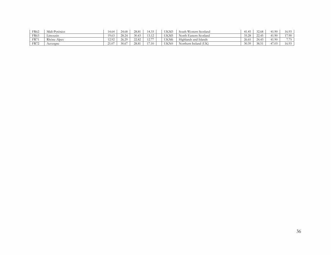
36
FR62 Midi-Pyrénées 14.64 24.68 28.81 14.33 UKM3 South Western Scotland 41.45 32.68 41.90 16.93
FR63 Limousin 19.63 28.24 30.43 13.12 UKM5 North Eastern Scotland 35.28 22.45 41.90 17.90
FR71 Rhône-Alpes 12.92 26.29 22.82 12.77 UKM6 Highlands and Islands 26.65 24.43 41.90 7.75
FR72 Auvergne 21.07 30.67 28.81 17.10 UKN0 Northern Ireland (UK) 30.39 38.51 47.03 16.93

37
Figure A1. Spatial distribution (NUTS 2) of the health dimension in the EU
Note: Thresholds correspond to quintiles; the greener colour, the worst conditions

38
Figure A2. Spatial distribution (NUTS 2) of the knowledge dimension in the EU (the greener, the worst)
Note: Thresholds correspond to quintiles; the greener colour, the worst conditions

39
Figure A3. Spatial distribution (NUTS 2) of the decent standard of living dimension in the EU (the greener, the worst)
Note: Thresholds correspond to quintiles; the greener colour, the worst conditions

40
Figure A4. Spatial distribution (NUTS 2) of the social exclusion dimension in the EU (the greener, the worst)
Note: Thresholds correspond to quintiles; the greener colour, the worst conditions

41
Europe Direct is a service to help you find answers to your questions about the European Union
Freephone number (*): 00 800 6 7 8 9 10 11
(*) Certain mobile telephone operators do not allow access to 00 800 numbers or these calls may be billed.
A great deal of additional information on the European Union is available on the Internet.
It can be accessed through the Europa server http://europa.eu.
How to obtain EU publications
Our publications are available from EU Bookshop (http://bookshop.europa.eu),
where you can place an order with the sales agent of your choice.
The Publications Office has a worldwide network of sales agents.
You can obtain their contact details by sending a fax to (352) 29 29-42758.
European Commission
EUR 26792 EN – Joint Research Centre
Title: Regional Human Poverty Index. Poverty in the regions of the European Union.
Author(s): Dorota Weziak-Bialowolska, Lewis Dijkstra
Luxembourg: Publications Office of the European Union
2014 – 42 pp. – 21.0 x 29.7 cm
EUR – Scientific and Technical Research series – ISSN 1831-9424 (online), ISSN 1018-5593 (print)
ISBN 978-92-79-39642-7 (PDF)
ISBN 978-92-79-39643-4 (print)
doi: 10.2788/10063

42
ISBN 978-92-79-39642-7
doi: 10.2788/10063
JRC Mission
As the Commission’s
in-house science service,
the Joint Research Centre’s
mission is to provide EU
policies with independent,
evidence-based scientific
and technical support
throughout the whole
policy cycle.
Working in close
cooperation with policy
Directorates-General,
the JRC addresses key
societal challenges while
stimulating innovation
through developing
new methods, tools
and standards, and sharing
its know-how with
the Member States,
the scientific community
and international partners.
Serving society Stimulating innovation Supporting legislation
LB
-NA
-26
792
-EN
-N