Poverty Traps and the Social Protection Paradox∗

Munenobu IkegamiInternational Livestock Research Institute

Michael R. CarterUniversity of California, Davis, NBER, BREAD and the Giannini Foundation

Christopher B. BarrettCornell University

Sarah JanzenMontana State University

November 6, 2017

Abstract

Progressively targeted cash transfers remain the dominant policy response to chronic poverty indeveloping countries. But are there alternative social protection policies that might have largerpoverty impacts over time for the same public expenditure? To explore this question, this paperdevelops a dynamic stochastic model of consumption and asset accumulation by householdsthat confront a non-convex production technology and missing financial markets. The modeldemonstrates that a hybrid social protection policy, which devotes resources to funding “stateof the world contingent transfers” (SWCTs) to vulnerable, but non-poor households in thewake of negative shocks, can result in lower rates of poverty in the medium term than doesa conventional cash transfer policy. We also explore the prospects for using subsidized indexinsurance as a way to implement SWCTs and find that an insurance-based hybrid policy canresult in lower total public expenditures than a conventional cash transfer social protectionprogram.

∗Contacts: m.ikegami@cgiar.org; mrcarter@ucdavis.edu; cbb2@cornell.edu; sarah.janzen@montana.edu.An earlier version of this work circulated under the title of “Poverty Traps and Social Protection (Bar-rett et al. (2013)). We thank John Hoddinott, Joe Kaboski, Valerie Kozel, Felix Naschold and seminaraudiences at Cornell, the International Food Policy Research Institute, Namur, Purdue, Wageningen, Wis-consin and the World Bank for helpful comments on earlier versions of this work. Generous financial supportwas provided by the Social Protection Division of the World Bank and by a grant from the USAID Officeof Poverty Reduction to the BASIS Assets and Market Assets Innovation Lab. The ideas expressed are theresponsibility of the authors and should not be attributed to either sponsoring organization.

Poverty Traps and the Social Protection Paradox

Cash transfer programs, progressively targeted at the poorest, have become a predominantpolicy for addressing chronic poverty in developing countries. While pioneered by middleincome developing countries (notably Mexico, South Africa and Brazil), cash transfer pro-grams have spread across the developing world, including the risk-prone pastoral regions ofnorthern Kenya whose economic reality underwrites the analysis in this paper.1 There isample evidence that cash transfers break the liquidity constraints that Loury (1981) arguespropagate poverty inter-generationally by limiting parents’ health and education investmentsin their children. However, there is much more modest evidence that these programs enhancethe earned incomes of recipient households and impact their living standards once the cashtransfers come to an end, despite their theoretical potential to do so.2 Indeed policymakers inLatin America now confront the conundrum of former cash transfer recipients who revert totheir pre-transfer living standards once their transfer eligibility ends. In northern Kenya, theHurrell and Sabates-Wheeler (2013) impact evaluation of the Hunger Safety Net Program(HSNP) cash transfer scheme found that while transfers allowed recipient households to eco-nomically tread water even as their untreated neighbors sunk under the weight of continuingshocks, it did nothing to help recipient households craft a pathway out of poverty. Similar toLatin American countries, Kenya is now looking to augment its HSNP cash transfer programwith a “poverty graduation program.”3

The apparently weak impact of cash transfer programs on the upward mobility of poorhouseholds in at least the medium run has particular salience in risky regions. If cashtransfers do little to promote upward mobility in general, their impact on poverty dynamicsmay be further blunted in risky environments because they do not protect the assets of the

1With the region receiving “emergency” food aid year after year, the Kenyan government in 2009 created asocial protection scheme, the Hunger Safety Nets Program (HSNP), built around bi–monthly cash transferstargeted at the region’s chronically poor and indigent. By regularizing progressively-targeted assistance,HSNP had hoped to put households on a pathway out of poverty by enabling asset accumulation andsustained investment in child health and education so as to avert future chronic poverty arising due toeconomic disability (see the discussion in Hurrell and Sabates-Wheeler (2013)).

2The Gertler et al. (2012) study of Mexico’s Progresa program finds notable investment and incomeeffects from a purely cash transfer program. The Bastagli et al. (2016) review study finds more modestevidence of such effects, unless specific efforts were made by implementers to support planning, investment,and business development. In a similar spirit, the six country studies contained Maldonado et al. (2016)find some evidence that the potential impacts of cash transfers on earned income are when cash transfersare paired with ancillary business development programs targeted at cash transfer recipients.

3The current generation of graduation programs take their inspiration from BRAC’s ultra-poor programthat recognizes that more than liquidity increments may be needed to reduce chronic poverty. Such programsinvolve a mix of cash transfers, financial education, confidence building and coaching, and culminate with anasset transfer. Banerjee et al. (2015) summarize evaluations of graduation programs that span both middleand low income countries.

1

non-poor who are vulnerable to falling into poverty. This omission has two potential effects.First, conventional cash transfers do not stem the downflow of the vulnerable non-poor intopoverty that is driven by shocks (Krishna (2006)). Second, by not protecting the assets of thepoor and the vulnerable non-poor, cash transfers in turn do little to enhance the investmentincentives of the already poor.4 Given these two effects, the population of future poor maygrow, raising the cost of any anti-poverty program.

These observations raise the question whether an alternative social protection schemecan more effectively reduce the extent and depth of poverty when compared to the purelyprogressive targeting rules of standard cash transfer programs. Using a dynamic stochasticprogramming model meant to capture key features of a risky rural landscape like that ofnorthern Kenya, this paper explores the poverty reduction potential of a hybrid social pro-tection system that combines conventional cash transfers targeted at the poorest with stateof the world contingent cash transfers (SWCTs) targeted at the vulnerable, non-poor in thewake of negative shocks.

Our findings include what we call the paradox of social protection. Under the assump-tion that transfers are unanticipated (i.e., that households do not alter their accumulationstrategies in anticipation of social protection benefits), we show that when compared to astandard, progressively targeted scheme, a hybrid policy that diverts some the social protec-tion budget to the vulnerable non-poor results in lower levels of poverty in the medium-term,although poverty rates are higher in the short-term. Conventional cash transfer programsthus implicitly make an intertemporal tradeoff between the well-being of the poor todayversus their well-being in the future. The hybrid program creates the mirror intertemporaltradeoff.

We then relax the assumption that transfers are unanticipated and explore the impactsof hybrid social protection when the contingent transfers are anticipated. We show first thatanticipation crowds in additional accumulation by the poor, who are incentivized by thefact that SWCTs will protect their assets should they invest and advance to the ranks ofthe vulnerable non-poor. This ex ante accumulation effect might be termed positive moralhazard as it induces investment and risk taking by the poor that lessens the overall rateof poverty. At the same time, when SWCTs are precisely targeted at the vulnerable as inour model, a new equilibrium appears. Specifically, a subset of agents accumulate only tothe point where they are eligible for SWCTs, but not beyond. This new equilibrium reflectsa more conventional negative moral hazard, as those at this equilibrium make choices thatincrease the probability of receiving the insurance-like contingent social protection payments.

4Indeed, if anything, it might be expected that means-tested cash transfers would discourage accumulationas successful accumulation could lead to loss of benefits.

2

Given the tradeoffs, expense, and complexities associated with SWCTs and hybrid socialprotection, we then ask whether the impacts of an SWCT can be achieved with an insurancecontract which is co-funded by the government and by the vulnerable non-poor. Rather thanholding the social protection budget fixed, we instead ask how much budget is needed overtime to fully close the poverty gap for all poor households and to pay for the governmentinsurance subsidy that is offered to all poor and vulnerable non-poor households under thehybrid scheme. Drawing on companion work that models the dynamically optimal demandfor insurance (Janzen et al. (2016)), we show that the present value of the required govern-ment expenditure stream is lower under the hybrid insurance scheme than it would be undera conventional cash transfer scheme targeted only at the poor. This cost saving is realizedwithout any tradeoff between the well-being of the poor in the present and the future.

The remainder of the paper proceeds as follows. Section 1 presents a dynamic stochasticmodel of household consumption and asset accumulation in which households enjoy hetero-geneous endowments of assets and productive skill. Section 2 then uses this model to analyzea stylized model of a village economy comprised of 300 households distributed randomly overthe ability-initial asset space that defines the intertemporal choice model. As a baseline forlater analysis of alternative policy regimes, we use dynamic programming methods to simu-late the stylized economy over a sixty year time horizon, tracking the evolution of growth,poverty and a new measure of “unnecessary deprivation.”

Section 3 then explores the impact of alternative social protection schemes, one thattargets transfers in a purely progressive fashion, and another in which the available budgetis targeted according to a triage protocol that prioritizes transfers to households that arevulnerable to slipping into chronic poverty over transfers to already poor households. In thissection, we assume that households do not anticipate transfers. It is here where the paradoxof social protection emerges. By preventing collapse into poverty by agents vulnerable toasset shocks, the triage scheme ultimately reduces the extent of poverty and leads to greatertransfers to and higher welfare for poor households in later years.

Section 4 then relaxes the assumption that transfers are unanticipated and explores whathappens when agents fully anticipate contingent transfers provided to the vulnerable underthe triage scheme. We show that anticipation of these transfers has both positive andnegative effects. Finally we show that implementing the contingent transfers as a partiallysubsidized insurance contract (with co-pays required of beneficiaries) eliminates the negativewhile preserving the positive effects of contingent protection. Section 5 concludes.

3

1 Assets, Ability, Risk and the Multiple Dimensions of

Chronic Poverty

Azariadis and Stachurski (2005) define a poverty trap as a “self-reinforcing mechanism whichcauses poverty to persist.” A robust theoretical literature has identified a variety of suchmechanisms that may operate at either the macro level–meaning that an entire countryor region is trapped in poverty–or at the micro level–meaning that a subset of individualsbecome trapped in chronic poverty even as others escape (Barrett and Carter, 2013, Kraayand McKenzie, 2014, Ghatak, 2015 and Barrett et al. (2016) provide recent review papers).In this paper, we explore the implications of a micro poverty trap mechanism for the designof social protection programs, employing a variant of what Barrett and Carter (2013) callthe “multiple financial market failure” poverty trap model. This model can generate multipleequilibria in the sense that a given individual may end up at the high or the low equilibriumdepending on initial conditions and stochastic realizations.

The semi-arid pastoral region of Northern Kenya, which motivates this work, is an area ofwidespread chronic poverty. Multiple studies, using different data sets, have found evidenceof bifurcated asset dynamics in this region, with households above a critical level tending toa high equilibrium and those below it tending to a low level (Barrett et al. (2006); Lybbertet al. (2004); McPeak and Barrett (2001); Santos and Barrett (2011, 2018)).5 To explore howsocial protection might work in this environment, we build on the Buera (2009) non-stochasticmodel of asset accumulation with two production technologies under credit constraints andheterogeneous agent ability.6 We extend the Buera model by adding asset shocks to allowfor the importance of both ex ante awareness of risk and the ex post experience of shocks askey determinants of poverty dynamics (Elbers et al. (2007)).

We show that multiple poverty trap mechanisms emerge in this setting. Low abilityhouseholds are innately poor, as they never find the high-return technology attractive andthus they endure low incomes indefinitely. Meanwhile, intermediate ability households candramatically change their asset accumulation choices in response to ex ante asset risk and

5Note, these findings do not generalize globally. Broad-based empirical evidence of poverty traps has beenmixed (Subramanian and Deaton, 1996; Kraay and McKenzie, 2014), although Kraay and McKenzie (2014)conclude that the evidence for the existence of structural poverty traps is strongest in rural remote regionslike the arid and semi-arid lands of East Africa. As Barrett and Carter (2013) note, there is a tendency tosometimes conflate the failure to find a multiple equilibrium poverty trap with the non-existence of povertytraps. Poverty traps can of course be single equilibrium, as in Nashold (2013). For a particularly interestinganalysis of the emergence of a multiple equilibrium from a single equilibrium structure, see Kwak and Smith(2013).

6Related previous papers include Becker and Tomes (1979), Loury (1981), Banerjee and Newman (1991),Banerjee and Newman (1993), Galor and Zeira (1993), Ray and Streufert (1993), Aghion and Bolton (1997),Piketty (1997), Carter and Zimmerman (2000), and Ghatak and Jiang (2002).

4

ex post realization of asset shocks. This cohort faces a multiple equilibrium poverty trap ofthe sort on which the literature has long focused. Finally, there is a high ability group thatmay start off poor but will inevitably take up the high-return technology and graduate outof poverty and remain non-poor (in expectation) in the long run.

1.1 A Model of Asset Dynamics and Heterogeneous Ability

Consider an economy in which each individual j is endowed with a level of innate ability (αj)as well as an initial stock of capital (kj0). Preferences are unrelated to the individual’s innateability. In what follows, we treat αj as fixed. We conceptualize the agents in this economyas adults and αj as capturing the predetermined physical stature, cognitive development,and educational attainment with which they entered adulthood and the economy. Thisapproach obviously ignores the origins and evolution of such innate ability. Carter andJanzen (2018) generalize the specification here and allow each dynasty’s human capital toevolve intergenerationally over time through a stochastic process in which ability regressesto the mean level unless compromised by nutritional shortfalls. In this paper, however, weset aside this additional complexity in order to concentrate on exploring social protectionpolicy design in the presence of poverty traps.

Each period the individual has to choose between two alternative technologies for generat-ing income. Both technologies are capital using and skill-sensitive (i.e., for both technologies,more able people can produce more than less able people). One technology (the “high” tech-nology) is subject to a fixed cost, E, such that the technology is not worth using at lowamounts of capital. Specifically, we assume that income, f , for individual j in period t isgiven by

f(αj, kjt) = αj max[fH(kjt), fL(kjt)]

where fL(kjt) = kγLjt , fH(kjt) = kγHjt − Eαj, E > 0 and 0 < γL < γH < 1.7 We denote as

k(α) as the value of capital where it becomes worthwhile to switch to the more productivetechnology (i.e., k(αj) = k|αjfL(k) = αjfH(k)).8

If an individual had access to only one technology, she or he would accumulate capitalup to a unique steady state values k∗L(αj) for the low technology or k∗H(αj) for the hightechnology. The key question is then what happens when the individual has access to both

7Note that fixed costs do not vary by ability level as the division of E by αj is canceled out by thepre-multiplication of the production function by αj , which allows us to more generally keep the notationsimpler.

8By construction, this formulation favors adoption of the high technology by assuming away informationproblems and all other obstacles to adoption other than financing. This simplification eliminates inessentialfactors that would reinforce the effect that are generated here under full information.

5

technologies. In the spirit of Skiba (1978), we ask whether an individual, whose initial capitalstock is below k(αj), will gravitate toward the high or the low technology.9

Consider the case of an individual who begins life with k∗L(αj) < kj0 < k(αj). Notethat because this individual is beyond the low level steady state, but short of the technologyswitch point, incremental returns to further investment are low relative to the cost of foregoneconsumption, discouraging further accumulation. Borrowing constraints, and limited income,make it impossible for the individual to discretely jump over the region of low returns. Willthis individual optimally accumulate assets over time and end up at k∗H(αj) and a non-poorstandard of living? Alternatively, will the individual settle into a poor standard of livingwith capital stock k∗L(αj)? More formally, is there an initial asset threshold, k(αj) < k(αj),

below which individuals slip to the low equilibrium (remaining chronically poor), and abovewhich she or he will move to the high equilibrium (eventually becoming non-poor)?

We analyze this question with a dynamic model of consumption and investment choice.We rule out borrowing and hence consumption every period can be no more than availablewealth, or what Deaton (1991) calls cash on hand:

cjt ≤ kjt + f(αj, kjt),

The household’s stock of accumulated capital evolves over time according to the followingrule:

kjt+1 = (kjt + f(αj, kjt)− ct) (θt+1 − δ) .

where δ is the natural asset depreciation rate and θt ≤ 1 is a random asset shock realizedat the beginning of every period t. Note that θ = 1 implies optimal conditions, whereasθ < 1 indicates less favorable conditions or an unfavorable shock that destroys some fractionof wealth. We assume that (θt − δ) > 0. While in principal θ > 1 might be allowed, suchevents seem unlikely and we will restrict the analysis to the case where only negative shocksare possible.10 The cumulative density function of θt is denoted by Ω(·) and we assume thatevery household knows Ω(·).

In period t households choose their production technology, consumption, and (implicitly)investment based on state variable kjt (asset holdings), αj (innate ability) and the probabilitydistribution of future asset losses (Ω). Households then observe asset shocks θt+1 which

9As first explored by Skiba (1978), with a non-convex production technology, a bifurcated accumulationstrategy could occur around a critical minimum asset level.

10While this assumption mechanically implies lower expected returns relative to the case where someshocks are greater than one (holding f fixed), this assumption does not necessarily imply that returns arelow. Instead, in the spirit of frontier production analysis, k + f(α, k) can be thought of as the maximumachievable cash on hand assuming good conditions, and less than optimal conditions simply means thatreturns are some fraction less than what is maximally obtainable.

6

determine asset losses. The primary timing assumption is that the shocks happen after thehousehold’s decision to save or consume, and then once again all the information needed tomake the next period’s optimal decision is contained in kjt. Assembling these pieces, we canwrite the decision-maker’s intertemporal choice problem as:

maxcjt

Eθ

∞∑t=0

βtu(cjt)

subject to:

cjt ≤ kjt + f(kjt)

f(αj, kjt) = αj max[fH(kjt), fL(kjt)]

kjt+1 = (kjt + f(kjt)− cjt) (θjt+1 − δ)

kjt ≥ 0

(1)

where Eθ is expectation taken over the distribution of the random shock θ, β is the timediscount factor, and u(·) is the utility function defined over consumption cjt and has the usualproperties. Denote the investment rule in the presence of asset shocks as i∗(kjt|αj,Ω).11

1.2 The Micawber Frontier and the Two Dimensions of Chronic

Poverty

As in Skiba (1978) and Buera (2009), this model identifies a critical asset level, denoted k(αj),

around which dynamic behavior bifurcates. An individual with ability level αj will attemptto accumulate the assets needed to reach the high technology equilibrium if she enjoyscapital stock kjτ > k(αj). Otherwise, she will only pursue the low technology, accumulatingthe modest stock of capital that it requires. Note that this frontier, a generalization ofwhat Zimmerman and Carter (2003) call the Micawber Threshold, divides those who havethe wealth needed to accumulate from those who do not.12 We label k(αj) the MicawberFrontier.

The two graphs in Figure 1, created through numerical analysis of the dynamic pro-11More precisely, i∗(kt|α,Ω) is the policy function of the following Bellman equation:

V (kt) ≡ maxitu(f(α, kt)− it) + βE [V (kt+1|kt, it)]

where E [V (kt+1|kt, it)] =

∫V (θt[it + (1− δ)kt])dΩ(θt)

12Skiba (1978) less poetically calls the equivalent threshold in his model a critical cutoff point.

7

Figure 1: The Micawber Frontier and Chronic Poverty

(a) Probability of Chronic Poverty (%)

0

20

40

60

80

100

1.00 1.05 1.10 1.150

2

4

6

8

10

αL αH

Intrinsic Ability, αj

Initi

al C

apita

l, k j1

(b) Risk and the Micawber Frontier

1.00 1.05 1.10 1.15

02

46

810

αL αH

Intrinsic Ability, αj

Initi

al C

apita

l, k j1 k~(α)

kp(α)

k(α)

Micawber Frontier (no risk)Micawber Frontier(risk)Technology Adoption FrontierAsset Poverty Line

1.00 1.05 1.10 1.15

02

46

810

1.00 1.05 1.10 1.15

02

46

810

1.00 1.05 1.10 1.15

02

46

810

gramming model 1, present the Micawber Frontier under the parameterization reported inAppendix 1 that we use to implement the model in the remainder of this paper.13 Alongthe horizontal axes are innate ability or skill levels, ranging left-to-right from least to mostable. The vertical axes measures the stock of productive assets. Figure 1a graphs the prob-ability that a household occupying each initial endowment position will end up chronicallypoor, i.e., at the low level equilibrium. Notice that households on the west/southwest side ofthe figure approach the low level equilibrium with probability one, indicating that for theseendowment positions it is not worthwhile to even attempt the accumulation of the assetsrequired to reach the high equilibrium. As shown in Figure 1b, we define the MicawberFrontier as the locus of skill and assets where the household, behaving optimally accordingto Model 1, switches to a strictly positive probability of escaping chronic poverty. The solidcurve in Figure 1b graphs this locus. Comparing across the two graphs in Figure 1, we cansee that for endowment positions far enough east and north of the Frontier, the probabilityof escaping chronic poverty is one. For middle ability households in the multi-toned bandjust north and east of the Micawber Frontier, the probabilities of escape are modest.

To ease discussion and link it to more conventional poverty analysis, Figure 1 also includesan “asset poverty line,” the dashed downward sloping line, denoted kp(αj). For each abilitylevel, this asset poverty line indicates the stock of assets the individual must have in orderto produce a living standard exactly equal to a money metric poverty line, yp. We defineyp as the level of income that a reference middle ability person (αm = 1.07 in the numericalanalysis) would produce were she in steady state equilibrium at the low technology (yp =

13Buera (2009) provides a formal proof for his non-stochastic model.

8

f(αm, k∗L(αm)). This assumption is of course arbitrary, but it has the rhetorical advantage of

allowing us to label most individuals poor unless they craft a pathway to the high technology.This is desirable in our stylized model as it creates a strong linkage between improvedtechnology adoption, income and poverty measures.

Note that the Micawber Frontier has a behavioral foundation and thus differs from theasset poverty line, which is based on a standard (and therefore arbitrary) income povertyline.14 Those agents whose initial ability-asset endowments place them above the MicawberFrontier but beneath the asset poverty line will be initially poor. With the positive prob-abilities illustrated in Figure 1a, these individuals will prove to only be transitorily pooras they attempt to accumulate their way out of poverty. By contrast, those whose initialendowments situates them beneath the Micawber Frontier but above the asset poverty linewill not be poor initially, but will steadily eat into their asset holdings and will eventuallybecome poor. These movements represent structural transitions across the poverty line.

There can also be stochastic movements around the asset poverty line among the sub-population that finds itself above the Micawber Frontier. For those individuals, small assetshocks may temporarily leave them beneath the asset poverty line without driving themoff their growth path toward the high equilibrium. Such individuals would be seen to be“churning,” to use the language employed by some poverty analysts. Individuals could findthemselves above both the Micawber Frontier and the asset poverty line, in which case theywould be always non-poor assuming they escaped further shocks. Symmetrically, individualsinitially below both the Micawber Frontier and the asset poverty line would always registeras being poor. This simple depiction of the Micawber Frontier and the asset poverty linecaptures the full range of conventional static and dynamic poverty measures.15

As illustrated in Figure 1, the numerical analysis identifies three distinct regions in thespace of ability and initial asset holdings. Irrespective of their capital endowment, high skillindividuals with αj > αH will always move toward the high equilibrium as k(αj) = 0∀ αj >αH . When they reach the technology shift asset threshold k(αj) they will optimally switch tothe higher technology. Irrespective of their starting position, these upwardly mobile agentssteadily converge to the steady state asset value for the high technology. They may be poorover some extended period as they move toward their steady state value, but eventually theyshould become non-poor by virtue of the optimal accumulation behavior induced by theirhigh ability endowment. Such individuals do not face a poverty trap.

In contrast, those with an innate ability level below the critical level αL will never move14As discussed by Carter and Ikegami (2009), this characteristic of the Micawber Frontier makes it an

interesting candidate as the base for chronic poverty measures.15See Carter and Barrett (2006) for a discussion of distinct generations of poverty analysis that encompass

these different ideas.

9

toward the high technology irrespective of their initial asset endowment. This critical skilllevel defines a region of intrinsic chronic poverty, made up of individuals who lack the abil-ity to achieve a non-poor standard of living in their existing economic context.16 Theseindividuals face a single equilibrium poverty trap.

Those in the intermediate skill group with αL < αj < αH have positive but finite valuesk(αj). If sufficiently well-endowed with assets (kj0 > k(α)), these intermediate ability indi-viduals will attempt to accumulate additional assets over time, and will with some strictlypositive probability adopt the high technology and eventually reach a non-poor standardof living. However, if these same intermediate skill individuals begin with assets belowk(αj)—or if a shock pushes them below that level—they will no longer find the high equi-librium attainable and will settle into a low standard of living. Like those in the region ofintrinsic chronic poverty, intermediate ability individuals initially endowed with less thank(αj) will be chronically poor. Unlike the intrinsically chronically poor, the chronic povertyof the intermediate skilled individuals represents needless or unnecessary deprivation in thesense that they could be helped to lift themselves out of poverty with appropriate socialprotection policies, as we discuss below. For a given set of production possibilities, the totalnumber of chronically poor in any society will thus depend on the distribution of householdsacross the ability-wealth space.

Finally note that while some authors (e.g., Barrett and Carter (2013) and Kraay andMcKenzie (2014)) often distinguish between single equilibrium poverty trap models, multipleequilibrium poverty trap models and models without poverty traps, our model shows that allthree possibilities can coexist in a single economy with heterogeneously endowed agents.17

1.3 The Ex-post and Ex-ante Effects of Asset Shocks

The Micawber Frontier is a function of the economic environment in which individuals findthemselves. In particular, the distribution of the stochastic term θ fundamentally shapesinvestment behavior. We now explore the impact of ex ante risk and ex post shocks oninvestment and the long-term evolution of poverty.

The ex post effect of realized shocks comes about simply because negative events maydestroy assets, knocking people off their expected path of accumulation. For upwardly mobileindividuals, such shocks may delay their arrival at the upper level equilibrium, necessitating aperiod of additional savings and asset reaccumulation. But it does not set them on a different

16CPRC (2004) and CPRC (2008) give examples of individuals who suffer such fundamental disabilities.17The econometrics of empirically testing for the existence of poverty traps in the face of this kind of

complexity is not fully developed, although Santos and Barrett (2018) make some important progress in thisregard.

10

accumulation path. Similarly, realized shocks have no long-term effect on the equilibriumtoward which the low ability, intrinsically chronically poor gravitate.

In contrast, the ex post consequences of shocks can be rather more severe for householdsof intermediate ability. Consider the case of a household that is initially slightly above theMicawber Frontier. A shock that knocks it below the frontier will banish the household intothe ranks of the chronically poor as in the wake of the shock, the household will alter itsstrategy and move toward the low equilibrium (divesting itself of assets).

While these ex post effects of shocks are important, the anticipation that they mighttake place would be expected to generate a “sense of insecurity, of potential harm peoplemust feel wary of—something bad can happen and spell ruin,” as Calvo and Dercon (2009)put it. Numerical analysis of the model shows that this sense of impending ruin indeeddiscourages forward-looking households from making the sacrifices necessary to reach thehigh equilibrium. The Micawber Frontier shifts to the southwest once asset risk is removed,as shown in Figure 1b. The dashed curve is the Micawber Frontier in the absence of risk. Theboundaries marking the critical skill levels at which households move between the differentaccumulation regimes also shift out, meaning more intrinsically upwardly mobile householdsand fewer intrinsically chronically poor households when we eliminate the ex ante effects ofrisk.

The most dramatic effects of risk are seen by considering a household whose skill andcapital endowments place it between the two frontiers. Consider a household whose skilland initial asset endowments are represented by the solid circle in the middle of Figure 1b.Absent the risk of asset shocks, such a household would strive for the upper equilibriumand eventually escape poverty. In the presence of risk, such a household would abandon thisaccumulation strategy as futile and settle into a low level, chronically poor standard of living.In the face of asset risk, the extraordinary sacrifice of consumption18 required to try to reachthe high equilibrium is no longer worthwhile, and the household will optimally pursue thelow level, poverty trap equilibrium. By contrast, the shift has no significant behavioral effecton either intrinsically chronically poor households (represented by the solid diamond on theleft side of Figure 1) or intrinsically upwardly mobile households (the solid triangle on theright side of Figure 1).

To explore the differential effects of risk and shocks on these different sub-populations,Carter and Ikegami (2009) use the dynamic choice model above and simulate the incomestreams it generates in three distinct settings:

• A non-stochastic economy in which agents repeatedly apply the optimal investment18The consumption sacrifice is extraordinary because the immediate returns from incremental accumulation

do not outweigh the cost of foregone consumption.

11

rule, i∗n(kjt|αj)19,

• An economy characterized by risk without realized shocks in which agents follow therisk-adjusted optimal accumulation rule, i∗(kjt|αj,Ω), but never actually experienceshocks (a scenario that allows us to isolate the ex ante effects of risk); and,

• A fully stochastic economy, meaning that individuals not only follow the risk-adjustedoptimal investment rule but each period they are subject to a random asset shockgenerated in accordance with the probability structure Ω.

Their simulations show that for the intrinsically chronically poor (low αj) and the upwardlymobile (high αj) groups, the impact of risk and shocks on the realized stream of utilityis relatively modest and attributable almost entirely to the disruptive, ex post effects ofasset shocks. In contrast, for the intermediate ability group, the ex ante behavioral (i.e.,investment disincentive) effects of uninsured risk account for most of the welfare effects ofrisk and shocks. These effects are also large in magnitude for the intermediate ability group.While the discounted income streams for the other two groups fall only 5-10 percent in thefully stochastic scenario, the drop is approximately 25 percent for the intermediate abilitygroup, with roughly 90 percent of the losses due to the ex ante risk effect exclusively.20 Thedifference arises because while risk slightly reduces the desired steady state capital stock forlow and high ability agents, mainly it forces them to occasionally rebuild assets in orderto reattain the desired steady state capital stock. In sharp contrast, intermediate abilityagents may fundamentally shift their investment strategy in the presence of risk, eschewingany attempt at trying to reach the high-level equilibrium open to them, creating addedavoidable chronic poverty.

Among other things, these simulations show that in the presence of critical asset thresh-olds, risk takes on particular importance for those individuals subject to multiple equilibria.Conversely, removal of risk (through social protection or insurance schemes) could in princi-ple generate large benefits for intermediate ability individuals, as we now explore.

19The subscript n denotes this non-stochastic world and i∗n(kt|α) is policy function of the following Bellmanequation:

Vnr(kt) ≡ maxitu(f(α, kt)− it) + βVnr(kt+1|kt, it)

= maxitu(f(α, kt)− it) + βVnr(it + (1− δ)kt)

20Details on these simulation results are available from the authors by request.

12

2 Poverty Dynamics Absent Social Protection

The analysis in the prior section showed that both the anticipation and experience of eco-nomic shocks have a fundamental effect on behavior and welfare in the presence of povertytraps, expanding the portion of the endowment space from which people do not escapepoverty through their own efforts. This observation suggests that social protection policieshave a fundamental role to play in stimulating poverty reduction and economic growth. Buthow will different should social protection policies work in a world with multiple sources ofpoverty traps? As a first step towards answering this question, this section uses the model ofindividual decisionmaking developed above as the basis for analyzing accumulation, growthand poverty in a stylized economy lacking any social protection policies. Sections 3 and 4will then take a careful look at the impact of alternative social protection schemes on thiseconomy.

2.1 The Stylized Economy and Measures of Performance

Consider now an economy comprised of agents whose livelihood choices are described bythe inter-temporal maximization problem 1. To keep things simple, we will assume that allshocks are idiosyncratic and that prices in the economy are unaffected by shocks and byindividuals’ decisions. While these assumptions are clearly at odds with the real world, theypermit us in the first instance to clarify basic principles and tradeoffs in the design of socialprotection policies.21

For purposes of the numerical analysis, we assume that there are 300 agents, each de-scribed by a skill and initial capital stock pair. We allocated agents along the skill continuum,with 25% each in the intrinsically chronically poor and upwardly mobile ranges, and halfthe agents in the intermediate ability range where endowments matter to their accumulationand welfare trajectories. Each agent was then assigned a random initial capital stock drawnfrom a uniform distribution over the zero to ten range. While in any existing economy wewould expect there to be a correlation between skill and observed capital stock, this randomassignment of capital creates an experimental environment in which to study asset dynamicsunder alternative social protection schemes.

The diagram in the northwest corner of Figure 2 shows the initial distribution of abilityand wealth in this stylized economy. Each symbol on the graph represents the initial posi-tion of an individual agent. The solid line is the Micawber Threshold under the stochastic

21When shocks are correlated across households, asset and other prices will begin to covary with householdincome. The implications of this covariance can be important as Carter et al. (2007) discuss empirically inthe case of Ethiopia. Zimmerman and Carter (2003) theoretically examine the implications of such assetprice covariance, showing that it can create another type of poverty trap.

13

environment, while the dashed line is again the asset poverty line. The other graphs in thefigure–to be discussed below–show the evolution of endowment positions under alternativesocial protection policies.

While we can simply focus on the trajectories of agents given their initial endowmentpositions, we also employ a set of summary measures to track the performance of the stylizedeconomy under alternative social protection regimes:22

1. Gross national income (GNI) defined simply as the sum of the incomes of the 300agents. Note that this measure will evolve over time based on capital accumulation (ordeaccumulation) as well as the shift of households between the low and high technologyregimes.

2. Standard static poverty measures based on the Foster-Greer-Thorbecke (FGT) familyof measures:

P yγ =

1

n

∑yj<yp

(yp − yjyp

)γ(2)

where n is the total number of individuals, yp is the income poverty line, yj is individualj’s income, and γ is the usual FGT sensitivity parameter. We will specifically focuson the popular headcount (P y

0 ) and poverty gap (P y1 ) measures. As discussed above,

we set the poverty line yp at the level of income that a medium skill individual wouldproduce in steady state if she had access only to the low technology.

3. A novel measure of unnecessary deprivation, Dyγ. This measure resembles the FGT

poverty gap measure, in that it focusses only on those beneath the income povertyline. In addition, Dy

γ focuses only on the subset of the poor who have the skill orhuman capability to reach the high equilibrium, αj > αL. Denoting the maximumsteady state income available to individuals with αj > αL as yj∗ = αjfH(k∗H(αj)), wedefine the unnecessary deprivation gap as yj∗−yj, we define our measure of unnecessarydeprivation as:

Dyγ =

1

n

∑yj<ypαj>α

L

(yj∗ − yjyj∗

)γ. (3)

As with the FGT measure, γ is a sensitivity parameter, with γ = 0 offering a head-count of unnecessary deprivation, γ = 1 measuring the money metric unnecessarydeprivation gap, and γ > 1 placing greater weight on larger underperformance relative

22In work not reported here, we also analyzed the impacts of the different policies using a conventionalBenthamite social welfare function as well as the dynamic poverty measures suggested by Calvo and Dercon(2007). The qualitative story told by these measures is similar to that which can be gleaned from themeasures discussed here.

14

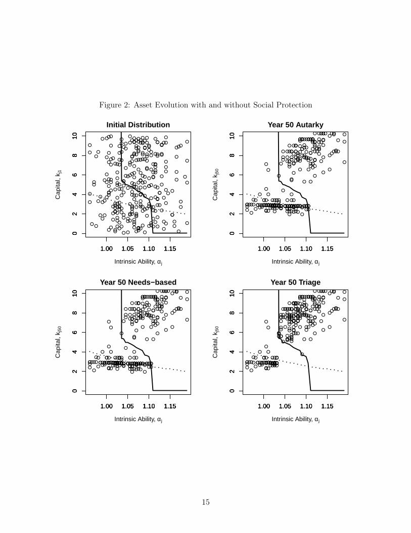
Figure 2: Asset Evolution with and without Social Protection

1.00 1.05 1.10 1.15

02

46

810

Initial Distribution

Intrinsic Ability, αj

Cap

ital,

k j1

1.00 1.05 1.10 1.15

02

46

810

1.00 1.05 1.10 1.15

02

46

810

1.00 1.05 1.10 1.15

02

46

810

Year 50 Autarky

Intrinsic Ability, αj

Cap

ital,

k j50

1.00 1.05 1.10 1.15

02

46

810

1.00 1.05 1.10 1.15

02

46

810

1.00 1.05 1.10 1.15

02

46

810

Year 50 Needs−based

Intrinsic Ability, αj

Cap

ital,

k j50

1.00 1.05 1.10 1.15

02

46

810

1.00 1.05 1.10 1.15

02

46

810

1.00 1.05 1.10 1.15

02

46

810

Year 50 Triage

Intrinsic Ability, αj

Cap

ital,

k j50

1.00 1.05 1.10 1.15

02

46

810

1.00 1.05 1.10 1.15

02

46

810

15

to potential. In our subsequent calculations, we rely on the unnecessary deprivationheadcount measure.23

Together, these economic core measures permit us to track over time both the economiccosts (foregone output and unexploited technological opportunities) and the human costs(low standards of living and unnecessary deprivation) of poverty traps.

2.2 Baseline Case of No Social Protection

The northeast panel of Figure 2 shows the asset distribution after 50 years of simulatedhistory for our stylized economy. As can be seen, the asset distribution (which was originallyrandomly distributed independently of the ability distribution) has bifurcated, with a strongpositive correlation between innate ability and wealth. One set of individuals has comfortablysettled above the Micawber Frontier at the high technology steady state. The other groupis at the low level steady state, below the asset poverty line. There are quite a few poorindividuals in the middle ability group whose potential to reach the high equilibrium hasbeen blocked by their low initial asset levels, or realized asset shocks, that trapped thembelow the Micawber Frontier.

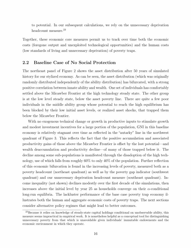
With no exogenous technical change or growth in productive inputs to stimulate growthand modest investment incentives for a large portion of the population, GNI in this baselineeconomy is relatively stagnant over time as reflected in the “autarky” line in the northwestquadrant of Figure 3. This reflects the fact that the positive accumulation and associatedproductivity gains of those above the Micawber Frontier is offset by the lost potential—andwealth deaccumulation and productivity decline—of many of those trapped below it. Thedecline among some sub-populations is manifested through the disadoption of the high tech-nology, use of which falls from roughly 60% to only 40% of the population. Further reflectionof this economic bifurcation is found in the increasing levels of poverty, measured both as apoverty headcount (northeast quadrant) as well as by the poverty gap indicator (southwestquadrant) and our unnecessary deprivation headcount measure (southeast quadrant). In-come inequality (not shown) declines modestly over the first decade of the simulations, thenincreases above the initial level by year 25 as households converge on their α-conditionallong-run equilibria. The lackluster performance of the base case poverty trap economy il-lustrates both the human and aggregate economic costs of poverty traps. The next sectionsconsider alternative policy regimes that might lead to better outcomes.

23Because it relies on knowledge of steady-state capital holdings conditional on unobservable ability, thismeasure seems impractical in empirical work. It is nonetheless helpful as a conceptual tool for distinguishingunnecessary poverty from that which is unavoidable given individuals’ immutable endowments and theeconomic environment in which they operate.

16

Figure 3: Economic Evolution under Alternative Social Protection Policies

0 10 20 30 40 50

450

500

550

600

GNI

year

0 10 20 30 40 50

450

500

550

600

0 10 20 30 40 50

450

500

550

600

0 10 20 30 40 50

0.2

0.3

0.4

0.5

Poverty Headcount

year

0 10 20 30 40 50

0.2

0.3

0.4

0.5

0 10 20 30 40 50

0.2

0.3

0.4

0.5

Autarky Needs−based Triage

0 10 20 30 40 50

0.00

0.02

0.04

0.06

0.08

0.10

Poverty Gap

year

0 10 20 30 40 50

0.00

0.02

0.04

0.06

0.08

0.10

0 10 20 30 40 50

0.00

0.02

0.04

0.06

0.08

0.10

0 10 20 30 40 50

0.1

0.2

0.3

0.4

0.5

0.6

Unnecessary Deprivation Headcount

year

0 10 20 30 40 50

0.1

0.2

0.3

0.4

0.5

0.6

0 10 20 30 40 50

0.1

0.2

0.3

0.4

0.5

0.6

17

3 Poverty Dynamics with Unanticipated Social Protec-

tion

This section examines the impact of reactive food aid or unanticipated social protectionpolicies on the stylized economy studied in the prior section. The label ’unanticipated’signals that these policies are implemented ex post of shocks and we assume away agents’anticipation of the resulting transfers and the behavioral response that would follow fromsuch anticipation. This simplification is made to help understand more clearly how povertydynamics shift in response to different sorts of social protection policies. In particular, weseek to illustrate clearly the value of addressing the purely ex post effects of asset shocks, evenif agents do not expect transfers. Section 4 below will relax the assumption that householdsfail to anticipate and respond to social protection policies.

For all alternatives, we assume that the social protection agency24 has access to an annualbudget that amounts to 2.5% of initial GNI.25 This arbitrary amount was chosen because it isinsufficient to lift all initially poor individuals above the poverty line, though it is enough tosubstantially close the poverty gap. We further assume that the social protection agency hasaccess to full information, including household ability and asset holdings, realized shocks andknowledge of the production technology. While these are implausibly strong assumptions,using them to explore targeting of this limited assistance budget helps further illustrate theworkings of the multiple poverty trap economy.

3.1 Poverty and Aid Traps under Progressive, Means-tested Cash

Transfers

Under the progressively-targeted or needs-based scenario, the agency uses its budget onlyfor progressively targeted, humanitarian/cash transfers. After each production cycle, itcalculates the total poverty shortfall for the economy, S =

∑yj<yp

(yp − yj). If the availablebudget B exceeds the shortfall (B

S> 1), then all poor individuals are given transfers to

increase their income to the level of the poverty line. If BS< 1, then each poor individual

is given transfers that move them to an income level equal to BSyp. Note that this targeting

methods makes the largest transfers to the least well-off but as the ranks of the poor grow,S increases and thus each individual poor person’s transfer receipt shrinks. The transfer

24We use the broad term social protection agency to encompass local or national governments as well asnon-governmental organizations (NGOs) that might respond to shocks.

25We ignore the source of taxation that generates these resources and the associated distortionary effectson the economy. They could be conceptualized as either external resources (brought in by a donor, an NGOor a relief agency), or as domestic tax resources transferred from another sector of the national economy.

18

simply adds an increment to the first (budget) constraint in optimization problem 1. Onceindividuals receive the transfer, they make their consumption versus investment decisionaccording to the same logic of problem 1 above and assume that future transfers will neveroccur. Section 4 relaxes this strong assumption, but for now it helps to understand thedifferent effects of alternative social protection policies.

The impact of this needs-based assistance regime on asset distribution can be seen inthe southwest diagram in Figure 2. The figure is quite similar to that under autarky (thenortheast panel), except that asset levels are somewhat higher for those below the povertyline, especially among lower ability persons, reflecting a transfer rule based on realized in-come levels and the exogenous injection of resources, B, into the economy that manifestas individual transfers to the current poor. Turning to Figure 3, we see that the povertyheadcount and unnecessary deprivation measures follow a trajectory nearly identical to thatwhich emerges absent social protection. While standard cash transfers do not fundamentallyalter poverty dynamics, they do reduce the poverty gap. As can be seen in the southwestgraph of Figure 3, the injection of well-targeted external resources cuts the poverty gaprelative to the no social protection policy regime. But, the steady creation of newly poorhouseholds over time due to adverse asset shocks causes the FGT(1) to steadily rise afteryear 10 of the simulation because the transfer received by any individual poor householdshrinks as more poor people compete for a fixed aid budget, leading to an increasing povertygap. GNI is higher in the economy with needs-based transfer, but this is largely an artifactof the exogenous aid resources that are transferred into the economy via the cash transfermechanism.

In a world where budgets for transfers are available exogenously (e.g., via unrequitedtransfers associated with overseas development assistance), progressively-targeted transfersthat flow to the chronically poor plainly reduces income and asset poverty, if only becausethere are added resources in this scenario. However, these transfers do not fundamentallyalter the economy’s dynamics. Indeed, the troubling irony is that poverty grows in thiseconomy in spite of these transfers as some agents suffer asset shocks that drop them intopoverty but then receive insufficient transfers to enable them to climb back out of povertyon their own. Transfer policies that are designed to respond to one poverty trap mecha-nism–low innate ability that leads to chronically low income–systematically fail to addressthe other poverty trap mechanisms in this economy by failing to prevent more people frominadvertently falling into the trap over time.

These results signal what might be termed a relief trap. By failing to stem the flowof intermediate ability individuals below the Micawber Frontier, the fixed humanitarianassistance budget becomes less and less able to meet the needs of those below the poverty

19

line. If the social protection agency (or the international community) were intent on holdingpoverty at, say, year 10 levels, then increasing fractions of total public expenditures wouldneed to be devoted to aid budgets to accommodate the inflow of the unnecessarily poorwho have suffered severe asset shocks and fallen into the basin of attraction of their low-level equilibrium.26 We abstract here from the standard public finance problems of raisingrevenues, but clearly the growing demands for transfers would have to be met either throughincreasingly distortionary taxation or through reducing funds available for developing newtechnologies, building schools and infrastructure, or other interventions (not modeled here)that are aimed at boosting productivity. Poverty traps can thus, in a very direct way, createrelief traps for purely progressively targeted social protection programs.

3.2 State of the World Contingent Transfers

As the prior simulations make clear, asset risk in our model creates an ever increasingamount of unnecessary deprivation that eventually overwhelms the capacity of needs-basedcash transfers to provide relief, as seen in the rising poverty gap and headcount measures inFigure 2. This observation suggests that a social protection scheme targeted at the vulnerablein the vicinity of the Micawber Frontier-–i.e., a safety net designed to stem the increase inunnecessary poverty—can potentially generate a win-win-win scenario, with higher rates ofimproved technology adoption and GNI growth, reduced poverty (especially for intermediateability groups), and less stress on the social protection budget.

To explore this idea, we initially analyze a harsh “triage” policy regime in which the socialprotection agency provides transfers to households according to the following rules:

1. Each time period, the available budget, B, is allocated with first priority to individualspushed below the Micawber Frontier by negative shocks. Denote these threshold-basedtransfers as SWCTs (State of the World Contingent Cash Transfers). An individual j iseligible for a SWCT of amount SWCTj = k(αj)−θt[ijt+(1−δ)kjt] if ijt+(1−δ)kjt >k(αj) and θjt[ijt + (1 − δ)kjt] < k(αj). In words, if an individual was above theMicawber Frontier prior to the most recent asset shock, but below it afterward, theagency provides a transfer to move the household back to the Micawber Frontier. If the

26There is a complex set of changes occurring in these simulations, which begin from an arbitrary dis-tributions of assets across the ability distribution. The decline (but not the elimination) of unnecessarydeprivation shows that some individuals are adjusting to a new steady state in which they are not poor.Similarly, some low ability individuals who were arbitrarily assigned large initial stocks of assets also dissaveand eventually become poor over time. Finally, some number of households get pushed below the householdswhen large shocks are realized. This latter group is reflected in the slow but steady increase in the povertyand deprivation measures in the out-years of the simulation suggesting that the pressure for an increasingaid budget moderates, but is not completely eliminated over time as households settle into their new steadystates.

20

total budget is no less than the total eligible contingent transfers (B ≥∑J

j=1 SWCT j),then all individuals pushed below the threshold are given an asset transfer to lift themexactly back to it. If the budget is insufficient to cover all SWCTs, then it is allocatedfirst to those closest to the Micawber Frontier so as to minimize the increase in theheadcount of unnecessary deprivation.

2. If there is any remaining budget after step 1 (i.e., if B >∑J

j=1 SWCT j), then thosemid-ability individuals already below the Micawber Frontier (due to low initial inher-itance or prior bad luck not remedied by an SWCT transfer) are given priority forasset transfers that lift them over the Micawber Frontier.27 Analogous to stage 1, totalpotential spending on asset transfers is calculated (denote this total amount as CN).If CN > B −

∑Jj=1 SWCT j, then the budget is again prioritized in order to minimize

unnecessary deprivation , by first helping the most vulnerable, defined as those closestto the Micawber Frontier.

3. If B > SWCT+CN , then the residual budget is allocated according to the progressiveor needs-based formulation discussed in the previous sub-section.

This triage policy would be difficult to implement in most places due to the daunting informa-tion requirements it imposes—knowing the Micawber Frontier, individual ability, individual-specific shocks, etc. We develop this as a thought experiment because it captures clearlythe intertemporal tradeoffs inherent to a system characterized by multiple poverty mecha-nisms. Figures 2 and 3 illustrate the results of this assistance regime for our stylized povertytrap economy. The results stand in strong contrast to autarky and needs-based assistancesimulations. As shown in the southeast panel of Figure 3, by year 50, all most unnecessarydeprivation is eliminated and the headcount of total poverty levels off at 25%, the shareof the population that is intrinsically chronically poor by construction. Compared to thestandard cash transfer policy, technology adoption is higher, as is GNI. In the longer-run,this triage approach to development assistance plainly outperforms needs-based assistanceby any of these metrics.

However, the southwest diagram in Figure 3 illustrates a core ethical challenge associatedwith vulnerability-targeted social protection. The FGT(1) poverty gap measure is lower un-der progressively-targeted cash transfers for the first 8-10 years of the simulation because

27Barrett (2005) refers to this kind of asset transfer as a cargo net transfer as it is intended to lift peopleabove – or help people climb over – thresholds at which accumulation dynamics bifurcate. Note that assettransfers are distinct from SWCT safety net transfers that keep people from beneath those same thresholds.Graduation programs centered on asset transfers to the capable poor, like those described in Banerjee et al.(2015) and Gobin et al. (2017), are the real world analogue to these asset or cargo net transfers.

21

needs-based assistance flows primarily to the least well-off while the stylized vulnerability-targeted policies are aimed at the vulnerable non-poor nearest the Micawber Frontier. But,paradoxically, after 8-10 years, those who are poor are better off under the triage design be-cause it reduces the number of people needing assistance, allowing the fixed social protectionbudget to provide more generous support to those who inevitably need it due to irreversiblylow ability. But, prior to that time, individuals who are poor, and especially the poorest,are better off under needs-based targeting. The results for (asset or income) inequality (notshown) are qualitatively similar, with needs-based transfers generating lower inequality in theeconomy over the first 8-10 years, but threshold-based transfers generating lower inequalityover longer horizons. These results underscore the difficult tradeoffs inherent to the designof social protection policy, both over time and across sub-populations of the poor. In thepresence of multiple poverty trap mechanisms, these tradeoffs become especially sharp.28

4 Moral Hazard and the Design of Anticipated Social

Protection

The analysis in Section 3 revealed the paradoxes and challenges of social protection in aneconomy characterized by poverty traps that take several forms. That analysis, however,unrealistically assumed that individuals do not anticipate social protection benefits. Thislacunae is especially important for state of the world contingent transfers that are targetedat the vulnerable. Such transfers operate as a form of insurance, and as discussed above, thisinsurance might alter ex ante investment incentives for households both above and belowthe Micawber frontier itself.

In this section we therefore relax the assumption that contingent transfers are unan-ticipated and consider households’ rational response to them. While we could in principleanalyze endogenous response to anticipated, progressively-targeted cash transfers, we limitour attention here to anticipated vulnerability-targeted social protection schemes.29

28In additional simulations not reported here, we considered whether these tradeoffs could be mitigatedby mixing different kinds of transfers and/or by reallocating budgets intertemporally through borrowing.While these alternatives can reduce the magnitude of the tradeoffs reported here somewhat, they cannot beeliminated entirely. This underscores the unavoidable nature of the targeting tradeoffs in both cross-section(between different sub-populations of the poor and vulnerable) and over time in a multiple poverty trapeconomy.

29This choice is primarily made for analytical convenience as under the triage policy developed in Section3, the magnitude of cash transfer payments is itself uncertain, depending on the vagaries of the weather thatdictate the residual budget left for such transfers. Clearly, we would expect cash transfers to discourageprivate accumulation (Hubbard et al. (1995) give an empirical example showing how means-tested socialinsurance programs discourage precautionary savings in the United States). By ignoring these disincentiveeffects, we are thus overstating the possible effiectiveness of cash transfers, which only reinforces our broader

22

Figure 4: Nature’s Tax Rates under Contingent Social Protection

(a) Expected Asset Losses (b) Marginal Tax Rates

4.1 Positive and Negative Moral Hazard

We expect two kinds of household response to safety net transfers. First, since safety nettransfers mitigate asset risk, households are willing to accumulate more assets ceteris paribus.This is canonical moral hazard, in that the provision of some insurance induces increasedrisk taking.30 In this model, accumulation of assets subject to stochastic shocks is the onlyrisk-taking behavior available to agents. But asset accumulation is socially desirable inthis setting, as it increases productivity and adoption of improved production technologies,increases GNI and reduces poverty. We therefore call this incentive effect “positive moralhazard.”

Second, because the safety net transfers are conditional (on pre- and post-shock assetholdings) and given the standard intertemporal tradeoff between current consumption andsaving for future consumption, ceteris paribus households have an incentive to satisfy thetransfer condition as often as possible so as to receive extra resources. If some externalagency or government will insure them against falling into a poverty trap, households donot need to self-insure through asset accumulation to the same degree, thereby creating adisincentive to invest beyond the Micawber Frontier that defines eligibility – equivalently,reducing the need for precautionary savings – that runs counter to social objectives. Wetherefore label this effect “negative moral hazard.”

For a middle ability person with k(αj) = 5, Figure 4a shows expected asset losses as afunction of level of capital stock held with (the dashed, red line) and without (the solid,green line) the SWCT policy. As can be seen, there is zero chance of asset losses exactly atthis threshold, and expected asset losses above the threshold will always keep the individual

point.30Recognize that risk is increasing in asset holdings because θ is a multiplicative shock and independent

of k. Therefore, stochastic losses are greater when k is larger.

23

at or above k. When these contingent transfers of the vulnerability targeted social protectionare anticipated, the individual’s optimization problem 1 can be rewritten as follows:

maxcjt

Eθ

∞∑t=0

βtu(cjt)

subject to:

cjt ≤ kjt + f(kjt)

f(αj, kjt) = αj max[fH(kjt), fL(kjt)]

kjt+1 =

k(αj) if

(f(kjt)− cjt) + (1− δ)kt > k(αj) and

(kjt + (f(kjt)− cjt) (θjt+1 − δ) < k(αj)

(kjt + f(kjt)− cjt) (θjt+1 − δ) otherwise

kjt ≥ 0

(4)

This is the same as the problem specified in Section 2 except for the important change inthe law of motion governing kjt+1 now that households are aware of and respond to thecontingent transfers.31

Figure 5 illustrates the impact of the anticipation of contingent transfers on the proba-bility of chronic poverty. For ease of comparison, Figure 5a repeats the probabilities whenthese transfers are not anticipated (from Figure 1a). Comparing Figures 5b and 5a, we seethat substantially fewer endowment positions are likely to end up chronically poor. Thisadditional accumulation induced by the presence of contingent transfers at the (autarky)Micawber Frontier precisely represents positive moral hazard.

While the vulnerability-targeted contingent transfers incentivize upward mobility, theyalso have a discouraging effect on further accumulation that takes households beyond thesafety of k(αj) where assets are fully protected. A large swath of middle ability agents endup in long-term equilibrium at exactly k(αj). This behavior represents classic negative moralhazard as the presence of the implicit insurance provided by the contingent transfer leads

31The household problem at period t can be represented in Bellman Equation form as:

V (kt) ≡ maxitu(f(α, kt)− it) + βE [V (kt+1|kt, it)]

where E [V (kt+1|kt, it)] =

∫V (kt+1(kt, it, θt, kg, δ))dΩ(θt)

kt+1(kt, it, θt, kg, δ) =

kg if it + (1− δ)kt > kg and θt[it + (1− δ)kt] < kg

θt[it + (1− δ)kt] otherwise

24

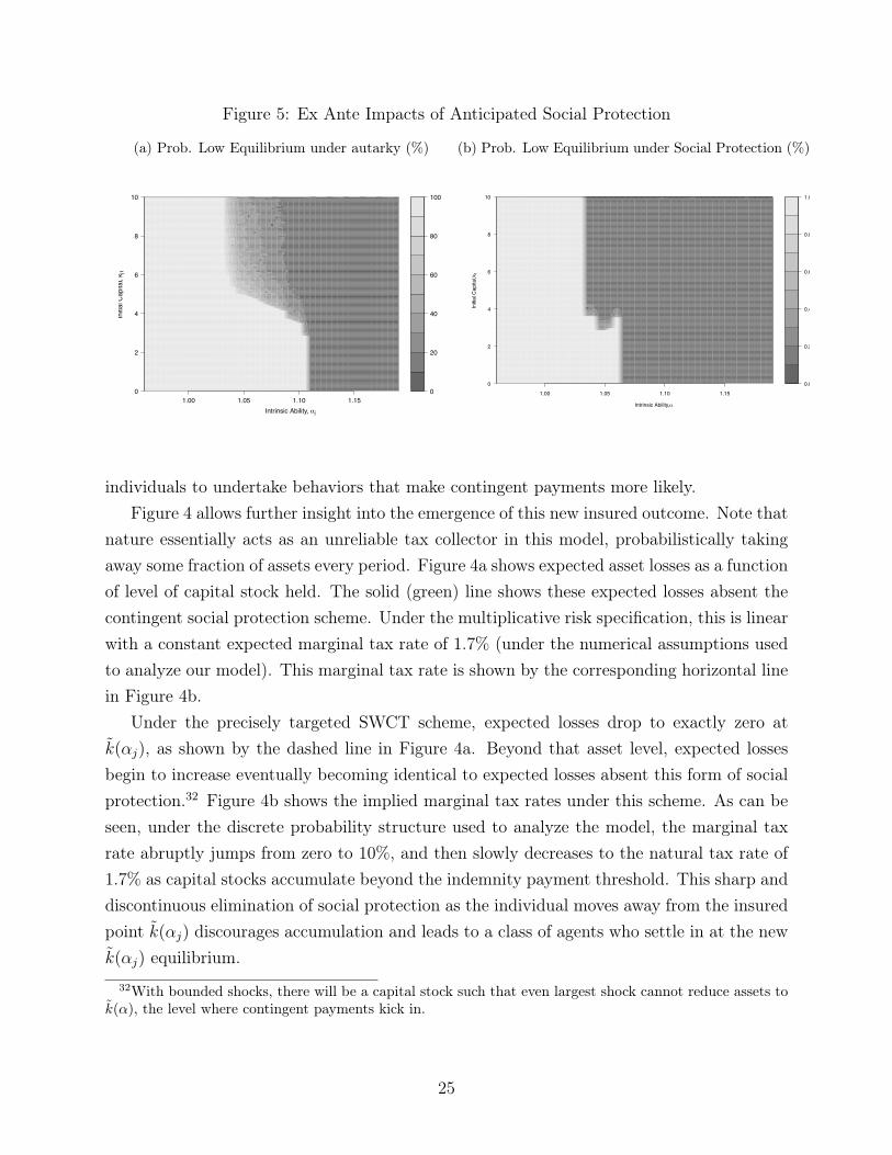
Figure 5: Ex Ante Impacts of Anticipated Social Protection

(a) Prob. Low Equilibrium under autarky (%)

0

20

40

60

80

100

1.00 1.05 1.10 1.150

2

4

6

8

10

Intrinsic Ability, αj

Initi

al C

apita

l, k j1

(b) Prob. Low Equilibrium under Social Protection (%)

0.0

0.2

0.4

0.6

0.8

1.0

1.00 1.05 1.10 1.15

0

2

4

6

8

10

Intrinsic Ability,α

Initi

al C

apita

l,k1

individuals to undertake behaviors that make contingent payments more likely.Figure 4 allows further insight into the emergence of this new insured outcome. Note that

nature essentially acts as an unreliable tax collector in this model, probabilistically takingaway some fraction of assets every period. Figure 4a shows expected asset losses as a functionof level of capital stock held. The solid (green) line shows these expected losses absent thecontingent social protection scheme. Under the multiplicative risk specification, this is linearwith a constant expected marginal tax rate of 1.7% (under the numerical assumptions usedto analyze our model). This marginal tax rate is shown by the corresponding horizontal linein Figure 4b.

Under the precisely targeted SWCT scheme, expected losses drop to exactly zero atk(αj), as shown by the dashed line in Figure 4a. Beyond that asset level, expected lossesbegin to increase eventually becoming identical to expected losses absent this form of socialprotection.32 Figure 4b shows the implied marginal tax rates under this scheme. As can beseen, under the discrete probability structure used to analyze the model, the marginal taxrate abruptly jumps from zero to 10%, and then slowly decreases to the natural tax rate of1.7% as capital stocks accumulate beyond the indemnity payment threshold. This sharp anddiscontinuous elimination of social protection as the individual moves away from the insuredpoint k(αj) discourages accumulation and leads to a class of agents who settle in at the newk(αj) equilibrium.

32With bounded shocks, there will be a capital stock such that even largest shock cannot reduce assets tok(α), the level where contingent payments kick in.

25

4.2 Using Index Insurance and Co-pays to Implement State of the

World Contingent Social Protection

Negative moral hazard and the attraction of k(αj) as a new equilibrium reflect in part theextremely precise targeting of the contingent transfers (and sharp jump in marginal taxrates) that define the vulnerability-targeted social protection scheme. However, this kindof precise targeting is of dubious relevance in the real world where neither realized shocks,asset levels, the Micawber Frontier nor individual skills are easy to observe. Together, theseobservations raise the question as to whether something akin to SWCTs can be implementedusing a market-based microinsurance scheme. Index insurance, which delivers payouts topolicy holders on the basis of a pre-determined index unaffected by the behavior or skill ofthe insured, could be particularly useful. Index insurance offers four potential advantages:

1. Payments can be triggered by a relatively cheap-to-observe index that signals shocks;33

2. It can rely on self-selection through the purchase of insurance, obviating the need toobserve skill;

3. It can require a co-payment, reducing costs, allowing the available public budget tostretch further and enhancing individual investment incentives relative to the SWCTcase; and,

4. If cost reductions are sufficiently strong, reliance on insurance may eliminate the needfor a precisely-targeted subsidy that create the behaviorally perverse sharp discontinu-ities in the effective marginal tax rate, as explored in Section 4.1 above.

Janzen et al. (2016) employ a dynamic model similar to that developed here, while ignoringskill heterogeneity. The analysis compares an autarky scenario in which insurance is unavail-able, and a targeted insurance subsidy scenario in which the government pays half of thecommercial insurance premium (assuming a 20% markup) for all households that hold assetsless than the level required to generate an average income equal to 150% of the poverty line.In all cases, the simulation assumes that households behave optimally based on the price ofinsurance and the dynamic choice problem displayed above.

The Janzen et al. (2016) analysis shows a 50% insurance subsidy (offered across the boardto all but the wealthiest agents) can induce investment and upward mobility (positive moralhazard), but without the negative moral hazard seen in section 4.1 above. Importantly,

33For the specific case of northern Kenya, see the discussion of an index insurance design in Chantaratet al. (2013).

26

Figure 6: Costs of Alternative Social Protection Schemes

they show that under the assumptions of their model,34 the total social protection budget(defined as funds for the insurance subsidy plus funds for cash transfers needed to close thepoverty gap for all poor households) quickly becomes lower under a combined insurance-cashtransfer scheme than under a pure cash transfer scheme. As shown in Figure 6, total costsare in fact higher in the short run under the hybrid scheme, but they become lower as theinduced upward mobility eventually reduces the cost of cash transfers. Under their numericalassumptions, the present value of total social protection expenditures is 16% lower underthe hybrid scheme.

The feasibility of using index insurance to offer contingent protection has been extensivelystudied in the semi-arid regions of northern Kenya. Chantarat et al. (2013) and Mude et al.(2009) describe an initial contract design used in this region, and Jensen et al. (2017) andJanzen and Carter (2016) report empirical impact evaluation results that are consistentwith the expected ex ante and ex post effects of contingent social protection that havebeen explored theoretically in this chapter. Despite these empirical findings, demand for theavailable insurance in Northern Kenya has remained modest. At least partially in response to

34The parameters of the model deviate from those used in the other simulations in this paper. Whilethe results are not directly comparable, the findings are still insightful. Notably, the Janzen et al. (2016)model must assume some level of basis risk (the difference between realized losses and the index). The modelassumes relatively low basis risk. In practice, this is likely to overestimate the benefits of index insurance ifbasis risk is high.

27

this puzzle, the government of Kenya has recently launched multiple programs that offer stateof the world contingent social protection, including distribution of free livestock insurancethrough its KLIP (Kenya Livestock Insurance Program). The government also offers ascalable version of its core social protection scheme (the HSNP program), which extendsbenefits to vulnerable (but not abjectly poor) households when objective indicators signaldrought conditions. The impacts of these new programs, and their ability to fundamentallyalter poverty dynamics as this chapter’s theoretical analysis suggests, remain to be seen.

5 Conclusions

This paper has put forward a dynamic stochastic model of a stylized poverty trap economy inwhich asset risk plays a major role and heterogeneity of individual ability creates two typesof chronic poverty. Some people are chronically poor because their innate ability condemnsthem to a low standard of living. Others suffer unnecessary deprivation simply becausethey inherit insufficient productive capital to reach the critical asset or Micawber frontier atwhich it becomes optimal to make the short-term sacrifices necessary to accumulate assetsand (probabilistically) escape chronic poverty. Each of these two poverty trap mechanismsinvites a different policy response. When both types of chronic poverty co-exist, therefore,tradeoffs inevitably arise in developing cost-effective poverty reduction strategies.

Using this framework, we have shown that purely progressively-targeted social relief—suchas cash transfers—can fall prey to an aid trap because it does nothing to address the rootcauses of poverty. In particular, it does not protect the assets of those of intermediate abilityand wealth who are vulnerable to asset shocks and to becoming poor over time. Membersof this latter group steadily fall into avoidable chronic poverty, adding to the pool of indi-viduals suffering unnecessary deprivation and needing income support. As a result, whilepurely progressively-targeted social protection initially reduces the depth of poverty, the lotof the poor deteriorates over time due to increasing competition for limited social protectionresources. Moreover, an unadorned, purely progressively-targeted system of social protectiondoes not appreciably change the number of poor, nor does it enhance wealth accumulation,economic output or adoption rates of improved technologies.

We have then shown that a hybrid policy, which issues state of the world contingent trans-fers (SWCTs) to vulnerable-but-not-indigent households, eliminates unnecessary deprivation,empowers upward mobility and boosts growth through endogenous asset accumulation andadoption of improved technologies. While this hybrid policy still confronts important trade-offs among different poor people and over time, this theoretical exercise establishes thepotential gains to social protection that targets vulnerability (not just abject poverty) and

28

thereby creates economic multipliers. However, despite these gains, household anticipationof SWCTs discourages some from accumulating assets beyond the range where they remaineligible for social protection transfers.

A key question then becomes whether the balance between positive and negative moralhazard can be altered by changing the mode of delivering contingent transfers. Drawing onthe work of Janzen et al. (2016), we have argued that imprecisely targeted partial subsidiesfor index insurance can achieve the benefits of SWCTs and strike a better balance betweenpositive and negative moral hazard, encouraging upward mobility but not artificially brakingit with means-tested cutoffs. While there are challenges to implementing SWCTs via aninsurance mechanism in practice, a hybrid social protection system that mixes insurancesubsidies and cash transfers in theory appears to be a more cost-effective than standard cashtransfers as a way to address chronic poverty in risk-prone regions like Northern Kenya.

Ultimately, the key finding of this paper is that poverty traps characterized by multipleequilibria can have a pronounced effect on the performance and design of policies intended tostimulate poverty reduction, economic growth and uptake of improved production technolo-gies. There are potentially large returns to developing and using knowledge about criticalasset thresholds to target assistance to the vulnerable non-poor. The co-existence of popula-tions facing different sorts of poverty traps, however, also raises unavoidable, thorny tradeoffsamong distinct cohorts of the poor, as well as difficult intertemporal tradeoffs between cur-rent and future poverty reduction.

29

Appendix 1: Parameters and Other Details for Numerical

Simulation

This section provides additional detail on the formal model used to generate the resultsdiscussed in the main body of the paper.

The functional specification for the utility function u(·) is

u(ct) =c1−σt − 1

1− σ

The probability density of θt is assumed to be:

density of θt =

0.90 if θt = 1.0

0.05 if θt = 0.9

0.03 if θt = 0.8

0.02 if θt = 0.7

The other structural parameter values are assumed as follows: σ = 1.5, δ = 0.08, β = 0.95,γL = 0.3, γH = 0.45, E = 0.45.

We discretize continuous variables k and α as follows: k = 0.05, 0.10, . . . , 15.00 andα = 0.960, 0.965, . . . , 1.190.

For the simulation of the stylized economy of 300 individuals we draw α from N(1.070, 0.0552),with the mean and variance chosen so that ex ante proportion of low, middle, and high typeindividuals (defined relative to the stochastic Micawber Frontier) would be 25%, 50%, and25%, respectively. We draw k1 from Uniform[0.1, 10.0] and assume that k1 and α are statis-tically independent from each other.

We specify poverty line as follows. The asset level which generates income exactly equalto the poverty line satisfies the following equation:

yp = f(α, kp).

where yp is income-based poverty line. That asset level obviously depends on α and we denoteit by kp(α). We assume that an intermediate ability individual would fall below the incomepoverty line if he used the low technology and thus set poverty line by kp(α = 1.070) = 2.8

and thus yp = 1.46.

30

References

Aghion, P. and P. Bolton (1997). A theory of trickle-down growth and development. Reviewof Economic Studies 64 (2), 151–172.

Azariadis, C. and J. Stachurski (2005). Poverty traps. In P. Aghion and S. N. Durlauf (Eds.),Handbook of Economic Growth, Volume 1, Part A, Chapter 5, pp. 295 – 384. Elsevier.

Banerjee, A., E. Duflo, N. Goldberg, D. Karlan, R. Osei, W.Pariente, J. Shapiro, B. Thuys-baert, and C. Udry (2015). A multifaceted program causes lasting progress for the verypoor: Evidence from six countries. Science 348 (6236).

Banerjee, A. V. and A. F. Newman (1991). Risk-bearing and the theory of income distribu-tion. Review of Economic Studies 58 (2), 211–235.

Banerjee, A. V. and A. F. Newman (1993). Occupational choice and the process of develop-ment. Journal of Political Economy 101 (2), 274–298.

Barrett, C., T. Garge, and L. McBride (2016). Well-being dynamics and poverty traps.Annual Review of Resource Economics 8, 303–327.

Barrett, C. B. (2005). Rural poverty dynamics: Development policy implications. In D. Col-man and N. Vink (Eds.), Reshaping Agriculture’s Contributions To Society. Oxford: Black-well.

Barrett, C. B. and M. R. Carter (2013). The economics of poverty traps and persistentpoverty: Policy and empirical implications. Journal of Development Studies .

Barrett, C. B., M. R. Carter, and M. Ikegami (2013). Poverty traps and social protection.

Barrett, C. B., P. P. Marenya, J. McPeak, B. Minten, F. Place, J. C. Randrianarisoa,J. Rasambainarivo, and J. Wangila (2006). Welfare dynamics in rural kenya and mada-gascar. Journal of Development Studies 42 (2), 248–277.

Bastagli, F., J. Hagen-Zanker, L. Harman, V. Barca, G. Sturge, and T. Schmidt (2016).Cash transfers: What does the evidence say? Technical report, Overseas DevelopmentInstitute.

Becker, G. S. and N. Tomes (1979). An equilibrium theory of the distribution of income andintergenerational mobility. Journal of Political Economy 87 (6), 1153–89.

31

Buera, F. J. (2009). A dynamic model of entrepreneurship with borrowing constraints:theory and evidence. Annals of Finance 5 (3-4), 443–464.

Calvo, C. and S. Dercon (2009). Chronic poverty and all that: The measurement of povertyover time. In T. Addison, D. Hulme, and R. Kanbur (Eds.), Poverty Dynamics: Interdis-ciplinary Perspectives, Chapter 2. Oxford University Press.

Carter, M., P. Little, T. Mogues, and W. Negatu (2007). Poverty traps and the long-termconsequences of natural disasters in ethiopia and honduras. World Development 35 (5),835–856.

Carter, M. R. and C. B. Barrett (2006). The economics of poverty traps and persistentpoverty: An asset-based approach. Journal of Development Studies 42 (2), 178–199.

Carter, M. R. and M. Ikegami (2009). Looking forward: Theory-based measures of chronicpoverty and vulnerability. In T. Addison, D. Hulme, and R. Kanbur (Eds.), PovertyDynamics: Interdisciplinary Perspectives, Chapter 6. Oxford University Press.

Carter, M. R. and S. A. Janzen (2018). Social protection in the face of climate change: Tar-geting principles and financing mechanisms. Enviornment and Development Economics .

Carter, M. R. and F. J. Zimmerman (2000). The dynamic cost and persistence of assetinequality in an agrarian economy. Journal of Development Economics 63 (2), 265–302.

Chantarat, S., A. G. Mude, C. B. Barrett, and M. R. Carter (2013). Designing index-based livestock insurance for managing asset risk in northern kenya. Journal of Risk andInsurance 80 (1), 205–237.

CPRC (2004). Chronic poverty report 2004-2005. Chronic Poverty Research Centre.http://www.chronicpoverty.org/resources/cprc_report_2004-2005.html.

CPRC (2008). Chronic poverty report, 2008-2009, escaping poverty traps. Technical report,Chronic Poverty Research Center.

Deaton, A. (1991). Saving and liquidity constraints. Econometrica 59 (1221-1248).

Elbers, C., J. W. Gunning, and B. Kinsey (2007). Growth and risk: Methodology and microevidence. The World Bank Economic Review 21 (1), 1–20.

Galor, O. and J. Zeira (1993). Income distribution and macroeconomics. Review of EconomicStudies 60 (1), 35–52.

32

Gertler, P. J., S. W. Martinez, and M. Rubio-Codina (2012). Investing cash transfers toraise long-term living standards. American Economic Journal: Applied Economics 4 (1),164–192.

Ghatak, M. (2015). Theories of poverty traps and anti-poverty policies. World Bank Eco-nomic Review , 1–29.

Ghatak, M. and N. N.-H. Jiang (2002). A simple model of inequality, occupational choice,and development. Journal of Development Economics 69 (1), 205–226.

Gobin, V., P. Santos, and R. Toth (2017). No longer trapped? promoting entrepreneurshipthrough cash transfers to ultra-poor women in northern kenya. American Journal ofAgricultural Economics 99 (5), 1362–1383.

Hubbard, R. G., J. Skinner, and S. P. Zeldes (1995). Precautionary saving and social insur-ance. Journal of Political Economy 103 (2), 360–399.

Hurrell, A. and R. Sabates-Wheeler (2013). Kenya hunger safety net programme monitoringand evaluation component: quantitative impact evaluation final report: 2009 to 2012.Technical report, Oxford Policy Management.

Janzen, S. A. and M. R. Carter (2016). After the drought: The impact of microinsuranceon consumption smoothing and asset protection. NBER Working Paper (19702).

Janzen, S. A., M. R. Carter, and M. Ikegami (2016). Asset insurance markets and chronicpoverty.

Jensen, N. D., C. B. Barrett, and A. G. Mude (2017). Index insurance and cash transfers:A comparative analysis from Northern Kenya. Journal of Development Economics 129,14–18.

Kraay, A. and D. McKenzie (2014). Do poverty traps exists? assessing the evidence. Journalof Economic Perspectives 28 (3), 127–148.

Krishna, A. (2006). Pathways out of and into poverty in 36 villages of andhra pradesh, india.World Development 34 (2), 271–288.

Kwak, S. and S. Smith (2013). Regional agricultural endowments and shifts of poverty trapequilibria: Evidence from ethiopian panel data. Journal of Development Studies 49 (7),955–975.

33

Loury, G. C. (1981). Intergenerational transfers and the distribution of earnings. Economet-rica 49 (4), 843–867.

Lybbert, T. J., C. B. Barrett, S. Desta, and D. Layne Coppock (2004). Stochastic wealth dy-namics and risk management among a poor population. The Economic Journal 114 (498),750–777.

Maldonado, J. H., R. del Pilar Moreno-Sánchez, J. A. Gómez, and V. L. Jurado (Eds.)(2016). Protección, Producción, Promoción: Explorando Sinergias entre Protección Socialy Fomento Productivo Rural en América Latina. Ediciones UNIANDES.

McPeak, J. and C. B. Barrett (2001). Differential risk exposure and stochastic poverty trapsamong east african pastoralists. American Journal of Agricultural Economics 83, 674–679.

Mude, A. G., S. Chantarat, C. B. Barrett, M. R. Carter, M. Ikegami, and J. McPeak(2009). Insuring against drought-related livestock mortality: Piloting index based livestockinsurance in northern kenya. Working paper, International Livestock Research Institute,Nairobi, Kenya.

Nashold, F. (2013). Welfare dynamics in pakistan and ethiopia – does the estimation methodmatter? Journal of Development Studies 49.

Piketty, T. (1997). The dynamics of the wealth distribution and the interest rate with creditrationing. Review of Economic Studies 64 (2), 173–189.

Ray, D. and P. A. Streufert (1993). Dynamic equilibria with unemployment due to under-nourishment. Economic Theory 3 (1), 61–85.

Santos, P. and C. B. Barrett (2011). Persistent poverty and informal credit. Journal ofDevelopment Economics 96 (2), 337–347.

Santos, P. and C. B. Barrett (2018). Heterogeneous wealth dynamics: On the roles of riskand ability. In C. Barrett, M. Carter, and J.-P. Chavas (Eds.), The Economics of PovertyTraps. NBER and the University of Chicago Press.

Skiba, A. K. (1978, May). Optimal growth with a convex-concave production function.Econometrica 46 (3), 527–539.

Subramanian, S. and A. Deaton (1996). The demand for food and calories. Journal ofPolitical Economy 104 (1), 133–162.

34

Zimmerman, F. J. and M. R. Carter (2003). Asset smoothing, consumption smoothingand the reproduction of inequality under risk and subsistence constraints. Journal ofDevelopment Economics 71 (2), 233–260.

35