power-invariant magnetic system...

POWER-INVARIANT MAGNETIC SYSTEM MODELING

A Dissertation

by

GUADALUPE GISELLE GONZALEZ DOMINGUEZ

Submitted to the Office of Graduate Studies of

Texas A&M University

in partial fulfillment of the requirements for the degree of

DOCTOR OF PHILOSOPHY

August 2011

Major Subject: Electrical Engineering

Power-Invariant Magnetic System Modeling

Copyright 2011 Guadalupe Giselle González Domínguez

POWER-INVARIANT MAGNETIC SYSTEM MODELING

A Dissertation

by

GUADALUPE GISELLE GONZALEZ DOMINGUEZ

Submitted to the Office of Graduate Studies of

Texas A&M University

in partial fulfillment of the requirements for the degree of

DOCTOR OF PHILOSOPHY

Approved by:

Chair of Committee, Mehrdad Ehsani

Committee Members, Karen Butler-Purry

Shankar Bhattacharyya

Reza Langari

Head of Department, Costas Georghiades

August 2011

Major Subject: Electrical Engineering

iii

ABSTRACT

Power-Invariant Magnetic System Modeling.

(August 2011)

Guadalupe Giselle González Domínguez, B.S., Universidad Tecnológica de Panamá

Chair of Advisory Committee: Dr. Mehrdad Ehsani

In all energy systems, the parameters necessary to calculate power are the same

in functionality: an effort or force needed to create a movement in an object and a flow

or rate at which the object moves. Therefore, the power equation can generalized as a

function of these two parameters: effort and flow,

P = effort × flow.

Analyzing various power transfer media this is true for at least three regimes:

electrical, mechanical and hydraulic but not for magnetic. This implies that the

conventional magnetic system model (the reluctance model) requires modifications in

order to be consistent with other energy system models.

Even further, performing a comprehensive comparison among the systems, each

system’s model includes an effort quantity, a flow quantity and three passive elements

used to establish the amount of energy that is stored or dissipated as heat. After

evaluating each one of them, it was clear that the conventional magnetic model did not

follow the same pattern: the reluctance, as analogous to the electric resistance, should be

a dissipative element instead it is an energy storage element. Furthermore, the two other

iv

elements are not defined. This difference has initiated a reevaluation of the conventional

magnetic model.

In this dissertation the fundamentals on electromagnetism and magnetic materials

that supports the modifications proposed to the magnetic model are presented.

Conceptual tests to a case study system were performed in order to figure out the

network configuration that better represents its real behavior. Furthermore, analytical

and numerical techniques were developed in MATLAB and Simulink in order to

validate our model.

Finally, the feasibility of a novel concept denominated magnetic transmission

line was developed. This concept was introduced as an alternative to transmit power. In

this case, the media of transport was a magnetic material.

The richness of the power-invariant magnetic model and its similarities with the

electric model enlighten us to apply concepts and calculation techniques new to the

magnetic regime but common to the electric one, such as, net power, power factor, and

efficiency, in order to evaluate the power transmission capabilities of a magnetic system.

The fundamental contribution of this research is that it presents an alternative to

model magnetic systems using a simpler, more physical approach. As the model is

standard to other systems’ models it allows the engineer or researcher to perform

analogies among systems in order to gather insights and a clearer understanding of

magnetic systems which up to now has been very complex and theoretical.

v

DEDICATION

To my parents, sisters and godmother

vi

ACKNOWLEDGEMENTS

I would like to thank my advisor, Dr. Mark Ehsani, for his guidance and support

throughout the course of this research. I would also like to thank my committee

members, the faculty and staff of the Department of Electrical Engineering and

Sponsored Student Program at Texas A&M University for their dedication, especially,

Ms. Tammy Carda, Ms. Nancy Barnes, and Ms. Violetta Cook, for their patience,

encourage and candid words during my years in Aggieland.

Thanks also go to my friends and colleagues at the Power Electronics and Motor

Drives Laboratory, Mr. B. Yancey III, Mr. H. Mena, Mr. R. Doolittle, Mr. A. Skorcz,

Mr. R. Smith, Mr. S. Emani and Mr. R. Castillo, for making my time at Texas A&M

University a great experience.

I also want to extend my gratitude to Dr. Darío Solís and Dr. Edilberto Hall at the

Universidad Tecnológica de Panamá for their guidance, mentoring and friendship.

Equally, I would like to thank my sponsor agency SENACyT-IFARHU and the Office

for Research at the Universidad Tecnológica de Panamá for their dedication and support.

Finally, I would like to thank my best friend and college Mr. Ronald Barazarte

for his unconditional friendship and support during all these years.

vii

TABLE OF CONTENTS

Page

ABSTRACT .............................................................................................................. iii

DEDICATION .......................................................................................................... v

ACKNOWLEDGEMENTS ...................................................................................... vi

TABLE OF CONTENTS .......................................................................................... vii

LIST OF FIGURES ................................................................................................... ix

LIST OF TABLES .................................................................................................... xiii

CHAPTER

I INTRODUCTION ................................................................................ 1

A. Generalities ................................................................................ 1

B. Lumped Parameter Magnetic Models ........................................ 3

C. Problem ...................................................................................... 7

D. Research Objectives .................................................................. 8

E. Dissertation Organization .......................................................... 9

II LITERATURE REVIEW ..................................................................... 10

A. Fundamentals of Electromagnetism ......................................... 10

B. Magnetization and Magnetic Materials .................................... 18

III POWER-INVARIANT MAGNETIC MODEL ................................... 31

A. The Power Equation ................................................................. 32

B. Magnetic Fundamental Quantities ........................................... 35

IV VALIDATION OF THE POWER-INVARIANT

MAGNETIC MODEL .......................................................................... 51

A. Ideal Iron Core Coil Case Study .............................................. 52

B. Real Iron Core Coil Case Study ............................................... 53

viii

CHAPTER Page

V APPLICATION OF THE POWER-INVARIANT

MAGNETIC MODEL .......................................................................... 93

A. Designing a Magnetic Transmission Line ................................ 95

VI SUMMARY AND FUTURE RESEARCH ......................................... 109

A. Summary .................................................................................. 109

B. Contributions ............................................................................ 111

C. Future Research ........................................................................ 113

REFERENCES .......................................................................................................... 115

APPENDIX A ........................................................................................................... 118

APPENDIX B ........................................................................................................... 126

APPENDIX C ........................................................................................................... 129

APPENDIX D ........................................................................................................... 133

VITA ......................................................................................................................... 135

ix

LIST OF FIGURES

FIGURE Page

1 Electric and magnetic fields depicted by lines of force.............................. 13

2 Electric dipole: two opposite charges separated by a finite distance ......... 15

3 Sources of magnetic moment ..................................................................... 16

4 Schematic of magnetized sample as a composite of microscopic dipoles . 17

5 Ordering of the magnetic dipoles in magnetic materials ............................ 18

6 Hysteresis loop of a magnetic material ...................................................... 23

7 Magnetization curve of a ferromagnetic magnetic material ....................... 26

8 Eddy-currents in a transformer core, a) representation of a

laminated transformer, b) eddy-currents in a solid core,

c) eddy-currents is a laminated core ........................................................... 28

9 Symbolic representation of a two-port gyrator .......................................... 32

10 Representation of an iron core coil, a) as a physical system,

b) as a two-port network system ................................................................ 34

11 Representation of an iron core coil ............................................................ 51

12 Representation of an ideal iron core coil a) electric circuit,

b) magnetic circuit ...................................................................................... 52

13 Characteristic of a magnetic capacitance a) linear, b) nonlinear ................ 54

14 Family of hysteresis loops at different amplitudes .................................... 55

15 Family of hysteresis loops at different frequencies ................................... 55

16 Magnetic network configurations .............................................................. 56

17 Magnetic model of an iron core coil ......................................................... 63

x

FIGURE Page

18 Family of hysteresis loops at different amplitudes (linear elements) ......... 65

19 Family of hysteresis loops at different frequencies (linear elements) ........ 66

20 Simulink model using nonlinear elements ................................................. 68

21 Permeability’s nonlinear characteristic (µ=B/H) ....................................... 69

22 Permittivity’s nonlinear characteristic (ε=D/E) ......................................... 69

23 Magnetic resistivity’s nonlinear characteristic (ρm=H/Jm) ......................... 70

24 Family of hysteresis loops at different amplitudes, f = 60Hz ..................... 70

25 Family of hysteresis loops at different frequencies .................................... 71

26 Magnetic voltage at 60 Hz and currents

for different values of resistance ................................................................ 73

27 Magnetic charge vs. voltage for different values of resistance .................. 74


for different values of inductance ............................................................... 75

29 Magnetic charge vs. voltage for different values of inductance................. 75


for different values of capacitance ............................................................. 76

31 Magnetic charge vs. voltage for different values of capacitance ............... 77


for different values of impedance ............................................................... 78

33 Magnetic charge vs. voltage for different values of impedance................. 79

34 Schematic illustration of the test apparatus ................................................ 80

35 Magnetic voltage and current at 0.5 Hz ..................................................... 82

36 Magnetic capacitance characteristic.

(Family of hysteresis loops at 0.5 Hz) ........................................................ 84

xi

FIGURE Page

37 Permeability characteristic. (Family of hysteresis loops at 0.5 Hz) ........... 84

38 Permeability vs. magnetic field intensity ................................................... 85

39 Magnetic voltage and current at 60 Hz ...................................................... 86

40 Magnetic voltage at Rm+Lm branch and current at 60 Hz .......................... 87

41 Rm+Lm branch’s voltage vs. current at 60 Hz ............................................ 88

42 Magnetic field intensity vs. magnetic current density ................................ 88

43 Magnetic resistivity vs. magnetic field intensity ........................................ 89

44 Magnetic voltage and current at 1 GHz...................................................... 90

45 Electric charge vs. magnetic current at 1 GHz ........................................... 90

46 Electric flux density vs. electric field intensity at 1 GHz ........................... 91

47 Permittivity vs. electric field intensity ....................................................... 92

48 Comparison of the model of a magnetic transmission line and an

electric transmission line ............................................................................ 94

49 Model of a magnetic transmission line ...................................................... 96

50 Efficiency vs. core length for various areas (system at 60 Hz). ................. 100

51 Efficiency vs. core length for various areas (system at 1 kHz) .................. 100

52 Normalized electric current vs. time; conductor’s core area = 6 cm2

and various core’s length; frequency = 60 Hz ............................................ 102


and various core’s length; frequency = 60 Hz ............................................ 102

54 Normalized electric current vs. time; conductor’s core area = 36 mm2

and various core’s length; frequency = 1 kHz ............................................ 104


and various core’s length; frequency = 1 kHz ............................................ 104

xii

FIGURE Page

56 Electric current (ie,s) vs. time ...................................................................... 106

57 Magnetic current (imag) vs. time ................................................................. 107

58 Magnetic voltages vs. time ......................................................................... 107

xiii

LIST OF TABLES

TABLE Page

I Analogs of Electric and Magnetic Quantities ............................................ 5

II Gyrator-Capacitor Model Analogies .......................................................... 6

III Different System’s Analogies .................................................................... 7

IV Calculation of Power in Different Regimes ............................................... 31

V Fundamental Quantities of Different System’s Models ............................. 32

VI Comparison of the Power-Invariant and Reluctance Models ..................... 50

VII Magnetic Parameters of the Conceptual Test ............................................. 64

VIII Power Factor Due to Different Frequencies and Geometries..................... 105

1

CHAPTER I

INTRODUCTION

A. Generalities

Magnetic materials have become indispensable in modern technology. They are

the basis of many electromechanical and electronic devices needed for generation,

distribution and conversion of energy. Similarly, in transportation they play an important

role as electric motors are fundamental in the operation of hybrid-electric and electric

vehicles which are becoming more and more popular. Moreover, information

technologies ranging from personal computers to main frames use magnetic materials in

tapes, floppy diskettes or hard disks to store information. These applications are just

some examples of a $30 billion annual market industry that keeps increasing and

diversifying [1, 2]. As researchers and engineers it is our duty to provide efficient and

optimal designs for these devices, in order to do so, we need a deep understanding of

magnetic materials and magnetic theory in general.

Since the Greeks first documented the properties of the natural magnetic

materials in the 8th

century B.C., scientists have been interested in its properties and

characteristics. Progress in magnetism was made after Oersted discovered in 1820 that a

magnetic field could be generated with an electric current. Famous scientists, including

Gauss, Maxwell and Faraday, tackled the phenomenon of magnetism from a theoretical

____________ This dissertation follows the style and format of the IEEE Transactions on Power Electronics.

2

point of view, however, contributions from 20th

century physicists like Curie and Weiss

with their studies on the phenomenon of spontaneous magnetization and its temperature

dependence laid the foundations of modern magnetism [3, 4].

Advances in manufacturing and modeling techniques have improved

exponentially the quality of electromagnetic devices. In the last years, magnetic research

has been characterized by the development of different models based either on

mathematical or physical approach. Improvements in computer technologies have

enabled the use of numerical techniques like the finite element method, the finite

difference method and the boundary element method, which have been successfully

applied to solve several types of engineering problems such as heat conduction, fluid

dynamics, electric and magnetic fields, among others [5]. However, in some cases, these

numerical methods are used as a last resort technique or as an optimization tool in order

to avoid their complexities. Instead, other techniques like the lumped parameter

modeling are used as a first design approach.

The use of lumped parameters to model and analyze electric, mechanic and

hydraulic systems is very common. Instead of using field equations, as in most of the

numerical methods, it uses their integrated effects. For example, in the case of electric

systems, it deals with quantities as voltage, current, charge, resistance, capacitance,

inductance, etc., rather than field intensity, current density, charge density, resistivity,

permittivity, permeability and so on, since they provide a physical meaning of the

system that is being analyzed [6]. In the magnetic regime on the other hand, it is more

common to use field quantities as described by Maxwell’s equations in order to analyze

3

the systems. Still, using these field quantities might be challenging due to the theoretical

level at which the system is analyzed. Nonetheless, the easiness that the lumped

parameters provide to the analysis of other regimes systems has been the reason to use

them in the magnetic regime as well.

B. Lumped Parameter Magnetic Models

Several lumped parameter models have been developed for magnetic systems.

The reluctance model is the oldest and most widely used in magnetic analysis therefore

we consider it as the conventional magnetic model. In this section we present a brief

description of the reluctance model as well as other lumped parameter models that have

been developed in order to provide a solution to the deficiencies of the reluctance model.

1. The Reluctance Model

The first model developed to represent magnetic circuits using integrated

quantities is the reluctance model. This model is based on Hopkinson’s law, which is

analogous to Ohm’s law for electric circuits [7].

In electric circuits, Ohm’s law is an empirical relation between the electromotive

force (emf) or voltage applied across an element and the current (I) flowing through that

element. It is expressed as

[V], (1)

where R is the electric resistance of the material [Ω].

Similarly, for magnetic circuits, Hopkinson’s law is an empirical relation

between the magnetomotive force (mmf) and the magnetic flux (φ), given by

[t·A], (2)

4

where is the magnetic reluctance [H-1

].

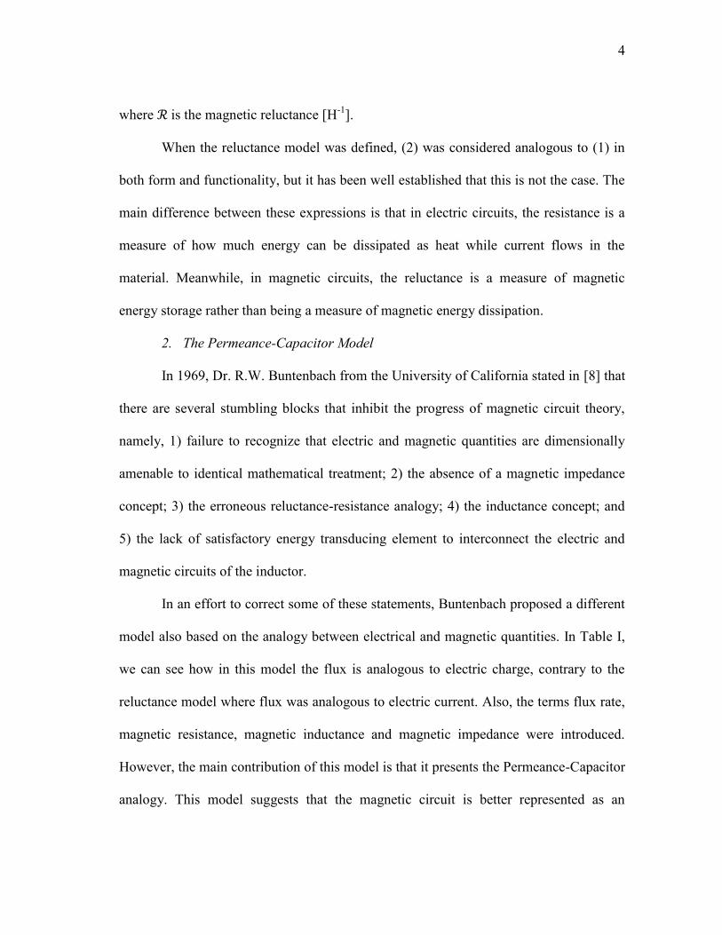
When the reluctance model was defined, (2) was considered analogous to (1) in

both form and functionality, but it has been well established that this is not the case. The

main difference between these expressions is that in electric circuits, the resistance is a

measure of how much energy can be dissipated as heat while current flows in the

material. Meanwhile, in magnetic circuits, the reluctance is a measure of magnetic

energy storage rather than being a measure of magnetic energy dissipation.

2. The Permeance-Capacitor Model

In 1969, Dr. R.W. Buntenbach from the University of California stated in [8] that

there are several stumbling blocks that inhibit the progress of magnetic circuit theory,

namely, 1) failure to recognize that electric and magnetic quantities are dimensionally

amenable to identical mathematical treatment; 2) the absence of a magnetic impedance

concept; 3) the erroneous reluctance-resistance analogy; 4) the inductance concept; and

5) the lack of satisfactory energy transducing element to interconnect the electric and

magnetic circuits of the inductor.

In an effort to correct some of these statements, Buntenbach proposed a different

model also based on the analogy between electrical and magnetic quantities. In Table I,

we can see how in this model the flux is analogous to electric charge, contrary to the

reluctance model where flux was analogous to electric current. Also, the terms flux rate,

magnetic resistance, magnetic inductance and magnetic impedance were introduced.

However, the main contribution of this model is that it presents the Permeance-Capacitor

analogy. This model suggests that the magnetic circuit is better represented as an

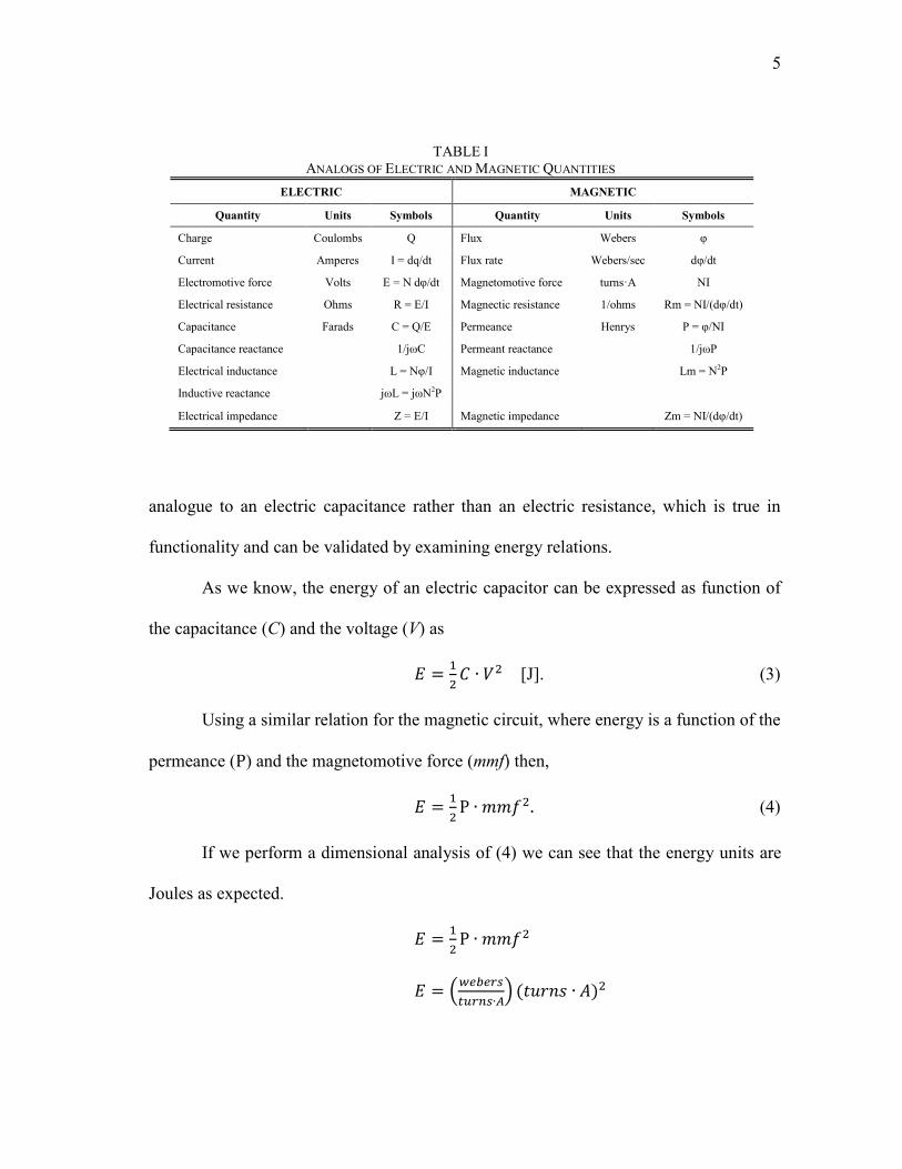
5

analogue to an electric capacitance rather than an electric resistance, which is true in

functionality and can be validated by examining energy relations.

As we know, the energy of an electric capacitor can be expressed as function of

the capacitance (C) and the voltage (V) as

[J]. (3)

Using a similar relation for the magnetic circuit, where energy is a function of the

permeance ( ) and the magnetomotive force (mmf) then,

(4)

If we perform a dimensional analysis of (4) we can see that the energy units are

Joules as expected.

(

)

TABLE I

ANALOGS OF ELECTRIC AND MAGNETIC QUANTITIES

ELECTRIC MAGNETIC

Quantity Units Symbols Quantity Units Symbols

Charge Coulombs Q Flux Webers φ

Current Amperes I = dq/dt Flux rate Webers/sec dφ/dt

Electromotive force Volts E = N dφ/dt Magnetomotive force turns·A NI

Electrical resistance Ohms R = E/I Magnectic resistance 1/ohms Rm = NI/(dφ/dt)

Capacitance Farads C = Q/E Permeance Henrys P = φ/NI

Capacitance reactance

1/jωC Permeant reactance

1/jωP

Electrical inductance

L = Nφ/I Magnetic inductance

Lm = N2P

Inductive reactance

jωL = jωN2P

Electrical impedance Z = E/I Magnetic impedance Zm = NI/(dφ/dt)

6

. (5)

3. The Gyrator-Capacitor Model

In 1993, Dr. D. Hamill applied a method similar to [8] to model magnetic

circuits. He applied the gyrator-capacitor approach to model: a gapped-core inductor, a

two-winding transformer and a Ćuk converter with satisfactory results [9, 10].

In the Gyrator-Capacitor model, the permeance is used analogous to the electric

capacitance, but as seen in Table II, it is the only circuit quantity of the model, contrary

to the Permeance-Capacitor model which includes expressions for magnetic resistance

and inductance. However, in later publications appear extensions to the original gyrator-

capacitor model where a magnetic resistance and magnetic inductance are defined but

there is neither a comprehensive description nor an application of them [11, 12].

The quantities of the gyrator-capacitor model are based on the gyrator theory [13,

TABLE II

GYRATOR-CAPACITOR MODEL ANALOGIES

Magnetic Circuit Electrical Circuit

Quantity Units Symbols Quantity Units Symbols

MMF A mmf Voltage V v

Flux rate V dφ/dt Current A i

Permeance H Capacitance F C

Flux Wb φ Charge C ∫

Permeability H/m Permittivity F/m

Power W Power W

Energy J ∫ Energy J ∫

7

14]. The gyrator, first introduced by Tellegen in 1948, is a two-port network passive

element that links the electric and magnetic regimes.

In Chapter III, we will explain in detail the gyrator as it will be used to define the

quantities that we propose for our model.

C. Problem

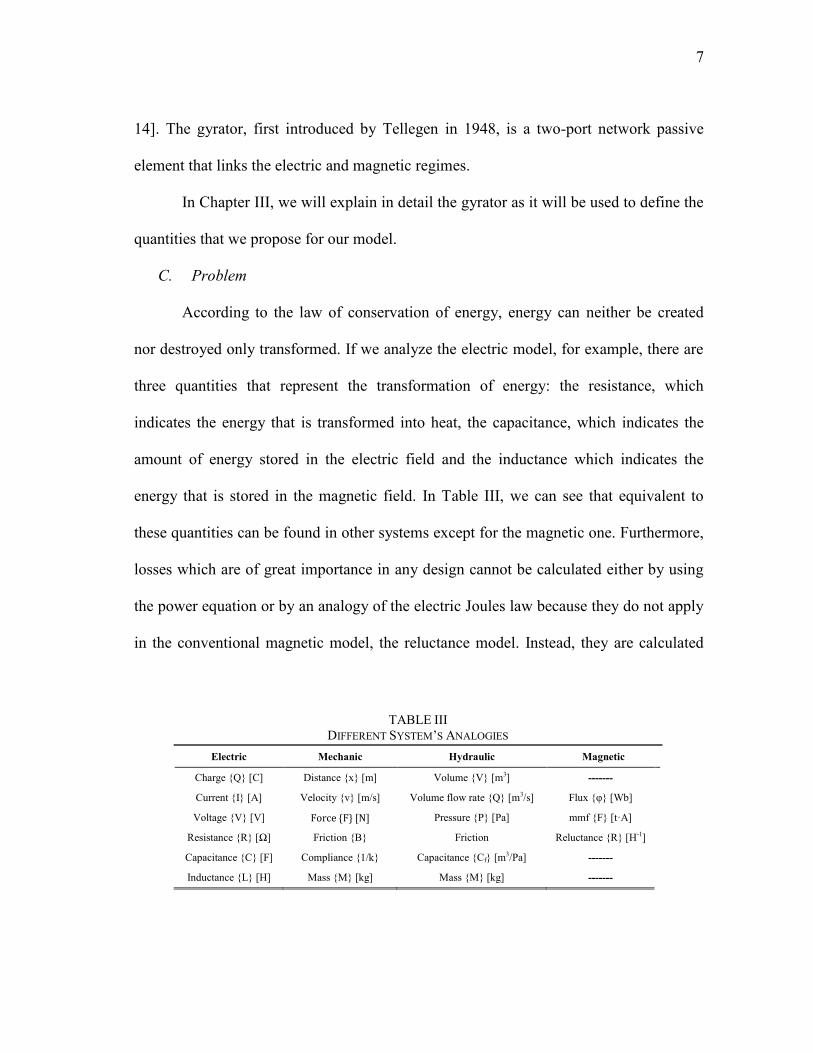
According to the law of conservation of energy, energy can neither be created

nor destroyed only transformed. If we analyze the electric model, for example, there are

three quantities that represent the transformation of energy: the resistance, which

indicates the energy that is transformed into heat, the capacitance, which indicates the

amount of energy stored in the electric field and the inductance which indicates the

energy that is stored in the magnetic field. In Table III, we can see that equivalent to

these quantities can be found in other systems except for the magnetic one. Furthermore,

losses which are of great importance in any design cannot be calculated either by using

the power equation or by an analogy of the electric Joules law because they do not apply

in the conventional magnetic model, the reluctance model. Instead, they are calculated

TABLE III

DIFFERENT SYSTEM’S ANALOGIES

Electric Mechanic Hydraulic Magnetic

Charge Q [C] Distance x [m] Volume V [m3] -------

Current I [A] Velocity v [m/s] Volume flow rate Q [m3/s] Flux φ [Wb]

Voltage V [V] Force F [N] Pressure P [Pa] mmf F [t·A]

Resistance R [Ω] Friction B Friction Reluctance R [H-1]

Capacitance C [F] Compliance 1/k Capacitance Cf [m3/Pa] -------

Inductance L [H] Mass M [kg] Mass M [kg] -------

8

using empirical equations or most commonly, by using the area of hysteresis loops as in

the case of the hysteresis loss calculation.

In this dissertation, we will present an alternative model to magnetic systems that

seeks to standardize the models in all regimes and show an elegant solution to the power

calculation problem. Our approach is different to the models discussed earlier because

we believe that the macroscopic magnetic phenomena can be represented by three

quantities (magnetic resistance, inductance and capacitance) of magnetic origin, not just

as quantities gyrated from the electric to the magnetic regime. Nevertheless, we

understand that this model has limitations and we must be very careful in its

characterization to avoid any misconceptions.

D. Research Objectives

Using gyrator theory and knowing that power is invariant across different energy

regimes, we will:

Standardize the magnetic system model;

Develop a method of modeling magnetic systems using lumped parameters;

Use techniques, well known in other regimes, to analyze magnetic systems;

Use our new models to facilitate the design, study, and simulation of complex

magnetic systems;

Use our new modeling insights to invent new magnetic systems.

9

E. Dissertation Organization

The next chapter includes a literature review of magnetic materials and

electromagnetic theory as these are fundamental for the development of the theory that

we are proposing.

In Chapter III, we present our theory. It offers a comprehensive description of all

the quantities used in our model which are defined based on an analogy between electric

and magnetic regimes.

In Chapter IV we present a conceptual test that was designed with the purpose of

finding the configuration of magnetic elements that represents the behavior of an iron

core coil used as case study. Also, we elaborate a conceptual experiment using

Simulink® in order to validate our model.

The core of Chapter V is the application of our theory. We explore the idea of

transmitting power in the magnetic regime using a novel concept that we have

denominated a magnetic transmission line. We design a case study system where the

electric terminals parameters and the magnetic characteristics of the line are given. The

optimal design is chosen based on how the efficiency and the power factor of the system

are affected due to variations in geometry, frequency and the number of turns of the

windings.

Finally, Chapter VI will summarize the work accomplished and propose future

research in this area of knowledge.

10

CHAPTER II

LITERATURE REVIEW

Since the discovery of the loadstone and its application in devices like the

navigational compass, invented around 1088 in China, different theories have been

developed in order to explain the magnetic phenomena and the properties of magnetic

materials. This chapter presents a literature review of the most significant contributions

made to this area of knowledge.

A. Fundamentals of Electromagnetism

1. The Law of Force between Particles

In physics, the interactive forces are the ways that the simplest particles in the

universe interact with one another. The four known interactive forces are strong

interaction, weak interaction, gravitation and electromagnetism [15].

Gravitation was the first force to be known that affect all material particles. In

1687, Sir Isaac Newton postulated the inverse-square law of universal gravitation which

states that the gravitational attraction between two masses (m1, m2) varies inversely as

the square of the distance (r) between them,

[N]. (6)

In the 18th

century, when electromagnetism was considered as two different

forces: electricity and magnetism, it occurred to the pioneers of electricity that the force

between electrically charged particles might obey the same rules as gravitation.

Experimental verification of this theory was announced in 1785 by Charles Coulomb

11

[16]. The Coulomb’s inverse square law, also known as Coulomb’s law, states that the

force between two particles at rest is proportional to the product of their charges (q1, q2),

and inversely proportional to the square of the distance (r) between them,

[N]. (7)

Charges with same polarity repeal each other while charges with different polarities

attract each other. A similar behavior was seen in magnetism.

Almost everyone as a child has played with magnets and felt the mysterious

forces of attraction and repulsion between them. These forces appear to originate in

regions called poles, located near the ends of the magnet. Two independent studies, one

made by John Michell in England in 1750 and the other by Charles Coulomb in France

in 1785, showed that the forces between the extremities or poles of two magnets obeyed

the inverse square law [17, 18].

In this case, the force between two magnetic poles is proportional to the product

of their pole strengths (p1, p2) and inversely proportional to the square of the distance (r)

between them,

[N]. (8)

Nevertheless, in (8) different to (7) a single magnetic pole (pi), which should be

analogous to an electric charge (qi), does not exists. Physicist that tried to separate the

poles of a magnet obtained, not a pair of single poles, but a pair of magnets. It became

apparent that the ultimate indivisible unit of magnetism was not the magnetic charge but

a magnetic dipole, which might consist of a pair of equal and opposite magnetic charges

indissolubly, fixed together. However, despite the fact that magnetic poles represent a

12

mathematical concept rather than reality, the concept is useful in visualizing many

magnetic interactions, and helpful in the solution of magnetic problems.

2. Electric and Magnetic Fields

In the same way as the Earth is considered to be surrounded by a gravitational

field in which heavy bodies experience forces, the electric charges (qi) are said to be

surrounded by an electric field, which is a region in space or matter in which a charged

particle experiences a force. This force is directly proportional to the product of the

charge (q) and the electric field intensity (E),

[N]. (9)

The electric field intensity (E) is one of the vector quantities used to describe the electric

field. The second vector quantity that is used to describe the electric field is the electric

flux density or displacement field (D). The primary function of the vector D is to give a

point-by-point description of the field that is independent of the character of the

medium, different to the vector E which is dependent of the medium,

[C/m2], (10)

where ε is the dielectric constant of the medium [F/m].

The electric field intensity, the electric flux density and the electric force are

vectors that possess the same direction. As we cannot see the electric field, we form a

mental picture of it using the idea of lines of force. A line of force is a continuous curve,

whose direction at every point is that of the electric field. For example, in Fig. 1a, the

electric field is depicted as lines of force flowing from two opposite charges.

13

Similar to the electric regime, in the magnetic regime the magnetic pole creates a

magnetic field, and is this field which produces a force on a second pole nearby [18].

Experiment shows that this force is directly proportional to the product of the pole

strength (p) and the field intensity (H),

[N]. (11)

Fig. 1b shows the magnetic field as lines of force emanating from a bar magnet. By

convention the lines originate at the north pole and end at the south pole.

The magnetic field intensity (H) is one of the vector quantities used to describe

the magnetic field. The second vector quantity that is used to describe the magnetic field

is the magnetic flux density or magnetic induction (B). In this case, the vector H is

independent of the character of the medium while the vector B is dependent of the

medium,

[Wb/m2], (12)

where µ is the permeability of the medium [H/m].

Fig. 1. Electric and magnetic fields depicted by lines of force.

14

The magnetic field intensity, the magnetic flux density and the magnetic force

are vectors that possess the same direction. In cases where the material is anisotropic, the

permeability is considered as a vector as well, and the magnetic field intensity and the

magnetic flux density do not share the same direction.

In 1865, James Clerk Maxwell presented a set of differential equations that

described the relationship that exists between the electric and magnetic fields,

. (13)

Basically, they describe how electric charges and electric currents are the sources of

electric and magnetic fields. These equations are a compendium of Gauss’s, Faraday’s

and Ampere’s laws and are the core of electromagnetism.

3. Electric and Magnetic Moments

When positive and negative charges in a material are in the presence of an

electric field, they tend to be displaced a finite distance (d) relative to each other creating

an electric dipole moment (pe) as depicted in Fig. 2. This moment can be expressed as,

. (14)

The macroscopic dipole moment density (Pe) is given by

, (15)

where n is the number of microscopic electric dipole moments/volume.

15

The dipole moment density (Pe) is related to the electric field through the electric

susceptibility (χe), which is a measure of how easily a material is polarized in the

presence of an electric field [19]. This relation can be expressed as,

. (16)

The relationship between the electric field, the dipole moment density and the

electric flux density, in this case also known as electric displacement field, can be

expressed in terms of the permittivity of the medium (ε) as,

. (17)

On the other hand, in the magnetic regime, the magnetic moment (m) is

considered the elementary quantity in solid-state magnetism and can be defined as a

quantity that determines the force that a magnet can exert on either a bar magnet or a

current loop when it is in an applied field. It can be expressed in terms of a magnetic

pole as,

, (18)

Fig. 2. Electric dipole: two opposite charges separated by a finite distance.

16

where m is the magnetic moment, p is the magnetic pole strength and d is the distance

between the poles.

In 1850 Hans Cristian Oersted discovered that an electric current produced a

magnetic field in its neighborhood. The nature of this phenomenon was fully explored

by André Ampère and Wilhelm Eduard Weber. They showed that a current loop was

magnetically equivalent to a dipole, fixed at the center of the circuit and perpendicular to

its plane (see Fig. 3). This hypothesis agrees with modern physical theory that believes

that an electron spin, a nuclear spin and atomic orbits with their circling electrons may

be considered as tiny loops of currents. Therefore, the ultimate source of any magnetic

field most truly be regarded, not as a small bar magnet, but as a small loop of current [1].

This implies that the magnetic moment can also be described in terms of a current (I)

flowing in a tiny loop of area A as,

. (19)

Fig. 3. Sources of magnetic moment.

17

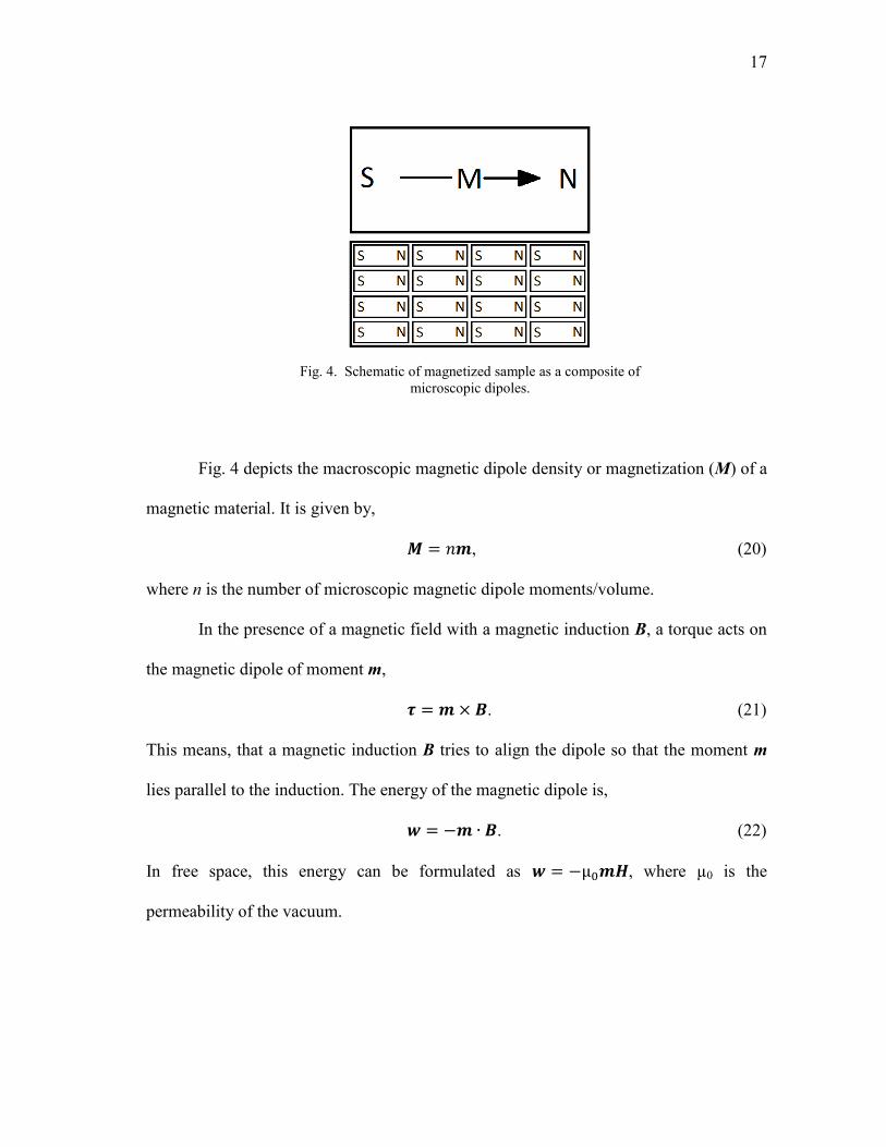
Fig. 4 depicts the macroscopic magnetic dipole density or magnetization (M) of a

magnetic material. It is given by,

, (20)

where n is the number of microscopic magnetic dipole moments/volume.

In the presence of a magnetic field with a magnetic induction B, a torque acts on

the magnetic dipole of moment m,

. (21)

This means, that a magnetic induction B tries to align the dipole so that the moment m

lies parallel to the induction. The energy of the magnetic dipole is,

. (22)

In free space, this energy can be formulated as , where µ0 is the

permeability of the vacuum.

Fig. 4. Schematic of magnetized sample as a composite of

microscopic dipoles.

18

The magnetization (M) is related to the magnetic field through the magnetic

susceptibility (χm), which is a measure of how easily a material is polarized in the

presence of a magnetic field. This relation can be expressed as,

. (23)

The relationship between the magnetic field intensity, the magnetic flux density

and the dipole moment density can be expressed in terms of the permeability of the

medium (µ) by,

. (24)

B. Magnetization and Magnetic Materials

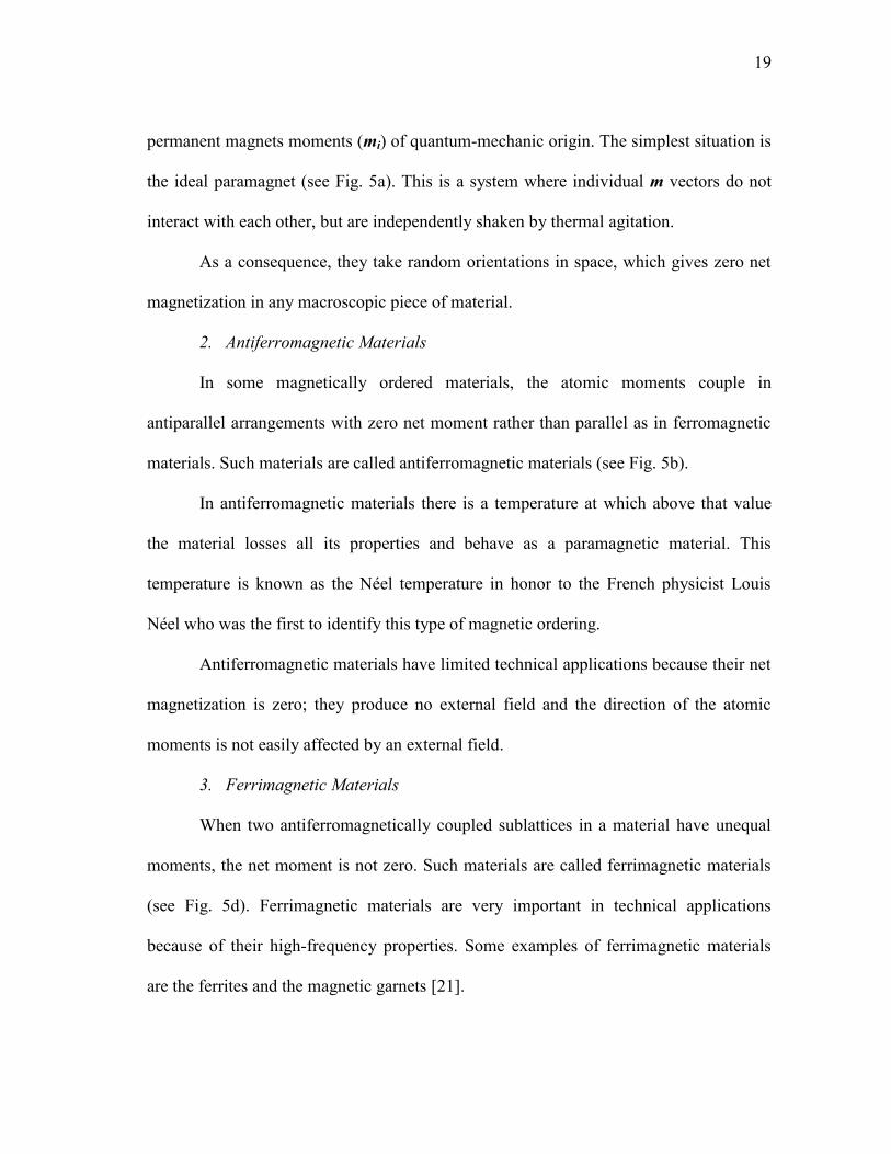
There are four types of magnetic materials: paramagnetic, antiferromagnetic,

ferromagnetic, and ferrimagnetic. The difference between them is the macroscopic

magnetic effect experienced due to the orientation of the atomic magnetic moments in

the presence of a magnetic field (see Fig 5).

1. Paramagnetic Materials

According to [20], a magnetic material can be imagined as an assembly of

Fig. 5. Ordering of the magnetic dipoles in magnetic materials.

19

permanent magnets moments (mi) of quantum-mechanic origin. The simplest situation is

the ideal paramagnet (see Fig. 5a). This is a system where individual m vectors do not

interact with each other, but are independently shaken by thermal agitation.

As a consequence, they take random orientations in space, which gives zero net

magnetization in any macroscopic piece of material.

2. Antiferromagnetic Materials

In some magnetically ordered materials, the atomic moments couple in

antiparallel arrangements with zero net moment rather than parallel as in ferromagnetic

materials. Such materials are called antiferromagnetic materials (see Fig. 5b).

In antiferromagnetic materials there is a temperature at which above that value

the material losses all its properties and behave as a paramagnetic material. This

temperature is known as the Néel temperature in honor to the French physicist Louis

Néel who was the first to identify this type of magnetic ordering.

Antiferromagnetic materials have limited technical applications because their net

magnetization is zero; they produce no external field and the direction of the atomic

moments is not easily affected by an external field.

3. Ferrimagnetic Materials

When two antiferromagnetically coupled sublattices in a material have unequal

moments, the net moment is not zero. Such materials are called ferrimagnetic materials

(see Fig. 5d). Ferrimagnetic materials are very important in technical applications

because of their high-frequency properties. Some examples of ferrimagnetic materials

are the ferrites and the magnetic garnets [21].

20

4. Ferromagnetic Materials

The most common type of magnetic material used in industry nowadays are

ferromagnetic materials. In ferromagnetic materials (Fig. 5c) a nonzero magnetization

can be induced by an external field (Ha).

According to [20], the potential energy of a single moment in the field is equal to

. (25)

This energy term favors the alignment of the moments along the direction of the

field direction. Conversely to the tendency of thermal agitation that just destroys any

order possibly present.

An appreciable net magnetization component along the field is obtained when the

field energy is at least comparable in order of magnitude to the thermal energy. This can

be expressed as,

, (26)

where µ0µBHa represents the field energy and kBT represents the thermal energy. The

constant µB is the natural atomic unit of magnetic moments and is called the Bohr

magneton.

At room temperature, the net magnetization would take place for fields Ha ≈

3x108 A/m which is about 10

6 times bigger than the normally applied (10-10

2 A/m). This

raises the question on how we overcome thermal agitation and produce any appreciable

magnetization.

In 1907, a French physicist Pierre-Ernest Weiss suggested that ferromagnetic

materials could exhibit a large spontaneous magnetization even at low fields because the

21

elementary magnetic moments were by no means independent, as assumed in the

previous picture of paramagnets, but were strongly coupled by an internal field

proportional to the magnetization itself, Hw α M, which he termed molecular field. The

molecular field produces a positive feedback mechanism, because the presence of a net

magnetization produces a nonzero molecular field, which in turn acts on all moments

trying to further align them. The result is that, below a critical temperature, the Curie

temperature (Tc), the magnetic moments spontaneously attain long-range order and the

material acquires a substantial spontaneous magnetization (Ms). The Curie point of a

ferromagnetic material is the temperature above which it loses its characteristic

ferromagnetic ability. Above the Curie point, the material is purely paramagnetic and

there are no magnetized domains of aligned moments. The knowledge of the

experimental value of Tc permits one to estimate the order of magnitude of Hw, because

at the Curie point one expects . In the case of iron, where , one

finds . Well below Tc, the moments are nearly perfectly aligned. In iron at

room temperature, this gives a spontaneous magnetization of the order of 2 T.

The molecular field hypothesis explains the main aspects of the temperature

dependence of the spontaneous magnetization but raises other conceptual difficulties. If

there exists an internal field as enormous as the estimate of 109 A/m seems to indicate,

then one would expect to find ferromagnetic materials spontaneously magnetized to

saturation under all circumstances. Thus how can a hysteresis loop exist at all? It would

seem impossible that fields of the order of 10 A/m can reduce to zero the magnetization

of a ferromagnet if they are confronted with internal fields of the order of 109 A/m.

22

Weiss proposed to resolve this difficulty by postulating that a ferromagnetic

material is subdivided into regions called magnetic domains. In each domain, the degree

of magnetic moment alignment is dictated by the molecular field, but the orientation of

the spontaneous magnetization can vary from domain to domain. As a consequence,

when the magnetization is averaged over volumes large enough to contain many

domains, one obtains values mainly determined by the relative orientation and volume of

domains. The result can be very different from the spontaneous magnetization and even

close to zero. The variety of observed hysteresis loop shapes is the direct consequence of

the variety of possible magnetic domain structures.

4.1. B-H Loops and Magnetic Domains

It has been already explained that a change in magnetic flux density (B) depends

on the values of the magnetic field intensity (H). However, it also depends on the history

of the magnetic material that is, the values of H to which it has been subjected in the

past. It is therefore necessary to specify the magnetic history with some exactness.

In a large number of applications such as motors and transformers, the magnetic

material is exposed to a magnetizing force which alternates between equal positive and

negative values. It is found that after a few of such alternations, the curve connecting B

and H settles down to a cycle which is exactly reproduced in each successive alternation.

The material is then said to be in a cyclic condition and the B-H curve may take the form

shown in Fig. 6 known as hysteresis loop or B-H loop. The name hysteresis is given due

to the lag between cause and effect [22].

23

The features of the loops may be explained with the help of the domain theory.

Consider a magnetic material in the demagnetized state, this is B=0 and H=0. According

to [1], if we apply a field that rises from zero to Hmax, the application of the weak field

produces motion of domain walls such as to expand the volume of those domains having

the largest component of M along H. The initial induction B produced in response to a

small field H defines the initial permeability. At higher fields H, B increases sharply and

the permeability increases to its maximum. When most domain wall motion has been

Fig. 6. Hysteresis loop of a magnetic material. The approximate domain structures are indicated at right

for demagnetized state and for approach saturation.

24

completed, there often remains domains with nonzero components of magnetization at

rigth angles to the applied field direction. The magnetization in these domains must be

rotated into the field direction to minimize potential energy –M·B. This process

generally costs more energy than wall motion because it involves rotating the

magnetization away from an easy direction. When the applied field is of sufficient

magnitude that these two processes, wall motion and magnetization rotation are

complete, the sample is in a state of magnetic saturation Bs = µ0(H+Ms).

On decreasing the magnitude of the applied field, the magnetization rotates back

towards its easy direction, generally without hysteresis (i.e., rotation is a largely

reversible, lossless process). As the applied field decreases further, domain walls begin

moving back across the sample. Because energy is lost when a domain wall jumps

abruptly from one local energy minimum to the next (Barkhausen jumps), the hysteresis

loop opens up. That is, it shows hysteresis.

When the hysteresis loops of different materials are compared, some of the

properties are denoted by special terms. The usually accepted definitions of these terms

are as follows:

Remanence is the flux density or magnetic induction, which remains in a

magnetic material after the removal of an applied magnetizing force.

Residual flux density or residual induction (Br), in a magnetic material is the

value of the flux density for the condition of zero magnetizing force, when the

material is being symmetrically cyclically magnetized. It is distinguished from

the Remanence by the symmetrically cyclic requirement.

25

Retentivity is the flux density that remains in the material after a magnetizing

force sufficient to cause saturation flux density or saturation induction has been

removed.

Coercive force (Hc) of a magnetic material is the magnitude of the magnetizing

force at which the flux density is zero when the material is being symmetrically

cyclically magnetized.

Coercivity is the coercive force required to reduce the flux density in the material

to zero from a condition corresponding to saturation flux density or saturation

induction.

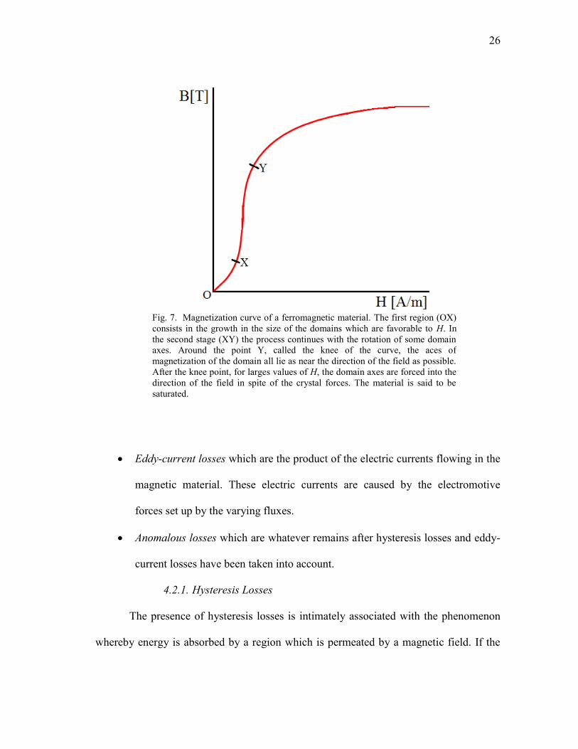
If hysteresis loops are measured for different amplitudes of H, the locus of the

tips of the loops is known as the magnetization curve, saturation curve or B-H

normalized curve (see Fig. 7). The relation between B and H is the permeability (µ) and

can be calculated using the magnetization curve.

4.2. Magnetic Losses

When an electromagnetic device is excited with a constant electric current, the

magnetic flux produces insignificant energy losses unless it is energized and de-

energized very frequently. On the other hand, when devices like motors, transformers,

reactors, etc., are excited with an alternating electric current, the alternating fluxes in the

magnetic material generate heat and therefore, energy losses.

Mainly, there are three types of losses in magnetic materials namely,

Hysteresis losses which are heat losses result of the tendency of the material to

retain magnetism or to oppose a change in magnetism.

26

Eddy-current losses which are the product of the electric currents flowing in the

magnetic material. These electric currents are caused by the electromotive

forces set up by the varying fluxes.

Anomalous losses which are whatever remains after hysteresis losses and eddy-

current losses have been taken into account.

4.2.1. Hysteresis Losses

The presence of hysteresis losses is intimately associated with the phenomenon

whereby energy is absorbed by a region which is permeated by a magnetic field. If the

Fig. 7. Magnetization curve of a ferromagnetic material. The first region (OX)

consists in the growth in the size of the domains which are favorable to H. In

the second stage (XY) the process continues with the rotation of some domain

axes. Around the point Y, called the knee of the curve, the aces of

magnetization of the domain all lie as near the direction of the field as possible.

After the knee point, for larges values of H, the domain axes are forced into the

direction of the field in spite of the crystal forces. The material is said to be

saturated.

27

region is other than a vacuum, only a portion of the energy taken from the electric circuit

is stored and is wholly recoverable from the region when the magnetizing force is

removed. The rest of the energy is converted into heat as a result of work done on the

material when it responds to the magnetization [23].

The magnitude of the energy absorbed per unit volume is given as,

[J/m3]. (27)

The addition of this differential energy represents the area inside a B-H loop (Aloop).

The rate at which the energy is dissipated because of hysteresis, also known as

hysteresis power loss, can be calculated using (28) if a volume (V) of magnetic material

has a uniform flux distribution and is subject to a cyclic change at a frequency ( f )

cycles per second.

[W]. (28)

According to [23], Steinmetz found from a large number of measurements that

the area of the normal hysteresis loop of specimens of various irons and steels

commonly used in the construction of electromagnetic apparatus of his day was

approximately proportional to 1.6th

power of the maximum flux density throughout the

range of flux densities from about 0.1 to 1.2 T. Advances on ferromagnetic

manufacturing have widely transformed and improved the material’s properties since

Steinmetz originally performed his measurements. Therefore, the exponent 1.6 fails

nowadays to give the area of the hysteresis loops with a sufficient degree of accuracy to

be useful. However, the empirical expression for the energy loss per unit volume per

cycle is more properly given as

28

[J/m

3], (29)

where η and n have values that depend on the material. Equation (29) should be used

with caution since the value for n, which may range between 1.5 and 2.5 for present day

materials, may not be a constant value for a given material.

The total hysteresis loss in a volume V in which the flux density is uniform and

varying cyclically at a frequency of f cycles per second can then be expressed

empirically as,

[W]. (30)

4.2.2. Eddy-current Losses

According to Faraday, an induced electromotive force (emf) results within a

magnetic medium due the presence of a time-varying magnetic field. When the medium

is conductive, an electric current appears (see Fig. 8). These currents are called eddy-

currents (ie) and their presence results in an energy loss in the material proportional to

ie2Re, called eddy-current loss.

Fig. 8. Eddy-currents in a transformer core, a) representation of a laminated transformer, b) eddy-

currents in a solid core, c) eddy-currents in a laminated core.

29

Since the flux density in ferromagnetic materials is usually relatively large and

the resistivity is relatively small, the electromotive force, the eddy-currents and the

eddy-current loss may become appreciable if means to minimize them are not taken.

This loss can be minimized by using thin laminations or highly resistive material.

Eddy-current loss is of considerably importance in determining the efficiency,

the temperature rise, and hence the rating of electromagnetic apparatus in which the flux

density varies.

In a magnetic circuit containing a volume V of laminated core material exposed

to a sinusoidal flux, the average eddy-current power loss is,

[W], (31)

where, V is expressed in m3, f in Hz, the thickness of the lamination (τ) in meters, Bmax

in Teslas, and ρ in ohms/m3.

Another phenomenon that is linked to the eddy-currents is skin effect. The effect

of such currents is to screen or shield the material from the flux, and to bring about a

smaller flux density near the center of the slab than at the surface. This is, similar to the

skin effect observed in electric conductors [23].

Since electric and magnetic skin effects are similar in nature, they are subject to

the same type of analysis and solution. In electric circuits, the effect is mitigated using a

number of insulated wire strands woven together in a carefully designed pattern instead

of using a solid conductor. In magnetic circuits, we apply the same strategy. The skin

effect is mitigated by laminating the core, thus reducing the eddy-currents.

30

4.2.3. Anomalous Losses

According to [2], anomalous losses are the remaining losses after hysteresis and

eddy-current losses have been taken into account. They turn out to be comparable in

magnitude to eddy-current losses and they arise from extra eddy-current losses due to

domain wall motion, non-uniform magnetization and sample inhomogeneity. Essentially,

the anomalous losses reflect the broadening of the hysteresis loop with increasing

frequency, so the separation of static hysteresis loss and anomalous loss is artificial.

31

CHAPTER III

POWER-INVARIANT MAGNETIC MODEL

In all energy systems, the parameters necessary to calculate power are the same

in functionality, an effort or force needed to create a movement in an object and a flow

or rate at which the object moves [24]. Therefore, we can generalize the power equation

as a function of these two parameters: effort and flow,

. (32)

Analyzing various power transfer media this is true for at least three regimes:

electrical, mechanical and hydraulic but not for magnetic (see Table IV). This implies

that the conventional magnetic system model (the reluctance model) requires

modifications in order to be consistent with other energy system models.

Even further, if we do a comprehensive comparison among the systems, each

system’s model includes an effort quantity, a flow quantity and three passive elements

used to establish the amount of energy that is stored or dissipated as heat. After

evaluating each one of them, it was clear that the conventional magnetic model did not

follow the same pattern: the reluctance, seen as an analogy of the electric resistance,

TABLE IV

CALCULATION OF POWER IN DIFFERENT REGIMES

Electric Mechanic Hydraulic Magnetic

Voltage x Current Force x Velocity Pressure x Flow MMF x Flux

V x A N x m/s N/m2 x m3/s A x Wb

Watts Watts Watts Joules

32

does not dissipate energy, but instead stores energy and the two other elements are not

defined (see Table V). This difference has initiated a reevaluation of the conventional

magnetic model.

A. The Power Equation

As we established earlier, the power equation in the reluctance model is not

satisfied. This implies that either the magnetic effort (mmf) or the magnetic flow (flux) is

not properly defined. According to [8], the gyrator is the missing link that can help us

find the proper definition of these quantities.

A symbolic representation of the conventional gyrator is presented in Fig. 9. It is

TABLE V

FUNDAMENTAL QUANTITIES OF DIFFERENT SYSTEM’S MODELS

Quantities Electric Mechanic Hydraulic Magnetic

Conserved Quantity Charge [C] Distance [m] Volume [m3] -------

Flow Current [A] Speed [m/s] Volume flow rate [m3/s] Flux [Wb]

Effort Voltage [V] Force [N] Pressure [Pa] MMF [t·A]

Dissipative Element Resistance [Ω] Friction Friction Reluctance [H-1]

Energy Storage Element Capacitance [F] Compliance Capacitance [m3/Pa] -------

Energy Storage Element Inductance [H] Mass [kg] Mass [kg] -------

Fig. 9. Symbolic representation of a two-port gyrator.

33

a two-port network passive element that converts the effort or flow quantity into its dual

with respect to its gyration constant (g), this is

, (33)

. (34)

This conversion is lossless. Therefore, the power at the terminals of both

networks is invariant,

. (35)

This characteristic is very important in cases where only one of the two networks is

known as it provides valuable information of the unknown network.

The gyrator was developed on the basis that there should exist a complement to

the ideal transformer which is a two-port network passive element as well, but in which

the effort and flow quantities must follow the reciprocity property. This is,

(36)

(37)

where k is a transformation coefficient [25].

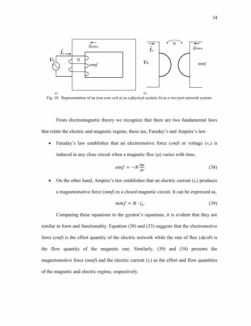
Fig. 10 presents an iron core coil. It can be considered a gyrator as it is a two-port

network system where the primary network is at the electric regime and the secondary

network is at the magnetic regime. Both networks are interconnected through the

winding and its number of turns (N) serve as the gyrator constant. We will use this case

study along this dissertation in order to characterize the magnetic network which at this

point we consider unknown.

34

From electromagnetic theory we recognize that there are two fundamental laws

that relate the electric and magnetic regime, these are, Faraday’s and Ampère’s law.

Faraday’s law establishes that an electromotive force (emf) or voltage (ve) is

induced in any close circuit when a magnetic flux (φ) varies with time,

. (38)

On the other hand, Ampère’s law establishes that an electric current (ie) produces

a magnetomotive force (mmf) in a closed magnetic circuit. It can be expressed as,

. (39)

Comparing these equations to the gyrator’s equations, it is evident that they are

similar in form and functionality. Equation (38) and (33) suggests that the electromotive

force (emf) is the effort quantity of the electric network while the rate of flux (dφ/dt) is

the flow quantity of the magnetic one. Similarly, (39) and (34) presents the

magnetomotive force (mmf) and the electric current (ie) as the effort and flow quantities

of the magnetic and electric regime, respectively.

Fig. 10. Representation of an iron core coil a) as a physical system, b) as a two port network system.

35

In order to verify that these quantities satisfy the power equation, we perform a

dimensional analysis. In (40) we can see that using the electromotive force (mmf) as

magnetic effort and the rate of flux (dφ/dt) as magnetic flow in the power equation, it

gives watts units;

, (40)

where t is a dimensionless unit that represents the number of turns of the winding.

Using the rate of magnetic flux (dφ/dt) as flow is the fundamental modification to

the reluctance model. It is the key to define the rest of the parameters (magnetic

resistance, inductance and capacitance) needed to standardize the magnetic model.

B. Magnetic Fundamental Quantities

After studying different regimes we realized that there are six fundamental scalar

quantities needed to fully model any energy transfer process. They can be generalized as,

conserved quantity, effort, flow, dissipative element and two energy storage elements,

one that stores energy due to effort and the other that stores energy due to flow.

In this section we define these quantities for the magnetic regime. We use an

electric analogy as basis to derive the magnetic model, first, because there is an intrinsic

relation between both systems and second, we are familiar with electric circuit theory.

36

1. Conserved Quantity

In general terms we can define the conserved quantity as the fundamental

physical entity of a system. Depending on the regime of work it has different

designations, for example, in mechanic systems it is the distance (m), in fluid dynamics

is the mass (kg), in hydraulics it is the volume (m3) and in electric systems is the electric

charge (C). In order to define the magnetic conserved quantity we will present a

description of the electric conserved quantity as it will be used as analogous to the

magnetic one.

1.1. Electric Conserved Quantity

In electric systems, the free charge (qe) is usually considered the conserved

quantity. However, this is not the general case, depending on the media at which a

process takes place the interpretation of the electric conserved quantity may vary. For

instance, in free space or in a conductive media, like a metallic conductor, the free

charge is considered the conserved quantity. It iteration with an electromagnetic field or

with other charged particles is the main cause of the electric phenomena.

In dielectric materials, on the other hand, due to the tight atom-electron bonds

there are no free charges. The electric phenomenon is the result of the interaction of

electric fields and the polarized charges of the dielectric material. These charges, which

are basically electric dipoles, are known as bound charges to distinguish them from the

free charges.

As we explain in Chapter II, the dipoles are two opposite charges. Therefore, the

average electric bound charge in a closed surface (S) at rest is zero. However, when a

37

dielectric is excited with an electric field (E), these charges get polarized and its effect

can be appreciated in the displacement field. The scalar quantity that represents this

effect is the electric flux (ψ) and it is expressed as,

∮ ∮ . (41)

Karl Friedrich Gauss established that the total flux out of any closed surface of

area (S) is equal to the total charge enclosed by the surface [26]. It is expressed as,

∮ ∑ [C]. (42)

This means that each coulomb of free charge produces a unit of flux (ψ). Therefore, as

these quantities are equivalent we will consider the electric flux as the conserved

quantity when analyzing dielectric materials.

1.2. Magnetic Conserved Quantity

In magnetic materials there are no magnetic free charges since such charges have

not been discovered. As we explain earlier, the minimal magnetic quantity is the

magnetic dipole. We can infer that there is an analogy between the electric dipoles or

bound charges in a dielectric material and the magnetic dipoles of the magnetic material.

In order to be consistent with this analogy, we are going to refer to the magnetic dipoles

as magnetic bound charges.

Similar to the electric case, the magnetic dipoles have opposite polarities.

Therefore, the average magnetic bound charge in a closed surface (S) at rest is zero.

Nevertheless, when a magnetic material is excited with a magnetic field (H), these

charges get magnetized and its effect can be appreciated in the magnetic flux density.

38

The scalar quantity that represents this effect is the magnetic flux (φ) and it is expressed

as,

∫

∫

[Wb]. (43)

Similar to the electric flux considered as an electric conserved quantity, we will

use the magnetic flux (φ) as the magnetic conserved quantity. In order to be consistent

with the electric analogy, we will refer indistinctively to the magnetic conserved quantity

in terms of the flux (φ) or as a bound charge (qm).

It is important to point out that the previous interpretation of magnetic flux as

conserved quantity was obtained following an analogy between electric and magnetic

systems. Furthermore, it is consistent with the conserved quantity expected from the

integration of the magnetic flow obtained using gyrator theory. This is,

∫ [Wb]. (44)

As the magnetic flow is the rate of magnetic flux (

), then the conserved quantity

is again the magnetic flux (φ).

2. Flow

The flow can be generalized as the movement of the conserved quantity through

certain area per unit of time. Depending on the regime of work it has different

designations, for example, in mechanics systems it is known as speed (m/s), in fluid

dynamics is known as mass flow (kg/s), in hydraulics it is called volumetric flow rate

(m3/s) and in electric systems it is called electric current (C/s). In order to define the

magnetic current we will present a description of the electric current as it will be used as

analogous to the magnetic one.

39

2.1. Electric Current

Electric currents are divided in two classes, conduction currents and

displacement currents. Conduction currents result from the movement of charged

particles in a conductive medium. The motion of these particles generates heat and

therefore, it is usually associated with energy losses.

Mathematically it is given by,

[A]. (45)

Displacement currents were introduced by James Clerk Maxwell in 1861 in order

to satisfy Ampère’s circuital law which establishes that currents always flow in a closed

path. It answers the current through capacitors as there are no free charges moving inside

the dielectric medium. Mathematically it is given by

[A], (46)

where ψ is used to denominate the electric flux [C].

Displacement currents are not based on the movement of free charged particles

but instead in the rate of change of electric fields. However, they are recognized as a

moving-charge current related to the bound or polarized charge of a dielectric material.

Displacement currents play little role in metallic conduction. In metals they are

dwarf into insignificance by the magnitude of the conductive current; but in insulators

where the conduction currents are weak, the displacement current may well play a role

even at low frequencies and most certainly when the frequencies are elevated [27].

Another way to express the electric current, both the conduction current and the

displacement currents is in terms of its current density (Je),

40

[A/m

2]. (47)

Je is a vector quantity that contains microscopic information regarding the current flow.

In case of the conductive current it is given by,

[A/m2], (48)

where σe represents the electric conductivity which is the inverse of the electric

resistivity ρe. On the other hand, in case of the displacement current it is expressed as,

[A/m

2], (49)

where σe is the electric conductivity of the material [Ω-1

/m], E is the electric field [V/m]

and D is the electric flux density [C/m2].

2.2. Magnetic Current

In magnetic circuits, due to the similarity between the dielectric and the magnetic

material, this is both need to be polarized, we think that the magnetic current should be

defined as a magnetic displacement current. In fact, the expression of flow obtained from

the iron core coil as a gyrator suggests that

[Wb/s], (50)

which is similar in form, functionality and origin to (46) as both are based on flux. In

this case φ is used to denominate the magnetic flux.

Similar to electric displacement currents, the magnetic displacement currents are

not based on the movement of magnetic free charged particles as the existence of such

charges have not been discovered. Instead, they are based in the rate of change of

magnetic fields. However, the displacement currents can be recognized as a moving-

41

charge current related to the movement of the magnetic dipoles during the magnetization

of the magnetic material. It is given by (50) or in terms of its current density as,

[T/s], (51)

Since , the magnetic displacement current can also be expressed in

terms of the magnetization as,

[T/s] (52)

3. Effort

In general terms, the effort can be defined as the force needed to generate a flow

or as the force needed to produce work. Depending on the regime of study it has

different designations, for example, in mechanics systems it is known as force (N), in

fluid dynamics and in hydraulics it is called pressure (Pa) and in electric systems it is

called electric voltage (V). In order to define the magnetic effort we will present a

description of the electric voltage as it will be used as analogous to the magnetic one.

3.1. Electric Voltage

In electric systems the effort quantity is most commonly known as voltage (V),

electric potential (Ue) or electromotive force (emf). It is the force needed to move a

charged particle from one point to another while in the presence of an electric field. In

other words, it is the force needed to generate the flow of current. Mathematically,

∫

[V], (53)

where E is the electric field and dl is an element of the path from point A to point B. In

case of a close path, the expression of the emf becomes,

42

∮ [V]. (54)

3.2. Magnetic Voltage

In magnetic systems, the effort quantity has been denominated magnetic

potential (Um) or magnetomotive force (mmf) analogous to the electromotive force. In

this project we will also refer to it as magnetic voltage analogous to electric voltage.

According to [17], it may be defined as the force needed to bring a unit magnetic pole

from one point to another against the magnetic field. Mathematically,

∫

[t·A], (55)

where H is the magnetic field and dl is an element of the path from point A to point B. In

case of a close path, the expression of the mmf becomes,

∮ [t·A] (56)

In our model, we maintain the magnetomotive force as magnetic effort because it

is consistent with gyrator theory. Nevertheless, in order to complete the analogy, the

mmf must also be defined as the force needed to generate a magnetic current. This

statement contradicts the popular knowledge as it is believed that there is no flow of

anything in a magnetic circuit corresponding to the flow of charge in an electric circuit.

However, we have already established that the magnetic current can be considered

product of a moving-charge related to the magnetization of the magnetic dipoles in

magnetic materials, similar to the moving-charge current related to the bound or

polarized charge of an electric insulator. In both cases, an effort is needed to create the

polarization of the bound charges.

43

4. Resistance

As a standard model element, the resistance can be generalized as the quantity

that describes the amount of energy released as heat due to the flow of current in a

material. When an effort is applied, the material allows up to certain degree of flow of

current, the resistance is a measure of this degree. Its generalized expression is,

. (57)

In order to define the magnetic resistance we will present a description of the

electric resistance as it will be used as analogous to the magnetic one.

4.1. Electric Resistance

In electric circuits (57) comes from Ohm’s law. It relates the electric voltage (ve)

and current (ie) flowing through a conductive material,

[Ω]. (58)

As we explain in the general description, the resistance is a measure of the

amount of current the material allows to flow when certain voltage is applied. Therefore,

its value fundamentally depends on the intrinsic property of the material (resistivity or

conductivity) and the geometry (length and area) of the specimen. This is expressed as

∮

∮

∮

∮

[Ω], (59)

where l [m] and S [m2] represents the length and area of the specimen, respectively and

ρe [Ω·m] and σe [Ω

-1/m] represents the resistivity and conductivity of the material.

44

The power dissipated by the resistance is usually calculated using Joule’s law.

This equation uses the root mean square (RMS) values of the current and voltage to

calculate the power and can only be applied when the resistance is a constant value.

[W]. (60)

4.2. Magnetic Resistance

Similarly, in magnetic circuits we can define a magnetic equivalent resistance

based on the general definition. Therefore, it is the quantity that measures the amount of

magnetic current the material allows to flow when certain voltage is applied. It describes

the amount of energy lost as heat.

We can relate the magnetic current (im) and the magnetic voltage (vm) using,

[Ω

-1]. (61)

Nevertheless, its value depends on the intrinsic property of the magnetic material

(magnetic resistivity or magnetic conductivity) and the geometry (length and area) of the

specimen. This is expressed as

∮

∮

∮

∮

[Ω

-1], (62)


ρm [Ω-1

·m] and σm [Ω/m] represents the magnetic resistivity and conductivity of the

magnetic material.

It is important to point out that there is a fundamental difference between the

electric and magnetic resistance and it has its origins in the mechanism that produces the

flow of currents. The electric resistance describes the opposition that the conductive

45

media presents to the flow of free charges. Therefore, it reflects the heat losses due to the

kinetic energy released by the movement of these free charges. However, as we

established earlier, the magnetic currents result from the polarization or magnetization of

the magnetic dipoles in the magnetic material, similar to the displacement electric

currents are the result of the polarization of bound charges in the dielectric material. The

power dissipated as heat is the result of the resistance of the magnetic material to be

magnetized.

In terms of the field densities the magnetic current can also be expressed similar

to (48) as (63) knowing that the magnetic conductivity σm [Ω/m] and consequently the

magnetic resistivity ρm [Ω-1

·m] were introduced in this model to maintain consistency.

[T/s] (63)

The power dissipated by the magnetic resistance can also be expressed in terms

of an analogy to the Joule’s law when the resistance is a constant value. This is,

, (64)

which is the average of the instantaneous power [W].

If the resistance is nonlinear, the power dissipated by the resistance can be

calculated directly by calculating the average of the instantaneous power,

∑

[W]. (65)

5. Capacitance

As a standard model element, the capacitance can be generalized as the quantity

that measures the amount of energy stored in the regime of work due to an applied effort.

Mathematically it is expressed as,

46

, (66)

where qrw stands for conserved quantity in the regime of work.

In order to define the magnetic capacitance we will present a description of the

electric capacitance as it will be used as analogous to the magnetic one.

5.1. Electric Capacitance

In electric systems, the capacitance measures the ability of a body to hold a

charge (qe) due to a given potential (ve). It describes the amount of energy stored in the

electric field. It is expressed as,

[F]. (67)

Similar to the resistance, the capacitance is also a representation of the material.

Therefore, its value depends on the intrinsic property of the dielectric and the geometry

of the specimen. This is expressed as,

∮

∮

∮

∮

[F]. (68)

where l [m] and S [m2] represents the length and area of the specimen, respectively and ε

[F/m] represents the permittivity of the dielectric material, which determines the ability

of a material to polarize in response to an electric field.

To calculate the energy stored by a capacitance of constant value we use,

[J]. (69)

According to [28], in a more general case, the energy stored can be expressed as,

∫ [J]. (70)

47

5.2. Magnetic Capacitance

In magnetic systems, the capacitance measures the ability of a body to store

energy due to a given potential (vCm). It describes the amount of energy stored in the

magnetic field. It is expressed as,

[H]. (71)

Similar to the resistance, the capacitance is also a representation of the material.

Therefore, its value depends on the intrinsic property of the magnetic material

(permeability) and the geometry of the specimen. This is expressed as,

∮

∮

∮

∮

[H]. (72)


µ [H/m] represents the permeability of the material, which determines the ability of a

material to magnetize in response to a magnetic field.

At this point, it is evident that the magnetic capacitance plays the same role as

the permeance in the reluctance model. Therefore, we validate the statement that says

that the permeance and its inverse, the reluctance, are in fact energy storage elements

instead of dissipative elements.

To calculate the energy stored by a capacitance of constant value we use,

[J]. (73)

In a more general case, the energy stored can be expressed either by,

∫ [J], (74)

48

which is proportional to the energy calculated using the area of the B vs. H plot, or by

using the power equation as,

∫

[J] (75)

6. Inductance

As a standard model element, the inductance can be generalized as the quantity

that measures the amount of energy stored in a complementary or dual of the regime of

work due to a flow. Mathematically is expressed as,

, (76)

where qdrw stands for conserved quantity of the dual regime of work.

In order to define the magnetic inductance we will present a description of the

electric inductance as it will be used as analogous to the magnetic one.

6.1. Electric Inductance

In electric systems, the inductance measures the amount of energy stored in the

magnetic field, represented by the magnetic flux, due to the flow of electric current (ie).

It is expressed as,

. (77)

Similar to the resistance, the inductance is also a representation of the material.

Therefore, its value depends on the intrinsic property of the magnetic material

(permeability) and the geometry of the specimen. This is expressed as,

∮

∮ ∮

∮ (

) [H]. (78)

49


µ [H/m] represents the permeability of the material.

To calculate the energy stored by an inductance of constant value we use,

[J]. (79)


∫ [J], (80)

which is proportional to the energy calculated using the area of the B vs. H plot, or by


∫

[J] (81)

6.2. Magnetic Inductance

In magnetic systems, the inductance measures the amount of energy stored in the

electric field, represented by the electric charge, due to the flow of magnetic current (im).

It is expressed as,

. (82)

It can also be expressed in terms of its geometry, length (l) and area (S), and its

permittivity (ε).

∮

∮ ∮

∮ (

) [F] (83)

To calculate the energy stored by an inductance of constant value we use,

[J]. (84)


∫ [J], (85)

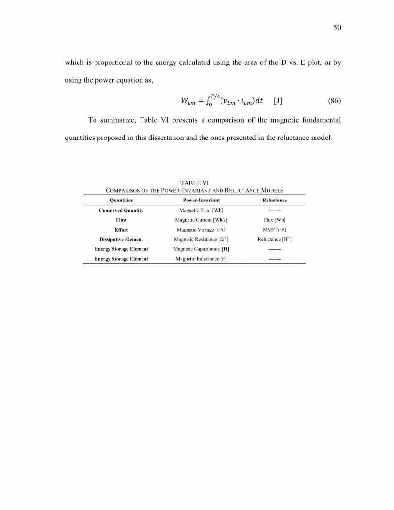
50

which is proportional to the energy calculated using the area of the D vs. E plot, or by


∫

[J] (86)

To summarize, Table VI presents a comparison of the magnetic fundamental

quantities proposed in this dissertation and the ones presented in the reluctance model.

TABLE VI

COMPARISON OF THE POWER-INVARIANT AND RELUCTANCE MODELS

Quantities Power-Invariant Reluctance

Conserved Quantity Magnetic Flux [Wb] -------

Flow Magnetic Current [Wb/s] Flux [Wb]

Effort Magnetic Voltage [t·A] MMF [t·A]

Dissipative Element Magnetic Resistance [Ω-1] Reluctance [H-1]

Energy Storage Element Magnetic Capacitance [H] -------

Energy Storage Element Magnetic Inductance [F] -------

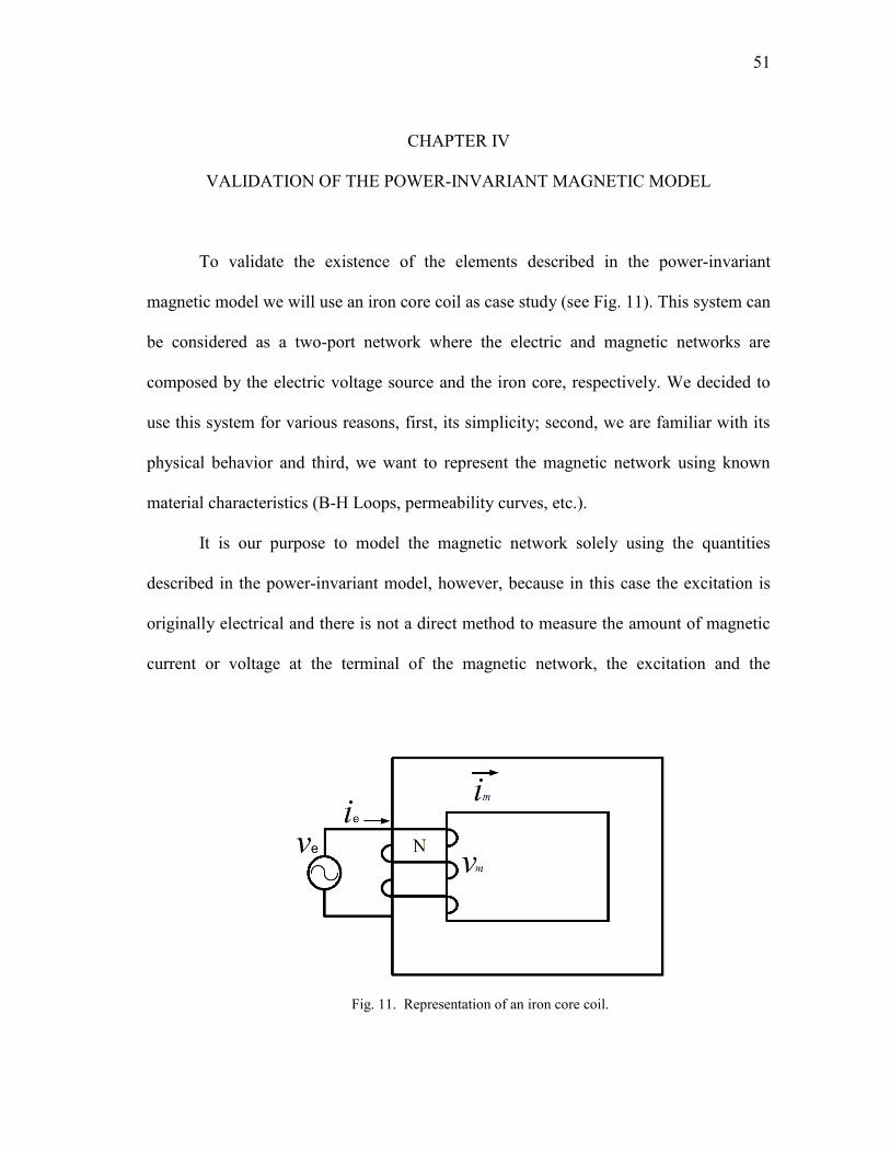
51

CHAPTER IV

VALIDATION OF THE POWER-INVARIANT MAGNETIC MODEL

To validate the existence of the elements described in the power-invariant

magnetic model we will use an iron core coil as case study (see Fig. 11). This system can

be considered as a two-port network where the electric and magnetic networks are

composed by the electric voltage source and the iron core, respectively. We decided to

use this system for various reasons, first, its simplicity; second, we are familiar with its

physical behavior and third, we want to represent the magnetic network using known

material characteristics (B-H Loops, permeability curves, etc.).

It is our purpose to model the magnetic network solely using the quantities

described in the power-invariant model, however, because in this case the excitation is

originally electrical and there is not a direct method to measure the amount of magnetic

current or voltage at the terminal of the magnetic network, the excitation and the

Fig. 11. Representation of an iron core coil.

52

response of the magnetic system have to be measured indirectly through the electric

terminal and then gyrated to the magnetic regime in order to analyze it.

A. Ideal Iron Core Coil Case Study

When the iron core coil presented in Fig. 11 is considered ideal, this is the copper

and iron losses are neglected, the easiest way to characterize the magnetic network is by

using the coil’s electric circuit model, shown in Fig. 12a. It is an electric voltage source

in series with an electric inductance and is mathematically expressed as,

[V] (87)

In this model, the iron core is depicted as a magnetic energy storage element by

the electric inductance. The element that performs this same function in the magnetic

regime is the magnetic capacitance. Therefore, we can model the ideal iron core coil as a

magnetic capacitance in series with a magnetic current source as it is shown in Fig. 12b.

According to gyrator theory, the electric voltage source can be modeled as a

magnetic current source of value

[Wb/s], (88)

Fig. 12. Representation of an ideal iron core coil a) electric circuit, b) magnetic circuit.

53

and the electric current is modeled as a magnetic voltage of value

[A]. (89)

Replacing (88) and (89) in (87),

[Wb/s]. (90)

This means that the value of the magnetic capacitance is equivalent to the electric

inductance and is expressed as,

[H]. (91)

This is consistent with gyrator theory [25] and with our expression of magnetic

capacitance because,

[H]. (92)

It is important to point out that even though this model does not represent either

the losses or hysteresis, it represents the linearity or nonlinearity of the material and can

be used to identify the saturation level of the material (see Fig. 13).

B. Real Iron Core Coil Case Study

The capacitance element alone does not represent the real behavior of an iron

core coil. Hysteresis and magnetic losses, among other factors, need to be taken into

consideration when modeling the magnetic network.

54

Such network or in this case the magnetic material can be characterized by

varying the excitation’s magnitude, frequency or waveform and analyzing how the

system responds to such variations. Hysteresis loops are good example of this technique.

These loops provide valuable information about the system under study, for

instance, hysteresis losses are represented by the area inside each loop and the saturation

level of the material can be identified using the tip of the major hysteresis loop. Also, the

shape of the loops is used to identify the type of magnetic the material. Fig. 14 shows the

hysteresis loops of a Grain-Oriented Electrical Steel material excited at 50 Hz where

each loop varies due to an amplitude variation. On the other hand, Fig. 15 shows the

hysteresis loops of the Magnetic Industries’ Permalloy 80 where each loop varies due to

a frequency variation.

According to our theory, in order to represent the real behavior of the magnetic

material we should model the network using the magnetic resistance, inductance and

capacitance. We understand that the effect of some of those elements is more significant

Fig. 13. Characteristic of a magnetic capacitance a) linear, b) nonlinear.

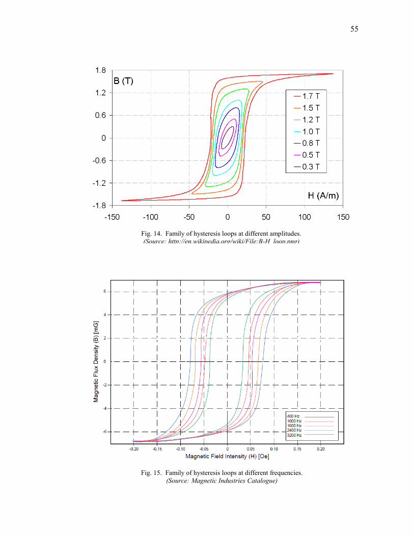
55

Fig. 14. Family of hysteresis loops at different amplitudes.

(Source: http://en.wikipedia.org/wiki/File:B-H_loop.png)

Fig. 15. Family of hysteresis loops at different frequencies.

(Source: Magnetic Industries Catalogue)

http://en.wikipedia.org/wiki/File:B-H_loop.png

56

than others in the model however, for completeness we will represent the network based

on the three elements. The reason behind this will be clarified in section 3.1.

Fig. 16 shows the eight possible configurations in which the elements could be

arranged. Each one of these configurations is a representation of the magnetic network

only. The elements can be either linear or nonlinear and the source can be either a

magnetic current or voltage source depending on the electric source.

1. Determining the Element’s Configuration based on Frequency Tests

In order to choose the correct configuration we need to perform a series of

conceptual tests. These tests are based on the response that the system shows due to

variation in magnitude and frequency of the excitation. In this case we will assume that

the system is excited with an electric current source of Ie value.

Rm

vm

im

Lm

Cm vm

imRm

Lm

Lm

Cm

vm

im RmCm

Cm

vm

im

Rm

Lm

vm

im Cm

RmLm Cm Rm

Lmvm

im

LmRm Cmvm

im

CmLm

Rmim

vm

Case No. 1 Case No. 2 Case No. 3 Case No. 4

Case No. 5 Case No. 6 Case No. 7 Case No. 8

Fig. 16. Magnetic network configurations.

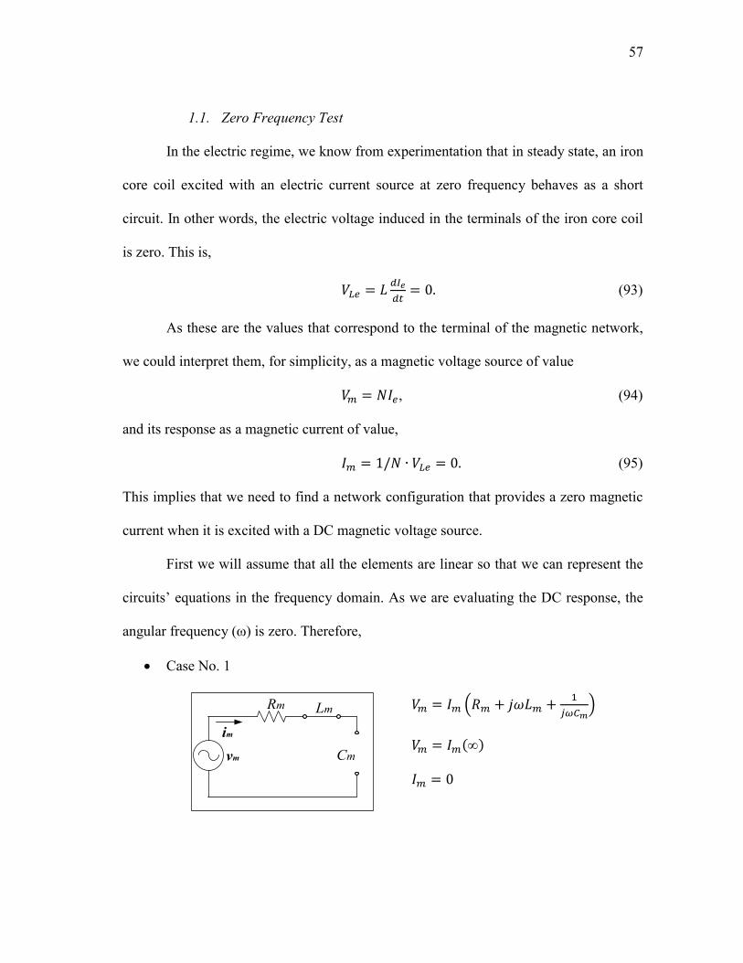
57

1.1. Zero Frequency Test

In the electric regime, we know from experimentation that in steady state, an iron

core coil excited with an electric current source at zero frequency behaves as a short

circuit. In other words, the electric voltage induced in the terminals of the iron core coil

is zero. This is,

(93)

As these are the values that correspond to the terminal of the magnetic network,

we could interpret them, for simplicity, as a magnetic voltage source of value

, (94)

and its response as a magnetic current of value,

(95)

This implies that we need to find a network configuration that provides a zero magnetic

current when it is excited with a DC magnetic voltage source.

First we will assume that all the elements are linear so that we can represent the

circuits’ equations in the frequency domain. As we are evaluating the DC response, the

angular frequency (ω) is zero. Therefore,

Case No. 1

Rm

vm

im

Lm

Cm

(

)

58

Case No. 2

vm

imRm

Lm

Cm

(

)

Case No. 3

vm

imRm

Cm

Lm

(

)

Case No. 4

Rm

Cm

Lm

vm

im

(

)

Case No. 5

vm

im Cm

Lm Rm

(

)

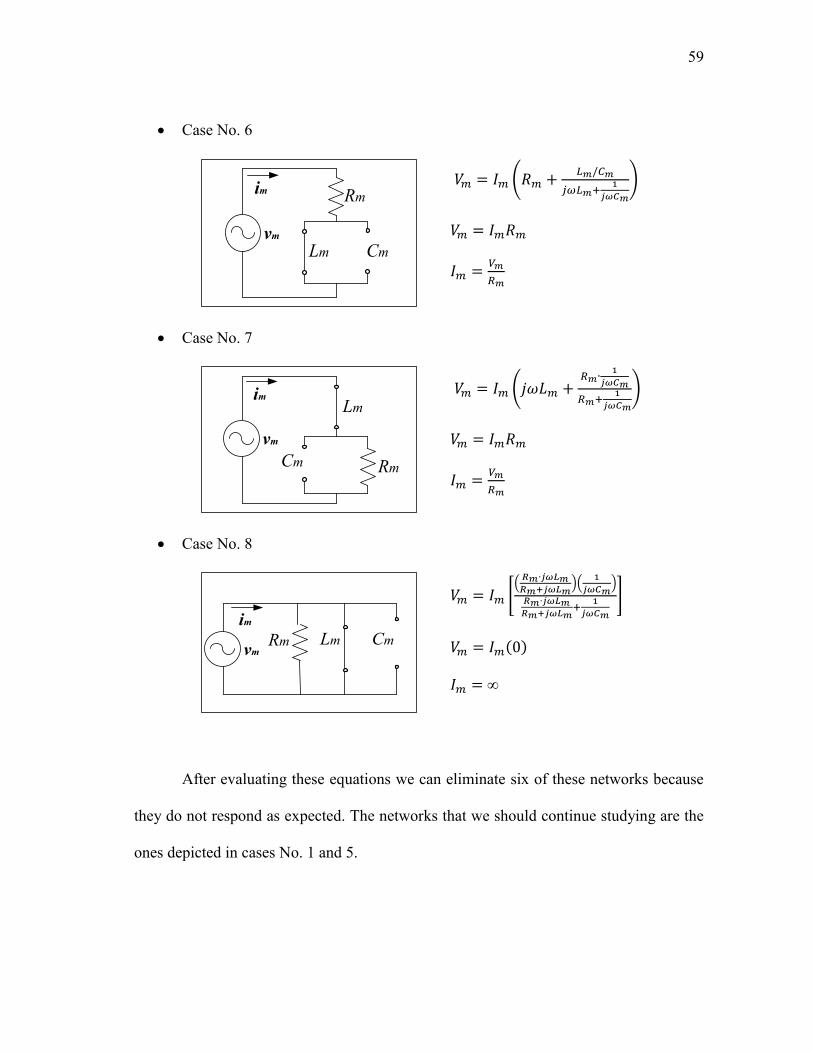
59

Case No. 6

vm

im

Cm

Rm

Lm

(

)

Case No. 7

vm

im

Rm

Lm

Cm

(

)

Case No. 8

Rm Lm Cmvm

im

*(

)(

)

+

After evaluating these equations we can eliminate six of these networks because

they do not respond as expected. The networks that we should continue studying are the

ones depicted in cases No. 1 and 5.

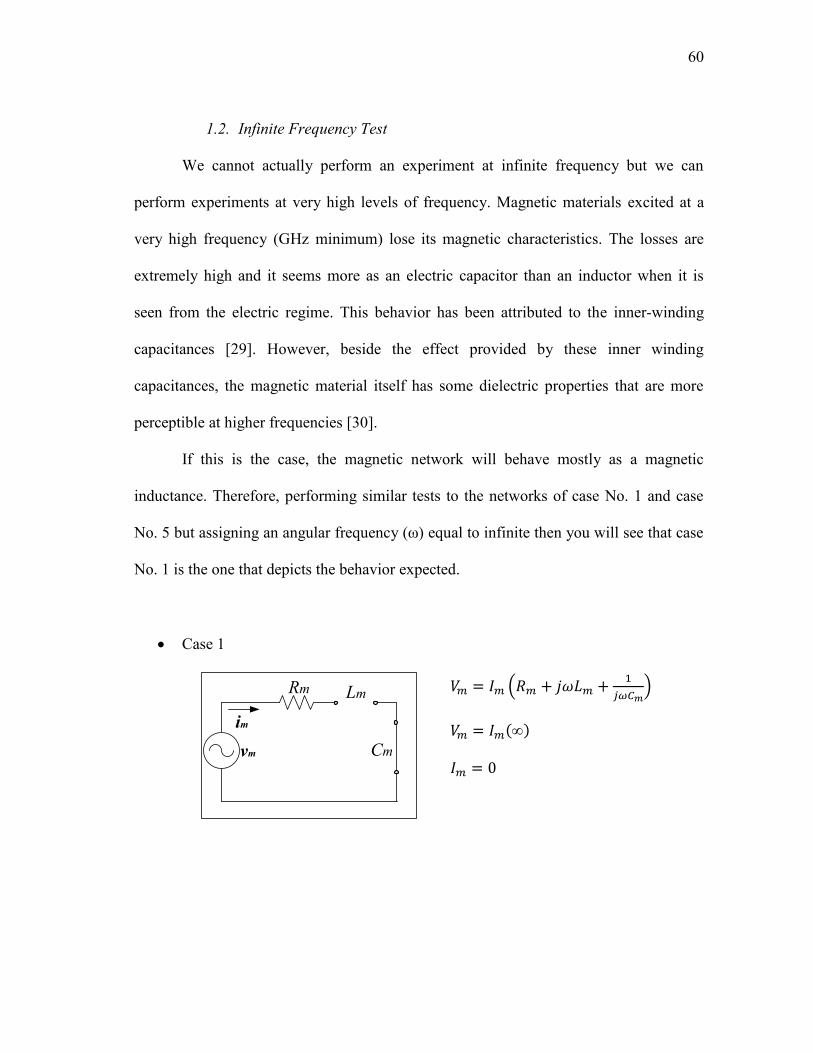
60

1.2. Infinite Frequency Test

We cannot actually perform an experiment at infinite frequency but we can

perform experiments at very high levels of frequency. Magnetic materials excited at a

very high frequency (GHz minimum) lose its magnetic characteristics. The losses are

extremely high and it seems more as an electric capacitor than an inductor when it is

seen from the electric regime. This behavior has been attributed to the inner-winding

capacitances [29]. However, beside the effect provided by these inner winding

capacitances, the magnetic material itself has some dielectric properties that are more

perceptible at higher frequencies [30].

If this is the case, the magnetic network will behave mostly as a magnetic

inductance. Therefore, performing similar tests to the networks of case No. 1 and case

No. 5 but assigning an angular frequency (ω) equal to infinite then you will see that case

No. 1 is the one that depicts the behavior expected.

Case 1

Rm

vm

im

Lm

Cm

(

)

61

Case 5

Rm

Cm

Lm

vm

im

(

)

1.3. Medium Frequency Test

Beside the fact that the network of case No. 1 provides the expected solution at

zero and infinite frequency, we need to verify that it models the magnetic material at the

levels of frequency most commonly used (Hz-MHz). At these frequencies, the dielectric

property of the magnetic material is very small and most of the times it is neglected.

Therefore, our network configuration should be able to represent the losses and the

energy storage capacity of the material.

If we perform a circuit analysis to the case No.1 and case No.5 neglecting the

inductance, the circuits need to be modified in order to represent that there is an almost

zero voltage drop at the terminals of the magnetic inductance or in other words, the

inductance is symbolized by a short circuit. Therefore,

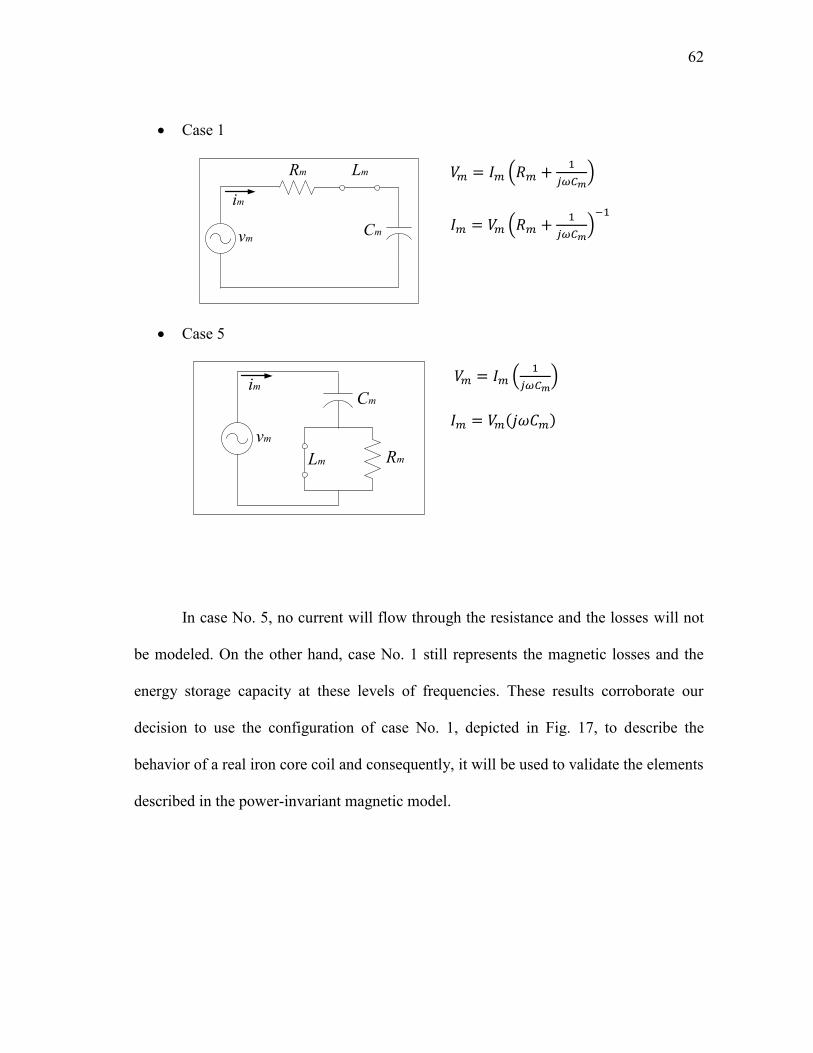
62

Case 1

LmRm

Cmvm

im

(

)

(

)

Case 5

vm

im

Lm Rm

Cm

(

)

In case No. 5, no current will flow through the resistance and the losses will not

be modeled. On the other hand, case No. 1 still represents the magnetic losses and the

energy storage capacity at these levels of frequencies. These results corroborate our

decision to use the configuration of case No. 1, depicted in Fig. 17, to describe the

behavior of a real iron core coil and consequently, it will be used to validate the elements

described in the power-invariant magnetic model.

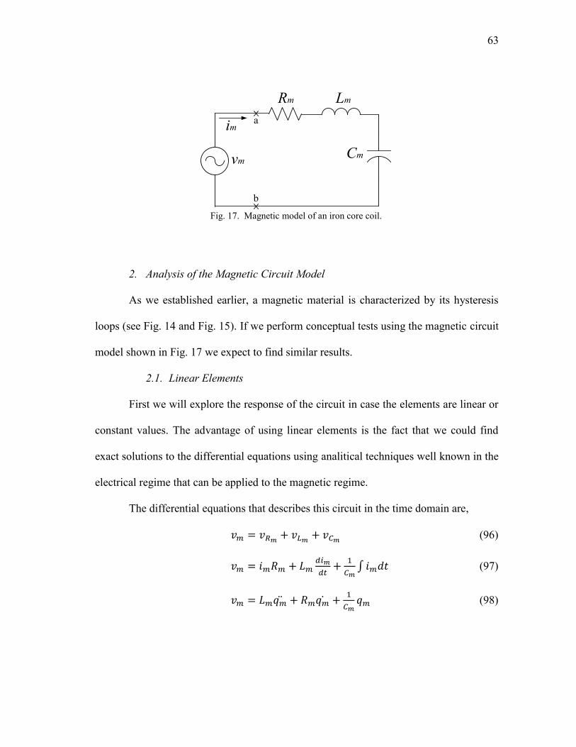
63

2. Analysis of the Magnetic Circuit Model

As we established earlier, a magnetic material is characterized by its hysteresis

loops (see Fig. 14 and Fig. 15). If we perform conceptual tests using the magnetic circuit

model shown in Fig. 17 we expect to find similar results.

2.1. Linear Elements

First we will explore the response of the circuit in case the elements are linear or

constant values. The advantage of using linear elements is the fact that we could find

exact solutions to the differential equations using analitical techniques well known in the

electrical regime that can be applied to the magnetic regime.

The differential equations that describes this circuit in the time domain are,

(96)

∫ (97)

(98)

LmRm

Cmvm

ima

b

Fig. 17. Magnetic model of an iron core coil.

64

The plot of the magnetic voltage at the terminals a-b versus the integral of the

magnetic current (qm) is proportional to the B-H hysteresis loop as,

[A/m], (99)

[T]. (100)

Table VII presents the values used to calculate the magnetic current of this

conceptual test. As the excitation of the system has a cosinusoidal waveform and the

elements are linear, the differential equations (97) and (98) can be solved easily in the

frequency domain instead that in the time domain using Laplace transformations or

phasors. The circuit’s current equation expressed using phasors is,

(

)

(101)

where the angular frequency .

The circuit’s equations in the time domain are,

[t·A], (102)

[Wb/s], (103)

TABLE VII

MAGNETIC PARAMETERS OF THE CONCEPTUAL TEST

Parameter Value Unit

Max. Magnetic Voltage 10.0 t·A

Magnetic Resistance 19.06 Ω-1

Magnetic Inductance 1.05e-9 F

Magnetic Capacitance 1.89e-5 H

Core’s Area 1.06 cm2

Core’s Length 10.1 cm

* The value of the core’s geometry has been based on the geometry of the toroidal core T157-34 of Micrometals, Inc.

65

[Wb]. (104)

Once we have obtained all the equations that describe the system we proceed to

find the family of hysteresis loops that result due to variations in amplitudes and

frequencies. Fig. 18 presents three hysteresis loops excited with voltage magnitudes of

2.5, 5 and 10 t·A at a frequency of 150 Hz. On the other hand, Fig. 19 presents a family

of hysteresis loops excited with a fixed magnetic voltage amplitude of 10 t·A but with

frequencies ranging from 50 Hz to 150 Hz. The magnetic field intensity and magnetic

flux density correspondent to the magnetic voltage and charge respectively, they are

calculated using (99) and (100).

-1.5

-1.0

-0.5

0

0.5

1.0

1.5

2.0

Ma

gn

etic F

lux D

en

sity (

B)

[T]

-100 100-80 80-60 -40 -20 0 20 40 60

Magnetic Field Intensity (H) [A/m]

Hmax = 24.75 A/m

Hmax = 49.50 A/m

Hmax = 99.00 A/m

Fig. 18. Family of hysteresis loops at different amplitudes (linear elements).

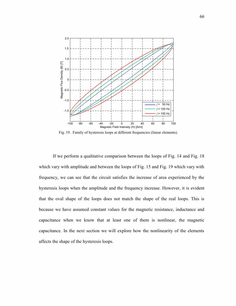
66

If we perform a qualitative comparison between the loops of Fig. 14 and Fig. 18

which vary with amplitude and between the loops of Fig. 15 and Fig. 19 which vary with

frequency, we can see that the circuit satisfies the increase of area experienced by the

hysteresis loops when the amplitude and the frequency increase. However, it is evident

that the oval shape of the loops does not match the shape of the real loops. This is

because we have assumed constant values for the magnetic resistance, inductance and

capacitance when we know that at least one of them is nonlinear, the magnetic

capacitance. In the next section we will explore how the nonlinearity of the elements

affects the shape of the hysteresis loops.

-1.5

-1.0

-0.5

0

0.5

1.0

1.5

2.0

Ma

gn

etic F

lux D

en

sity (

B)

[T]

-100 100-80 80-60 -40 -20 0 20 40 60

Magnetic Field Intensity (H) [A/m]

f = 50 Hz

f = 100 Hz

f = 150 Hz

Fig. 19. Family of hysteresis loops at different frequencies (linear elements).

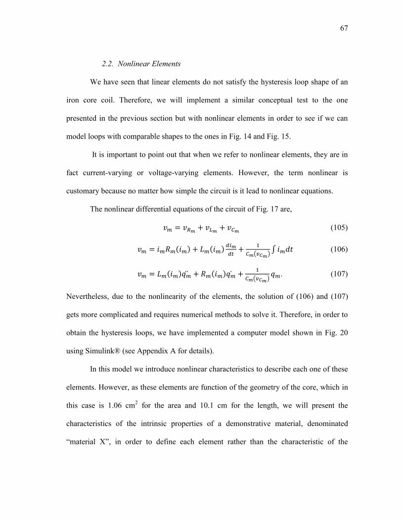
67

2.2. Nonlinear Elements

We have seen that linear elements do not satisfy the hysteresis loop shape of an

iron core coil. Therefore, we will implement a similar conceptual test to the one

presented in the previous section but with nonlinear elements in order to see if we can

model loops with comparable shapes to the ones in Fig. 14 and Fig. 15.

It is important to point out that when we refer to nonlinear elements, they are in

fact current-varying or voltage-varying elements. However, the term nonlinear is

customary because no matter how simple the circuit is it lead to nonlinear equations.

The nonlinear differential equations of the circuit of Fig. 17 are,

(105)

( )∫ (106)

( ) . (107)

Nevertheless, due to the nonlinearity of the elements, the solution of (106) and (107)

gets more complicated and requires numerical methods to solve it. Therefore, in order to

obtain the hysteresis loops, we have implemented a computer model shown in Fig. 20

using Simulink® (see Appendix A for details).

In this model we introduce nonlinear characteristics to describe each one of these

elements. However, as these elements are function of the geometry of the core, which in

this case is 1.06 cm2 for the area and 10.1 cm for the length, we will present the

characteristics of the intrinsic properties of a demonstrative material, denominated

“material X”, in order to define each element rather than the characteristic of the

68

elements itself; this is the permeability for the magnetic capacitance, the permittivity for

the magnetic inductance and the magnetic resistivity for the magnetic resistance. Fig. 21,

Fig. 22 and Fig. 23 show the aforementioned characteristics.

The hysteresis loops that we found using these characteristics are presented in

Fig. 24 for amplitudes of magnetic voltage ranging from 0.5 to 10 t·A and in Fig. 25 for

frequencies ranging from 10 Hz to 100 Hz. The curves at 500 Hz and 1 kHz were

calculated varying the magnetic resistivity curve as shown in Fig. 23. This was done in

order to simulate the increase in losses due to skin effect.

In order to calculate the magnetic current and charge, Simulink solves the

circuit’s ordinary differential equations by using the solver ODE45. This solver is based

on the Dormand-Prince numerical method which is a member of the Runge-Kutta family

Fig. 20. Simulink model using nonlinear elements.

http://en.wikipedia.org/wiki/Runge%E2%80%93Kutta

69

Fig. 21. Permeability’s nonlinear characteristic (µ=B/H).

Fig. 22. Permittivity’s nonlinear characteristic (ε=D/E).

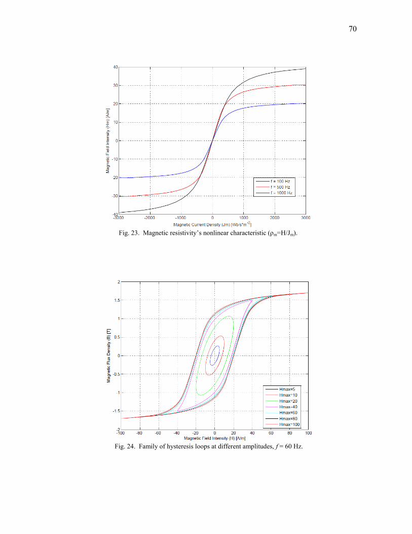
70

Fig. 23. Magnetic resistivity’s nonlinear characteristic (ρm=H/Jm).

Fig. 24. Family of hysteresis loops at different amplitudes, f = 60 Hz.

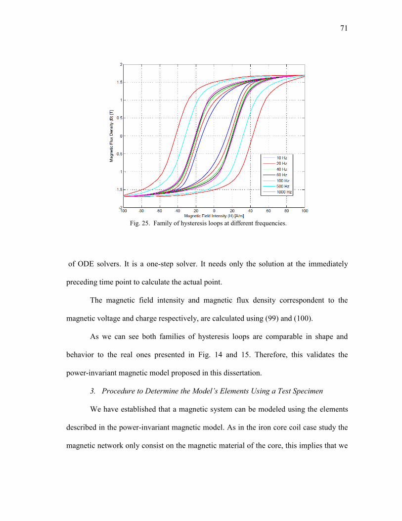
71

of ODE solvers. It is a one-step solver. It needs only the solution at the immediately

preceding time point to calculate the actual point.

The magnetic field intensity and magnetic flux density correspondent to the

magnetic voltage and charge respectively, are calculated using (99) and (100).

As we can see both families of hysteresis loops are comparable in shape and

behavior to the real ones presented in Fig. 14 and 15. Therefore, this validates the

power-invariant magnetic model proposed in this dissertation.

3. Procedure to Determine the Model’s Elements Using a Test Specimen

We have established that a magnetic system can be modeled using the elements

described in the power-invariant magnetic model. As in the iron core coil case study the

magnetic network only consist on the magnetic material of the core, this implies that we

Fig. 25. Family of hysteresis loops at different frequencies.

72

can characterize the material based on these elements and consequently, on their intrinsic

properties. In this section we will present the techniques that we have developed in order

to find each one of these properties.

3.1. Fundamentals of the Test

It has been well established in electric circuits that depending on the value of the

system’s impedance, the amplitude and phase of the response vary. The same rule

applies for magnetic systems and it can be demonstrated if we perform a series of simple

waveform analysis using linear elements. The insights obtained from this analysis will

be applied to find the characteristics of each element.

Resistance Case

First, we will use a magnetic system where the impedance is only a magnetic

resistance. If the system is excited with a voltage source , then

the response is given by,

, (108)

. (109)

If we plot the magnetic voltage and currents as shown in Fig. 26, we can see that

for a given magnetic voltage the amplitude of the current varies according to the value of

the magnetic resistance. Furthermore, the phase angle of the current remains in phase

with the phase angle of the voltage. This means that the maximum value of the voltage

waveform corresponds to the maximum value of the current waveform.

73

To emulate the hysteresis loop we plot the instantaneous magnetic voltage versus

the instantaneous magnetic charge, as shown in Fig. 27. This plot is a loop with certain

area because the magnetic charge is phase shifted 90° with respect to the voltage. Also,

we can see that no matter the variation of the resistance the direction of the loop remains

parallel to the horizontal axis.

Inductance Case

In this case we will present a magnetic system where the impedance is only a

magnetic inductance. The expression of the current if is,

∫ , (110)

, (111)

Fig. 26. Magnetic voltage at 60 Hz and currents for different values of resistance.

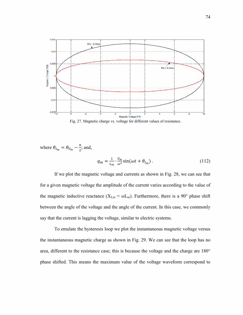
74

where

; and,

. (112)



the magnetic inductive reactance (XLm = ωLm). Furthermore, there is a 90° phase shift

between the angle of the voltage and the angle of the current. In this case, we commonly

say that the current is lagging the voltage, similar to electric systems.


the instantaneous magnetic charge as shown in Fig. 29. We can see that the loop has no

area, different to the resistance case; this is because the voltage and the charge are 180°

phase shifted. This means the maximum value of the voltage waveform correspond to

Fig. 27. Magnetic charge vs. voltage for different values of resistance.

75

the minimum value of the charge waveform. Also, no matter the variation of the

inductance the direction of the loop remains being a line with a negative slope.

Fig. 29. Magnetic charge vs. voltage for different values of inductance.

Fig. 28. Magnetic voltage at 60 Hz and currents for different values of inductance.

76

Capacitance Case

In this case we will present a magnetic system where the impedance is only a

magnetic capacitance. The expression of the response if is,

, (113)

, (114)

, (115)

where

; and,

. (116)



Fig. 30. Magnetic voltage at 60 Hz and currents for different values of capacitance.

77

the magnetic capacitive reactance (XCm = (ωCm)-1

). Furthermore, there is a 90° phase

shift between the angle of the voltage and the angle of the current. In this case, we

commonly say that the current is leading the voltage, similar to electric systems.


the instantaneous magnetic charge as shown in Fig. 31. We can see that the loop has no

area, as in the inductance case, this is because the voltage and the charge are in phase.

This means that the maximum value of the voltage waveform correspond to the

maximum value of the charge waveform. Also, no matter the variation of the capacitance

the direction of the loop remains being a line with a positive slope.

Series Rm, Lm and Cm Case

In this case we will present a magnetic system where the impedance has the

configuration of the three elements in series. This is the configuration we are using to

represent the iron core coil (see Fig. 17).

Fig. 31. Magnetic charge vs. voltage for different values of capacitance.

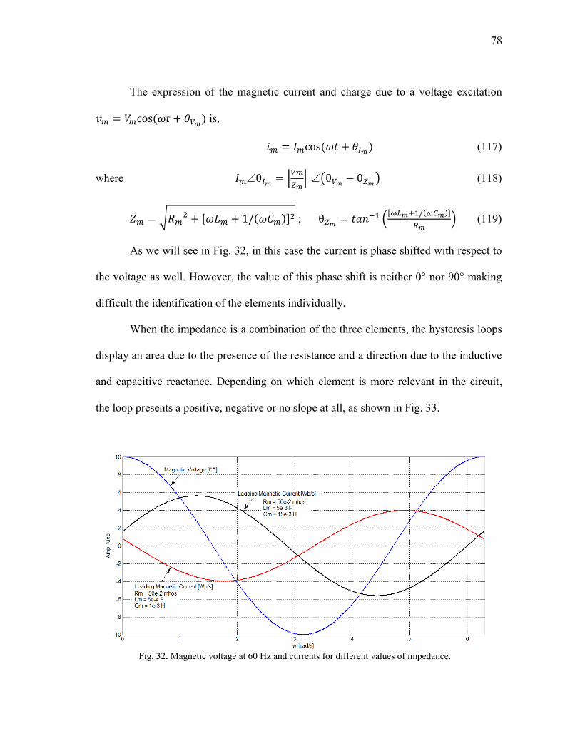
78

The expression of the magnetic current and charge due to a voltage excitation

is,

(117)

where |

| (

) (118)

√ [ ] ;

([ ]

) (119)

As we will see in Fig. 32, in this case the current is phase shifted with respect to

the voltage as well. However, the value of this phase shift is neither 0° nor 90° making

difficult the identification of the elements individually.

When the impedance is a combination of the three elements, the hysteresis loops

display an area due to the presence of the resistance and a direction due to the inductive

and capacitive reactance. Depending on which element is more relevant in the circuit,

the loop presents a positive, negative or no slope at all, as shown in Fig. 33.

Fig. 32. Magnetic voltage at 60 Hz and currents for different values of impedance.

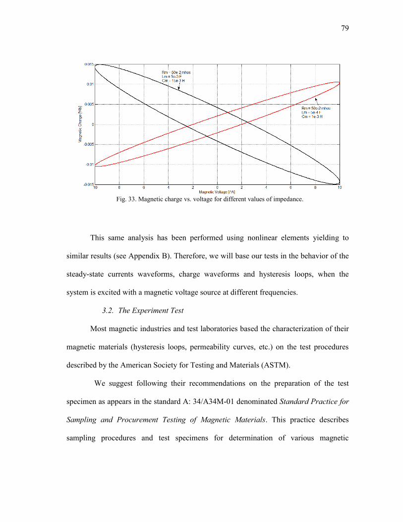
79

This same analysis has been performed using nonlinear elements yielding to

similar results (see Appendix B). Therefore, we will base our tests in the behavior of the

steady-state currents waveforms, charge waveforms and hysteresis loops, when the

system is excited with a magnetic voltage source at different frequencies.

3.2. The Experiment Test

Most magnetic industries and test laboratories based the characterization of their

magnetic materials (hysteresis loops, permeability curves, etc.) on the test procedures

described by the American Society for Testing and Materials (ASTM).

We suggest following their recommendations on the preparation of the test

specimen as appears in the standard A: 34/A34M-01 denominated Standard Practice for

Sampling and Procurement Testing of Magnetic Materials. This practice describes

sampling procedures and test specimens for determination of various magnetic

Fig. 33. Magnetic charge vs. voltage for different values of impedance.

80

properties of both soft and hard magnetic materials [31]. However, we suggest using the

schematic shown in Fig. 34 to build the apparatus of this experiment.

The system is excited with an AC current source. The oscilloscope will be used

to capture instantaneous value of the electric current and voltage induced at the electric

terminals of the core as these values are manipulated in order to find the hysteresis loops

that characterize the magnetic material.

The procedures developed to find the parameters of the magnetic model are

based on the family of hysteresis loops at different frequencies and amplitudes.

However, as those loops are product of the manipulation of the measured electric current

and voltage, these waveforms can be used as well. They are gyrated into the magnetic

regime and directly used as terminal values of the magnetic model of Fig. 17.

At this point, we have designed and presented a general description of the

Fig. 34. Schematic illustration of the test apparatus.

81

experiment settings. However, in order to avoid measurement inaccuracies we decided to

use published conventional data, this is manufacturer’s hysteresis loops, instead of

performing our own experimentation. Unfortunately, the data that we obtained to

characterize a magnetic material was insufficient. Nevertheless, as our objective is to

explain the procedures developed to find the magnetic elements, we decided to avoid the

experiments complications and use the hysteresis loops that result from the computer

model that we developed in Simulink as we already show that this model generates

hysteresis loops with similar behavior to the real ones.

3.3. The Conceptual Test

In this conceptual test we will perform the same tests we would have

implemented in the experiment test. As we will use the model developed in Simulink,

depicted in Fig. 20, we expect to find the same material characteristics that we

introduced to proof the functionality of the model in the first place. However, because

we want to emulate the experiment test, we will only use the waveforms of the magnetic

circuit terminals in order to find the elements’ characteristics. This is done because these

magnetic current and voltage are a representation of the electric voltage and current that

we would have measured using the oscilloscope.

3.3.1. Quasi-static Frequency Test

The first test that we will implement is exciting the model at the lowest none zero

frequency possible. In other words, we have to run the model at a quasi-static mode. If

the system is excited with a zero frequency magnetic voltage, the steady state magnetic

current will be zero as explained in the zero-frequency test. However, we need to

82

analyze the phase angle, amplitude and shape of the steady state response and the quasi-

static frequency allows us to do that.

Fig. 35 shows the waveform of the magnetic voltage and current at steady state.

The voltage applied is a cosinusoisal waveform at 0.5 Hz with an amplitude equal to 10

t·A. It is evident that the magnetic current is leading the voltage exactly 90°; this implies

that under this quasi-static condition the magnetic capacitance is the element that

predominates in the circuit.

In Appendix C we present magnetic current waveforms for different amplitudes

of magnetic voltage, you will see that regarding the nonlinearity of the magnetic current,

the phase angle remains almost 90° shifted. This implies that we can characterize the

nonlinearity of the magnetic capacitance following this method.

Fig. 35. Magnetic voltage and current at 0.5 Hz.

83

The capacitance equation (120) expresses a point by point relation between the

magnetic flux or magnetic charge (φ, qm) and the magnetic voltage (vm). Therefore, the

characteristic of the magnetic capacitance can be found by plotting the magnetic charge

versus the magnetic voltage at a low frequency.

(120)

Fig. 36 displays a family of hysteresis loops, each one result of an increase in

amplitude of the magnetic voltage. As (120) is a point by point relation, we expected

loops with zero area but instead these plots present loops with very small area as result.

This happens because another element is starting to affect the response. In order to

reduce the area of the loops the frequency of operation should be lower. However, if the

value of this area is very small, the capacitance characteristic can be approximated by a

line connecting the tips of each loop as shown in Fig. 36.

It is known that the characteristic of the magnetic capacitance depends on the

geometry of the specimen therefore, it is better to provide a more general description of

this element in terms of its intrinsic property, the permeability. Fig. 37 presents the

circuit’s hysteresis loops but in terms of the field intensities. The permeability is the

point by point relation between the magnetic flux density and the magnetic field

intensity. It can also be displayed as shown in Fig. 38, where the left and right side of the

curve represent the saturation of the material and the line at the tip of the curve

represents the state at which the capacitance behaves as a linear element.

84

Fig. 36. Magnetic capacitance characteristic (Family of hysteresis loops at 0.5 Hz).

Fig. 37. Permeability characteristic (Family of hysteresis loops at 0.5 Hz).

85

3.3.2. Medium Frequency Test

The second test that we will implement is exciting the model at a medium

frequency. Fig. 39 shows the waveform of the input magnetic voltage and current at

steady state. The voltage applied is a cosinusoisal waveform at 60 Hz with an amplitude

equal to 10 t·A. In this case it is not so evident the phase shift between the magnetic

current and voltage. This implies that under this condition, more than one element

affects the response of the circuit. In Appendix C we present magnetic current

waveforms for different amplitudes of magnetic voltage. The nonlinearity of the

elements is reflected in the current as the amplitude of the magnetic voltage increases.

As we already obtained the characteristic of the capacitance we can calculate the

magnetic voltage of this capacitance. From “measurement” we have the instantaneous

magnetic current of the circuit and consequently the magnetic charge of the capacitance.

Fig. 38. Permeability vs. magnetic field intensity.

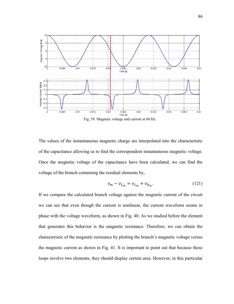
86

The values of the instantaneous magnetic charge are interpolated into the characteristic

of the capacitance allowing us to find the correspondent instantaneous magnetic voltage.

Once the magnetic voltage of the capacitance have been calculated, we can find the

voltage of the branch containing the residual elements by,

. (121)

If we compare the calculated branch voltage against the magnetic current of the circuit

we can see that even though the current is nonlinear, the current waveform seems in

phase with the voltage waveform, as shown in Fig. 40. As we studied before the element

that generates this behavior is the magnetic resistance. Therefore, we can obtain the

characteristic of the magnetic resistance by plotting the branch’s magnetic voltage versus

the magnetic current as shown in Fig. 41. It is important to point out that because these

loops involve two elements, they should display certain area. However, in this particular

Fig. 39. Magnetic voltage and current at 60 Hz.

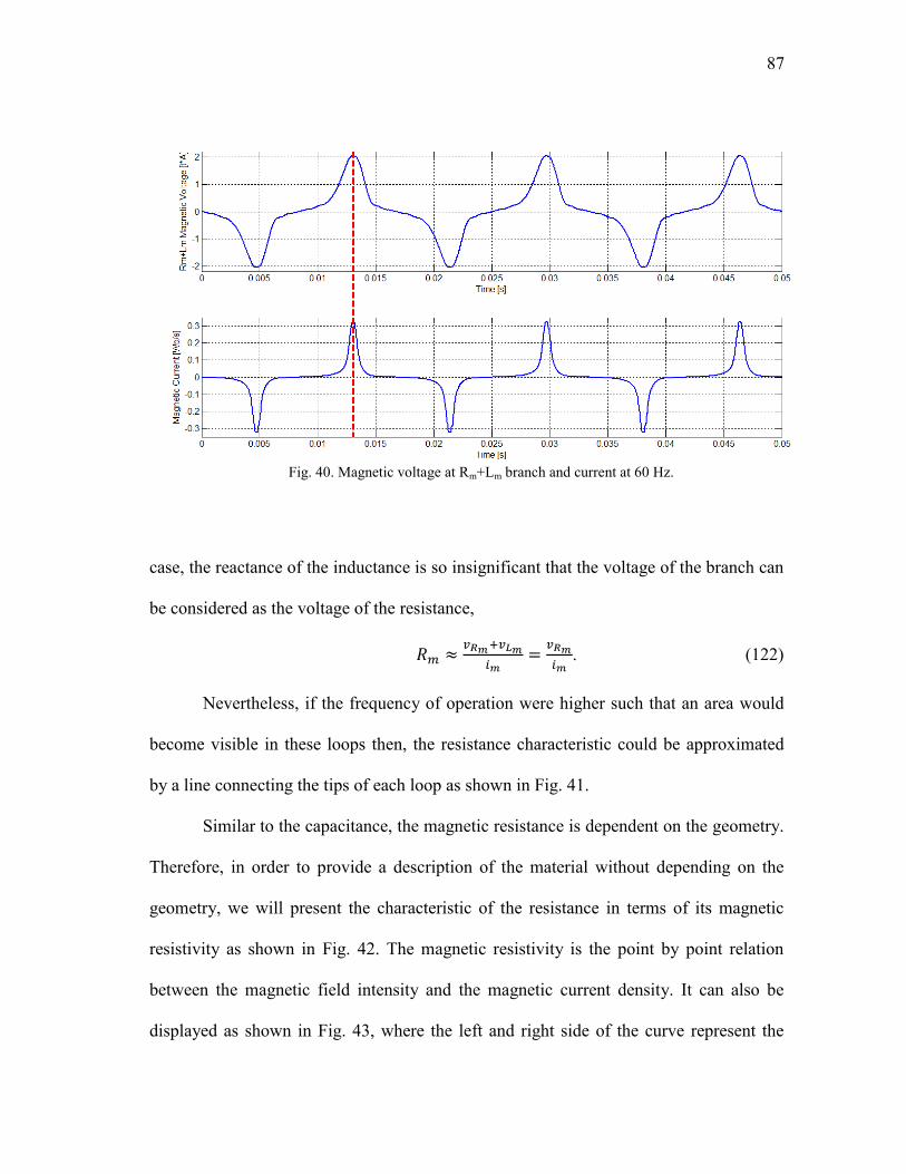
87

case, the reactance of the inductance is so insignificant that the voltage of the branch can

be considered as the voltage of the resistance,

. (122)

Nevertheless, if the frequency of operation were higher such that an area would

become visible in these loops then, the resistance characteristic could be approximated

by a line connecting the tips of each loop as shown in Fig. 41.

Similar to the capacitance, the magnetic resistance is dependent on the geometry.

Therefore, in order to provide a description of the material without depending on the

geometry, we will present the characteristic of the resistance in terms of its magnetic

resistivity as shown in Fig. 42. The magnetic resistivity is the point by point relation

between the magnetic field intensity and the magnetic current density. It can also be

displayed as shown in Fig. 43, where the left and right side of the curve represent the

Fig. 40. Magnetic voltage at Rm+Lm branch and current at 60 Hz.

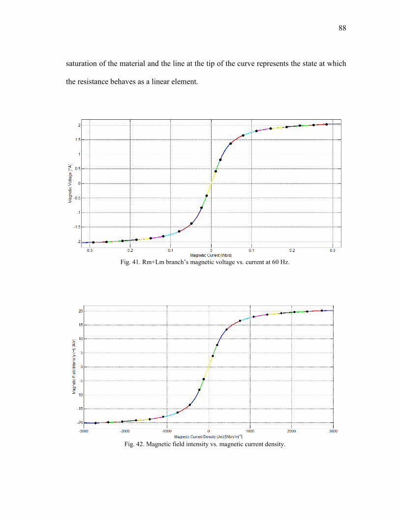
88

saturation of the material and the line at the tip of the curve represents the state at which

the resistance behaves as a linear element.

Fig. 42. Magnetic field intensity vs. magnetic current density.

Fig. 41. Rm+Lm branch’s magnetic voltage vs. current at 60 Hz.

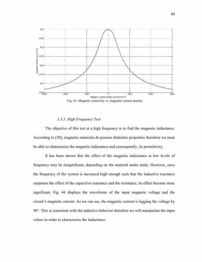
89

3.3.3. High Frequency Test

The objective of this test at a high frequency is to find the magnetic inductance.

According to [30], magnetic materials do possess dielectric properties therefore we must

be able to characterize the magnetic inductance and consequently, its permittivity.

It has been shown that the effect of the magnetic inductance at low levels of

frequency may be insignificant, depending on the material under study. However, once

the frequency of the system is increased high enough such that the inductive reactance

surpasses the effect of the capacitive reactance and the resistance, its effect become more

significant. Fig. 44 displays the waveforms of the input magnetic voltage and the

circuit’s magnetic current. As we can see, the magnetic current is lagging the voltage by

90°. This is consistent with the inductive behavior therefore we will manipulate the input

values in order to characterize the inductance.

Fig. 43. Magnetic resistivity vs. magnetic current density.

90

Equation (123) expresses that the magnetic inductance is a point by point relation

between the electric charge and the magnetic current therefore if we plot this variables

we can find the inductance characteristic as shown in Fig. 45.

Fig. 44. Magnetic voltage and current at 1 GHz.

Fig. 45. Electric charge vs. magnetic current at 1 GHz.

91

(123)

In this particular case, the frequency applied is of a value such that no area is

seen inside the loop. However if the loop would have shown a small area, it will mean

that another element is affecting the response of the system and an approximation similar

to the one that we applied to the magnetic capacitance would have been needed. This is,

generating a family of loops at different amplitudes and connecting the tips of the loops.

Fig. 46 and Fig. 47 display the characteristic of the permittivity.

Fig. 46. Electric flux density vs. electric field intensity at 1 GHz.

92

Fig. 47. Permittivity vs. electric field intensity at 1 GHz.

93

CHAPTER V

APPLICATION OF THE POWER-INVARIANT MAGNETIC MODEL

Designing electromagnetic devices is not an easy task. There are many variables

that need to be taken into consideration, even compromised, in order to achieve a

satisfactory design. Commonly, the designer must make tradeoffs among size,

efficiency, weight, price and type of materials before landing a suitable final design.

Along the years, engineers have used various approaches in order to reach this goal. We

believe that the power-invariant magnetic model is a good candidate as a first approach

design tool.

Furthermore, the similarities between the electric and the power-invariant

magnetic model enlighten us to introduce analysis techniques, well understood in

electric systems but novel in the magnetic ones. These techniques will allow us to

perform power transfer analysis in the magnetic regime as well.

In order to demonstrate the capabilities of the power-invariant magnetic model

we will design and perform steady-state analysis in a novel concept that we have

denominated magnetic transmission line.

The idea of a magnetic transmission line was born after comparing the model of

a short electric transmission line against our model of the transformer (see Fig. 48),

which is an extension of the iron core coil model presented in the previous chapter. The

objective of this study is to explore the feasibility of using a magnetic material instead of

the conventional electric conductor to transport power.

94

ie,p

ve,p

imag

ie,s

+

-

ve,s

+

-

imag

Np Ns

Np Ns

MTL

iel

ETL

+

-

+

-

vs vL

a) Schematic of a transformer/MTL

b) Model of a magnetic transmission line

c) Model of an electric transmission line

Fig. 48. Comparison of the model of a magnetic transmission line

and an electric transmission line.

95

A. Designing a Magnetic Transmission Line

The design of a magnetic transmission line, similar to the design of an electric

transmission line includes,

the material of the conductor,

the size, weight and cost of the conductor,

the power loss and temperature rise,

the frequency of operation,

efficiency of the system, among others.

The power-invariant magnetic model can be used to design a magnetic

transmission line because it includes most of the aforementioned factors. The advantage

of this model is that it does not need families of hysteresis loops to model the behavior

of the magnetic material. This model characterizes the material based on its intrinsic

properties (permeability, permittivity and magnetic resistivity). Therefore, it is easier to

find the geometry, frequency, etc., that provides the optimal design for a given condition

of operation. However, it is important to point out that this model is still in its first stage

of development, therefore some effects like copper losses, eddy current losses, fringing

flux and the temperature dependence of the magnetic material, have not been included

yet.

In this section we will design a magnetic transmission line using the material’s

properties described in the previous chapter. Simultaneously, we will perform a power

transfer analysis using a Matlab®-based code that we have developed in order to solve

the systems’ nonlinear differential equations.

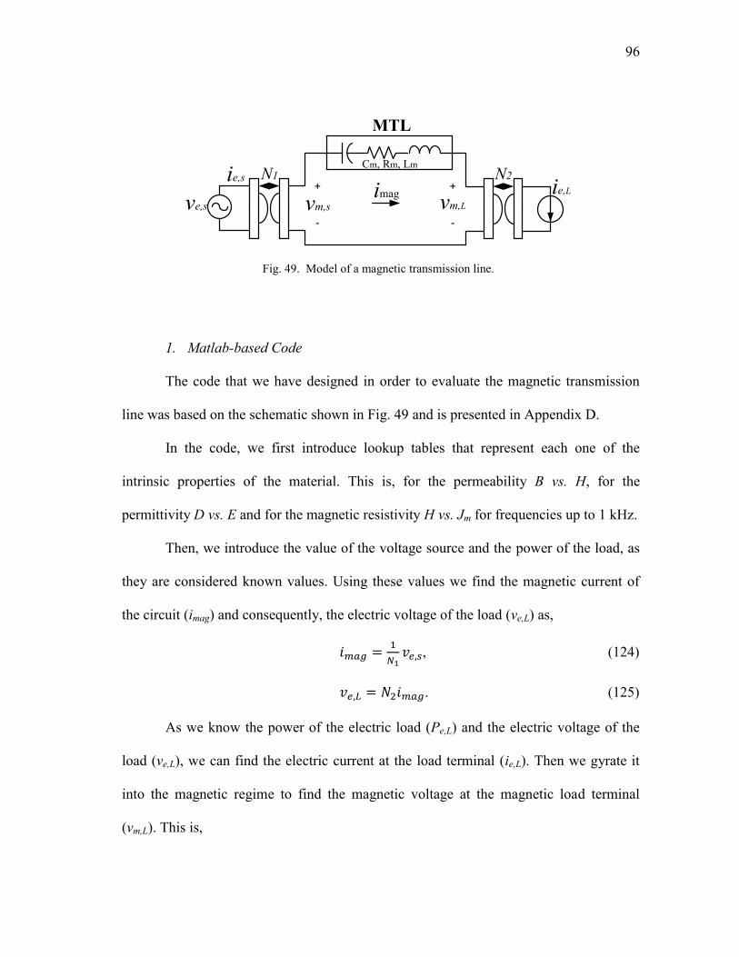
96

1. Matlab-based Code

The code that we have designed in order to evaluate the magnetic transmission

line was based on the schematic shown in Fig. 49 and is presented in Appendix D.

In the code, we first introduce lookup tables that represent each one of the

intrinsic properties of the material. This is, for the permeability B vs. H, for the

permittivity D vs. E and for the magnetic resistivity H vs. Jm for frequencies up to 1 kHz.

Then, we introduce the value of the voltage source and the power of the load, as

they are considered known values. Using these values we find the magnetic current of

the circuit (imag) and consequently, the electric voltage of the load (ve,L) as,

, (124)

. (125)

As we know the power of the electric load (Pe,L) and the electric voltage of the

load (ve,L), we can find the electric current at the load terminal (ie,L). Then we gyrate it

into the magnetic regime to find the magnetic voltage at the magnetic load terminal

(vm,L). This is,

imag

N1 N2

MTL

Cm, Rm, Lm

ie,s

vm,s vm,L

+

-

+

-

ve,s

ie,L

Fig. 49. Model of a magnetic transmission line.

97

. (126)

As the voltage drop of the magnetic transmission line depends on the

characteristics of each element and these elements depend on the geometry of the

specimen, we create two loops. The external loop iterates values of area while the inner

loop iterates values of length. These values are introduced into the permeability,

permittivity and magnetic resistivity tables in order to find the characteristic of the

capacitance (qmag vs. vcmag), the inductance (qelec vs. imag) and the magnetic resistance

(vrmag vs. imag), respectively.

The voltage drop (vmtl) is calculated adding the voltage of each one of the

elements. In order to do so, the instantaneous values of the magnetic current (imag) are

interpolated inside these elements characteristics. The result will give the resistance’s

magnetic voltage and the inductance’s electric charge. This electric charge is

differentiated in order to find the inductance’s magnetic voltage. Similarly, we

interpolate the instantaneous values of the integral of the magnetic current inside the

capacitance characteristic in order to find the capacitance’s voltage.

After the voltage drop of the magnetic transmission line is calculated, we can

find the magnetic voltage at the terminal source (vm,s) adding the magnetic voltage at the

terminal load and the line’s voltage drop. This magnetic voltage is gyrated into the

electric regime in order to find the electric current of the source,

. (127)

After the voltages and currents of the system are calculated, we can evaluate the

performance of the system using three factors, the losses which is the power dissipated

98

as heat, the efficiency which is a measure of the amount power transferred from the

source to the load and the power factor, which is a measure of the capacity of the line to

transmit power. Therefore, we include its calculations in the code as well.

The power dissipated by the magnetic resistance is the average of the

instantaneous power at the resistance. This is,

∑ ( ) . (128)

Because the model is power-invariant, the efficiency of the magnetic line (η) can

be calculated using the net power at either the electric or magnetic regime terminals. The

efficiency is given by,

. (129)

Due to the nonlinearity of the system, we recommend to calculate the net power from the

instantaneous power equation as,

∑ ( ) ∑ ( )

, (130)

and

∑ ( ) ∑ ( )

. (131)

The power factor is the ratio of the power that does work (net power) versus the

total power injected into the system (apparent power). As the model is power-invariant

the power factor can be calculated either at the electric or magnetic source terminal. It is

calculated using,

. (132)

99

The apparent power is calculated using the root mean square (RMS) values of the

voltage and current waveforms. In the general case, the RMS value of a waveform can

be calculated using,

√∑

. (133)

Then, the apparent power is calculated based on,

. (134)

The calculation of the power factor using this method is consistent with the

calculation of the power factor using the distortion factor and the displacement factor of

the current waveform used in power electronics [32].

2. Case Study

We will design a magnetic transmission line whose source (Ve,s = 200 Vpk) and

load (Pe,L = 1 kW) are in the electric regime as presented in Fig. 49. We will evaluate

how changes in length, area, frequency of operation and number of turns affect the

efficiency of the system.

Fig. 50 and Fig. 51 show the efficiency vs. core length profile of a system that is

excited at 60 Hz and 1 kHz, respectively. In both cases, the primary and secondary

windings (N1, N2) have a value of 500 turns.

In these figures, each curve represents a different core’s area. The minimum

practical area (Fig. 50, Ac,min = 6 cm2 and Fig. 51, Ac,min = 36 mm

2 ) depends on the

amplitude of the magnetic charge (qm) and the maximum flux level of the material that

we want to apply, in this case, the saturation level.

100

Fig. 50. Efficiency vs. core length for various areas (system at 60 Hz).

Fig. 51. Efficiency vs. core length for various areas (system at 1 kHz).

101

The amplitude of the magnetic charge depends on the amplitude of the magnetic

current and the frequency of operation. If the amplitude of the magnetic current is fixed

and the frequency increases, then the amplitude of the magnetic charge will decrease.

Therefore, in order to maintain the maximum flux density, the area has to be reduced as

well. This is given by,

, (135)

, (136)

where,

. (137)

And as we know,

. (138)

Therefore,

⁄ . (139)

Below this value, the waveform of the magnetic voltage of the line and consequently, the

electric current at the source becomes much distorted due to the nonlinearities of the

line’s capacitive element and it might be unpractical to use.

The advantage of increasing the frequency is that we can transfer power using a

magnetic conductor of a small core area. Nevertheless, it also has the disadvantage of

increasing the losses and therefore, reducing the efficiency of the system.

Another important factor that needs to be taken into consideration, when

designing a magnetic line, is the amount of distortion that the waveform of the electric

current is allowed to experience. For instance, Fig. 52 and 53 show the electric current

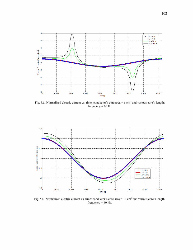
102

Fig. 52. Normalized electric current vs. time; conductor’s core area = 6 cm2 and various core’s length;

frequency = 60 Hz

.


frequency = 60 Hz.

103

waveforms of a magnetic line at 60 Hz, for different core lengths with a core area of 6

cm2 and 12 cm

2, respectively. The amplitude of these currents has been normalized with

respect to the amplitude of the source current as if the line were ideal (depicted as blue

dotted line). This is, the electric current at the source is equal to the electric current at the

load.

Analyzing these figures we can see that increasing the area of the core reduces

the distortion of the electric current. This happens because the magnetic flux density is

reduced and the magnetic transmission line operates near the linear region of the

magnetic capacitance characteristic.

The same situation is seen in Fig. 54 and 55 which show the electric current

waveforms of a magnetic line at 1 kHz, for different core lengths with a core area of 36

mm2 and 2 cm

2, respectively. The amplitude of these currents has been normalized with

respect to the amplitude of the source current similar to the previous frequency.

As the distortion of the electric current is dependent on the nonlinearity of the

elements of the magnetic transmission line, the power factor is a measure of the

distortion of the electric current and consequently, it describes the capacity of the

magnetic line to transmit power. Table VIII, presents the power factor of the system

which currents are presented in Fig. 52 – Fig. 55.

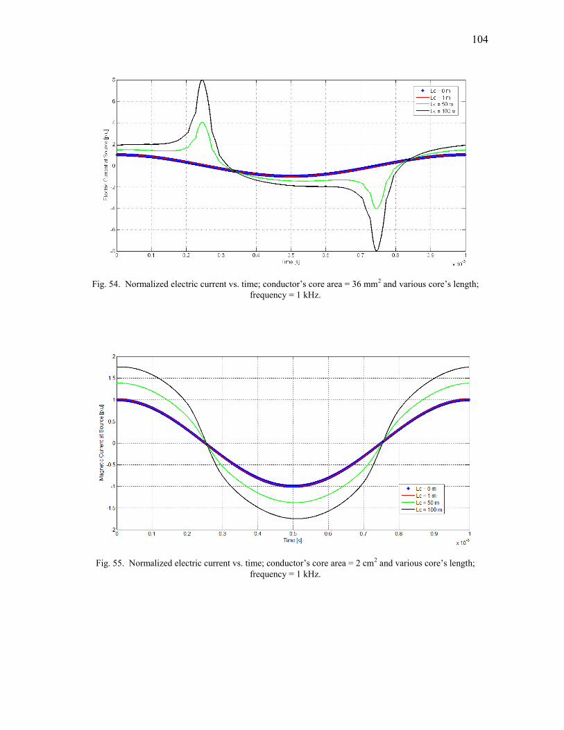
104

Fig. 54. Normalized electric current vs. time; conductor’s core area = 36 mm2 and various core’s length;

frequency = 1 kHz.


frequency = 1 kHz.

105

After evaluating the efficiency, the waveform of the input electric current and the

power factor of the system we can choose a geometry and frequency of operation for our

magnetic transmission line. This is,

Frequency of operation = 1 kHz

Core’s length = 25 m

Core’s area = 36 mm2

This geometry, using 500 turns in the primary and secondary windings, yield to

an efficiency of 78.77% and a power factor of 0.84. If we want to increase the efficiency

of the system, we can do so by increasing the number of turns of the windings. This

tactic improves the efficiency because an increase in the number of turns reduces the

magnetic current, consequently reducing the magnetic losses. We understand that

increasing the number of turns increases the electric copper losses however these losses

are out of the scope of this analysis. If we tripled the number of turns in both windings,

the efficiency rises to 92.5% and the power factor improves to 0.99. This means that the

reactive effect of the line is almost imperceptible.

TABLE VIII

POWER FACTOR DUE TO DIFFERENT FREQUENCIES AND GEOMETRIES

Core’s Length

[m]

f = 60 Hz f = 1 kHz

Ac = 6 cm2 Ac = 12 cm2 Ac = 36 mm2 Ac = 2 cm2

0 1.00 1.00 1.00 1.00

1 0.99 1.00 0.99 1.00

50 0.58 0.99 0.68 0.99

100 0.38 0.98 0.54 0.99

106

The electric current at the source side is presented in Fig. 56. The magnetic

current and voltages waveform of the magnetic transmission line are presented in Fig. 57

and Fig. 58.

It is important to point out that even though in this case we have chosen a design

where the magnetic transmission line possess the same frequency that the rest of the

system, we have to evaluate the possibility of using power electronics at the electric

source and load side of the magnetic transmission line in order to manipulate the

magnetic excitation of the line to seek maximum power transfer.

Fig. 56. Electric current (ie,s) vs. time.

107

Fig. 58. Magnetic voltages vs. time.

Fig. 57. Magnetic current (imag) vs. time.

108

2.1. Comparison between a Magnetic and an Electric Conductor

If we compare the area of the magnetic conductor used in this case study to

transmit 1 kW of power, Ac,m = 36 mm2, with an electric conductor used to transmit the

same amount of power at 60 Hz. This is an AWG 14 wire with an ampacity up to 20 A

and an area, Ac,e = 2 mm2. The magnetic conductor is 18 times bigger than its electric

counterpart.

The electric resistance of an AWG 14 wire of 25 m length is approximately

207.15 mΩ. This will result in copper losses of approximately 10.4 watts which will

yield to an efficiency of 98.97%. If we compare this value to the efficiency of the

magnetic transmission line system, 92.5%, this implies that transmitting power through

an electric media is 1.07 times better than doing so in the magnetic regime.

Even though this comparison suggests that is better to transmit power in the

electric regime rather than in the magnetic regime, we believe that the importance of this

study lies in the fact that we have established the possibility of transferring power using

a magnetic media and also, we have supplied the tools to design and analyze this type of

system.

109

CHAPTER VI

SUMMARY AND FUTURE RESEARCH

In this chapter we present the summary of the work accomplished during the

course of this research. Also, we establish the contributions of this work and provide

some recommendations for future research in this area of study.

A. Summary

In this dissertation, we have presented a model for magnetic systems that is

standard with other regimes models, for instance, electric, mechanic and hydraulic

systems. This model has been based on the principle of conservation of energy and

consists in describing the energy transfer process in terms of the effort, flow and three

elements that describe how the energy is dissipated or stored during the energy transfer

process. We have defined these terms for the magnetic regime and used them to model a

simple magnetic system, an iron core coil.

As in the iron core coil case study, the process occurs solely in the magnetic

material we represented it as a magnetic network composed of three elements, magnetic

resistance, capacitance and inductance. However, due to the geometry dependence of

these elements and aiming to give a general description of the material, we decided to

better describe the magnetic material in terms of the elements’ intrinsic properties,

magnetic resistivity, permeability and permittivity. Therefore, we have developed and

presented a methodology based on a conceptual experiment in order to find the

aforementioned material’s intrinsic properties.

110

In order to analyze the iron core coil, we developed analytical and numerical

techniques that solved the network’s differential equations. Also, we presented the

equations used to calculate the power dissipated and the energy stored in the material.

Finally, after evaluating the analysis techniques that this model offers to the

modeling of magnetic systems and observing the similarities that it has compared to the

electric model, we explored the possibility of transmitting power through the magnetic

media using a magnetic transmission line analogue to transmitting power using an

electric transmission line.

In Chapter I we addressed the importance of magnetic materials in modern

technologies and described how researches in manufacturing and modeling techniques

have improved during the years. We presented a series of numerical techniques currently

used to model different systems and gave reasons that support why the use of lumped

parameters is still a valid option. Also, in this chapter we described three magnetic

models that use lumped parameters, these are, the reluctance model, the permeance-

capacitor model and the gyrator capacitor model. Finally, we established the problem

that we want to solve with this work, the research objectives and the organization of the

dissertation.

In Chapter II we included a literature review of electromagnetic theory in order

to show the close relation that exists between the electric and magnetic regimes. Also,

we presented a description of the different types of magnetic materials, with an especial

interest in the properties of ferromagnetic materials as they are the most common

magnetic material used in modern applications.

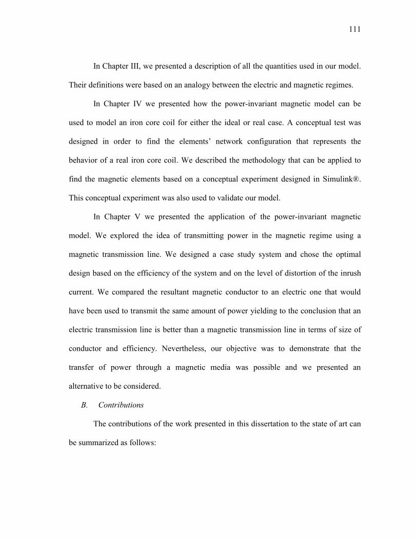
111

In Chapter III, we presented a description of all the quantities used in our model.

Their definitions were based on an analogy between the electric and magnetic regimes.

In Chapter IV we presented how the power-invariant magnetic model can be

used to model an iron core coil for either the ideal or real case. A conceptual test was

designed in order to find the elements’ network configuration that represents the

behavior of a real iron core coil. We described the methodology that can be applied to

find the magnetic elements based on a conceptual experiment designed in Simulink®.

This conceptual experiment was also used to validate our model.

In Chapter V we presented the application of the power-invariant magnetic

model. We explored the idea of transmitting power in the magnetic regime using a

magnetic transmission line. We designed a case study system and chose the optimal

design based on the efficiency of the system and on the level of distortion of the inrush

current. We compared the resultant magnetic conductor to an electric one that would

have been used to transmit the same amount of power yielding to the conclusion that an

electric transmission line is better than a magnetic transmission line in terms of size of

conductor and efficiency. Nevertheless, our objective was to demonstrate that the

transfer of power through a magnetic media was possible and we presented an

alternative to be considered.

B. Contributions

The contributions of the work presented in this dissertation to the state of art can

be summarized as follows:

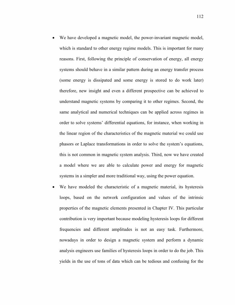
112

We have developed a magnetic model, the power-invariant magnetic model,

which is standard to other energy regime models. This is important for many

reasons. First, following the principle of conservation of energy, all energy

systems should behave in a similar pattern during an energy transfer process

(some energy is dissipated and some energy is stored to do work later)

therefore, new insight and even a different prospective can be achieved to

understand magnetic systems by comparing it to other regimes. Second, the

same analytical and numerical techniques can be applied across regimes in

order to solve systems’ differential equations, for instance, when working in

the linear region of the characteristics of the magnetic material we could use

phasors or Laplace transformations in order to solve the system’s equations,

this is not common in magnetic system analysis. Third, now we have created

a model where we are able to calculate power and energy for magnetic

systems in a simpler and more traditional way, using the power equation.

We have modeled the characteristic of a magnetic material, its hysteresis

loops, based on the network configuration and values of the intrinsic

properties of the magnetic elements presented in Chapter IV. This particular

contribution is very important because modeling hysteresis loops for different

frequencies and different amplitudes is not an easy task. Furthermore,

nowadays in order to design a magnetic system and perform a dynamic

analysis engineers use families of hysteresis loops in order to do the job. This

yields in the use of tons of data which can be tedious and confusing for the

113

engineer and time consuming even when processing the data using a

computer. Our approach seeks to reduce the amount of data that we have to

manipulate when modeling a magnetic material.

We presented a basic case study where we analyzed the feasibility of using

the magnetic material as a power transfer media. It has been called magnetic

transmission line analogous to an electric transmission line and it is an

innovative concept because to our knowledge, the magnetic media has not

been used specifically for this purpose. It provides an alternative to transfer

power in cases where the electric media might not be safe to use or where the

magnetic material provides a more efficient transfer of power than the

electric one.

C. Future Research

After culminating the research presented in this dissertation, we have identified

numerous lines of work related to this topic, for instance:

Identify the magnetic resistivity, permeability and permittivity of different

magnetic materials. In order to do so, we will need to design a test bench

where we could recreate the methodology proposed in this dissertation.

Include the effect of flux leakage, fringing flux and air gaps into the model’s

network configuration, in order to provide an even more realistic model to

magnetic systems.

Use the power-invariant magnetic model to model other more complex

magnetic systems, for instance, solenoids, transformers, motors, etc.,

114

Expand the use of this model from lumped parameters to a distributed model

based on lumped parameters, similar to the magnetic equivalent circuit

(MEC) model [33]. The difference lies in the fact that current MEC models

use the reluctance as base element, in our case, we will need to include the

three magnetic elements. However, we will need to explore the advantages

and disadvantages of expanding the lumped model into a distributed model.

Keep exploring the feasibility of using the magnetic transmission line to

transport power, evaluating the possibility of developing a complete power

system in the magnetic regime. This is using magnetic sources and loads.

115

REFERENCES

[1] R. C. O’Handley, “Modern Magnetic Materials: Principles and Applications,” 1st

ed., New York: John Wiley & Sons Inc., 2000, ch.1: Introduction and Overview,

pp. 1-22.

[2] J. M. D. Coey, “Magnetism and Magnetic Materials,” 1st ed., United Kingdom:

Cambridge University Press, 2009, ch.1: Introduction, pp. 13.

[3] A. Iványi, “Hysteresis Models in Electromagnetic Computation,” 1st ed.,

Budapest: Akadémiai Kiadó, 1997, ch1: Introduction, pp. 1-3.

[4] K. H. J. Buschow and F. R. De Boer, “Physics of Magnetism and Magnetic

Materials,” 2nd

ed., New York: Kluwer Academic Publishers, 2004, ch.1:

Introduction, pp. 1.

[5] S. S. Rao, “The Finite Element Method in Engineering,” 1st ed., Burlington, MA:

Elsevier Butterworth-Heinemann, 2005, ch.1: Overview of Finite Element

Method, pp. 7.

[6] Members of the Staff of the Department of Electrical Engineering at the

Massachusetts Institute of Technology, “Electric Circuits: A First Course in

Circuit Analysis for Electrical Engineers,” 1st ed. vol.1, New York: John Wiley

& Sons, 1943, pp.125-128.

[7] S. J. Chapman, “Máquinas Eléctricas,” 3rd

ed. vol.1, Colombia, Bogotá: McGraw

Hill, 2000, ch.1: Introducción a los Principios de Máquinas, pp. 8-29.

[8] R. W. Buntenbach, “Analogs between magnetic and electrical circuits,”

Electronic Products, vol. 12, pp. 108-113, Oct. 1969.

[9] D. C. Hamill, “Gyrator-capacitor modeling: a better way of understanding

magnetic components,” in Proc. 9th Annu. Applied Power Electronics and

Conference and Exposition, Florida: Orlando, 1994, vol.1, pp. 326-332.

[10] D. C. Hamill, “Lumped equivalent circuits of magnetic components: the gyrator-

capacitor approach,” IEEE Trans. Power Electron., vol. 8, no. 2, pp. 97-103,

Apr. 1993.

[11] V. P. Popov, “The Principles of Theory of Circuits,” Russia, Moscow: Higher

School, 1845, pp. 496. Available:

http://en.wikipedia.org/wiki/Magnetic_inductance.

116

[12] V. P. Popov, “The Principles of Theory of Circuits,” Russia, Moscow: Higher

School, 1845, pp. 496. Available:

http://en.wikipedia.org/wiki/Magnetic_effective_resistance.

[13] B. D. H. Tellegen, “The gyrator, a new electric network element,” Philips Res.

Rep., vol. 3, pp. 81-101, Apr. 1948.

[14] R. Y. Barazarte, G. G. González, and M. Ehsani, “Generalized Gyrator Theory,”

IEEE Trans. Power Electron., vol. 25, no. 7, pp. 1832-1837, July 2010.

[15] P. Davies, “The Forces of Nature,” 2nd

ed., United Kingdom: Cambridge

University Press, 1986, Available:

http://en.wikipedia.org/wiki/Fundamental_interaction.

[16] G. W. Carter, “The Electromagnetic Field in its Engineering Aspects,” 2nd

ed.,

New York: American Elsevier Publishing Company, 1967, ch.2: The Electric

Field of Charges in Free Space, pp. 5, 6.

[17] B. D. Cullity and C. D. Graham, “Introduction to Magnetic Materials,” 1st ed.,

New Jersey: John Wiley & Sons, Inc., 2009, ch.1: Definition and Units, pp. 1-22.

[18] N. A. Spaldin, “Magnetic Materials: Fundamentals and Applications,” 2nd

ed.,

New York: Cambridge University Press, 2011, ch.1: Review of Basic

Magnetostatics, pp. 3-12.

[19] D. Voltmer, “Fundamental of Electromagnetics 1: Internal Behavior of Lumped

Elements,” 1st ed., San Rafael, CA: Morgan & Claypool,” 2007, ch.2: Capacitors,

pp. 91-130.

[20] G. Bertotti, “Hysteresis in Magnetism,” 1st ed., San Diego, CA: Academic Press,

1998, ch.1: Introduction, pp. 3-20.

[21] L. Néel, “Propriétées Magnétiques des Ferrites; Férrimagnétisme et

antiferromagnétisme,” Annales de Physic (Paris), vol. 3, pp. 137-198, 1948.

Available in English: http://en.wikipedia.org/wiki/Ferrimagnetism.

[22] G. W. Carter, “The Electromagnetic Field in its Engineering Aspects,” 2nd

ed.,

New York: American Elsevier Publishing Company, 1967, ch.7: The Magnetic

Effect of Iron, pp. 128.

[23] Members of the Staff of the Department of Electrical Engineering at the

Massachusetts Institute of Technology, “Magnetic Circuits and Transformers: A

http://en.wikipedia.org/wiki/Ferrimagnetism

117

First Course for Power and Communication Engineers,” 2nd

ed. vol.2, New York:

John Wiley & Sons, 1956, ch.5: Losses in Magnetic Cores Containing Time-

Varying Fluxes, pp.124-134.

[24] F. T. Brown, “Engineering System Dynamics: A Unified Graph-Centered

Approach,” 2nd

ed., Boca Raton, FL: CRC Press, 2007, ch.1: Introduction, pp. 1-

16.

[25] S. E. Gay, “Modeling of Motor Drive Dynamics by Generalized Impedance

Converter Theory,” Master Thesis, Department of Electrical and Computer

Engineering, Texas A&M University, College Station, TX, 2001.

[26] M. Zahn, “Electromagnetic Field Theory: A Problem Solving Approach,” 1st ed.,

New York: John Wiley & Sons, 1979, ch.3: Polarization and Conduction, pp.

135-151.

[27] S. S. Attwood, “Electric and Magnetic Fields,” 3rd

ed., New York: John Wiley &

Sons, 1956, ch.4: Electric Current, pp. 116-118.

[28] H. H. Woodson and J. R. Melcher, “Electromechanical Dynamics Part I: Discrete

Systems,” 1st ed., New York: John Wiley & Sons, 1968, ch.2: Lumped

Electromechanical Elements, pp. 76.

[29] A. Massarini and M. K. Kazimierczuk, “Self-Capacitance of Inductors,” IEEE

Trans. Power Electron., vol. 12, no. 4, pp. 671–676, July 1997.

[30] M. W. Hyde IV and M. J. Havrilla, “A nondestructive technique for determining

complex permittivity and permeability of magnetic sheet materials using two

flanged rectangular waveguides,” PIER., vol. 79, pp. 367–686, 2008.

[31] ASTM International, “Standard Practice for Sampling and Procurement Testing

of Magnetic Materials,” Annual Book of ASTM Standards, West Conshohocken,

PA: ASTM International, vol. 03.04, pp. 1-4, 2006.

[32] Cool Power Solutions Library, Nurmijärvi, Finland: Cool Power Solutions, ch.4:

Power Factor Correction, pp. 4. Available:

http://www.coolpowersolutions.fi/Eng/library.htm

[33] B. Sheikh-Ghalavand, S. Vaez-Zadeh, and A. H. Isfahani, “An improved

magnetic equivalent circuit model for iron-core linear permanent-magnet

synchronous motors,” IEEE Trans. Magnetics, vol. 46, no. 1, pp. 112-120,

January 2010.

118

APPENDIX A

IRON-CORE COIL MODEL

This appendix presents in detail, the model for the iron-core coil developed in

Simulink. We programmed our own numerical tool that solves the system’s nonlinear

differential equations in case the user does not possess Simulink. This code is Matlab-

based and is designed to solve the system’s differential equations for either a current or

voltage excitation. Both programs give the same steady-state results. Therefore, in order

to prove it, we compare the system’s magnetic current, charge and voltages of the

elements of both methods.

A. Simulink’s model

As shown in Fig. A.1, this model mainly consists of the voltage source and three

Fig. A.1. Simulink model using nonlinear elements.

119

subsystems that represent the nonlinear capacitance, resistance and inductance. It also

contains voltage and current measurements.

Fig. A.2, Fig. A.3 and Fig. A.4 presents the capacitance, resistance and

inductance subsystems, respectively.

Fig. A.2. Magnetic capacitance subsystem.

Fig. A.3. Magnetic resistance subsystem.

120

B. Matlab-based Code

Fig. A.5 presents the block diagram of the code. As you can see, we first

Fig. A.5. Matlab-based code block diagram.

Fig. A.4. Magnetic inductance subsystem.

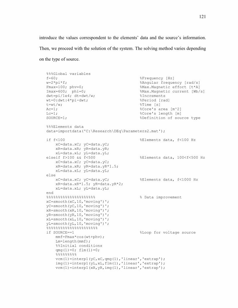
121

introduce the values correspondent to the elements’ data and the source’s information.

Then, we proceed with the solution of the system. The solving method varies depending

on the type of source.

%%%Global variables

f=60; %Frequency [Hz]

w=2*pi*f; %Angular frequency [rad/s]

Fmax=100; phv=0; %Max.Magnetic effort [t*A]

Imax=600; phi=0; %Max.Magnetic current [Wb/s]

dwt=pi/1e4; dt=dwt/w; %Increments

wt=0:dwt:4*pi-dwt; %Period [rad]

t=wt/w; %Time [s]

Ac=1; %Core's area [m^2]

Lc=1; %Core's length [m]

SOURCE=1; %Definition of source type

%%%Elements data

data=importdata('C:\Research\DEq\Parameters2.mat');

if f<100 %Elements data, f<100 Hz

xC=data.xC; yC=data.yC;

xR=data.xR; yR=data.yR;

xL=data.xL; yL=data.yL;

elseif f>100 && f<500 %Elements data, 100<f<500 Hz

xC=data.xC; yC=data.yC;

xR=data.xR; yR=data.yR*1.5;


else

xC=data.xC; yC=data.yC; %Elements data, f<1000 Hz

xR=data.xR*1.5; yR=data.yR*2;


end

%%%%%%%%%%%%%%%%%%%%% % Data improvement

xC=smooth(xC,10,'moving')';

yC=smooth(yC,10,'moving')';

xR=smooth(xR,10,'moving')';

yR=smooth(yR,10,'moving')';

xL=smooth(xL,10,'moving')';

yL=smooth(yL,10,'moving')';

%%%%%%%%%%%%%%%%%%%%%%

if SOURCE==1 %Loop for voltage source

mmf=Fmax*cos(wt+phv);

Lm=length(mmf);

%%Initial conditions

qmg(1)=0; flm(1)=0;

%%%%%%%%%

vcm(1)=interp1(yC,xC,qmg(1),'linear','extrap');

img(1)=interp1(yL,xL,flm(1),'linear','extrap');

vrm(1)=interp1(xR,yR,img(1),'linear','extrap');

122

vlm(1)=mmf(1)-vcm(1)-vrm(1);

for k=2:1:Lm

flm(k)=vlm(k-1)*dt+flm(k-1);

img(k)=interp1(yL,xL,flm(k),'linear','extrap');

qmg(k)=img(k)*dt+qmg(k-1);

vcm(k)=interp1(yC,xC,qmg(k),'linear','extrap');

vrm(k)=interp1(xR,yR,img(k),'linear','extrap');

vlm(k)=mmf(k)-vcm(k)-vrm(k);

end

elseif SOURCE==2 %Loop for current source

img=Imax*cos(wt+phi);

Lm=length(img);

%%Initial conditions

qmg(1)=0;

vcm(1)=interp1(yC,xC,qmg(1),'linear','extrap');

vrm(1)=interp1(xR,yR,img(1),'linear','extrap');

flm(1)=interp1(xL,yL,img(1),'linear','extrap');

flm(2)=interp1(xL,yL,img(2),'linear','extrap');

vlm(1)=(flm(2)-flm(1))/dt;

mmf(1)=vcm(1)+vrm(1)+vlm(1);

%%%%%%%%%

for k=2:1:Lm-1

qmg(k)=img(k-1)*dt+qmg(k-1);

vcm(k)=interp1(yC,xC,qmg(k),'linear','extrap');

vrm(k)=interp1(xR,yR,img(k),'linear','extrap');

flm(k+1)=interp1(xL,yL,img(k+1),'linear','extrap');

vlm(k)=(flm(k+1)-flm(k))/dt;

mmf(k)=vcm(k)+vrm(k)+vlm(k);

end

qmg(Lm)=qmg(2); flm(Lm)=flm(2); mmf(Lm)=mmf(2);

vcm(Lm)=vcm(2); vrm(Lm)=vrm(2); vlm(Lm)=vlm(2);

end

clc

Note: We need to point out that the solution of the system during the current source loop will diverge if the

initial value of current produces a charge above the saturation level specified by the capacitance

characteristic. In order to solve this, the user can modify the value of the current or the geometry of the

system until the charge reaches the limits mentioned.

C. Comparison of Simulink’s and our Matlab-based code system response.

This comparison was made assuming that the system has a cosinusoidal magnetic

voltage source of 100 Vpk at 60 Hz. The elements have the nonlinear intrinsic properties

shown in Fig. 21, 22 and 23 and the geometry of the core is unitary. This is Ac = 1 m2

and Lc = 1 m.

123

Fig. A.6. Magnetic current.vs. time.

Fig. A.7. Magnetic charge vs. time.

124

Fig. A.8. Resistance’s magnetic voltage vs. time.

Fig. A.9. Capacitance’s magnetic voltage vs. time.

125

Fig. A.11. Inductance’s electric charge vs. time.

Fig. A.10. Inductance’s magnetic voltage vs. time.

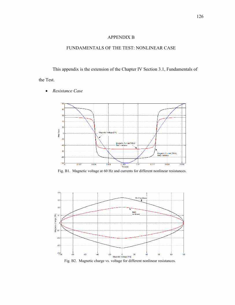
126

APPENDIX B

FUNDAMENTALS OF THE TEST: NONLINEAR CASE

This appendix is the extension of the Chapter IV Section 3.1, Fundamentals of

the Test.

Resistance Case

Fig. B2. Magnetic charge vs. voltage for different nonlinear resistances.

Fig. B1. Magnetic voltage at 60 Hz and currents for different nonlinear resistances.

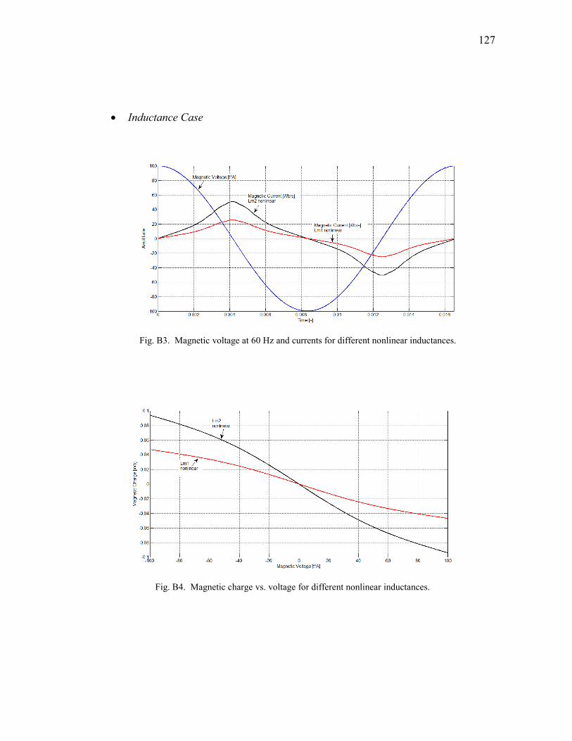
127

Inductance Case

Fig. B4. Magnetic charge vs. voltage for different nonlinear inductances.

Fig. B3. Magnetic voltage at 60 Hz and currents for different nonlinear inductances.

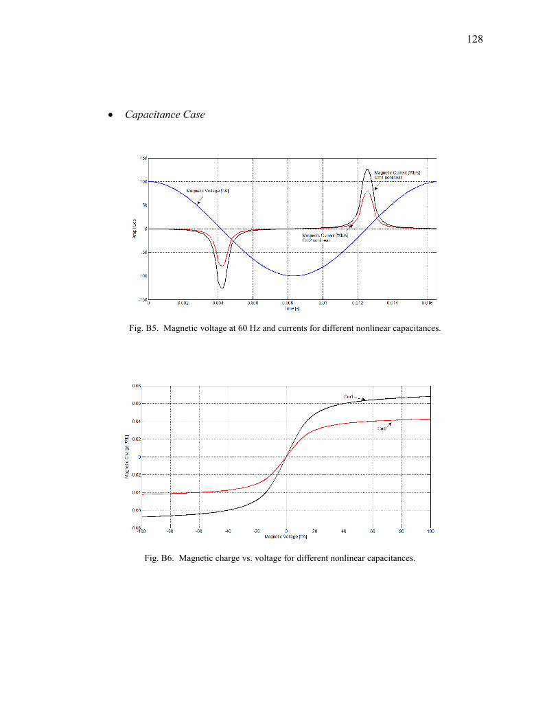
128

Capacitance Case

Fig. B6. Magnetic charge vs. voltage for different nonlinear capacitances.

Fig. B5. Magnetic voltage at 60 Hz and currents for different nonlinear capacitances.

129

APPENDIX C

MAGNETIC VOLTAGES AND CURRENTS

This appendix is an extension of Chapter IV. Section 3.3 and contains the plots

of magnetic voltages vs. time and current vs. time when the system is excited at different

frequencies. The objective is to demonstrate that the nonlinearity does not affect the

phase shift of the element, it only affects the waveform.

Case 1: Frequency = 0.5 Hz

Fig. C.1. Magnetic voltage and current at 0.5 Hz for a voltage amplitude of 0.5 A·t.

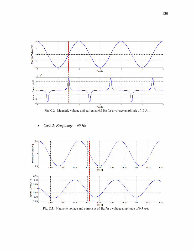
130

Case 2: Frequency = 60 Hz

Fig. C.2. Magnetic voltage and current at 0.5 Hz for a voltage amplitude of 10 A·t.

Fig. C.3. Magnetic voltage and current at 60 Hz for a voltage amplitude of 0.5 A·t..

131

Case 3: Frequency = 1 GHz

Fig. C.4. Magnetic voltage and current at 60 Hz for a voltage amplitude of 10 A·t.

Fig. C.5. Magnetic voltage and current at 1 GHz for a voltage amplitude of 100 A·t..

132

Fig. C.6. Magnetic voltage and current at 1 GHz for a voltage amplitude of 900 A·t..

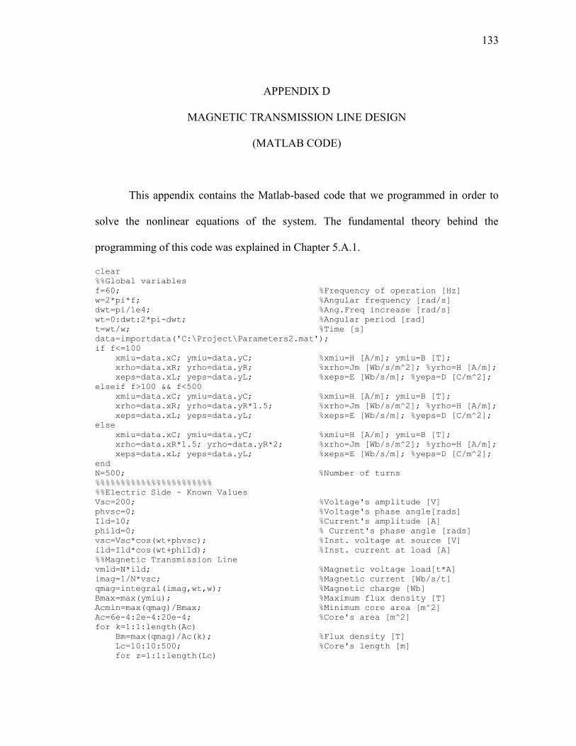
133

APPENDIX D

MAGNETIC TRANSMISSION LINE DESIGN

(MATLAB CODE)

This appendix contains the Matlab-based code that we programmed in order to

solve the nonlinear equations of the system. The fundamental theory behind the

programming of this code was explained in Chapter 5.A.1.

clear

%%Global variables

f=60; %Frequency of operation [Hz]

w=2*pi*f; %Angular frequency [rad/s]

dwt=pi/1e4; %Ang.Freq increase [rad/s]

wt=0:dwt:2*pi-dwt; %Angular period [rad]

t=wt/w; %Time [s]

data=importdata('C:\Project\Parameters2.mat');

if f<=100

xmiu=data.xC; ymiu=data.yC; %xmiu=H [A/m]; ymiu=B [T];

xrho=data.xR; yrho=data.yR; %xrho=Jm [Wb/s/m^2]; %yrho=H [A/m];

xeps=data.xL; yeps=data.yL; %xeps=E [Wb/s/m]; %yeps=D [C/m^2];

elseif f>100 && f<500


xrho=data.xR; yrho=data.yR*1.5; %xrho=Jm [Wb/s/m^2]; %yrho=H [A/m];


else


xrho=data.xR*1.5; yrho=data.yR*2; %xrho=Jm [Wb/s/m^2]; %yrho=H [A/m];


end

N=500; %Number of turns

%%%%%%%%%%%%%%%%%%%%%%%

%%Electric Side - Known Values

Vsc=200; %Voltage's amplitude [V]

phvsc=0; %Voltage's phase angle[rads]

Ild=10; %Current's amplitude [A]

phild=0; % Current's phase angle [rads]

vsc=Vsc*cos(wt+phvsc); %Inst. voltage at source [V]

ild=Ild*cos(wt+phild); %Inst. current at load [A]

%%Magnetic Transmission Line

vmld=N*ild; %Magnetic voltage load[t*A]

imag=1/N*vsc; %Magnetic current [Wb/s/t]

qmag=integral(imag,wt,w); %Magnetic charge [Wb]

Bmax=max(ymiu); %Maximum flux density [T]

Acmin=max(qmag)/Bmax; %Minimum core area [m^2]

Ac=6e-4:2e-4:20e-4; %Core's area [m^2]

for k=1:1:length(Ac)

Bm=max(qmag)/Ac(k); %Flux density [T]

Lc=10:10:500; %Core's length [m]

for z=1:1:length(Lc)

134

xC=xmiu*Lc(z);yC=ymiu*Ac(k); %xC=qm [Wb]; yC=vm [t*A]

xR=xrho*Ac(k);yR=yrho*Lc(z); %xR=im [Wb/s]; yR=vm [t*A]

xL=xeps*Lc(z);yL=yeps*Ac(k); %xL=im [Wb/s]; yL=qe [C]

vcmag=interp1(yC,xC,qmag,'linear'); %Cap's magnetic voltage [t*A]

vrmag=interp1(xR,yR,imag,'linear'); %Res's magnetic voltage [t*A]

flmag=interp1(xL,yL,imag,'linear'); %Ind's electric charge [C]

vlmag=derivate(flmag,t); %Ind's magnetic voltage [t*A]

vmtl=vcmag+vrmag+vlmag; %MTL's voltage [t*A]

vmsc=vmld+vmtl; %Magnetic voltage at source [t*A]

Pmtl=mean(vrmag.*imag); %Real power [W]

%%Electric Side

isc=1/N*vmsc; %Electric current at source [A]

vld=N*imag; %Electric voltage at load [V]

%%%%Efficiency

Psc=mean(vsc.*isc); %Real power at source [W]

Pld=mean(vld.*ild); %Real power at load [W]

Ef(k,z)=Pld/Psc*100; %Efficiency [%]

%%%%Power Factor

vscrms=max(vsc)/sqrt(2); %Source voltage RMS value [V]

iscrms=sqrt(sum(isc.^2)/length(isc)); %Source current RMS value [A]

Ssc=vscrms*iscrms; %Apparent power at source [VA]

PF(k,z)=Psc/Ssc; %Power factor

end

end

clc

135

VITA

Guadalupe Giselle González Domínguez received her Bachelor of Science

degree in electromechanical engineering from the Universidad Tecnológica de Panamá,

Panama City, Panama in 2004.

Professionally, she has worked in the commercialization department of Bahía Las

Minas Corporation, a Panamanian utility company. Since 2006 she has worked as an

assistant researcher assigned to the Office for Research at the Universidad Tecnológica

de Panamá.

She entered the Department of Electrical Engineering at Texas A&M University

in Fall 2006 in order to pursue her doctoral studies and graduated with her Ph.D. in

August 2011. Her areas of interest include: electromagnetic theory, design and control of

electric machines, computer-aided design, sustainable and renewable energy systems,

and power electronics.

Dr. González can be reached at the Electric, Mechanic and Industry Research and

Innovation Center (Centro de Investigación e Innovación Eléctrica, Mecánica y de la

Industria, CINEMI) at the Universidad Tecnológica de Panamá, Panama City, Panama,

e-mail: [email protected] or through her advisor Dr. M. Ehsani at the

Power Electronics and Motor Drives Laboratory, Electrical Engineering Department,

Texas A&M University, College Station, Texas 77843-3128.

mailto:[email protected]

power-invariant magnetic system...

Documents