power quality metrics calculations for the smart grid · power quality metrics calculations for the...

1

Power Quality Metrics Calculations for the Smart

Grid

Second Semester Report

Spring Semester 2013

-Full Report-

By:

Omar Sayied

James Spaulding

Basier Akbary

Prepared to partially fulfill the requirements for ECE402

Department of Electrical and Computer Engineering

Colorado State University Fort Collins, Colorado 80523

Project advisor: Sid Suryanarayanan

Approved by Dr. Sid Suryanarayanan

2

Abstract

The main goal of this project was to create a software system that analyzed data collected from smart meters and alerted the user of power quality issues. Power quality, for the purposes of this project, will be defined as IEEE Std 1159 states, “a wide variety of electromagnetic phenomena that characterize the voltage and current at a given time and at a given location on the power system.” Power quality metrics are defined by a percentage variance from the nominal value over a period of time. The metrics focused on in this report were limited by the resolution of data collected from the smart meters, which was 16.67 ms. This resolution allowed us to analyze disturbances including voltage sags, voltage swells, and harmonics (these disturbances will be further discussed in the body of the report). Along with these disturbances, we also found intervals in the data where low power factor (PF) was of concern. During phase one; we researched definitions, causes, and effects of the aforementioned disturbances. From this, we determined that the best approach to classify these issues would be to use the per-unit system and classify them according to parameters set for power quality issues described in IEEE Std 1159. Once enough data was collected, algorithms were written to extract the data from a comma separated value (.csv) file and uploaded into MatLab. Once the data was uploaded into MatLab, techniques such as the fast Fourier transform (FFT) and averaging sliding window were carried out to locate disturbances. The FFT gave us a means to traverse between the time domain and the frequency domain. The averaging sliding window acted as a low pass filter and got rid of noise that would otherwise flag the beginning of a disturbance haphazardly, ultimately slowing down our algorithms. The algorithms were written as functions, tested and compared with known results from other sources, and then added to a graphical user interface (GUI). The GUI was designed to logically allow any user to plot and textually output any power quality issues, found within our resolution limits, for their own inspection.

3

TABLE OF CONTENTS

Title 1

Abstract 2

Table of Contents 3

List of Figures 4

List of Tables 5

I. Introduction 6

II. Smart Meters 8

III. Ethical Concerns Surrounding Smart Meters 9

IV. Effective Values 10

V. Harmonics 12

VI. Power Factor 14

VII. Voltage Disturbances 15

VIII. IEEE Standards for Power Quality Issues 17

IX. Per-Unit System 18

X. Windowed Fast Fourier Transforms 19

XI. Project Software and Challenges 21

XII. Testing and Methodology 24

• Power Factor 27

• Voltage Sag/Swell 28

• Harmonics 29

XIII GUI Interface 31

XIV. Conclusions and Future Work 33

References 35

Appendix A - Abbreviations 37

Appendix B - Budget 37

Appendix C – Project Timeline 38

Appendix D - Code 41

4

LIST OF FIGURES

Figure 1 RF Exposure study performed by the City of Fort Collins 9

Figure 2 Circuit with AC supply and resistive load. 10

Figure 3 Output voltage waveform through resistive load generated in MatLab 10

Figure 4 Output voltage waveform for power generated in MatLab 11

Figure 5 Three-phase motor rotating coils through magnetic field 12

Figure 6 Maximum flux through surface 13

Figure 7 Voltage distortion between fundamental waveform and 5th harmonic 13

Figure 8 Power triangle 14

Figure 9 Leading and lagging currents; phasor rotation rotates counterclockwise. 14

Figure 10 Total power factor represented by the cos𝜃 in the power triangle 14

Figure 11 Voltage Sags 15

Figure 12 Under voltage 15

Figure 13 Voltage Swells 16

Figure 14 Overvoltage 16

Figure 15 The windowed FFT 19

Figure 16 Customizable Interface 21

Figure 17 Eaton Power Xpert Meter Interface 22

Figure 18 Ranger PM3000 meter with Pronto software kit 23

Figure 19 Apparent power captured on the Pronto meter 23

Figure 20 Pronto apparent power measurements 25

Figure 21 Excel data output 27

Figure 22 MatLab power factor output 27

Figure 23 MatLab power factor graph 27

Figure 24 Excel data voltage output 28

Figure 25 MatLab voltage sag output 29

Figure 26 MatLab Power Spectral Density plot 29

Figure 27 MatLab Harmonics plot 30

Figure 28 Main screen of GUI 31

5

LIST OF TABLES

Table 1 Fundamental frequency of 60 Hz and its harmonic values 12

Table 2 IEEE Categorized Voltage Disturbances 17

Table 3 Some applications of the WFFT analysis 20

Table 4 ION Setup stored data 22

Table 5 Maximum and minimum values of captured momentary voltage swell 26

6

Chapter 1: Introduction

A good way to measure the power quality is to compare the voltage and current wave-shapes to an ideal sinusoid of the desired nominal frequency and magnitude. Since establishments push to keep the waveforms of their power systems as close as possible to a nominal level, any variation of waveforms from the nominal waveform may be considered a power quality issue. With the rise in high-power semiconductor switches, non-sinusoidal load currents have become more common [1]. Proper management of new integration techniques such as wind and solar, which introduce non-sinusoidal waveforms due to power electronic interfaces, is necessary to mitigate issues relating to power quality. However, to mitigate any power quality problem, it is necessary to quantify the deviation from ideal conditions. We use metrics that are commonly in practice on data gathered from meters to quantify the loss of power quality.

Power quality indices are used to measure the quality of the power supply. Some of the best known indices are the following: total harmonic distortion (THD), PF, telephone influence factor (TIF), flicker factor (FF), and unbalance factor (UF). Due to the resolution of data from the smart meters, our indices were limited to THD and PF. Within these indices, the phase voltages and currents were analyzed for harmonics, disturbances, and low PF.

Voltage sags, voltage swells, harmonics, and a low power factor greatly contribute to a decrease in power quality and it is important for entities to closely monitor these phenomena. Utility power companies charge their customers for lower power quality, therefore entities will want to continuously monitor their overall power quality to ensure that it is at an optimal value. Monitoring the power quality will provide the entity with the prospect of ensuring that their power grid is efficiently delivering power. Due to the fact that there are multiple motors, generators, air conditioning units, heaters, refrigerators, etc. in entities that own large buildings, it is important that they keep their power quality as efficient as possible. They will be able to save a lot of money while at the same time slightly cutting back on the total pollution that can result from having low power quality. In detail, cutting losses on transmission, distribution, and utilization of total power reduces power supply generation which in result, helps cut back on pollution. The common format of the data that was extracted from the power meters was in the .csv format. This format separates the data with a comma as the delimiter. We opened the .csv data sheet in Excel which properly placed the data in respective columns. After the data had been put into excel form, for easier understanding, we then analyzed it through MatLab using algorithms. Our system stored each column, which represents a variable, from the input data into a separate database of arrays. MatLab then ran through the array and analyzed each value according to the characteristics defined by IEEE Std 1159. Once the algorithms were tested and properly outputting desired results, they were put into a GUI designed in MatLab. The GUI gives the user the ability to upload data files and find power quality issues if any exist. The algorithms were written for the finest resolution obtained by the meters and were manipulated to classify varying events where a power quality issue was present. By changing the time parameters classifying an event, the same algorithm was used to find another classification of an event since the equations used to characterize an issue are solved similarly.

7

This report will examine common areas and variables that distort power quality. Some variables include effective values, harmonics, and power factor. The most common disturbances seen in a power system will be defined and analyzed, such as voltage sags and swells. With the aid of IEEE standards, specifically IEEE 1159 and IEEE 519, harmonics and disturbances are properly categorized and further analyzed.

After the standards are generalized, a concise explanation of the importance of per unit analysis and its importance regarding this project are presented. The later parts of the report include a brief introduction to a sampling technique that helps speed up the algorithms known as the windowed FFT. Following this, new metering devices known as smart meters are described and a brief mention of ethical concerns currently surrounding smart meters is introduced. Next, the report will detail testing performed and give a brief synopsis of what issues we found. The GUI design and algorithmic implantation into the GUI are both described. Lastly, the report concludes with recommendations and plans for future work.

8

Chapter 2: Smart Meters

A smart meter is a device that monitors power consumption with two-way communication. Users can access detailed information about their energy use and power quality. This includes services like monitoring energy consumption, voltage and power ratings, and warning measures against power quality issues. It also provides faster and more reliable service from the energy companies to the users. In the event of a power outage, for example, the energy company will be alerted instantly so they can identify and resolve the problems in a timely manner.

Smart meters are being integrated into the North American power grid’s secondary power distribution environment to better monitor power usage. Old meters that strictly monitor kilowatt hour usage for electric utility companies billing purposes are being replaced with smart meters which offer both the customer and the supplier more monitoring options and data. The data the smart meters acquire is being used to show customers their overall power consumption, how they consume power, and better inform them of ways they may be able to reduce their consumption. Power companies will be able to use the finer resolution of data to better supply loads during peak intervals. The ultimate goal of the smart meter is to increase efficiency of power supplied, allow new power generation techniques to be integrated into the distribution level, and reduce excessive power consumption through awareness.

Smart meters use radio frequency (RF) to relay information from the meter to the customer in real-time. They are part of a network that can receive software and firmware update remotely, thus reducing the need for scheduling technician appointments. More advanced uses for smart meters are to monitor power quality parameters like voltage disturbances, harmonics and power factor. With this kind of information, power companies have a better understanding of the quality of power that their customers are receiving and can act upon any unwanted observations. Smart meters equip power companies with additional information that can aid them in resolving any issues that crop up.

9

Chapter 3: Ethical Concerns Surrounding Smart Meters

The smart meter relays the data it collects about how consumers use power, when they use it, and are able to decipher which devices may be running from the higher resolution of data collected. Basically, the consumer’s once private consumption of power is now completely exposed to the electric utility company. As households start communicating to the power grid, some questions that raise concerns are: Who will be monitoring the information? What can be exposed from the information? In a way, it can be seen as violating the fourth amendment, which is often interpreted as the right to privacy Smart meters allow for a real time reading of power usage. Since smart meters collect real time data, people can determine how many people live in a household, the times when nobody is home, type of equipment in the home, and specific changes in daily routines just from the data collected from the smart meters connected to a house. One of the biggest concerns is the fact that they can track whether a family is at home, on a holiday, or at work. The privacy in which most households currently have could quickly disappear with the installation of smart meters and smart power grids.

Moreover, health and safety concerns regarding human radio frequency (RF) exposure have been questioned by concerned customers. Smart meters use radio frequency to communicate with the central system. Radio frequency is a type of electromagnetic radiation which is known to have the potential of overheating cells in the human body when transmitting in close range. The cells are unable to dissipate heat and are destroyed. However, the RF emission from a smart meter is low and nearly negligible compared to a cell phone, for instance.

Despite the opposition, the overall trend in smart meters is increasing. More communities are having smart meters installed as they evolve with advanced technology. Essentially, there are more good features that smart meters provide than unwanted characteristics that assailants express.

Figure 1: RF Exposure study performed by the City of Fort Collins [21]

10

(s)

Figure 2: Circuit with AC supply and resistive load. [20]

Figure 3: Synthetic data representing the output voltage waveform through resistive load generated in MatLab.

0 20 40 60 80 100 120 140 160 180 200-1

-0.5

0

0.5

1

t

V(t

)

Chapter 4: Effective Values

To better understand the values used in power systems, we must first understand what the effective values are. To describe the effective value, we will use an example to define effective voltage. The reader should be aware that the method to find the effective voltage will be identical to the method for finding the effective current.

The effective value is also referred to as the rms value. Using this term will give us a better understanding of what the effective value is. We will use a simple example of a circuit with a resistive load shown in figure 2. Considering just the waveform of the voltage through the resister, we will see a plot as in figure 3. The waveform alternates between positive and negative volts. Instantaneous power is found using equation 4.1 below. Using Ohm’s Law, shown in equation 4.2, and solving for the current, we derive a useful equation for instantaneous power considering only voltage and the resister shown in equation 4.3.

𝑃(𝑡) = 𝐼(𝑡)𝑉(𝑡) (4.1)

𝑉(𝑡) = 𝐼(𝑡)𝑅 → 𝐼(𝑡) = 𝑉(𝑡)𝑅

(4.2)

𝑃(𝑡) = 𝑉(𝑡)2

𝑅 (4.3)

Looking at only the numerator of equation 4.3, we plot the voltage in figure 4. To find the total amount of energy in this waveform, we take the average voltage over one period. To find the average we sum all of the energy up under the curve and divide by the period of the summed amount of energy, shown in equation 4.4.

1𝑇 ∫ 𝑉(𝑡)2𝑇

0 𝑑𝑡 (4.4)

11

(s) 0 20 40 60 80 100 120 140 160 180 2000

0.2

0.4

0.6

0.8

1

t

V(t

)2

Now, we would like to find an effective voltage that will represent a direct current (DC) value. To do this, we use equation 4.5.

𝑃 =𝑉𝐸𝑓𝑓2

𝑅 (4.5)

𝑉𝐸𝑓𝑓2 = 1𝑇 ∫ 𝑉(𝑡)2𝑇

0 𝑑𝑡 (4.6)

𝑉𝐸𝑓𝑓 = �1𝑇 ∫ 𝑉(𝑡)2𝑇

0 𝑑𝑡 (4.7)

Setting the effective voltage equal to our average, or mean voltage, we are able to derive a value for the effective voltage which relates the DC value and AC value together. For the rest of the text we will use E to represent effective voltage.

An even easier relation between the AC rms value and the DC value is found by solving the integral. Since we are dealing with the cosine component of the voltage throught the resister, we can solve equation 4.7 and get the result shown in equation 4.8.

𝐸 = 𝑉𝐸𝑓𝑓=�1𝑇 ∫ 𝑉(𝑡)2𝑇

0 𝑑𝑡 = �1𝑇 ∫ 𝑉(𝑡)2𝑐𝑜𝑠2𝜃𝑇

0 𝑑𝑡 = 𝑉(𝑡)√2

(4.8)

The same result will be found for the effective current represented by equation 4.9.

𝐼 = 𝐼(𝑡)√2

(4.9)

The important relation between the DC and AC rms value is that they share the same amount of energy although their amplitudes are different. This means that the effective AC voltages share the same thermal limitations and ability to carry superimposed harmonics as the DC voltages.

Figure 4: Synthetic data representing the output voltage waveform for power generated in MatLab.

12

Table 1: Fundamental frequency of 60 Hz and its harmonic values.

Chapter 5: Harmonics

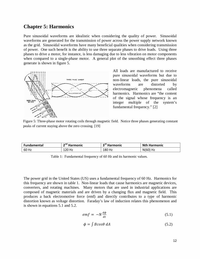
Pure sinusoidal waveforms are idealistic when considering the quality of power. Sinusoidal waveforms are generated for the transmission of power across the power supply network known as the grid. Sinusoidal waveforms have many beneficial qualities when considering transmission of power. One such benefit is the ability to use three separate phases to drive loads. Using three phases to drive a motor, for instance, is less damaging due to less vibration on motor components when compared to a single-phase motor. A general plot of the smoothing effect three phases generate is shown in figure 5.

All loads are manufactured to receive pure sinusoidal waveforms but due to non-linear loads, the pure sinusoidal waveforms are distorted by electromagnetic phenomena called harmonics. Harmonics are “the content of the signal whose frequency is an integer multiple of the system’s fundamental frequency.” [2]

The power grid in the United States (US) uses a fundamental frequency of 60 Hz. Harmonics for this frequency are shown in table 1. Non-linear loads that cause harmonics are magnetic devices, converters, and rotating machines. Many motors that are used in industrial applications are composed of magnetic materials and are driven by a changing flux and magnetic field. This produces a back electromotive force (emf) and directly contributes to a type of harmonic distortion known as voltage distortion. Faraday’s law of induction relates this phenomenon and is shown in equations 5.1 and 5.2.

𝑒𝑚𝑓 = −𝑁 𝑑𝜙𝑑𝑡

(5.1)

𝜙 = ∫𝐵𝑐𝑜𝑠𝜃 𝑑𝐴 (5.2)

Fundamental 2nd Harmonic 3rd Harmonic Nth Harmonic 60 Hz 120 Hz 180 Hz N(60) Hz

Figure 5: Three-phase motor rotating coils through magnetic field. Notice three phases generating constant peaks of current staying above the zero crossing. [19]

13

Figure 7: Voltage distortion between fundamental waveform and 5th harmonic. [4]

To achieve the greatest flux (𝜙), motors are built to have zero angle between the surface area vector (

𝒅𝑨��) and the magnetic field vector (

𝑩→). To better understand figure 5 is provided below.

The emf sends a voltage out onto the distribution lines creating a voltage distortion. This causes inefficiency in the power flow of the grid. In fact, “Industry and infrastructures consume more than 31% of the available energy and electrical motors, alone, represent more than 60% of this.”[3] Voltage distortion may be seen in figure 6. Voltage distortion is composed of the sum of all harmonics and the fundamental sinusoid. Equation 5.3 is used to calculate distorted voltage.

𝐸 = �𝐸𝐹2 + 𝐸𝐻2 (5.3)

𝐸𝐻 = �𝐸22 + 𝐸32 + ⋯+ 𝐸𝑁2 (5.4)

Equation 5.4 represents the total amount of effective voltage harmonics present. The relationship for effective currents is derived exactly the same as for effective voltages. When describing the harmonic distortion we may consider the total effective voltage distortion or the total effective current distortion. Both describe the total harmonic distortion (THD).

To describe the amount of distortion for voltages or currents we will use the THD. The THD is the “effective value of all the harmonics divided by the effective value of the fundamental.”[4] This is shown in equation 5.5.

𝑇𝐻𝐷 = 𝐸𝐻𝐸𝐹

=�𝐸22+𝐸32+⋯+𝐸𝑛2

�𝐸2−𝐸𝐻2

(5.5)

Harmonics are a leading cause of power quality issues in areas where non-linear loads are concerned. The values of THD will be classified and categorized according to standard IEEE 1159 and analyzed by techniques described in standard IEEE 519 discussed in chapter 8.

𝐵→

𝑑𝐴��

Figure 6: Maximum flux through surface

14

Chapter 6: Power Factor

Power factor is a term used to describe the ratio of quality power divided by the apparent power in the system. The power factor will be one of our main alerting variables to identify a possible power quality issue. The power factor is composed of two components; a distortion component and a displacement component. The displacement component is, by definition,” the ratio of the active power of the fundamental wave, in watts, to the apparent power of the fundamental wave, in volt-amperes.”[5]. The best way to describe this is by using the power triangle shown in

figure 8.

𝑃 = 𝐸𝐼𝑐𝑜𝑠𝜃 (6.1)

𝑄 = 𝐸𝐼𝑠𝑖𝑛𝜃 (6.2)

𝑆 = �𝑃2 + 𝑄2 (6.2)

Figure 8: Power triangle

Displacement power factor only considers the fundamental waveforms and is related to how much reactance is in the system which is denoted by the Q in the power triangle. Reactance comes from the amount of phase difference between the voltage and the current. When the current is leading the voltage, we see a capacitive load. When the current is lagging the voltage, we see an inductive load. Both of these instances are shown in figure 9.

The cosine of 𝜃 in the power triangle is the total power factor. The total power factor takes into account the distortion component along with the displacement component. The distortion component contains all of the harmonics in the voltages and currents. Refer to chapter 5 equations 5.3-5.5 for a discussion on voltage distortion.

Figure 9: Leading and lagging currents; phasor rotation rotates counterclockwise.

Figure 10: Total power factor represented by the cos𝜃 in the power triangle.

15

Chapter 7: Voltage Disturbances

The most commonly encountered phenomena in a power system are the occurrence of a voltage sag or voltage swell. A voltage sag is defined as the incidence where the RMS voltage is less than the nominal voltage at the power frequency (60 Hz) of a power system. IEEE 1159 defines a voltage sag as a value that is 10% to 90% of the nominal voltage of the system that lasts from 0.5 cycles to 1 minute. Voltage sags are typically caused by sudden increases in the load or the starting of motors, refrigerators, etc [7]. They can also be caused by a loose connection, short circuit, fault in a circuit, or by induction motors that draw a large amount of current during startup [2]. The large amount of drawn current causes a drop in voltage across the impedance of the circuit which is classified as a voltage sag. Long duration voltage sags, or voltage sags that last longer than 1 minute are referred to as under voltages. Under voltages in a system can cause malfunctions in motors and appliances that require a fixed amount of power to operate nominally. When the voltage in motors or appliances decrease, the current must increase to supply the same amount of power, if the current increases above the current rating for the motor or appliance, it can increase heat and damage the motor or appliance. Voltage sags ultimately lead to a decrease in efficiency and power quality of a power system.

Figure 11: Voltage Sags [7]

The two figures above represent an instantaneous voltage sag (upper figure) and a voltage sag that lasts more than one cycle (lower figure). As can be seen, the magnitude of the voltage during the voltage sag is much lower than the nominal magnitude.

Figure 12: Represents an under voltage due to the fact that the voltage sag lasts for more than 1 min. [12]

t > 1 min

16

A voltage swell is defined as an occurrence where the RMS voltage is more than the nominal voltage at the power frequency of a power system. IEEE 1159 defines a voltage swell as a value that is 110% to 180% of the nominal voltage of the system that lasts from 0.5 cycles to 1 minute. Voltage swells are typically caused by an instant reduction in the load of a circuit. Long duration voltage swells, or voltage swells that last longer than 1 minute, are referred to as over voltages. Over voltages in a system can also damage or cause malfunctions in motors or appliances. If the input voltage drastically increases above the max voltage rating of a motor or appliance, it will increase the heat in the motor or appliance and either damage internal parts or drastically shorten its life.

Figure 13: Voltage Swells [7]

The two figures above represent an instantaneous voltage swell (upper figure) and a voltage swell that lasts more than one cycle (lower figure). As can be seen by the two red lines on the lower figure, the magnitude of the voltage is about 10% higher than the nominal magnitude.

Figure 14: Represents an overvoltage due to the fact that the voltage swell lasts for more than 1 min. [13]

t > 1 i

17

Chapter 8: IEEE Standards for Power Quality Issues

Industry standards provide common guidelines for manufacturers and designers to refer to. By doing this, a universal understanding of characteristics, design specifications, or maintenance techniques are followed across all industries involved in the same market. This makes integration of new components into an existing system considerably manageable. Regarding power quality issues, IEEE Standard 1159 is a useful resource for classifying different types of issues, monitoring techniques, and expresses the importance of monitoring. IEEE Standard 519 provides a detailed discussion on harmonics and offers varying techniques for quantifying them, what causes them, and suggests mitigation strategies.

There are four different classifications of voltage sags and swells: instantaneous, momentary, temporary, and long duration [7]. Each of the classification standards are defined in terms of per-unit. Our system followed table 2 for classifying the different types of sags and swells in terms of magnitude and duration. To put the chart below into perspective, a voltage swell with a magnitude that is 1.3 times the nominal voltage value and lasts 2 seconds will be classified as a 'momentary swell.'

Table 2: IEEE Std. 1159 Categorized Voltage Disturbances [7]

18

Chapter 9: Per-Unit System

Our code will be designed to use the Per-Unit System of Units for calculation of the metrics. The per-unit system allows for computation of variables in terms of fractions of a predefined base quantity. For example, if the nominal magnitude of a voltage in a power system is 100V and a voltage sag occurs which decreases the voltage to 90V then the per-unit representation of the voltage would be 90V/100V = 0.9 p.u. (per-unit). This allows for much easier calculation and code generation, by converting all components, regardless of the magnitude, to the same unit system in terms of a fraction.

The per-unit system is commonly used in power engineering designs. By using per unit analysis, devices such as electrical motors, generators, and transformers become normalized by the circuit’s base rating. The base rating is typically defined in MVA and allows circuit diagrams to be reformatted into one-line diagrams. All of the information provided in a complex circuit design is transferred to a less complicated one-line diagram. From this, the user will be able to gain the same amount of knowledge about the circuit in a more manageable fashion.

Our first approach was to calculate the percentage change between the nominal voltage magnitude and the voltage sag/swell magnitude, then determine whether the percentage change was large enough to be classified as a sag or a swell. For example, if we classified a 5% deviation in voltage magnitude as a sag/swell where the nominal voltage equals 100 volts and the voltage at a specific point equals 97 volts, then the deviation would be 97/100 or 3%. Therefore, in this case, there would be no voltage sag because the deviation is not 5% or greater.

After further research and consideration, we determined that the best approach would be to convert the input data to the per-unit system and then use the IEEE 1159 standards chart shown in Table 2 to determine which classification the voltage sag or swell fell under. This in turn helped us determine the severity of the voltage sag or swell that was detected in the data provided by the meters.

19

Chapter 10: Windowed Fast Fourier Transforms

One challenge in power quality assessment is the large volume of data that is stored and analyzed. Three phase currents, three phase voltages, neutral currents, and neutral to ground voltages need to be stored at a high sample rate, generally 5 kHz, over long periods of time. The key is to analyze the data as fast as possible while being as accurate as possible when it counts. One approach to this challenge is to use the discrete Fourier transform. The Fourier transform is a method used to transfer functions from the time domain to the frequency domain and vise versa. The discrete Fourier transform function is shown in (10.1).

𝐹(𝑘∆𝛺) = � 𝑓(𝑖∆𝑇)𝑒−𝑗𝑘𝑖∆𝛺∆𝑇𝑁−1𝑖=0 (10.1)

where ∆𝛺 is the resolution in frequency domain and ∆𝑇 is the sample rate of f(t). For power quality analysis, the discrete Fourier transform will use a sliding, adjustable window technique, where N-1 is the window length.

In order to analyze large data volume efficiently, speed needs to be a priority. For speed analysis, the FFT will use a large window size with a slow sample rate. However, the sample rate must be fast enough to capture high frequency events. Once it does capture a disturbance, the window is shortened and the sample rate is increased to get a very accurate analysis of the phenomena. After the disturbance is analyzed, the window length and sample rate will be adjusted for rapid analysis when no high frequency phenomena are present. This process is illustrated in the figure below.

Figure 15: The windowed FFT [6].

The WFFT analysis does introduce some errors that need to be accounted for. Some of these errors can be limited by selecting proper parameters (e.g. sample time and window length) and applying digital filters to suppress noise. One of the obstacles is speed versus accuracy. As explained earlier, based on the window length and sample rate parameters, a trade-off between speed and accuracy is created. Another obstacle is edge data. At the edge of a disturbance, the window will contain both normal and disturbance amplitudes. This cannot be analyzed by the FFT so that data is discarded. Aliasing is a third obstacle with the WFFT. When the sample rate is too low, the high frequency components are translated into lower frequencies. This error can

20

be avoided by increasing the sampling frequency. Because the FT analysis is truncated in the time domain, leakage will occur in the frequency domain. Leakage is another barrier that spreads energy from one frequency to another. Setting an integer number of cycles in each window, however, will remove all leakage. The last important hurdle is the picket-fence effect, which is like looking at the data through a picket fence. This happens when the desired frequency is not an integer multiple of the fundamental frequency. A frequency in the nth and (n+1)th harmonics will affect the magnitudes. A technique to reduce this effect is to increase the resolution of the analysis.

The application for the WFFT analysis is to locate and categorize disturbances. The disturbances are classified and categorized beyond the WFFT analysis, based on the IEEE 1159 Standard. Some practical events are shown in the table below. From these events, the WFFT can analyze the specified power quality voltage and current problems. For example, in the event of a fault, the WFFT can analyze the voltage sags and neutral currents caused by it. Note that both current types include nonlinear load types and transformer saturation.

Table 3: Some applications of the WFFT analysis [6].

One alternative to power quality assessment is wavelet analysis. Wavelet analysis is similar to the WFFT analysis in that it uses large wavelets to analyze low frequency effects such as flicker and small wavelets to analyze high frequency, short term effects such as momentary outages and fast transients. A benefit to wavelet analysis is it gives accurate dilation and shift data that the WFFT does not. However, wavelet analysis does not generate any frequency data like phase and magnitude. Therefore, the WFFT analysis is preferred.

21

Chapter 11: Project Software and Challenges

Our original customer planned for us to use the smart meter software, StruxureWare Power Monitoring 7.0. This software exports a Microsoft Structured Query Language, or MS SQL, database that contains key data points like voltages and currents. The software has a customizable interface that can display dashboards, diagrams, tables, alarms and reports. The figure below shows an example of a dashboard through SPM7.

Figure 16: SPM7 Customizable Interface [8]

However, we ran into some difficulties with our customer as he was transferred to another state with a new project. Therefore, our senior design group needed to look for other power meters locally and work with those instead.

We setup a meeting with the CSU head of power metering, Chuck Sawyer, and gained access to the ION and Eaton meters installed on campus. The ION meters used the power quality measuring program, ION Setup, which is a very basic form of power monitoring. These meters sampled key variables like voltages, currents, power factor and harmonics and uploaded and displayed them every second through the secure online CSU site. ION Setup only stored a limited amount of data at a low resolution. It stored the real and reactive power measured every 15 minutes for the last three months, and it stored any information regarding voltage sags and swells that occurred during those three months. This software created some challenges for us because we had to manually record most of the data ourselves. This process made it difficult to obtain data at quick sample rates. We avoided these meters because of the lack of useful data it provides. An example table output that ION Setup provides is shown in table 4.

22

Table 4: ION Setup stored data

The Eaton meters used a program called Power Xpert Meter. We accessed this program through the secure CSU site like ION Setup. Power Xpert Meter was a more advanced software that plotted and exported much more data than ION Setup. We had some difficulties in accessing the full Power Xpert Meters software through the secure site because of a Java error we obtained and could not find a solution for. We have asked Chuck if he knows of any workarounds to the error and we implemented his suggestions but it did not help. We could access the software without Java active, but we only get access to very basic information like the three phase voltages and currents, power factor and frequency. This basic information was updated every 10 seconds and the stored data could not be accessed without Java. Eaton did have a live demo of their software actively monitoring on their website. Therefore, we used the Eaton site to get more acquainted with the software and know exactly the type of data it export. In the end, we extracted some of our data for our code from the Eaton live demo site. The figure below shows the user interface of Power Xpert Meters and an example of the plots it provides.

Figure 17: Eaton Power Xpert Meter Interface [9]

23

Later, we got access to another power meter supplied by the city of Fort Collins. This was the Ranger PM3000 smart meter using Pronto software for Windows. They can be configured to log specific data or data from a certain time window. Pronto for Windows allowed graphing, analyzing and creating hard copy reports of the data it monitors. A photo of the meter kit we used is shown on the left.

Figure 18: Ranger PM3000 meter with Pronto software kit

We configured Pronto to record ten days worth of data. The Pronto data logger allowed us to get plots for real and reactive power and any voltage swells that occurred. Pronto exported a comma separated value (.csv) file that logged all three phase AC RMS voltages and currents, real and apparent power readings every one second for a 24 hour period. We also extracted higher resolution readings of the real and apparent power over a duration of one hour with 16.67 ms intervals. A plot showing the apparent power measured during the ten day period is shown in the figure below.

Figure 19: Apparent power captured on the Pronto meter

With access to these three different meters, it gave us many options on how to progress this project. We ended up using the Pronto recordings for most of our code and relied on the high resolution Eaton recordings for our harmonics analysis code.

24

Chapter 12: Testing and Methodology

The testing we performed on the code that monitors the power factor involved the testing of large data files. Our system was able to input and analyze large data files and determine all of the points in which the power factor dropped below 0.8 as specified by our customer. We tested the system with smaller time values and the results were as we expected.

We also used the Pronto metering software to test our functions by using archived data provided by the City of Fort Collins data logs. The City of Fort Collins metering department installed Ranger meters on a local industry in 2011 to analyze the load their machines were drawing from the local grid. We used this data to capture disturbances within our resolution limits. The following provides an example of capturing and classifying a momentary voltage swell. To do this we requested varying time intervals and were able to zoom in to the disturbance down to the millisecond. A step by step zoom in is shown in figure 19.

25

Figure 20: Apparent power measurements

26

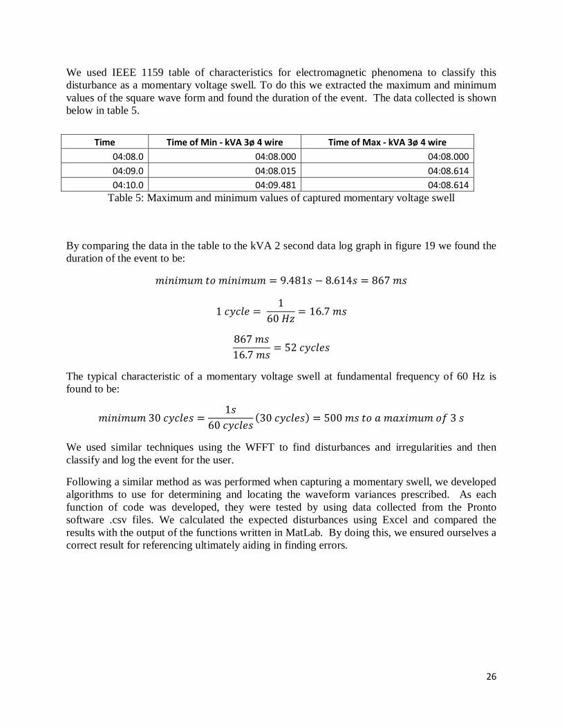
We used IEEE 1159 table of characteristics for electromagnetic phenomena to classify this disturbance as a momentary voltage swell. To do this we extracted the maximum and minimum values of the square wave form and found the duration of the event. The data collected is shown below in table 5.

Table 5: Maximum and minimum values of captured momentary voltage swell

By comparing the data in the table to the kVA 2 second data log graph in figure 19 we found the duration of the event to be:

𝑚𝑖𝑛𝑖𝑚𝑢𝑚 𝑡𝑜 𝑚𝑖𝑛𝑖𝑚𝑢𝑚 = 9.481𝑠 − 8.614𝑠 = 867 𝑚𝑠

1 𝑐𝑦𝑐𝑙𝑒 = 1

60 𝐻𝑧 = 16.7 𝑚𝑠

867 𝑚𝑠16.7 𝑚𝑠 = 52 𝑐𝑦𝑐𝑙𝑒𝑠

The typical characteristic of a momentary voltage swell at fundamental frequency of 60 Hz is found to be:

𝑚𝑖𝑛𝑖𝑚𝑢𝑚 30 𝑐𝑦𝑐𝑙𝑒𝑠 =1𝑠

60 𝑐𝑦𝑐𝑙𝑒𝑠(30 𝑐𝑦𝑐𝑙𝑒𝑠) = 500 𝑚𝑠 𝑡𝑜 𝑎 𝑚𝑎𝑥𝑖𝑚𝑢𝑚 𝑜𝑓 3 𝑠

We used similar techniques using the WFFT to find disturbances and irregularities and then classify and log the event for the user.

Following a similar method as was performed when capturing a momentary swell, we developed algorithms to use for determining and locating the waveform variances prescribed. As each function of code was developed, they were tested by using data collected from the Pronto software .csv files. We calculated the expected disturbances using Excel and compared the results with the output of the functions written in MatLab. By doing this, we ensured ourselves a correct result for referencing ultimately aiding in finding errors.

Time Time of Min - kVA 3ø 4 wire Time of Max - kVA 3ø 4 wire 04:08.0 04:08.000 04:08.000 04:09.0 04:08.015 04:08.614 04:10.0 04:09.481 04:08.614

27

Power Factor

We calculated the power factor by using (12.1).

𝑃𝐹 = 𝑅𝑒𝑎𝑙 𝑃𝑜𝑤𝑒𝑟𝐴𝑝𝑝𝑎𝑟𝑒𝑛𝑡 𝑃𝑜𝑤𝑒𝑟

(12.1)

The power factor at 3538 seconds in the data is PF = 30.4/39.7 = 0.76574307304

Figure 21: Data opened in Microsoft Excel. The second to last column refers to the real power and the last column refers to the apparent power.

Then comparing this value to the value obtained in our code, we can see that they both match. Further testing shows that the plot of the power factor provides the same results referenced in figure 23.

Figure 22: A snippet of the code printed in the MatLab command window for testing purposes. The power factor at 3538 seconds matches the PF calculated above.

Figure 23: Power factor between 3537 and 3539 seconds showing result of approximately 0.76.

3537 3537.2 3537.4 3537.6 3537.8 3538 3538.2 3538.4 3538.6 3538.8 35390.76

0.78

0.8

0.82

0.84

0.86

0.88

0.9

0.92

0.94

28

Voltage Sag/Swell

The nominal voltage is calculated by taking the average every 60 seconds. The nominal voltage value is then compared to the actual voltage at each time stamp.

𝐶𝑎𝑙𝑐𝑢𝑙𝑎𝑡𝑒𝑑 𝑉𝑎𝑙𝑢𝑒: 𝐴𝑐𝑡𝑢𝑎𝑙 𝑉𝑜𝑙𝑡𝑎𝑔𝑒 𝑉𝑎𝑙𝑢𝑒 / 𝑁𝑜𝑚𝑖𝑛𝑎𝑙 𝑉𝑜𝑙𝑡𝑎𝑔𝑒 𝑉𝑎𝑙𝑢𝑒

If the Calculated Value is between 0.1-0.9, then the disturbance is classified as a voltage sag. If the Calculated Value is between 1.1-1.8, then the disturbance is classified as a voltage swell. For precision purposes, we designed our software to classify a voltage sag if it dropped below 0.95 of the nominal voltage, and a voltage swell if it increased above 1.05 of the nominal voltage.

The nominal voltage can be calculated by looking at the integer multiple of 60 seconds that falls in a specific range of data time stamps. The value of the voltage at all 60 seconds is 281.7 except for the values at times 484 and 485 seconds. Therefore the nominal voltage can be calculated by adding all voltages:

58 ∗ 281.7 + 266.7 + 265.7 = 16871

𝑁𝑜𝑚𝑖𝑛𝑎𝑙 𝑉𝑜𝑙𝑡𝑎𝑔𝑒 = 16871/60 = 281.183333333

Figure 24: A snippet from the data opened in Excel.

At points 484 and 485 seconds, the voltage looks to be smaller than the nominal voltage. Therefore, we can calculate if there is a voltage sag at these points. At 484 seconds:

266.7 𝑉𝑜𝑙𝑡𝑠 / 281.183333 𝑉𝑜𝑙𝑡𝑠 = 0.9484914954

As stated earlier, our code was designed to define anything under .95 as a voltage sag. Therefore we should expect a voltage sag at points 484 and 485 seconds (since the voltage at 485 seconds is smaller than the voltage at 484 seconds). We then tested our code to see if the voltage sag at these two time stamps was recognized. Figure 24 was taken from the command window of MatLab after running our code.

Figure 25: Voltage sag output from MatLab

As can be seen, it is found that there is a voltage sag at both of those points.

29

Harmonics

The harmonics for a waveform are calculated by use of the Fast Fourier Transform. We input the current waveform in the data into the fft() function in MatLab to find the harmonics of the waveform. Since the fft() function represents the harmonics in a mirror image, we only looked at the first half of the calculated values. The data is then converted to the frequency domain by utilizing the sampling frequency and length of the data. The sampling frequency can be calculated by the function [frequency = 1/time] where time is the difference between two time values in the data. We used the psd() (Power Spectral Density) function in MatLab to test the harmonics function of the code. The psd() function shows the current waveform in terms of power/frequency in the frequency domain. The figure below is the output of the psd() function.

Figure: 26: Power Spectral Density plot in MatLab

It can be seen that the magnitude of power/frequency increases at the integer multiples of the fundamental frequency (60 Hz). The magnitude is highest at 60Hz, as expected, since it is the fundamental frequency, then there is an increase in magnitude at 180Hz, 300Hz, and 420 Hz. The magnitudes of the harmonics from largest to smallest in terms of frequency are 60Hz, 180Hz, 420Hz, and 300Hz.

Running the harmonics code with the same current wave form data used in the psd() function provides the following figure.

0 50 100 150 200 250 300 350 400 450-10

0

10

20

30

40

50

60

70

Frequency (mHz)

Pow

er/fr

eque

ncy

(dB

/Hz)

PSD of Data

30

Figure 27: Harmonics plot in MatLab

As can be seen, the harmonics occur at the same frequencies, and further analysis shows that magnitudes match the magnitudes obtained in the psd() function. Just looking at the integer multiples of the fundamental frequency, the magnitudes of the harmonics from largest to smallest in terms of frequency are 60Hz, 180Hz, 420Hz, and 300Hz, which match the data obtained above. The Total Harmonic Distortion (THD) is then calculated by the use of the following function:

𝑇𝐻𝐷 =�𝑉22+𝑉32+⋯+𝑉𝑛2

𝑉1 (12.2)

V1 is the RMS voltage at the fundamental frequency. Our code then displays the percentage of Total Harmonic Distortion in the GUI. The snippet below is taken from MatLab, which shows that our system displays the total harmonic distortion of the current wave used above.

>> Harmonics_THD

Total Harmonic Distortion = 3.99886%.

-100 0 100 200 300 400 5000

50

100

150

200

250

300

350

400

450

500

31

Chapter 13: GUI

The GUI was designed to meet the needs of an industrial user. We wanted the user to obtain detailed information about any issue they chose to seek without confusion. To achieve this, 3 main goals were pursued:

• Uncluttered interface • User friendly for all skill levels • Quick and direct

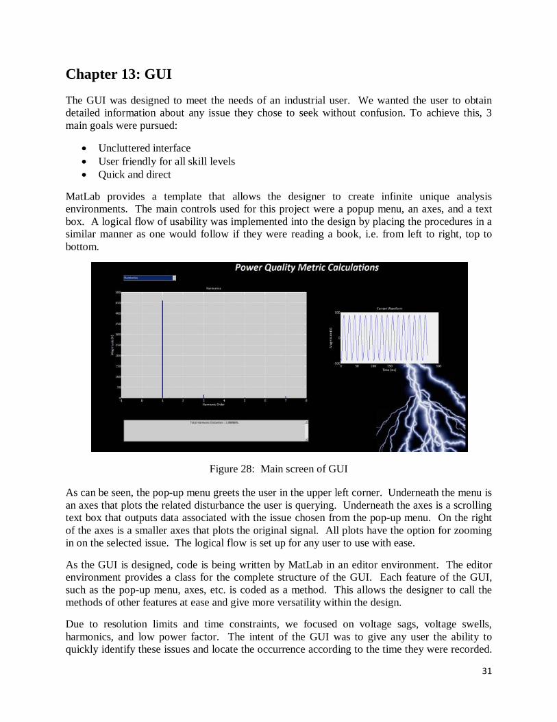
MatLab provides a template that allows the designer to create infinite unique analysis environments. The main controls used for this project were a popup menu, an axes, and a text box. A logical flow of usability was implemented into the design by placing the procedures in a similar manner as one would follow if they were reading a book, i.e. from left to right, top to bottom.

Figure 28: Main screen of GUI

As can be seen, the pop-up menu greets the user in the upper left corner. Underneath the menu is an axes that plots the related disturbance the user is querying. Underneath the axes is a scrolling text box that outputs data associated with the issue chosen from the pop-up menu. On the right of the axes is a smaller axes that plots the original signal. All plots have the option for zooming in on the selected issue. The logical flow is set up for any user to use with ease.

As the GUI is designed, code is being written by MatLab in an editor environment. The editor environment provides a class for the complete structure of the GUI. Each feature of the GUI, such as the pop-up menu, axes, etc. is coded as a method. This allows the designer to call the methods of other features at ease and give more versatility within the design.

Due to resolution limits and time constraints, we focused on voltage sags, voltage swells, harmonics, and low power factor. The intent of the GUI was to give any user the ability to quickly identify these issues and locate the occurrence according to the time they were recorded.

32

One issue we found during the uploading of data from the .csv file into MatLab was the time stamp. Time stamp labeled for each sample was changed into units. This means that the data we collected and separated by 16.67 ms was turned into units of 1, 2, and 3 and so on. To plot the data and return the information back to ms intervals was not achieved in the time limit we were faced with. Some of the data we used for the voltage sags and swells were in 1 second intervals so this worked towards our benefit, however, as the resolution of data became finer, we had to write code to transfer our intervals from units to the original time stamps. This issue was not resolved during the time limit of the project.

The GUI provided useful options helping to keep the design organized and professional. For instance, alignment tools and a design layout of a grid with snap on features were used to make sure all axes and features were aligned properly. Also, use of space was considered for aesthetics and usability. By aligning related objects, such as the pop-up menu, axes, and output text box, the user would see the output of data in a related grouping structure.

33

Chapter 14: Conclusions, Future Work, and Recommendations

The main application of our system/software is to monitor the overall power quality of a power grid. The voltage, current, and power levels of a power grid are not always steady due to the existence of natural phenomena like voltage sags/swells and harmonics. Therefore, the power grid needs to be constantly monitored to ensure that all portions of the grid are in proper working condition. Our system will detect an irregularity and/or disturbance and alert the user of the type and severity. This will enable the facilities center of any establishment to constantly monitor the power quality of the power system with ease.

The largest issue we face at the moment is that we may not be able to standardize our software so that will work flawlessly with any type of power meter that is manufactured in the U.S. This is due to the fact that we have not been able to successfully obtain proper information on the standards for data retrieval and output for power grids and power meters. Experience from various power meters shows that the output data is not in the same exact form for each meter. The columns for the variables, variable names, and timestamps in the Excel data sheet all differ in various ways. Therefore it can be very difficult to create a system that will work with data extracted from any power meter because the data will not be in the same exact from for all power meters. The simplest workaround to the issue may be to write the code in a very 'friendly' manner so that changes to the code can be made with ease to match the form of input data. Our system is created in MatLab which allows for interfacing with C-Language; since C is a common language in the software industry, our software can be easily manipulated to meet the needs of any customer.

The power meters can output data in terms of already calculated power factor, or in terms of apparent power and real power. The code that monitors the power factor is written in two versions. The first version looks at the already calculated power factor and determines when the power factor drops below the value of 0.8 and alerts the user of this incidence. The second version calculates the power factor using the apparent and real power values, stores the respective values in a separate database and then analyzes the database to determine the exact moment the power factor drops below 0.8.

We utilized the per-unit system and IEEE 1159 standard to calculate and identify the voltage sags and swells. The harmonics are calculated through the use of the Fast Fourier Transform on the data provided by the meters. We used the fft() function in MatLab to calculate the harmonics. We then converted the harmonics into frequency domain to show their existences at integer multiples of the fundamental frequency. The harmonics can then be summed to obtain the Total Harmonic Distortion of the respective set of data.

One of the most important aspects of the system is that it determines the amount of occurrences of a specific disturbance or irregularity. The system determines the exact time at which a disturbance occurred, along with the duration of the disturbance concerning voltage sags/swells. The user can then analyze this data and determine if there are specific times during the day in which a disturbance or irregularity continually occur. This also allows the user to identify that there is an ongoing issue in the power grid that affects overall power quality.

Alongside the designing and coding of the monitoring system, the largest task remaining is to create a GUI through the GUIDE tool and other coding techniques in MatLab. The GUI will

34

allow the user to interact with our system using a graphical layout rather than a text layout. Our goal is to create a GUI with graphical and numerical representations of the data being monitored. The GUI will have separate menus, which can be navigated to, that will display information about the respective disturbance or irregularity. The GUI will provide the user with the option to look at respective data in a graphical or numerical depiction. The interface between the system and the GUI will allow the user to see the exact time and value that a disturbance or irregularity occurs, for each variable in the input data. The GUI will also provide the user with a total count of occurrences of each type of disturbance.

The Graphic User Interface allows for interaction with our system using a graphical and visual layout. The GUI graphs the data related to the disturbance (voltage sag/swell, harmonic) alongside related power quality data (apparent power, real power, power factor). The interface between the system and the GUI allows the user to see the exact time and value related to a disturbance or irregularity.

The system is written to take the data as an input and perform all calculations and analysis and output the respective data in terms of located disturbances and irregularities. Using the specific criteria outlined in the report along with a few other corresponding factors, our system analyzes data and informs the user of precise aspects through both textual and graphical representations. The system can be very useful due to the fact that it will provide the status of the power grid in an applied area/building. It will inform the user of any implications that are caused by the natural phenomena as discussed in the report, and will allow for determination of any ongoing issues in the power system that need to be resolved.

If this project were continued, there are multiple areas we can add and improve to our project. The first notion would be to add more power quality parameters to our program, like calculation and analysis of energy, flicker, noise, transients and phasors. Due to time and data gathering constraints, we were not able to implement these parameters. Another area that could be improved is the Graphic User Interface. The GUI can be designed outside of MatLab to look more professional and allow for more implementation features. A more sophisticated GUI will make the program stand out more, increase its marketability, and allow for better analysis of the power quality parameters. The next step beyond this would be to analyze any power quality issues that arise and generate a recommended actions list that users should take if that event occurs.

35

References

[1] Heydt.G. T. "Power Quality Engineering." IEEE Power Engineering Review. Sept 2001.

[2] Shah, Haren. “Harmonics-A Power Quality Problem.” Electrical & Electronics. September – October 2005. PDF. http://www.mecoinst.com/media-releases/documents/harmonics.pdf

[3] Perrat, Alexandre. “Energy Efficiency for Machines: the smart choice for the motorization.” Schneider Electric [White Paper], 2010. http://www2.schneider-electric.com/documents/original-equipment-manufacturers/pdf/motion_control.pdf

[4] Wildi, Theodore. Electric Machines, Drives, and Power Systems. 5th Edition. Prentice Hall: Pearson Education, 2002.

[5] “IEEE Recommended Practices and Requirements for Harmonic Control in Electrical Power Systems.” IEEE Standard 519-1992. The Institute of Electrical and Electronics Engineers. June 18, 1993.

[6] Heydt, G. T. et al. “Applications of the Windowed FFT to Electric Power Quality Assessment.” Transactions of Power Delivery. Vol. 14, No. 4, 1999.

[7] “IEEE Recommended Practice for Monitoring Electric Power Quality.” IEEE Standard 1159-2009. The Institute of Electrical and Electronics Engineers. June 26, 2009.

[8] "StruxureWare Power Monitoring 7.0," Quasar. http://www.quasar.co.nz/products/power_and_energy_management/software/struxureware_power_monitoring_software

[9] "Power Xpert Meter 2000 live Demo," Eaton. http://www.eaton.com/Eaton/ProductsServices/Electrical/ProductsandServices/PowerQualityandMonitoring/DemosTutorials/index.htm

[10] "Pronto for Windows Overview." Pronto. http://pronto4w.com/overview.htm

[11] "Voltage Sags (Dips) and Swells," Power Standards Lab. http://www.powerstandards.com/tutorials/sagsandswells.php

[12] "WF Sag," Utility Systems Technologies, Inc. http://www.ustpower.com/Images/WF%20Sag.gif

[13] "WF Swell," Utility Systems Technologies, Inc. http://www.ustpower.com/Images/WF%20Swell.gif

[14] “Smart Meter,” PG&E. http://www.pge.com/en/myhome/customerservice/smartmeter/index.page

36

[15] "Total Harmonic Distortion," Wiki. http://en.wikipedia.org/wiki/Total_harmonic_distortion

[16] Phillips, Charles L. et al. Signals, Systems, and Transforms. Pearson Education, Inc. 2008

[17] Alexander, Charles K. and Sadiku, Mathew N.O. Fundamentals of Electric Circuits. McGraw Hill. 2009.

[18] Young, Hugh D. and Freedman, Roger A. University Physics. Vol 2. Pearson. 2008.

[19] “Chapter 46: Alternating Currents” Hawkins Electrical Guide, Vol. 4. P 1026 figure 1260. Theo. Audel & Co. 1917.

[20] “Resistive Load Circuit” http://www.allaboutcircuits.com/vol_2/chpt_11/1.html

[21] “AMFC Meter RF Exposure Comparison.” City of Fort Collins Utilities: Standards Engineering. October 23, 2012. PDF.

http://www.allaboutcircuits.com/vol_2/chpt_11/1.html�

37

Appendix A: Abbreviations

AC - Alternating Current

CSV - Comma Separated Value

EMF - Electromotive Force

FF - Flicker Factor

FT - Fourier Transform

FFT - Fast Fourier Transform

GUI - Graphic User Interface

GUIDE - GUI Development Environment

IEEE - Institute of Electrical and Electronics Engineers

MS SQL - Microsoft Structured Query Language

PF - Power Factor

RMS - Root Mean Square

SPM7 - StruxureWare Power Monitoring 7.0

TIF - Telephone Influence Factor

THD - Total Harmonic Distortion

UF - Unbalance Factor

WFFT - Windowed Fast Fourier Transform

Appendix B: Budget

Our project is strictly software creation through MatLab R2012a/R2012b. MatLab is provided to us at no charge by the Engineering Department at Colorado State University. The GUI will also be created through the GUIDE tool provided in MatLab. We will also use IEEE standards which are provided to us by the Engineering Department. Therefore, at this point in time, we do not have any costs related to the design and implementation of our system and software.

38

Appendix C: Project Timeline

Project Phases and Individual Tasks: First Semester

James Basier Omar Researching Terms Harmonics

Voltage Sags (accomplished)

Amperage Power Acceptability

(accomplished)

Power Factor Transients

(accomplished) Website Design

(accomplished) Maintain

Regularly Update (in progress)

Software Understand the type of

data that will be extracted from power

meters (accomplished)

Learning Software layout

(accomplished)

Understand the type of data that will be

extracted from power meters

(accomplished)

Understand the type of data that will be

extracted from power meters

(accomplished)

Power Meters What is MODBUS? (accomplished)

Set up meeting with CSU metering department

(accomplished) Gain access/training on

CSU software that communicates with

Schneider meters (ION) (accomplished)

Get meter access from Pronto meters provided

by the City of Fort Collins

(accomplished)

Gain access\training on CSU software that

communicates with Schneider meters (ION)

(accomplished) Learn software

communicating with Eaton meters provided

by the metering department at CSU

(accomplished)

Gain access\training on CSU software that

communicates with Schneider meters (ION)

(accomplished) Learn software

communicating with Eaton meters provided

by the metering department at CSU

(accomplished)

Testing/Debugging I Test power factor equation in Excel (accomplished)

Test Data importation from Excel into MatLab

(accomplished)

39

Project Phases and Individual Tasks: Second Semester

James Basier Omar PHASE 4

Flowcharts I MatLab function that finds duration of events

(accomplished)

MatLab function that classifies events by their characteristics from IEEE

1159 (accomplished)

Data Extraction II Pull data from Pronto meters containing

multiple known disturbances

(accomplished)

Finding and Classifying Disturbances/Irregularities (lasting 0.5 cycles to

steady state)

Continue data extraction from Pronto meters

(accomplished)

MatLab - Function that can be called upon that finds duration of events

(accomplished)

MatLab – Function that can be called upon that

classifies event (accomplished)

Testing/Debugging II To be started after completion of code

during phase 4 (accomplished)

To be started after completion of code




Flowcharts II MatLab function to record frequency of categorized events

(accomplished)

MatLab function that plots frequency of categorized events

(accomplished)

MatLab class that call all methods to classify,

count, and plot frequency of events

(accomplished) PHASE 5

Storing Frequency of Occurrences and

Categorizing Events

MatLab – Function that records frequency of categorized events

(accomplished)

MatLab – Function that plots the frequency of

categorized events (accomplished)

MatLab – Create a class that calls upon all

methods to classify, count, and plot

frequency of events (accomplished)

Testing/Debugging III To be started after completion of code






Reports/E-Days Powerpoint, roughdraft, and E-Days poster

design (all rough drafts) (accomplished)

Powerpoint, roughdraft, and E-Days poster


Powerpoint, roughdraft, and E-Days poster


40

PHASE 6 Alert Signal Device Signaling device and

using GUI in MatLab to finalize project (accomplished)

Signaling device and using GUI in MatLab to

finalize project (accomplished)

Signaling device and using GUI in MatLab to

finalize project (accomplished)

Testing/Debugging IV Due 5/10


during phase 6 (in progress)





41

Appendix D: Code function varargout = PQ(varargin) % PQ MATLAB code for PQ.fig % PQ, by itself, creates a new PQ or raises the existing % singleton*. % % H = PQ returns the handle to a new PQ or the handle to % the existing singleton*. % % PQ('CALLBACK',hObject,eventData,handles,...) calls the local % function named CALLBACK in PQ.M with the given input arguments. % % PQ('Property','Value',...) creates a new PQ or raises the % existing singleton*. Starting from the left, property value pairs are % applied to the GUI before PQ_OpeningFcn gets called. An % unrecognized property name or invalid value makes property application % stop. All inputs are passed to PQ_OpeningFcn via varargin. % % *See GUI Options on GUIDE's Tools menu. Choose "GUI allows only one % instance to run (singleton)". % % See also: GUIDE, GUIDATA, GUIHANDLES % Edit the above text to modify the response to help PQ % Last Modified by GUIDE v2.5 18-Apr-2013 22:40:07 % Begin initialization code - DO NOT EDIT gui_Singleton = 1; gui_State = struct('gui_Name', mfilename, ... 'gui_Singleton', gui_Singleton, ... 'gui_OpeningFcn', @PQ_OpeningFcn, ... 'gui_OutputFcn', @PQ_OutputFcn, ... 'gui_LayoutFcn', [] , ... 'gui_Callback', []); if nargin && ischar(varargin{1}) gui_State.gui_Callback = str2func(varargin{1}); end if nargout [varargout{1:nargout}] = gui_mainfcn(gui_State, varargin{:}); else gui_mainfcn(gui_State, varargin{:}); end % End initialization code - DO NOT EDIT % --- Executes just before PQ is made visible. function PQ_OpeningFcn(hObject, eventdata, handles, varargin) % This function has no output1 args, see OutputFcn. % hObject handle to figure % eventdata reserved - to be defined in a future version of MATLAB % handles structure with handles and user data (see GUIDATA) % varargin command line arguments to PQ (see VARARGIN)

42

% Choose default command line output1 for PQ handles.output1 = hObject; % Update handles structure guidata(hObject, handles); % UIWAIT makes PQ wait for user response (see UIRESUME) % uiwait(handles.figure1); % --- Outputs from this function are returned to the command line. function varargout = PQ_OutputFcn(hObject, eventdata, handles) % varargout cell array for returning output1 args (see VARARGOUT); % hObject handle to figure % eventdata reserved - to be defined in a future version of MATLAB % handles structure with handles and user data (see GUIDATA) % Get default command line output1 from handles structure varargout{1} = handles.output1; % --- Executes when figure1 is resized. function figure1_ResizeFcn(hObject, eventdata, handles) % hObject handle to figure1 (see GCBO) % eventdata reserved - to be defined in a future version of MATLAB % handles structure with handles and user data (see GUIDATA) % % --- Executes on button press in calc_. % function calc__Callback(hObject, eventdata, handles) % % hObject handle to calc_ (see GCBO) % % eventdata reserved - to be defined in a future version of MATLAB % % handles structure with handles and user data (see GUIDATA) % --- Executes on selection change in popup1. function popup1_Callback(hObject, eventdata, handles) % hObject handle to popup1 (see GCBO) % eventdata reserved - to be defined in a future version of MATLAB % handles structure with handles and user data (see GUIDATA) name = get(hObject,'value'); switch name case 2 %Harmonics_THD Algorithm cla; %clears all axes clc; %clears command window set(handles.large_Axes,'NextPlot','replacechildren') set(handles.upper_Axes,'NextPlot','replacechildren') Data_Array = xlsread('wvdefault.csv'); Current_Data = Data_Array(:,2);

43

Time_Data = Data_Array(:,1); Data_Length=length(Current_Data); N = 2^nextpow2(Data_Length); Sampling_Frequency = 1000*(1/(Time_Data(2)-Time_Data(1))); Current_Fourier=fft(Current_Data,N); Half_Current_Fourier = Current_Fourier(1:N/2); Frequency = ((0:N/2-1))*Sampling_Frequency/(N); Magnitude_Value = abs(Half_Current_Fourier); length(Magnitude_Value); Total_Harmonics = sum(Magnitude_Value.^2); Fundamental_Harmonic = max(Magnitude_Value); Total_Harmonic_Distortion = 100*sqrt(Total_Harmonics-Fundamental_Harmonic^2)/sqrt(Total_Harmonics); %fprintf('Total Harmonic Distortion = %g%%.', Total_Harmonic_Distortion); %fprintf('\n'); toprint = sprintf('Total Harmonic Distortion - %g%%.', Total_Harmonic_Distortion); set(handles.edit2,'String',toprint) bar(handles.large_Axes,Frequency/60,Magnitude_Value/(N/2)); title(handles.large_Axes,'Harmonics','Color','w') xlabel(handles.large_Axes,'Harmonic Order','Color','w') ylabel(handles.large_Axes,'Magnitude (V)','Color','w') plot(handles.upper_Axes,Time_Data, Current_Data) title(handles.upper_Axes,'Current Waveform','Color','w') xlabel(handles.upper_Axes,'Time (ms)','Color','w') ylabel(handles.upper_Axes,'Magnitude (V)','Color','w') case 3 %Power_Factor Algorithm % Function that traverses across 1 second intervals over an 18 hour period % and finds and stores low power factor incidents using a tolerance level % of 0.8. Plots and counts all occurances on same graph. Also, prints the % value of the low pf and warns the user of the incident. cla; clc; temp_text0= ''; set(handles.large_Axes,'NextPlot','replacechildren') set(handles.upper_Axes,'NextPlot','replacechildren') Data_Array = xlsread('data.csv'); %creates a matrix of data file RealPower = Data_Array(:,8); Time_Data = linspace(0,length(RealPower)-1,length(RealPower)); PowerFactor = zeros(1,length(Time_Data)); %preallocates vector space size of time variable risk = zeros(1,length(Time_Data)); %preallocates vector space ApparentPower = Data_Array(1:length(Time_Data),9); %creates a column vector of P values

44

%creates a column vector of S values ctr = 1; %counter to count number of low pf occurances for k=1:length(Time_Data) %loop that traverses through length of time vector PowerFactor(k) = RealPower(k)/ApparentPower(k); %and derives powerfactor values from equation P/S if (PowerFactor(k) < 0.8) %tolerance level for low pf is 0.8 t0 = sprintf('Power Factor - %4g\n',PowerFactor(k)); temp_text0 = sprintf('%s%s', temp_text0, t0); %store string array value of the low pf risk(1,k) = PowerFactor(k); %stores low pf value into vector ctr = ctr+1; end end t01 = sprintf('Occurences - %g\n\n',ctr); temp_text0 = sprintf('%s%s', temp_text0, t01); set(handles.upper_Axes,'NextPlot','add') for i = 1:length(risk) if risk(i)~=0 plot(handles.upper_Axes,Time_Data(i),risk(1,i),'r*'); %plot red stars where low pf incidents occur (small plot) end end hold all; plot(handles.large_Axes,Time_Data,PowerFactor,'r'); %plot pf vs time set(handles.large_Axes,'NextPlot','add') %set axes to hold multiple plots %plot pf vs time for i = 1:length(risk) if risk(i)~=0 plot(handles.large_Axes,Time_Data(i),risk(i),'b*'); %plot blue stars where low pf incidents occur end end hold off; set(handles.edit2,'String',temp_text0) %displays string array of low pf title(handles.large_Axes,'Power Factor','Color','w') ylabel(handles.large_Axes,'Magnitude (pu)','Color','w') xlabel(handles.large_Axes,'Units','Color','w') title(handles.upper_Axes,'Points of Concern','Color','w') xlabel(handles.upper_Axes,'Time (s)','Color','w') ylabel(handles.upper_Axes,'Magnitude (pu)','Color','w') case 4 %Voltage_Disruptions Algorithm; cla; clc; temp_text = ''; set(handles.large_Axes,'NextPlot','replacechildren')

45

set(handles.upper_Axes,'NextPlot','replacechildren') Time_Data = linspace(0,86400,86401); Data_Array = xlsread('data.csv'); Voltage_Data = Data_Array(:,2); Time_Data_Counter = 0; Voltage_Data_Counter = 0; Voltage_Minimum = 0; Location_Counter = 2; for j=2:length(Time_Data) Voltage_Minimum = Voltage_Minimum + Voltage_Data(j); Voltage_Data_Counter = Voltage_Data_Counter + 1; Location_Counter = Location_Counter + 1; if(Voltage_Data_Counter == 60) if(j == length(Time_Data)) Voltage_Average = (Voltage_Minimum/Voltage_Data_Counter); for k=(length(Time_Data)-(length(Time_Data) - Location_Counter)):length(Time_Data) if(abs(1-(Voltage_Data(k)/Voltage_Average)) > .05) if(Time_Data_Counter == 0) fprintf('******************************\n'); end Time_Data_Counter = Time_Data_Counter + 1; if((1-(Voltage_Data(k)/Voltage_Average))>0) fprintf('Voltage Sag has lasted %g seconds.\n', Time_Data_Counter); fprintf('Deviation - %g%%\n',abs(1-(Voltage_Data(k)/Voltage_Average))); fprintf('\n'); end if((1-(Voltage_Data(k)/Voltage_Average))<0) fprintf('Voltage Swell has lasted %g seconds.\n', Time_Data_Counter); fprintf('Deviation - %g%%',abs(1-(Voltage_Data(k)/Voltage_Average))); fprintf('\n'); end else Time_Data_Counter = 0; end Voltage_Minimum = 0; Voltage_Data_Counter = 0; end else Voltage_Average = (Voltage_Minimum/60); for k=(Location_Counter - 60):Location_Counter if(abs(1-(Voltage_Data(k)/Voltage_Average)) > .05) if(Time_Data_Counter == 0) t1 = sprintf('******************************\n'); temp_text = sprintf('%s%s',temp_text, t1); end Time_Data_Counter = Time_Data_Counter + 1;

46

elseif((abs(1-(Voltage_Data(k)/Voltage_Average)) < .05) && Time_Data_Counter ~= 0) if((1-(Voltage_Data(k-1)/Voltage_Average))>0) if(Time_Data_Counter < 3) t2 = sprintf('Momentary Voltage Sag has lasted %g seconds.\nDeviation - %g%%\n',Time_Data_Counter,100*abs(1-(Voltage_Data(k-1)/Voltage_Average))); temp_text = sprintf('%s%s',temp_text, t2); end if(Time_Data_Counter >= 3) t3 = sprintf('Temporary Voltage Sag has lasted %g seconds.\nDeviation - %g%%\n',Time_Data_Counter,100*abs(1-(Voltage_Data(k-1)/Voltage_Average))); temp_text = sprintf('%s%s',temp_text, t3); end end if((1-(Voltage_Data(k-1)/Voltage_Average))<0) if(Time_Data_Counter < 3) t4 = sprintf('Momentary Voltage Swell has lasted %g seconds.\nDeviation - %g%%\n',Time_Data_Counter,100*abs(1-(Voltage_Data(k-1)/Voltage_Average))); temp_text = sprintf('%s%s',temp_text, t4); end if(Time_Data_Counter >= 3) t5 = sprintf('Temporary Voltage Swell has lasted %g seconds.\nDeviation - %g%%\n',Time_Data_Counter,100*abs(1-(Voltage_Data(k-1)/Voltage_Average))); temp_text = sprintf('%s%s',temp_text, t5); end end Time_Data_Counter = 0; end Voltage_Minimum = 0; Voltage_Data_Counter = 0; end end end end set(handles.edit2,'String',temp_text) plot(handles.large_Axes,Time_Data(2:end),Voltage_Data(2:end)) title(handles.large_Axes,'Voltage Waveform','Color','w') xlabel(handles.large_Axes,'Time (s)','Color','w') ylabel(handles.large_Axes,'Magnitude','Color','w') title(handles.upper_Axes,'','Color','w') xlabel(handles.upper_Axes,'','Color','w')

47

ylabel(handles.upper_Axes,'','Color','w') case 5 %Power_Factor Algorithm % Function that traverses across 1 second intervals over an 18 hour period % and finds and stores low power factor incidents using a tolerance level % of 0.8. Plots and counts all occurances on same graph. Also, prints the % value of the low pf and warns the user of the incident. cla; clc; temp_text_1= ''; set(handles.large_Axes,'NextPlot','replacechildren') set(handles.upper_Axes,'NextPlot','replacechildren') Data_Array = xlsread('data.csv'); %creates a matrix of data file RealPower = Data_Array(:,8); Time_Data = linspace(0,length(RealPower)-1,length(RealPower)); %preallocates vector space size of time variable ApparentPower = Data_Array(1:length(Time_Data),9); hold all; plot(handles.large_Axes,Time_Data(2:end),RealPower(2:end),'r') set(handles.large_Axes,'NextPlot','add') plot(handles.large_Axes,Time_Data(2:end),ApparentPower(2:end),'b') plot(handles.upper_Axes,Time_Data(2:end), RealPower(2:end),'r') hold off; t_1 = sprintf('Real Power - Red\nApparent Power - Blue'); set(handles.edit2,'String',t_1) title(handles.large_Axes,'Real/Apparent Power','Color','w') xlabel(handles.large_Axes,'Time (s)','Color','w') ylabel(handles.large_Axes,'Magnitude (V)','Color','w') title(handles.upper_Axes,'Real Power','Color','w') xlabel(handles.upper_Axes,'Time (s)','Color','w') ylabel(handles.upper_Axes,'Magnitude (V)','Color','w') end % Hints: contents = cellstr(get(hObject,'String')) returns popup1 contents as cell array % contents{get(hObject,'Value')} returns selected item from popup1 % --- Executes during object creation, after setting all properties. function popup1_CreateFcn(hObject, eventdata, handles) % hObject handle to popup1 (see GCBO)

48

% eventdata reserved - to be defined in a future version of MATLAB % handles empty - handles not created until after all CreateFcns called cla; % Hint: popupmenu controls usually have a white background on Windows. % See ISPC and COMPUTER. if ispc && isequal(get(hObject,'BackgroundColor'), get(0,'defaultUicontrolBackgroundColor')) set(hObject,'BackgroundColor','white'); end % --- Executes during object creation, after setting all properties. function output1_CreateFcn(hObject, eventdata, handles) % hObject handle to output1 (see GCBO) % eventdata reserved - to be defined in a future version of MATLAB % handles empty - handles not created until after all CreateFcns called function edit2_Callback(hObject, eventdata, handles) % hObject handle to edit2 (see GCBO) % eventdata reserved - to be defined in a future version of MATLAB % handles structure with handles and user data (see GUIDATA) set(hObject,'String',handles.popup1) % Hints: get(hObject,'String') returns contents of edit2 as text % str2double(get(hObject,'String')) returns contents of edit2 as a double % --- Executes during object creation, after setting all properties. function edit2_CreateFcn(hObject, eventdata, handles) % hObject handle to edit2 (see GCBO) % eventdata reserved - to be defined in a future version of MATLAB % handles empty - handles not created until after all CreateFcns called % Hint: edit controls usually have a white background on Windows. % See ISPC and COMPUTER. if ispc && isequal(get(hObject,'BackgroundColor'), get(0,'defaultUicontrolBackgroundColor')) set(hObject,'BackgroundColor','white'); end % --- Executes during object creation, after setting all properties. function lower_Axes_CreateFcn(hObject, eventdata, handles) % hObject handle to lower_Axes (see GCBO) % eventdata reserved - to be defined in a future version of MATLAB % handles empty - handles not created until after all CreateFcns called imshow('lightning.tiff','InitialMagnification','fit'); % Hint: place code in OpeningFcn to populate lower_Axes % --- Executes during object creation, after setting all properties.

49

function large_Axes_CreateFcn(hObject, eventdata, handles) % hObject handle to large_Axes (see GCBO) % eventdata reserved - to be defined in a future version of MATLAB % handles empty - handles not created until after all CreateFcns called grid on cla % Hint: place code in OpeningFcn to populate large_Axes % --- Executes during object deletion, before destroying properties. function large_Axes_DeleteFcn(hObject, eventdata, handles) % hObject handle to large_Axes (see GCBO) % eventdata reserved - to be defined in a future version of MATLAB % handles structure with handles and user data (see GUIDATA) % --- If Enable == 'on', executes on mouse press in 5 pixel border. % --- Otherwise, executes on mouse press in 5 pixel border or over edit2. function edit2_ButtonDownFcn(hObject, eventdata, handles) % hObject handle to edit2 (see GCBO) % eventdata reserved - to be defined in a future version of MATLAB % handles structure with handles and user data (see GUIDATA) % --- Executes during object creation, after setting all properties. function upper_Axes_CreateFcn(hObject, eventdata, handles) % hObject handle to upper_Axes (see GCBO) % eventdata reserved - to be defined in a future version of MATLAB % handles empty - handles not created until after all CreateFcns called grid on cla % Hint: place code in OpeningFcn to populate upper_Axes % --- Executes during object creation, after setting all properties. function pic_CreateFcn(hObject, eventdata, handles) % hObject handle to pic (see GCBO) % eventdata reserved - to be defined in a future version of MATLAB % handles empty - handles not created until after all CreateFcns called imshow('lightning.tiff','InitialMagnification','fit'); % Hint: place code in OpeningFcn to populate pic % --- Executes on key press with focus on edit2 and none of its controls. function edit2_KeyPressFcn(hObject, eventdata, handles) % hObject handle to edit2 (see GCBO) % eventdata structure with the following fields (see UICONTROL) % Key: name of the key that was pressed, in lower case % Character: character interpretation of the key(s) that was pressed % Modifier: name(s) of the modifier key(s) (i.e., control, shift) pressed % handles structure with handles and user data (see GUIDATA)

power quality metrics calculations for the smart grid · power quality metrics calculations for the...

Documents