power spectral density -...

Power Spectral Density

Derivation

In applying frequency-domain techniques to the analysis of random signals the natural approach is to Fourier transform the signals.

Unfortunately the Fourier transform of a stochastic process does not, strictly speaking, exist because it has infinite signal energy.

But the Fourier transform of a truncated version of a stochastic process does exist.

Derivation

For a CT stochastic process let

XT t( ) = X t( ) , t ≤ T / 2

0 , t > T / 2

⎧⎨⎪

⎩⎪

⎫⎬⎪

⎭⎪= X t( )rect t / T( )

The Fourier transform is

F XT t( )( ) = XT t( )e− j2π ftdt−∞

∞

∫ , T < ∞

Using Parseval’s theorem,

XT t( ) 2dt

−T / 2

T / 2

∫ = F XT t( )( ) 2df

−∞

∞

∫Dividing through by T ,

1T

XT2 t( )dt

−T / 2

T / 2

∫ =1T

F XT t( )( ) 2df

−∞

∞

∫

Derivation

1T

XT2 t( )dt

−T / 2

T / 2

∫ =1T

F XT t( )( ) 2df

−∞

∞

∫ ←Average signal power

over time, T

If we let T approach infinity, the left side becomes the averagepower over all time. On the right side, the Fourier transformis not defined in that limit. But it can be shown that eventhough the Fourier transform does not exist, its expected valuedoes. Then

E1T

XT2 t( )dt

−T / 2

T / 2

∫⎛

⎝⎜⎞

⎠⎟= E

1T

F XT t( )( ) 2df

−∞

∞

∫⎛

⎝⎜⎞

⎠⎟

Derivation

Taking the limit as T approaches infinity,

limT→∞

1T

E X2( )dt−T / 2

T / 2

∫ = limT→∞

1T

E F XT t( )( ) 2⎡⎣⎢

⎤⎦⎥

df−∞

∞

∫

E X 2( ) = limT→∞

EF XT t( )( ) 2

T

⎡

⎣

⎢⎢⎢

⎤

⎦

⎥⎥⎥

df−∞

∞

∫

The integrand on the right side is identified as power spectraldensity (PSD).

G X f( ) = limT→∞

EF XT t( )( ) 2

T

⎛

⎝

⎜⎜⎜

⎞

⎠

⎟⎟⎟

Derivation

G X f( )df−∞

∞

∫ = mean − squared value of X t( ){ }

G X f( )df−∞

∞

∫ = average power of X t( ){ }PSD is a description of the variation of a signal’s power versusfrequency.

PSD can be (and often is) conceived as single-sided, in whichall the power is accounted for in positive frequency space.

PSD Concept

PSD of DT Stochastic Processes

G X F( ) = limN→∞

EF XT n⎡⎣ ⎤⎦( ) 2

N

⎛

⎝

⎜⎜⎜

⎞

⎠

⎟⎟⎟

G X F( )dF1∫ = mean − squared value of X n⎡⎣ ⎤⎦{ }

1

2πG X Ω( )dΩ

2π∫ = mean − squared value of X n⎡⎣ ⎤⎦{ }where the Fourier transform is the discrete-time Fourier transform (DTFT) defined by

x n⎡⎣ ⎤⎦ = F −1 X F( )( ) = X F( )e j2π FndF1∫

F← →⎯ X F( ) = F x n⎡⎣ ⎤⎦( ) = x n⎡⎣ ⎤⎦e− j2π Fn

n=−∞

∞

∑

x n⎡⎣ ⎤⎦ = F −1 X Ω( )( ) = 12π

X Ω( )e jΩndΩ2π∫

F← →⎯ X Ω( ) = F x n⎡⎣ ⎤⎦( ) = x n⎡⎣ ⎤⎦e− jΩn

n=−∞

∞

∑

PSD and Autocorrelation

It can be shown (and is in the text) that PSD and autocorrelationform a Fourier transform pair.

G X f( ) = F R X τ( )( ) or G X F( ) = F R X m⎡⎣ ⎤⎦( )

White Noise

White noise is a CT stochastic process whose PSD is constant. G X f( ) = A

Signal power is the integral of PSD over all frequency space.Therefore the power of white noise is infinite.

E X 2( ) = Ad f−∞

∞

∫ → ∞

No real physical process may have infinite signal power.Therefore white noise cannot exist. However, many realand important stochastic processes have a PSD that is almostconstant over a very wide frequency range.

White Noise

In many kinds of noise analysis, a type of random variable known as bandlimited white noise is used. Bandlimited white noise is simply the response of an ideal lowpass filter that is excited by white noise.

The PSD of bandlimited white noise is constant over a finite frequency range and zero outside that range.

Bandlimited white noise has finite signal power.

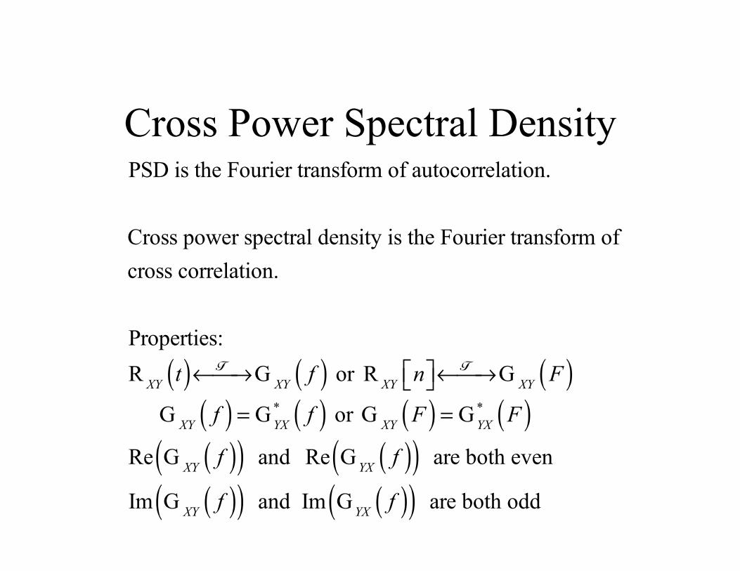
Cross Power Spectral Density

PSD is the Fourier transform of autocorrelation.

Cross power spectral density is the Fourier transform of cross correlation.

Properties:R XY t( ) F← →⎯ G XY f( ) or R XY n⎡⎣ ⎤⎦

F← →⎯ G XY F( ) G XY f( ) = GYX

* f( ) or G XY F( ) = GYX* F( )

Re G XY f( )( ) and Re GYX f( )( ) are both even

Im G XY f( )( ) and Im GYX f( )( ) are both odd


Two Random Signals


Crosscorrelation and CPSD of Two Random

Signals


Two Random Signals Plus Narrowband Interference


Crosscorrelation and CPSD of Two Random Signals Plus Narrowband Interference

Measurement of Power Spectral Density

A natural idea for estimating the PSD of an ergodic stochasticCT process is to start with the definition,

G X f( ) = limT→∞

EF XT t( )( ) 2

T

⎛

⎝

⎜⎜⎜

⎞

⎠

⎟⎟⎟

and just not take the limit.

G X f( ) =F XT t( )( ) 2

TUnfortunately this approach yields an estimate whose variancedoes not decrease with increasing time T .

Measurement of Power Spectral Density

Another approach to estimating PSD is to first estimateautocorrelation and then Fourier transform that estimate.We can estimate autocorrelation from

R X τ( ) = 1T − τ

X t( )X t + τ( )dt0

T −τ

∫ , 0 ≤ τ << T

This estimate does improve with increasing time T .

Later we will see another, even better, technique for estimating PSD and CPSD.

power spectral density -...

Documents