power system laboratory manual€¦ · steady state performance of a transmission line objectives:...

Power System Laboratory Manual

B.Tech, 4th Year, 7th Semester Electrical Engineering Department

Indira Gandhi Institute of Technology Sarang ,Dhenkanal-759146, Odisha

L.N Tripathy @ Electrical Engineering Department-2017

EE /IGIT/2016/ Faculty : L.N Tripathy

Indira Gandhi Institute of Technology, Sarang, Dhenkanal B.Tech, 4th Year, 7th Semester, Electrical Engineering Department

Power System Laboratory

Group A: HARDWARE BASED

1. To plot the Inverse Definite Minimum Time (IDMT) characteristic of an over-current relay with different plug setting multiplier (PSM) and time setting multipliers (TSM).

2. To study the operating principle and characteristics of a biased differential relay with different percentages of biasing setting.

3. Steady State performance of a Transmission Line Objectives: (a) To determine A, B, C, D parameters, Characteristic Impedance and Propagation

Constant of an artificial transmission line. (b) To determine the voltage profile of a Transmission Line

(i) Without Shunt Compensation (ii) With Shunt Compensation.

(c) To determine the reactive power required for zero voltage regulation at different loads (d) To Study the Ferranti Effect of Long Transmission Line.

4. Voltage Control Using STATIC VAR Compensator 5. Study of Performance of the Buchholz Relay used for Protection of Transformer

Group B : SIMULATION BASED (MATLAB OR ANY OTHER SOFTWARE)

1. To formulate the Y-Bus matrix for standard Electrical Network. 2. To compute voltage, current, power factor and regulation at the receiving end of a three

phase Transmission line (Pi Model) when the voltage and power at the sending end are given and further calculate the efficiency of the Transmission Line at that particular Load.

3. Simulation of symmetrical and unsymmetrical faults in a given Transmission line connected to power network and study of variation of parameters such as Fault type, Fault resistance, Fault Location and Source Impedance on current & voltage magnitude and phase measured at sending end.

TEXT BOOKS: 1. Hadi Sadat- Power System Analysis – TMH 2. T. K. Nagsarkar and M. S. Sukhija - Power System Analysis – Oxford University

Indira Gandhi Institute of Technology Electrical Engineering Department

B.E , IV Year(7th Semester), Electrical Engineering Department Power System Lab

Certificate

This is to Certify that Mr/Ms ---------------------------------------------

---------- University Regd. No ----------------------------------of

B.Tech 7th Semester Electrical Engineering Department has

completed all experiments prescribed by the Institute as per

requirement of B.Tech[Electrical ] Engineering Degree of Biju

Patnayak University of Technology, Rourkela for the Academic

Year -----

Faculty Signature Head of Department Date:-


Index Sr.No Name of the Experiments Date Grade Faculty

Signature 1

2

3

4

5

6

7

8

9

10

Name of Student:- Group:- Roll No :- University Regd. No

1 | P a g e P S P / L . N T r i p a t h y

Indira Gandhi Institute of Technology, Sarang, Dhenkanal

B.Tech, 4th Year, 7th Semester, Electrical Engineering Department Experiment No. Date:- Aim:- Development of a Matlab program showing the variation real power through a line w.r.t load angle () and reactive power variation through a line w.r.t variation in terminal voltage of the line. Example:-

Two Voltage sources V1=120<-50 V and V2 = 100<00 V are connected by a short line of

Impedance Z= 1+j7 . Write a Matlab program such that the phase angle of source- 1 is

changed from its initial value by 300 in a step of 50. Voltage magnitude of two sources

and Voltage phase angle of sources-2 is kept constant.

Q1.

(a) Tabulate the real power at Source-1 (P1) and Real Power at Source-2(P2)and

Power Loss in the Line( PL) for different values of Source-1 voltage phase angle

().

(b) Plot P1, P2 and PL w.r.t Source-1 voltage phase angle ().

(c) Plot Reactive Power at Source-1(Q1) and Reactive Power at Source-2(Q2) w.r.t

(d) Gives your comments on the result in part(c)

Q2. Plot Reactive power at Source-1 (Q1) and Reactive Power at Source-2(Q2) and

Reactive Power Loss in the Line( QL) for different values of Source-1 voltage magnitude

while load angles of both sources and source-2 voltage magnitude are remained constant.

Comment on the above results

Group No.:- Student Name:- Roll No

2 | P a g e P S P / L . N T r i p a t h y

Mathematical Analysis and Related Formula

0 00

12

0 00

21

* 012 1 12

* 021 21

12 21

120 5 100 0 3.135 110.021 7

100 0 100 5 3.135 69.981 7

376.2 105.02 97.5 363.3

2 313.5 69.98 107.3 294.59.8 68.8

ReL

Ij

Ij

S V I W j Var

S V I W j VarLine Loss S S S W j Var

al Power Los

2 2

122 2

12

( ) 1 (3.135) 9.8

Re ( ) 7 (3.135) 68.8

L

L

s P R I W

active Power Loss Q X I Var

References:-1. Power System Analysis, Hadi Saadat, TATA McGRAW- HILL, Edition.2004, Page no:26-30

3 | P a g e / P S P / L . N T r i p a t h y


Experiment No. Date:-

1. Aim : Steady State performance of a Transmission Line Objectives: (a) To determine A, B, C, D parameters, Characteristic Impedance and Propagation

Constant of an artificial transmission line. (b) To determine the voltage profile of a Transmission Line

(i) Without Shunt Compensation (ii) With Shunt Compensation.

(c) To determine the reactive power required for zero voltage regulation at different loads (d) To Study the Ferranti Effect of Long Transmission Line.

Motivation:

Transmission line are used to transfer bulk amount of power from one place to other in Electrical system. The availability of well developed high capacity system of transmission line makes it technically and economically feasible to transmit block amount of power over large distance.

The performance characteristic of transmission line are important from the point of view of making analytical studies of the system , e.g power flow, voltage regulation ,steady state and transient stability etc.

Theory :

A Transmission line has four parameters (i) Resistance (ii) Inductance (iii) Capacitance and (iv) Conductance. Where (i) and (ii) makes up the series impedance of the line , (iii) &(iv) determine shunt admittance. Shunt conductance are generally neglected in power Transmission line when calculating voltage and current.

The classification of Transmission lines according to length depend upon what approximations are justified in treating the parameters of the lines. The Transmission lines are classified as

(a) Short Transmission line : These lines are roughly 80 km long . For short transmission line the total capacitive susceptance is so small that it may be neglected(Figure-1).

(b) Medium Line : Medium lines are roughly between 80 240 km long. The shunt admittance, generally pure capacitance is included in the equivalent circuit of the line.


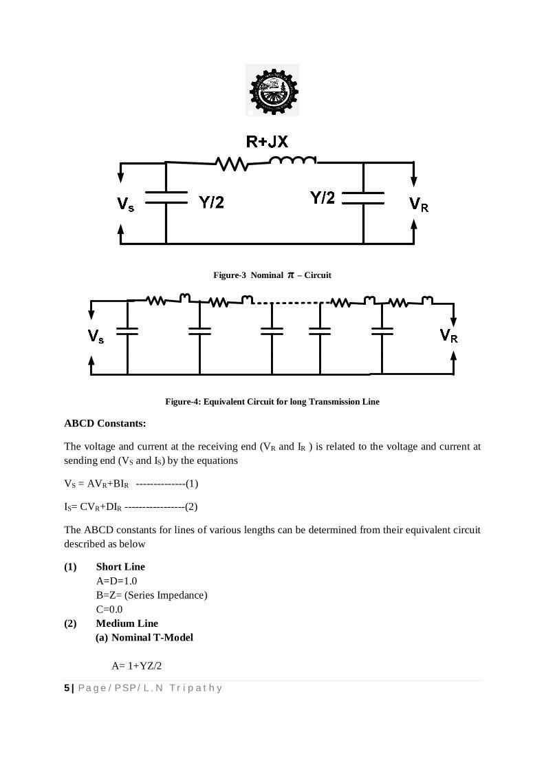
If all the shunt admittance is lumped at the middle of the circuit representing the line , the circuit is called Nominal-T(Figure-2). In the Nominal- ߨ circuit the shunt admittance is divided into two equal parts placed at sending and receiving end of the line(Figure-3). Long Line: Lines more than about 240km long require calculation in terms of distributed constant if a high degree of accuracy is required. An equivalent circuit representing for such line are shown in figure-4 Let Z= Series impedance per unit length per phase y= Shunt Admittance per unit length per phase l = length of the line Y=yl.

VRVs

Z=R+jX

R X

Figure-1 : Equivalent Circuit of Short Transmission Line

Figure-2 Nominal T- Circuit


Figure-3 Nominal π – Circuit

Figure-4: Equivalent Circuit for long Transmission Line

ABCD Constants:

The voltage and current at the receiving end (VR and IR ) is related to the voltage and current at sending end (VS and IS) by the equations

VS = AVR+BIR --------------(1)

IS= CVR+DIR -----------------(2)

The ABCD constants for lines of various lengths can be determined from their equivalent circuit described as below

(1) Short Line A=D=1.0 B=Z= (Series Impedance) C=0.0

(2) Medium Line (a) Nominal T-Model

A= 1+YZ/2


B= Z+YZ2/4 C=Y D=1+YZ/2

(b) Nominal π-Model A= 1+YZ/2 B=Z C=Y+ZY2/4 D=1+YZ/2

The characteristic Impedance(ZC) of a Transmission line is given by

CZZY

---------------------(3)

The Propagation Constant (ϒ) of the line is given by

YZ --------------------(4)

Line on No-Load:

A long transmission line with no load at receiving end gives a voltage rise at the receiving end. This effect is commonly known as Ferranti effect. The reason for these phenomena is the negative voltage drop caused by line charging current. This effect can be neutralized if an Inductive load is connected at the receiving end.

The voltage drop caused at the receiving end of the line because of inductive load as well as voltage rise because of the line charging current at light load or no load , can be neutralized by choosing proper static capacitor /synchronous capacitor or shunt reactor at receiving end . Such compensation can give zero voltage regulation.

Pre Experimental Quiz:

1. What are the various parameters of the Transmission line 2. Differentiate between Short, Medium and long line 3. What is the physical significance of attenuation constant of a long Transmission line 4. What is the difference between nominal –π and equivalent π network of a transmission

line. 5. What do you understand the series and shunt compensation of the line ? Where are these

used.


6. Why Transmission Lines are Transposed? 7. What is the effect of Earth on the capacitance of the Transmission Line 8. Does Spacing of the line affect the line parameters ? What other physical factors effect

the line Parameters

Equipments:- Transmission Line simulator

Procedure:

1. Determination of ABCD Constants: (a) Connect the apparatus as shown in figure-5. Measure Is with receiving end open-

circuited (IR=0), Then ZSO=VS/IS=A/C (b) Short circuit the receiving end (VR=0) and increase the VS gradually such that IS does

not exceed the rated value of current. Measure VS, IS. Then ZSS=VS/IS=B/D

(c) Open circuit the sending end(IS=0), apply voltage from receiving end Then ZRO= VR/IR=D/C

(d) Short circuit the sending end(VS=0). Increase the voltage at receiving end gradually such that IR does not exceed the rated values of the current. Measure VR,IR. Then ZRS= VR/IR=B/A.

(e) From the above result , calculate

( )SO

RO RS

ZAZ Z

, Also calculate other constants

(f) From the above test results , calculate ZC & γ

2. Shunt Reactor: Connect an inductive load at receiving end such that it completely compensate the voltage rise due to line capacitance i.e the voltage at two ends of the line are equal

3. Voltage Profile: (a) With full load at the receiving end , measure the voltage at 0,1/4th,1/2,3/4th and full

length of the line. Plot voltage versus line length. (b) Use proper shunt compensation, measure the voltage again. Plot the voltage versus

line length.

4. Zero Regulation


With full load ,3/4th full load,1/2 load ,1/4th load and no load (inductive) at receiving end ,determine the values of shunt capacitor C, such that VS=VR. The connection diagram is shown in figure-6

Figure-5, Open Circuit and Short Circuit Test on Transmission Line

Figure-6, Zero Voltage Test on Transmission Line


DATA SHEET:

1. ABCD Constants:

VS IS ZSO Remarks

VS IS ZSS Remarks

VR IR ZRO Remarks

VR IR ZSR Remarks

2. Shunt Reactor Compensation:

VS VR=VS IR IS W CosΦ Compensating XL Reactance

3. Voltage Profile:

V0 At Sending end

V1 At .25 Distance

V2 At .50 Distance

V3 At 0.75 Distance

V4 At 1.0 Distance

Remark

Without Compensation

With Compensation


4. Shunt Compensation for Zero voltage Regulation:

VS I’R IR VR=VS C W CosΦ Remark

1 Full Load

2

3

4

5

Data Processing and Analysis:

For each of the above studies, comment on the observed values(Measurements) and calculated values of voltages, currents , power factors, shunt reactor, static capacitors etc.

Post Experimental Questions:

1. Comment on the effect of shunt compensation of a Transmission Line 2. What are the various material used for Transmission Line conductor 3. Why are the bundle conductors are used EHV Transmission Line 4. What can be benefit of automatic control for shunt compensation 5. What do you understand by Surge Impedance Loading of a Transmission Line 6. What is understood by a half-wavelength Transmission Line

References:

1. Zaborsky, ‘Transmission Line’ 2. W.D Stevenson, ‘Elements of Power System Analysis’ 3. O.I Elgerd, ’Electric Energy System Theory’, McGraw Hill Publisher 4. Nagrath & Kothari, ‘Power System Analysis’ 5. B.M Weedy, ‘Power System’


Indira Gandhi Institute of Technology,

Electrical Engineering Department B.E , IV Year(7th Semester), Electrical Engineering Department

Power System Lab


Indira Gandhi Institute of Technology

Electrical Engineering Department B.E , IV Year(7th Semester), Electrical Engineering Department

Power System Lab

Experiment No Date: Aim:-Write the Matlab program to form the Y Bus of the Electrical network with line data given below and show the results ? Line Data:

From Bus

To Bus

Line Resistance(R)

Line Reactance(X)

Shunt Susceptance(B/2)

1 2 0.05 0.15 0.000

1 3 0.10 0.30 0.000

2 3 0.15 0.45 0.000

2 4 0.10 0.30 0.000

3 4 0.05 0.15 0.000

Q. 1 . Write some specific characteristic of Y- Bus matrix Q 2. Why Y-Bus matrix is essential for load flow analysis and not Z -Bus matrix Q. 3. A Electrical Network comprises of 20 buses and 30 Transmission line.

(a) What is the size of Y-Bus Matrix (b) In the above Y-Bus Matrix how many elements will be zero and how many

elements will be non-zero (c) Explain the sparsity of a matrix.

Group No:- Student Name Roll No



Experiment No. Date:- Aim:- Simulate a Transmission line model given below with single phase to ground fault having fault resistance of 0.001 ohm and ground resistance of 0.001 ohm with following parameters. The total simulation time is 1.0 second and fault is incepted at 0.7 second and continued till 1.0 second. Source Parameters:- Source-1

Phase to Phase Vrms =400kv, Phase Angle = 100 , Frequency =50 Hz, Source resistance

= 0.8929 Ohm, Source Inductance = 16.58 mH

Source-2

Phase to Phase Vrms =400kv, Phase Angle = 00 , Frequency =50 HZ, Source resistance

= 0.8929 Ohm,Source Inductance = 16.58 mH

Transmission Line Parameters:-

R = 0.01273 ohm/km,L = 0.9337mH/km,C =1274nF, Length of line = 200 km

(a) Plot line current, Line voltage & power for different types of fault[LL, LLG,

LLLG with different fault inception angle[00, 900] when fault distance is 100km

from source-1

(b) For A-phase to ground fault with above fault resistance , Ground resistance and

fault distance from source-1, list the different harmonics components relative to

fundamental and find the corresponding THD during the fault interval (0.7 to 1.0

second) using FFT analysis.

(c) Comment on the above results

Group No.:- Students Name:- Roll No

17 | P a g e / P S P / L N T r i p a t h y

Indira Gandhi Institute of Technology, Sarang, Dhenkanal

B.Tech, 4th Year, 7th Semester, Electrical Engineering Department Aim:- In the below RLC circuit , R= 1.4 ohm, L= 2H, and C=0.3 F .The initial inductor Current is zero, initial capacitor voltage is 0.5 V. A step voltage of 1 V is applied at t=0. Plot the i(t) and v(t) graph over the range 0<t<15 sec. Also plot the current versus capacitor voltage and energy stored in capacitor versus time. Write the Matlab program for getting the graph for above problem and attached the figures Experiment No. Date:- Group No.:- Student Name:- Roll No




OBJECTIVE: - Steady State analysis of given Power System using Newton-Raphson method of Load Flow study.

System Data: - For 7-bus system

Line Data:

Sl. No. 1 (From bus)

2 (To bus)

3 (Line impedance)

(R + jX)

4 Line charging admittance

(b_l)/2

5 tap ratio

1 1 2 0.0000+0.1000j 0.000j 1.06

2 6 2 0.0175+0.0628j 0.030j 1+0j

3 6 5 0.0777+0.2013j 0.025j 1+0j

4 2 5 0.0573+0.158j 0.020j 1+0j

5 2 4 0.0607+0.171j 0.020j 1+0j

6 2 3 0.0431+0.14j 0.015j 1+0j

7 5 4 0.011+0.028j 0.010j 1+0j

8 4 3 0.0810+0.2065j

0.025j 1+0j

9 6 7 0.0000+0.1000j

0.010j 1.04

Bus Data

Sl. No.

1 2 3 4 5 6 7 8 9 A B C D E

1 1 0 1.06 1.00 0.0 0+0j 0.0+0.0j 1.05 -10.0 0.0 1 0 0 0.3

2 2 2 1.00 1.00 0.0 0+0j 0.0+0.0j 0.00 0.00 0.0 1 0 0 0.4

3 3 2 1.00 1.00 0.0 0+0j 0.2+0.1j 0.00 0.00 0.0 1 0 0 0.3


4 4 2 1.00 1.00 0.0 0+0j 0.4+0.05j 0.00 0.00 0.0 1 0 0 0.0

5 5 2 1.00 1.00 0.0 0+0j 0.45+0.1j 0.00 0.00 0.0 1 0 0 0.0

6 6 2 1.00 1.00 0.0 0+0j 0.6+0.1j 0.00 0.00 0.01 1 0 0 0.0

7 7 1 1.00 1.00 0.0 0.4+0j 0.0+0.0j 10.0 -10.0 0.0 1 0 0 0.0

*The column wise description is as follows: 1 -- Bus Number. 2 -- Type of Bus, 0 == slack, 1 == PV, 2 == PQ. 3 -- Initial Choice for Voltage (V) 4 -- Nominal Bus Voltage (V_n) 5 -- Initial Choice for Angle (A) 6 -- Generation Specification (P_g + jQ_g) 7 -- Nominal Load Specification (P_dn + jQ_dn) 8 -- Reactive Generation Maximum (Q_g^max) 9 -- Reactive Generation Minimum (Q_g^min) A -- Bus Shunt Susceptance (b_sh) B -- Constant Power Load Coefficient (C_p) C -- Constant Current Load Coefficient (C_c) D -- Constant Impedance Load Coefficient (C_i) E -- Generator participation factor (alp)

THEORY:- Newton-Raphson is an iterative method for solving non-linear problems. It starts with an initial guess and then makes use of the Taylor series expansion and the approximation for the solution by the first order gradient (derivative).

Neglecting the higher order terms we get

This being an iterative scheme;

The process is repeated till a convergence criterion is met. Generally the first order gradient is called the Jacobian.

푓(푥) = 푐

푓(푥푘 + 훥푥) = 푓(푥푘) + ∇푓Δ푥 +훻2푓

2!Δ푥2 +⋯ = 푐

Δ푥 = ∇푓−1[푐 − 푓(푥푘)]


The convergence criteria is generally

– max(abs(delta x)) < a specified tolerance – max(abs(mismatch)) < a specified tolerance

In Power Flow context, we have P and Q equations to be solved for Bus Voltage and Angle (Polar co-ordinates).

For Voltage dependent load,

Similar expression for Qd

i.

For Voltage dependent Q limits,

The Voltage dependent Q limits are to be handled on lines similar

– Normal Q limits when not violated. – Voltage dependent load when violated.

Result analysis :

For the 7 bus system, perform one iteration for NRLF. The one iteration in NRLF involves computation of Jacobian and the updated bus voltages and angles for that iteration. Compare the results with those with the program executions. Find the following parameters: a) Power flow in all lines b) Power loss in all lines (active, reactive both)

푃푖 = 푉푖2푟푒푎푙(푌푖푖) + 푉푖푉푗푗≠푖

[cos 훿푗 − 훿푖 푟푒푎푙 푌푗푖 − sin 훿푗 − 훿푖 푖푚푎푔 푌푗푖 ]

푄푖 = −푉푖2푖푚푎푔(푌푖푖) + 푉푖푉푗푗≠푖

[sin 훿푖 − 훿푗 푟푒푎푙 푌푗푖 − cos 훿푖 − 훿푗 푖푚푎푔 푌푗푖 ]


c) Total loop loss

Further analysis:

Check the effect of the following on convergence: – PV bus Q limit violations, – Load increase (Bus no. 2 and 3), – line R/X ratio(series comp, 30% compensation), – Gen rescheduling (loads fixed), – PV bus voltage changes (Bus 7-Change voltage to 1.06 p.u.), – Addition/removal of voltage control at a bus. – Effect of change in slack bus position (Take 7 as slack bus).




Experiment No:- Date:- Inverse Definite Minimum Time [IDMT] Characteristic of Over Current and Earth fault Relay Motivation

The protective Relaying which respond to a rise in current flowing through the protected element over a pre-determined value is called Over Current Protection and the Relay used for this purpose are known as Over Current Relay. Earth fault Relay can be provided with normal Over Current Relay. If the minimum earth faults current in magnitude is more than the pre-set value then the earth fault relay will operate otherwise the earth fault relay does not operate. The design of a comprehensive protection scheme in power system requires the detailed study of time-current characteristics of various relay used in the scheme. Thus it is necessary to obtain the operating time-current characteristic of these relays Objective

(i) To obtain the IDMT characteristic of Induction type Over Current relay (ii) To obtain the IDMT characteristic of Induction type Earth fault relay

Theory

The Induction over current relay works on induction principle. The moving system consists of an aluminum disc fixed on a vertical shaft and rotating on two jewelled bearings, between two poles of an electromagnet and a damping magnet. The winding of the electromagnet is generally provided with seven taps, which are brought on to the front panel, and required tap is selected by a push-in-type plug. The pick up current setting can be varied by the use of such plug multiplier setting. The pick up current value of earth fault relay are normally quite low. The operating time of all over current relays tends to become asymptotic to a definite minimum value with the increase in the value of current. This is an inherent property of the electromagnetic relay due to saturation of the magnetic circuit. By varying the point of saturation, different characteristic can be obtained and those are

(a) Definite Time (b) Inverse Definite Minimum Time(IDMT) (c) Very Inverse


(d) Extremely Inverse The torque of these relays is proportional to φ1 φ2Sinα , where, φ1 and φ2 are the two fluxes and α is angle between them. Where both the fluxes are produced by same quantity ( Singe Quantity relays) as in the case of current or voltage operated , the torque is proportional to I2 , the coil current below saturation or T = KI2 . If core made to saturate at a very early stage with the result that by increasing I, K decreases so that the time of operation remain the same over the working range, the time-current characteristic obtain is known as Definite Time characteristic . If the core is made to saturate at later stage , the characteristic obtain is known as IDMT. The time current characteristic is inverse over some range and then after saturation assumes the definite time form. In order to ensure selectivity, it is essential that the time of operation of relay should be depended on severity of the fault in such a way that more severe the fault, less is the time to operate, this being called Inverse-time characteristic. This will also ensure that the relay shall not operate under normal over load condition of short duration

It is essential also that there shall be a definite minimum time of operation, which can be adjusted to suit the requirement of particular installation. At low value of operating current, the shape of the curve is determined by the effect of the restraining force of the control spring, while at high value the effect of saturation predominates. Different time setting can be obtained by moving a knurled clamping screw along a calibrated scale graduated from 0.1 to 1.0 in the step of 0.05. This arrangement is called Time multiplier setting and will vary the travel of the disc required to close the contact. This will shift the time-current characteristic of the relay parallel to itself. By delaying the saturation point to further, the time current characteristic called Very Inverse and Extremely Inverse can be obtained Pre-Experimental Quiz

(1) What do you understand by (a) Primary Relay (b) Secondary Relay (c) Auxiliary Relay ? (2) What do you understand by (a) Single quantity Relay (b) Double or Multi- Quantity relay ? (3) What are the types of Over current and earth fault relay ? (4) Can the over current and earth fault relay be actuated by both A.C and D.C ? (5) What is meant by Pick-up current, Drop out current and Drop out ratio? (6) Where do you connect over current and earth fault relay ? (7) What is meant by (a) Sensitivity and (b) Selectivity of relay ?

Materials and Equipments CDG 11 over current relay, Earth fault relay, current transformer, 3 phase contactor, single phase load, Digital timer and Ammeter.


Procedure:- (1) Over current Relay

(a) Study the construction part of the relay and identify the various parts (b) Connect as per the circuit (c) Set the pick-up value of current at 100% full load current by inserting the plug in

the groove. (d) Set the time multiplier setting (TMS) initially at 1.0 (e) Adjust the load current to about 1.3 times the full load current by shorting the

switch K . Open the switch K to permit this adjusted current to flow through the relay via current transformer and record the time taken for this over load condition.

(f) Vary the value of load current in step and record the time taken for operation of the relay in each case with help of timer.

(g) Repeat the step (e) and (f) for TMS value of 0.2, 0.4, 0.6 and 0.8. (h) Repeat the above experiment with different pick-up current values using the plug

setting Bridge.

(2) Earth Fault Relay

(a) Study the construction part of the relay and identify the various parts (b) Connect as per the figure replacing the over current relay by earth fault relay (c) The pick-up value of the current is set to Full load current using plug setting Bridge (d) Set the TMS to 1.0 (e) Vary the load current in different steps as in part (1) and record the operating

current value and the time of operation in each case. (f) Repeat the step (e) for different TMS value as in over current experiment. (g) Repeat the above experiment with different pick-up current values( Using the

plug setting bridge, pick-up current can be varied) Data Sheet: (1) Type of Relay : Pick up Current ( Plug Set) = Sr. No

Current In Amp.

Plug Setting Multiplier (PSM)

Operating Time in Secs for TMS of

0.2 0.4 0.6 0.8 1.0 1


2

3

4

5

6

Data Processing and Analysis

(a) Plot the operating time versus the multiple of plug setting value for different TMS on the same graph for over current relay

(b) Plot on a log-log sheet operating time versus the multiple of plug setting value for different TMS on the same graph for over current relay

(c) Observe the Inverse nature of the characteristic as well as the definite minimum time required for the operation of the relay in either case if possible

Post Experimental Quiz

(1) Do you like to add directional feature for over current protection ? (2) Can the over current and earth fault relay made to operate instantaneously and

how ? (3) Why the relay disc is not normally circular ? (4) What are the equation of IDMT, very inverse, extremely inverse over current

relay ? (5) When do you use negative phase sequence filter

Reference:

(1) A.R Van C. Warrington ‘Protective Relays , There theory & Practice Volume I and II’ , Chapman & Hall

(2) C.R Mason , ‘ Art and Science of Protective Relays’. (3) B. Ravindranath and M. Chander, ‘ Power System Protection and Switch Gear’. (4) Y.G Paithankar, S.R Bhide, ‘Fundamental of Power System Protection’, PHI


IDMT Relay Diagram

Figure 1


Connection Diagram




Experiment No :- Date:- Principle of Circulating Current differential Relaying Motivation

Fault and abnormal conditions are inevitable in power system. In order to provide normal operation of the power system and consumer units, it is necessary to detect and isolate the fault from the healthy circuit in the shortest possible time, thus restoring the normal operating condition. Protective Relaying employed for such task should have qualities of Selectivity, Speed of Operation, Sensitivity and Reliability. Differential protection fulfils these requirements to large extend. The differential scheme is particularly suitable for alternator, Transformer, Transmission line, feeder etc. The main requirement of differential protection scheme is that the Current Transformers used in this scheme should be properly matched. In case such a matched pair is not available , there would be an imbalance secondary current and this should be pre-determined in order to adjust the relay setting. The relay should not operate for this imbalance current. Objectives

(a) To determine the imbalances in Current Transformers in the normal operating range

(b) To study the circulating current differential scheme. Theory

Differential protection is a unit protection scheme which protect a particular equipment for particular fault. For protection of generators, normally unbiased differential relays are used.

The differential relay senses the vector difference between incoming and outgoing current of the equipments to be protected. Figure given below explain principle of differential relay.

During healthy condition, the incoming current I1 and outgoing current I2 will be equal. So the CT secondary current will be equals and no current will flow through the relay coil.. Similar is the case for external fault at F1 . In this case incoming and outing current obviously will be very high , however they will be equal in magnitude and phase.


The current transformers, if faithfully transform the current, then the secondary current i1 and i2 will be equal and there will be no current in the relay coil. When there is an internal fault at ‘f’ , the currents i1 and i2 will not be equal and hence differential current (i1-i2) will flow through the relay coil. If this current is higher than the pick-up setting of the relay, it will operate , tripping the Circuit Breaker and thus isolating the faulty apparatus from the source. Figure(1)

Requirement of Differential Protection:-

(1) The differential protection scheme should be sensitive for in-zone fault and should be stable against external fault

(2) The C.T s should be connected with proper polarity as shown in figure, otherwise the sum of the current (i1 + i2 ) will flow through the differential relay and hence the relay will operate even in healthy condition of the equipment to be protected.

(3) For ensuring the stability of differential protection scheme against external fault, the CTs should be identical w.r.t to their saturation characteristic. The knee point voltage of CTs should be high.

Pre-Experimental Quiz

(1) What do you understand by sensitivity of Relay? (2) What are likely consequences if faults are not cleared fast? (3) Why do the current transformer exhibit non identical characteristic? (4) What are the problems can be caused due to the non-identical characteristic of

CTs (5) What is magnetic inrush current in transformer and what is its consequences ? (6) Why this scheme is not normally used for protection of transmission line? (7) Can a current balance protection scheme be used for protection of busbar ?


Procedure:- (Figure 2)

(1) See that switch S1 and S2 are open and autotransformer supply zero voltage. Now press the start button . Slowly apply the supply voltage through the autotransformer in step of 25 volt and note the reading of ammeter A1, A2 and A3. This is the normal condition where ammeter A1 , A2 will show the same magnitude of current and ammeter A3 will show zero reading. The relay will not operate.

(2) Again reduce the supply voltage to zero by autotransformer. Close the switch S2, increase the supply voltage in step of 25V and note the reading of ammeter A1, A2 and A3. This is the condition of external fault where ammeter A1 and A2 will show same ( but higher than the former case) magnitude of current. The relay will not operate.

(3) Again reduce the supply voltage. Open the switch S2 and close switch S1, increase the supply voltage in step of 25V and note the reading of Ammeter A1,A2 and A3. Observe the operation of relay and tripping of circuit breaker. This is the condition of internal fault where the current shown by ammeters A1 and A2 will differ by a value shown by ammeter A3.

The relay operates after the supply voltage is sufficient to pass more than the pick-up value of the current through the relay coil. Reverse the polarity of any CT. So the CTs are now connected with incorrect polarity. The current (i1 +i2) will flow through the relay coil. Therefore relay will mal operate in normal condition.

Figure 2

Data Processing and Analysis. Actual Reading


Sr. No

Type of Operation

Supply Voltage

in Volt.

Incoming Current

Iin in Amp.

Out going Current

Iout in Amp

Diverted Current

Idiv in Amp

Relay Current

In Amp.

Remark

1 Normal 2 Internal

fault

3 Internal fault

4 Internal fault

5 Internal fault

6 Internal fault

7 Internal fault

8 CT polarity

Reversed

Post Experimental Quiz:-

(1) Why the differential Relay operate only for Internal fault but remain insensitive to external fault ?

(2) Why the relay operate when one of the CT polarity is reversed ? (3) What do you mean by basic setting and biased setting of differential relay ? (4) Explain why biased differential relay is required for Transformer Protection ? (5) What are the Applications of differential relay ? (6) Write the technical specification of Differential Relay ?

Reference:

(1) A.R Van C. Warrington ‘Protective Relays , There theory & Practice Volume I and II’ , Chapman & Hall

(2) C.R Mason , ‘ Art and Science of Protective Relays’. (3) B. Ravindranath and M. Chander, ‘ Power System Protection and Switch Gear’. (4) Y.G Paithankar, S.R Bhide, ‘Fundamental of Power System Protection’, PHI


power system laboratory manual€¦ · steady state performance of a transmission line objectives:...

Documents