ppa 723: managerial economics lecture 2: demand and supply

PPA 723: Managerial Economics

Lecture 2:

Demand and Supply

Managerial Economics, Lecture 2: Demand and Supply

OutlineDemand

Demand CurvesMovement Along vs. Shift In Demand CurveExamples

SupplySupply CurvesMovement Along vs. Shift in Supply CurveExamples


Demand Curve

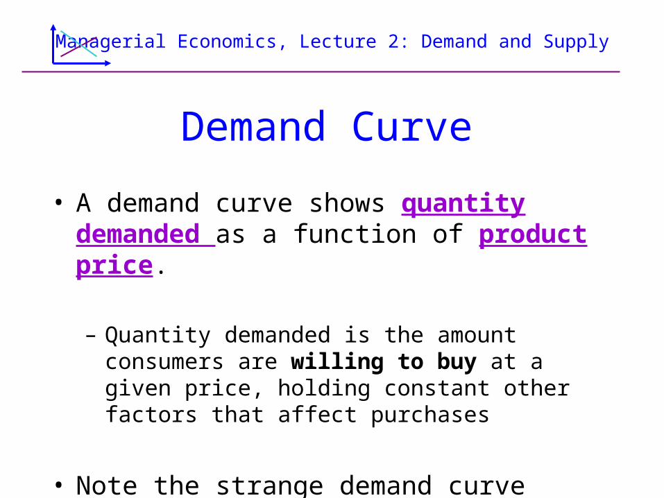
• A demand curve shows quantity demanded as a function of product price.

– Quantity demanded is the amount consumers are willing to buy at a given price, holding constant other factors that affect purchases

• Note the strange demand curve convention: price is on the vertical axis


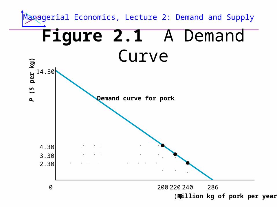
Figure 2.1 A Demand Curve

200 220

Demand curve for pork

240 286

Q (Million kg of pork per year)

0

2.303.30

4.30

14.30

P (

$ p

er k

g)


Effect of a Price Changes

A price change leads to movement along the demand curve.

A demand curve indicates: What happens to the quantity

demanded as the price changes, holding all other factors constant?


The Law of DemandDemand curves slope downward

A drop in price results in an increase

in quantity demanded, holding other factors constant.

This is one of the most important empirical finding in economics


Other Factors That Might Affect Demand

IncomePrices of other goods (compliments,

substitutes)PreferencesNumber of consumersInformation


Background Factors

Background factors are variables in the background of a given graph

We can only plot two variables at a time (three if we are careful) but the world is more complex than this!

So we distinguish between movement along a demand curve (caused by a change in price) and a shift in a demand curve (caused by changes in background factors)


Example: The Impact on Pork Demand

of a Rise in the Price of Beef

Beef is a substitute for pork

At a given price of pork, a rise in the price of beef causes some people to switch from beef to pork.


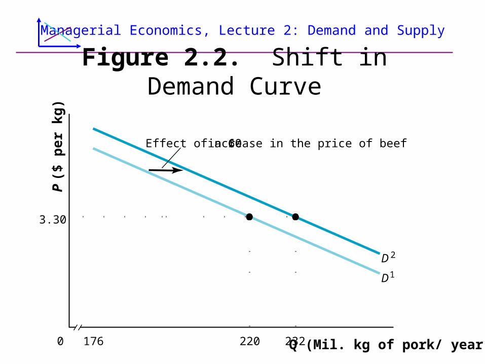
Figure 2.2. Shift in Demand Curve

220176

Effect of a 60¢ increase in the price of beef

D1

D 2

232 Q (Mil. kg of pork/ year)0

3.30

P (

$ p

er

kg

)


Demand Functions

A more general approach is to say that quantity demanded is a function of many variables, not just price.

We focus on price because it is what adjusts to make markets clear.

But sometimes we want to focus on other variables.


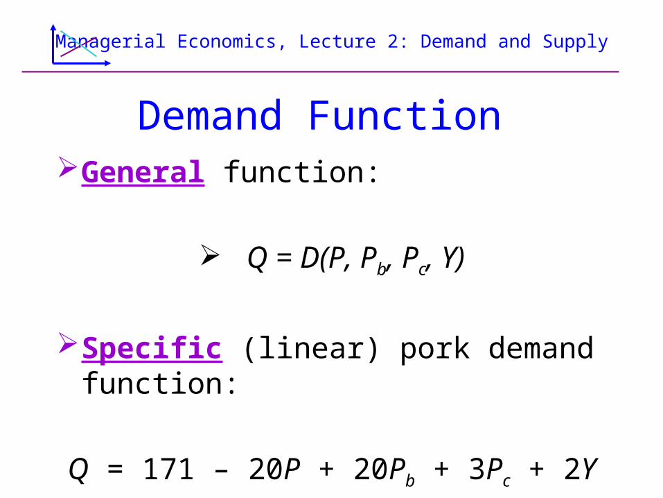
Demand Function General function:

Q = D(P, Pb, Pc, Y)

Specific (linear) pork demand function:

Q = 171 – 20P + 20Pb + 3Pc + 2Y


Other Graphs

Once we have a demand function, we can draw graphs with any two variables.

Consider, e.g., an income-consumption curve:How much do people consume (Y-axis) at different

income levels (X-axis)?Price is a background factor in this curveWe still can only plot two factors at a time!


Determining Price

One cannot determine the market price without the supply side. If we know price, can determine quantity demanded. If we know change in price, can determine movement along the

demand curve.

Demand curves are only hypothetical. They indicate what people would demand if the price were at a

certain level -- not what they actually demand. To find actual demand we must combine supply and demand,

the topic of our next class.


Example: Public Transportation

• What happens to ridership if the fare goes up?• What happens to ridership if the elderly get a

lower fare?• What happens to ridership as incomes go up?• What happens to ridership if the price of

gasoline goes up?


Example: Energy

• What happens to consumption when the price or energy goes up?

• What form does this change take? lower thermostats? more sweaters? less driving? smaller cars?

• What happens to natural gas consumption when oil prices go up?

• What happens to energy consumption with a new conservation ethic? How would you distinguish this from a price increase?


Example: Health Care

• What happens to consumption when the price goes to zero because of insurance?

• What happens to consumption of (legal) drugs as generic drugs become more available?


Example: Local Public Services

There is lots of evidence that demand is reflected in voting and in public spending.

So: • What happens to school quality when teachers'

salaries rise?• What happens to school quality when the cost of

police goes up?• What happens to school quality when the state gives

grants that lower the price of schools to city residents?


The Supply Side

The behavior of suppliers is quite different from the behavior of demanders.

But the analytical issues are similar.

Quantity supplied is the amount of a good or service that firms want to sell at a given price, holding constant other factors that affect supply.

We focus for now on firms that are small relative to the market, so they can each sell as much as they want at the market price.


Supply CurveAn increase in price of pork causes a

movement along the supply curve (holding fixed other variables that affect supply)

A supply curve answers the question:What happens to the quantity supplied

as the price changes holding all other factors constant?


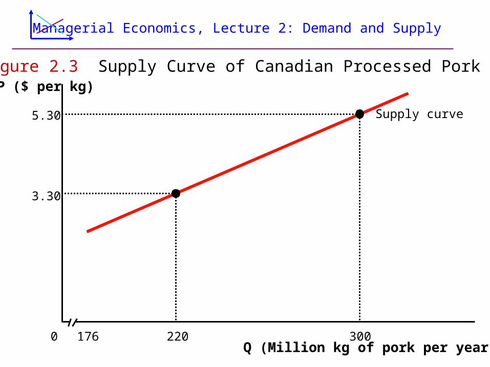
Figure 2.3 Supply Curve of Canadian Processed PorkP ($ per kg)

220176

Supply curve

300Q (Million kg of pork per year)

0

3.30

5.30


Effect of Price on Supply

Supply curve for pork is upward sloping

Increase in the price of pork leads to movement along the supply curve, resulting in larger quantity of pork supplied


Background Factors in Supply Curve

input pricestechnologynumber of firms (and conditions in other

markets)goals of the firmregulation


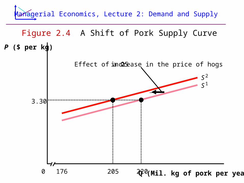
Figure 2.4 A Shift of Pork Supply Curve

P ($ per kg)

205176

Effect of a 25¢ increase in the price of hogs

S1S2

220 Q (Mil. kg of pork per year)0

3.30


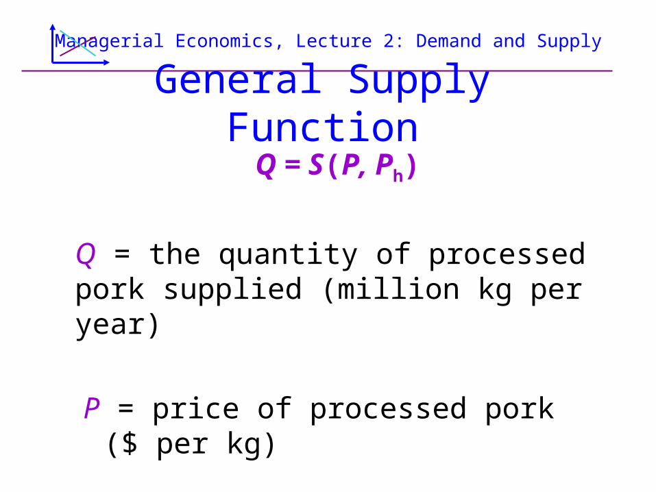
General Supply Function

Q = S(P, Ph)

Q = the quantity of processed pork supplied (million kg per year)

P = price of processed pork ($ per kg)

Ph = price of a hog ($ per kg)


Supply Curves and Market Outcomes

Supply curves, like demand curves are hypothetical.

We cannot determine what the price will be without combining supply and demand.


Summing Demand Curves

Market demand curve:

equals horizontal summation of individual demand curves

shows total quantity demanded by all demanders at each possible price


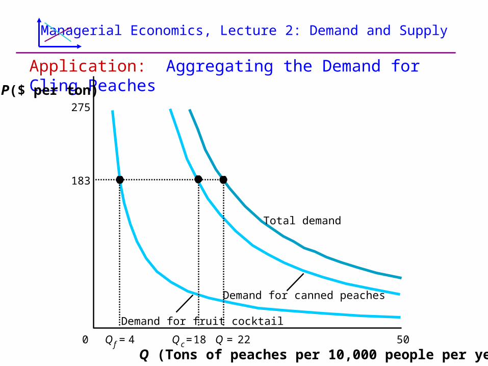
Application: Aggregating the Demand for Cling Peaches

P($ per ton)

50

Q (Tons of peaches per 10,000 people per year)0

275

183

Total demand

Demand for canned peaches

Demand for fruit cocktail

Qc = 18 Q = 22Qf = 4


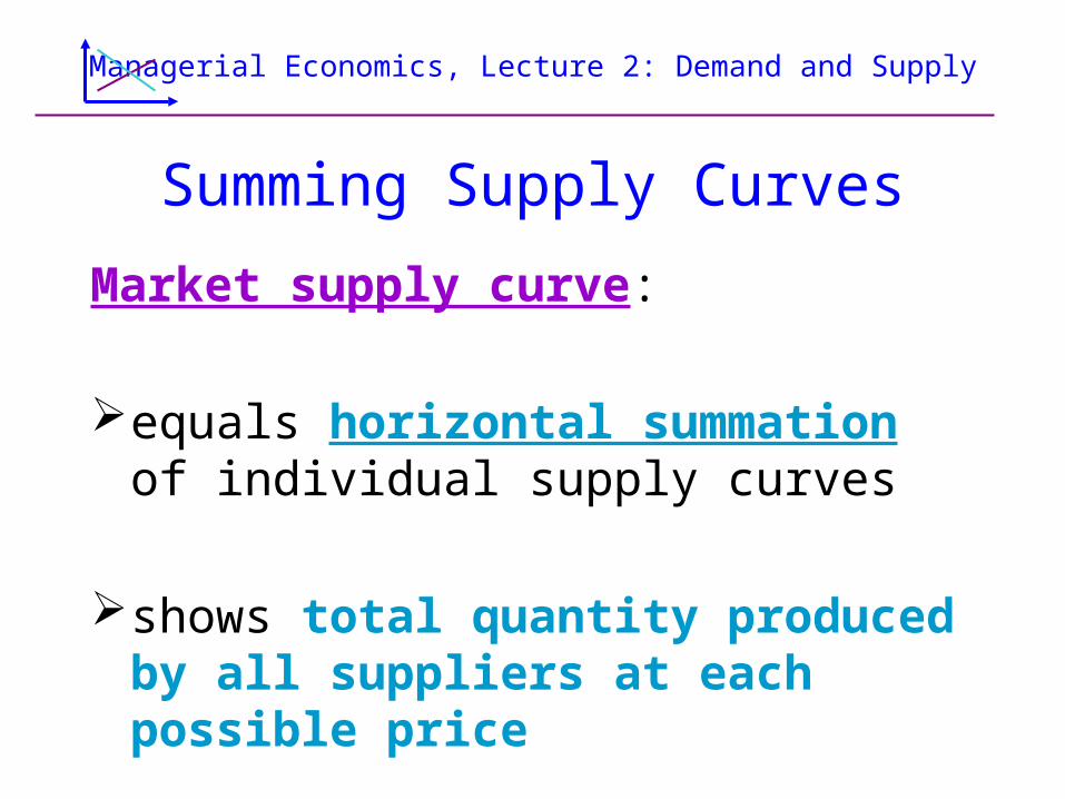
Summing Supply Curves

Market supply curve:

equals horizontal summation of individual supply curves

shows total quantity produced by all suppliers at each possible price


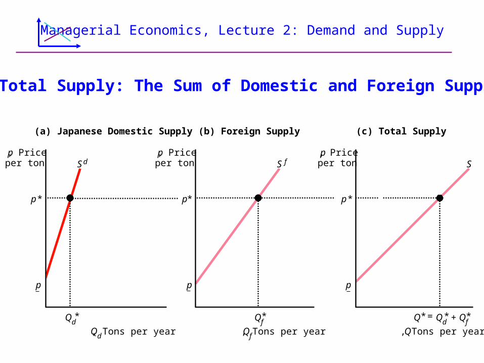
Total Supply: The Sum of Domestic and Foreign Supply

p, Priceper ton

p, Priceper ton

p, Priceper ton

Qd*

Sd

Qf* Q* = Qd

* + Qf*

Qd, Tons per year Qf, Tons per year Q, Tons per year

(a) Japanese Domestic Supply (b) Foreign Supply (c) Total Supply

p * p* p *

S S f

p p p

ppa 723: managerial economics lecture 2: demand and supply

Documents

supply demand curve

law of demand demand

supply demand functions

supply slide

economics slide

managerial economics

demand income prices

supply curve examples