PRACHT WETLAND LANDCOVER INVENTORY

Final Report

Submitted to:

Kansas State Conservation Commission

by

Kansas Applied Remote Sensing ProgramJerry L. Whistler, P.I.John Dunham, Ph.D.

August 1995

Contract No. 95-63KU Award No. 5417-0708 KARS Report No. 95-1

ii

Table of Contents

List of Figures and Tables . . . . . . . . . . . . . . . . . . . . . . . . . . . . . . . . . . . . . . . . . . . . . . . . . . . . . . iii

Acknowledgments . . . . . . . . . . . . . . . . . . . . . . . . . . . . . . . . . . . . . . . . . . . . . . . . . . . . . . . . . . . . iv

Executive Summary . . . . . . . . . . . . . . . . . . . . . . . . . . . . . . . . . . . . . . . . . . . . . . . . . . . . . . . . . . . . 1

Background . . . . . . . . . . . . . . . . . . . . . . . . . . . . . . . . . . . . . . . . . . . . . . . . . . . . . . . . . . . . . . . . 2

Introduction . . . . . . . . . . . . . . . . . . . . . . . . . . . . . . . . . . . . . . . . . . . . . . . . . . . . . . . . . . . . . . . . 4

Materials and Methods . . . . . . . . . . . . . . . . . . . . . . . . . . . . . . . . . . . . . . . . . . . . . . . . . . . . . . . . . . 4

Data Sources . . . . . . . . . . . . . . . . . . . . . . . . . . . . . . . . . . . . . . . . . . . . . . . . . . . . . . . . . . . 5

Land Use/Land Cover Classes . . . . . . . . . . . . . . . . . . . . . . . . . . . . . . . . . . . . . . . . . . . . . . 7

Field Observations . . . . . . . . . . . . . . . . . . . . . . . . . . . . . . . . . . . . . . . . . . . . . . . . . . . . . . . 9

General Interpretation Strategy and Tiling Scheme . . . . . . . . . . . . . . . . . . . . . . . . . . . . 10

Evaluation of Aerial Photography . . . . . . . . . . . . . . . . . . . . . . . . . . . . . . . . . . . . . . . . . . 11

NAPP Orthorectification . . . . . . . . . . . . . . . . . . . . . . . . . . . . . . . . . . . . . . . . . . . . . . . . . 11

ASCS Slide Rectification . . . . . . . . . . . . . . . . . . . . . . . . . . . . . . . . . . . . . . . . . . . . . . . . . 15

Photo Interpretation and Splitting the Coverages into Tiles . . . . . . . . . . . . . . . . . . . . . . 16

iii

Table of Contents (cont.)

Project Results . . . . . . . . . . . . . . . . . . . . . . . . . . . . . . . . . . . . . . . . . . . . . . . . . . . . . . . . . . . . . . . 22

Delivered Products . . . . . . . . . . . . . . . . . . . . . . . . . . . . . . . . . . . . . . . . . . . . . . . . . . . . . . 23

Polygon Attribute Documentation . . . . . . . . . . . . . . . . . . . . . . . . . . . . . . . . . . . . . . . . . . 25

Conclusions . . . . . . . . . . . . . . . . . . . . . . . . . . . . . . . . . . . . . . . . . . . . . . . . . . . . . . . . . . . . . . . 27

Bibliography . . . . . . . . . . . . . . . . . . . . . . . . . . . . . . . . . . . . . . . . . . . . . . . . . . . . . . . . . . . . . . . 29

Appendix A: Land Use/Land Cover Definitions . . . . . . . . . . . . . . . . . . . . . . . . . . . . . . . . . . . . . 30

Addendum A: Summary Acreage for Land Covers in the Pracht Wetland (1994) . . . . . . . . . . . 34

iv

Figures

Figure 1. Example of Digital Elevation Model data for the Wichita West Quadrangle . . . . . . . . 8

Figure 2. Public Land Survey overlayed on the orthorectified 1991 NAPP photography . . . . . 14

Figure 3. Public Land Survey overlayed on the rectified 1994 ASCS photography . . . . . . . . . 17

Figure 4. Land Cover in the Pracht Wetland and Watershed . . . . . . . . . . . . . . . . . . . . . . . . . . . 20

Tables

Table 1. Aerial photography used in study . . . . . . . . . . . . . . . . . . . . . . . . . . . . . . . . . . . . . . . . . . 6

Table 2. Dates of compilation and source photography for the 7.5-minute topographic quadrangles used in study . . . . . . . . . . . . . . . . . . . . . . . . 6

Table 3. Mnemonics used for the coverages in the 7.5 minute tiling scheme . . . . . . . . . . . . . . 24

Table 4. Mnemonics used for the coverages in the map joined scheme . . . . . . . . . . . . . . . . . . . 24

Table 5a. Item definitions for the coverages Land Cover, Watershed Boundary, and 1982 Wetland Boundary . . . . . . . . . . . . . . . . . . . . . . 26

Table 5b. Item definitions for the coverage Topographic Quadrangles . . . . . . . . . . . . . . . . . . . 26

v

Acknowledgments

This project was completed with the assistance of Dr. John Dunham. Dr. Dunham performed the

ortho-correction of the aerial photography and performed the air photo interpretation and digitizing.

He also assisted in the quality assurance/quality control of the GIS database. We would like to thank

Mr. Tracey Streeter for his constructive comments and leadership in coordinating the many facets

related to implementing the Watershed Protection Approach demonstration.

1

Executive Summary

The Kansas State Conservation Commission (SCC) is conducting a Watershed Protection Approachdemonstration project for the Pracht Wetlands. This demonstration is designed to assist theSedgwick County Conservation District develop information and tools to enhance the understandingand awareness of the Wetlands and their value to landowners and residents within and immediatelyadjacent to them. Some of the information, in the form of digital images and land use/land covermaps, will also be used in the development of a comprehensive management plan. This reportpresents the results of developing these information sources.

It was determined that development of these information sources should use data sources that arereadily available to the SCC and their county affiliates. Accordingly, these data sources either are,or soon will be, available at little or no cost. For example, digital orthophotography is currentlybeing acquired for the State of Kansas through cost-sharing with state and federal agencies. TheSCC has access to this data at no cost. However, since this particular data source is currently beingdeveloped (approximately one-third of the state is completed), it was necessary to create the digitalorthophoto used in this particular study. The digital elevation data and digital public land surveydata are available for the entire state. All of this data is archived with, and accessed through, theState's Data Access and Support Center (DASC).

Because the orthophotography is constructed from aerial photography taken in 1991, the most recentAgricultural Stabilization and Conservation Service (ASCS) aerial slides were used to update thisdata. This is a critical element for the creation of an up-to-date map of land use and land cover inareas near the urban fringe, areas precisely like the Pracht Wetlands. This data is available throughcounty ASCS offices and copies can be obtained for a nominal fee. In this study, the data were sentto a commercial firm for scanning (converting it to a digital format) before they were used.However, a non-digital method for using this data is also presented.

A package of maps and images for the Pracht Wetlands has been created for the SCC. Becausepictures often have a more dramatic impact than words, these data should be presented at publichearings whenever possible, in addition to being used to help formulate a comprehensive watershedmanagement plan. They are persuasive and effective tools for communicating the message ofwetland planning.

2

Pracht Wetland Landcover Inventory

Background

In 1989, the Kansas legislature amended the Conservation Districts Law requiring the State

Conservation Commission (SCC) to develop a program for riparian and wetland protection to be

implemented locally by county conservation districts. That same year the legislature also authorized

the Non-Point Source Pollution Control Fund to address water quality issues in the state. The SCC

administers this fund while local conservation districts implement management programs. These

two programs demand that conservation districts begin to develop effective, comprehensive, and

multi-objective natural resources management plans.

In 1992, the SCC was awarded a grant from the Environmental Protection Agency (EPA) to conduct

a two-phase Watershed Protection Approach demonstration. During Phase 1, the SCC selected the

Sedgwick County Conservation District as the local sponsor for the project. The watershed area

selected within the sponsoring district was the drainage area for Cadillac Lake, now identified as the

Pracht Wetland. The drainage area supporting the Wetland encompasses approximately 2,000 acres.

The Pracht Wetland is a small, nonforested wetland lying on the fast-developing northwest urban

fringe of Wichita, Kansas.

Phase 2, which includes this project, is designed to assist the local sponsor in the development of

information and education devices to enhance the understanding and awareness of landowners and

residents within and immediately adjacent to the Wetlands regarding the values and benefits of

wetlands and wetland preservation plans. The development of information (data) within the

3

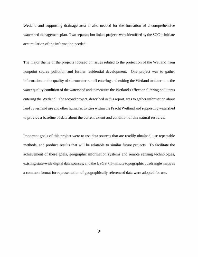
Wetland and supporting drainage area is also needed for the formation of a comprehensive

watershed management plan. Two separate but linked projects were identified by the SCC to initiate

accumulation of the information needed.

The major theme of the projects focused on issues related to the protection of the Wetland from

nonpoint source pollution and further residential development. One project was to gather

information on the quality of stormwater runoff entering and exiting the Wetland to determine the

water quality condition of the watershed and to measure the Wetland's effect on filtering pollutants

entering the Wetland. The second project, described in this report, was to gather information about

land cover/land use and other human activities within the Pracht Wetland and supporting watershed

to provide a baseline of data about the current extent and condition of this natural resource.

Important goals of this project were to use data sources that are readily obtained, use repeatable

methods, and produce results that will be relatable to similar future projects. To facilitate the

achievement of these goals, geographic information systems and remote sensing technologies,

existing state-wide digital data sources, and the USGS 7.5-minute topographic quadrangle maps as

a common format for representation of geographically referenced data were adopted for use.

4

Introduction

The purpose of the project was to conduct an inventory of land use and vegetation cover within the

watershed that drains into the Pracht Wetland. Products from this inventory are intended to assist

implementation of the Watershed Protection Approach demonstration project. Land use and

vegetation cover were identified and delineated on digital orthorectified aerial photography and

updated with current aerial slide photography. Field reconnaissance was conducted to assess the

accuracy and consistency of the interpretations. After detecting and resolving any procedural

problems, interpretations were edited and final geographic information systems (GIS) coverages and

grids were produced and delivered to the Kansas State Conservation Commission.

In addition to Land Cover, seven other GIS datasets and coverages were produced (or acquired) and

delivered. They were 1) the Watershed Boundary for the Pracht Wetland, 2) the 1982 Pracht

Wetland Boundary, 3) the Public Land Survey, 4) the Topographic Quadrangles; 5) the Digital

Elevation Models, 6) the 1991 Orthorectified Photography, and 7) the 1994 Rectified Photography.

Materials and Methods

The air photo interpretation and digitizing methodologies used in this project incorporate well-

established techniques and procedures. A brief description these methods is provided in this section.

An in-depth discussion of the air photo interpretation methods used in this project is found in

Campbell (1983). The digitizing methods used in this project are documented in Kansas Standards

and Procedures for Database Development (1991).

5

Data Sources

Information sources from which land use/land cover classes were interpreted and classified were

1991 National Aerial Photography Program (NAPP) black-and-white 9" x 9" transparencies and

1994 Agricultural Stabilization and Conservation Service (ASCS) natural color aerial slides acquired

during the most recently available summer flight periods (see Table 1). Two time periods in 1994

were acquired, early June and late July. The NAPP transparencies cover an area slightly larger than

5 miles by 5 miles and are centered approximately on one-quarter of a 7.5-minute topographic

quadrangle (often referred to as a quarter-quad). The ASCS photography covers an area slightly

larger than 1 mile by 2 miles. In addition to the NAPP transparencies, a Report of Calibration of

Aerial Mapping Camera was obtained from the U.S. Department of Agriculture, Aerial Photography

Field Office. This report contained camera parameters necessary for performing the

orthorectification of the NAPP imagery, a process which is described later.

USGS 7.5-minute topographic quadrangle maps were also acquired and were used for three tasks.

First, they were used to index slides to the proper township, range and section. Second, the

topographic maps were used to define the "Watershed Boundary" for the wetlands. The maps were

originally compiled in 1961 from aerial photography taken in 1954-1955 (Table 2). They were

photorevised in 1982. Third, the wetland area as depicted on the revised quadrangle was digitized

to use as a historical reference of its extent. 1:24,000 scale digital line graph (DLG) data of the

Public Land Survey System (PLSS) for these quadrangles were also acquired. The DLG data were

obtained from the State of Kansas Data Access and Support Center (DASC).

6

Table 1. Aerial photography used in study.

Photography Program Media Formatand Type

Scale(approximate)

Month Year

ASCS1 35mm slide,natural color

1:110,000 June 1994

ASCS 35mm slide,natural color

1:110,000 July 1994

NAPP2 9" x 9"transparency, b/w

1:40,000 September 1991

1 ASCS - Agricultural Stabilization and Conservation Service (now called the Consolidated Farm Services Agency)2 NAPP - National Aerial Photography Program

Table 2. Dates of compilation and source photography for the 7.5-minute topographicquadrangles used in study. The Kansas Geological Survey's row/columnidentification for the quadrangle is also given.

TopographicQuadrangle

Row/ColumnIdentification

Year ofCompilation

Year ofPhotography

Photorevised

Maize 0838 1961 1954-1955 1982

Wichita West 0738 1961 1954-1955 1982

7

The final data source acquired was 1:24,000 Digital Elevation Model (DEM) data, which were

necessary for the orthorectification process. DEM data are a matrix of values which represent the

elevations corresponding to a grid of evenly-spaced points. For 1:24,000 DEM data, this interval

is 30 meters. The area covered by one DEM corresponds to a 7.5 minute topographic quadrangle,

which is the source data for the DEM (Figure 1). Elevation is given in meters. The DEM data were

also obtained from the DASC.

Land Use/Land Cover Classes and Minimum Mapping Unit

The land use/land cover classification scheme used is a Level IV taken or modified from Anderson

et al. (1976). The 23 photo-interpreted land use/land cover classes are:

1110 - Medium/High Density Residential1120 - Low Density Residential1131 - Farmstead (occupied)1132 - Farmstead (abandoned)*1200 - Urban/Commercial1401 - Street or Highway1402 - Railway*1403 - Sewage Treatment Plant*1700 - Other Urban or Built-up Land2110 - Cropland2111 - Cropland (irrigated)2120 - Cropland (contour plowing)2130 - Cropland (terracing)*2140 - Cropland (grass waterway)*2300 - Confined Feeding Area3100 - Grassland/Rangeland4110 - Forest4120 - Hedgerow5000 - Water6200 - Nonforested Wetland (periodically inundated areas with hydrophytic cover)7100 - Bare Ground*8100 - Other (identification and delineation of additional categories if the above do not

accurately describe a land use or cover)*9999 - Background*

Figure 1. Example of Digital Elevation Model data for the Wichita West Quadrangle.

8

Wichita West QuadrangleShaded Relief Digital Elevation Model

Universal Transverse Mercator Projection - Zone 14Scale: Approximately 1:75,000

9

Appendix A contains detailed definitions for these classes. Note that the classes indicated by an

asterisk (*) do not occur in the land cover inventory conducted for the Pracht Wetland. The

inclusion of these classes is intended to illustrate how additional classes might be incorporated into

this classification scheme for areas that are more complex than the Pracht Wetland.

The minimum mapping unit is the size of the smallest area mapped for a land cover class. The

minimum mapping unit for all classes was 0.1 hectare (approximately 30 meters x 30 meters or 100

feet by 100 feet). The minimum width mapped was approximately 10 meters (32 feet).

Field Observations

Field observations of the Pracht Wetland and watershed were conducted during mid-August of 1995.

Accurate interpretations require use of field observations as confirmation of manuscript maps, and

as a means of resolving uncertainties in the interpretation process. For this project, field

observations served three purposes. First, they furnished the interpreters an opportunity to match

ground conditions with field patterns as they appeared on the transparencies and aerial slides.

Second, the field observations provided an indication of the consistency and accuracy of the

interpretations. Third, the trip helped to refine the delineation of the watershed boundary. It must

be noted that local alterations to the drainage in and around the watershed have occurred and that

this boundary must be considered an approximation of its position.

The field observations were particularly beneficial in correctly distinguishing between occupied and

abandoned farmsteads. An initial identification was made from the transparencies and slides. This

10

was done by looking for clues to human activity. These clues included presence of automobiles,

condition of driveways and parking areas (e.g., were they overgrown with vegetation?), and general

condition of the property (e.g., did lawns and buildings appear to be maintained?). Final

identification was made in the field. No door-to-door canvassing was conducted. However, careful

observations of a property easily revealed whether it was occupied or abandoned. Abandoned

farmsteads offered clues such as broken windows, sagging porches, holes in the roofs and overgrown

yards. Occupied farmsteads offered reverse clues- painted and well-maintained homes, manicured

yards and gardens, and other such signs of human habitation.

General Interpretation Strategy and Digital Tiling Scheme

A common interpretation strategy is to interpret and digitize discrete areal units based on some

regular and widely recognized map unit such as the 7.5-minute topographic quadrangle. These map

units are commonly referred to as a tiles. The delivered products are organized around the 7.5-

minute quadrangle tiling scheme. However, because the area for the Pracht Wetland and associated

watershed is slightly less than one-quarter of a quadrangle, but overlaps into two (2) quadrangles,

the interpretation strategy employed in this study combined the two quadrangle portions into one

continuous area.

This tactic had two practical benefits. First, the two digital NAPP photos were digitally spliced

together for later interpretation and map compilation. Second, it eliminated edge-matching

procedures (and their concurrent problems) that would have been necessary if the data had been

compiled individually from the two quadrangles.

11

Evaluation of the Aerial Photography

The NAPP transparencies were obtained from the U.S. Geological Survey-Earth Resources

Observation Systems (EROS) Data Center in Sioux Falls, SD. The ASCS aerial slides were

obtained from the Sedgwick County ASCS office. Both data sets were examined upon arrival to

assure that the order was correctly filled and to assess the quality of the transparencies and slides.

The slides were then keyed to the appropriate township-range-section on the topographic maps to

determine the proper slide orientation.

The spatial and spectral quality of the NAPP black-and-white transparencies was very good.

The spatial and spectral quality of the ASCS natural color slides was generally good. Some slides,

however, were difficult to interpret because of poor spatial resolution (due to poor camera focus)

and some were difficult to interpret because of poor color contrast. For example, the texture of the

vegetation shown in the slide is the basis for determining many land cover classes. In some of the

less clear slides, it was difficult to determine the crop management practice because the texture was

smeared. When colors were unclear, it was sometimes difficult to distinguish between agricultural

land and pastures. These problems were overcome by using all three photo sets, and by using the

surrounding area for clues to assist correct identification.

NAPP Orthorectification

An orthorectified digital NAPP photo was produced to provide an extremely accurate base map on

which interpretations could be delineated. Orthorectification is the process of creating a "geocoded"

image by using a DEM and a source image and its rational functions. Rational functions are two-

12

dimensional polynomials formed to handle the mapping of ground coordinates to image space,

where image space is the relationship of camera fiducial marks to documented camera parameters.

In this process, all effects of relief displacement and photographic perspective are eliminated and

each new output image pixel represents a precise horizontal position in the chosen coordinate system

(e.g., UTM).

The orthorectification process requires digital images as one of the inputs. To create the digital

images, the NAPP transparencies were scanned on a Hewlett-Packard ScanJet IIcx flat-bed scanner

at a resolution of 300 dots per inch (dpi). Given a photo scale of 1:40,000 and this scanning

resolution, the output image pixel resolution was approximately 3.4 meters.

In addition to the digital images, orthorectification requires ground control points and tie points.

Ground control points are known map x,y locations that can be readily identified on the digital

photo, usually a section corner. Tie points are locations that can be readily identified on two or more

digital photos.

The map ground control points were collected using a Calcomp 9100 series 36" x 48" digitizer

tablet. The resolution of the tablet is 50 lines/mm with an accuracy of ±0.127 mm and a

repeatability of 0.025 mm. Source material consisted of clean, tear-free and unfolded 7.5-minute

paper maps printed at 1:24,000 scale. The following brief description of ground control point

digitizing procedures adhere to Kansas Standards and Procedures for Database Development

(1991).

13

Quadrangle corners were used as tic registration points and were numbered clockwise from the

upper left. The geographic coordinates of the corners were projected to Universal Transverse

Mercator (UTM) Zone 14 coordinates and all subsequent entry of x,y coordinate data was recorded

in single precision meters. Accuracy of the map/digitizer setup was held to a root mean square error

(RMSE) of ±.003 inches or less. Positional accuracy of the setup was tested against 8 known map

coordinates located around the edge of the quadrangle. These points were within ±.005 inch of their

expected location (±3 meters or ±10 feet at scale). The map ground control points were then

digitized and recorded for input to the orthorectification program. The 1982 wetland boundary was

also digitized at this time from the Wichita West quadrangle.

The digital photo ground control points, tie points, and camera fiducial marks appearing on the photo

were collected by displaying the digital photo on a 20-inch monitor and interactively digitizing the

image x,y coordinates. These coordinates, the digitized map coordinates, and the camera parameters

were then loaded in to the software that performed the orthorectification.

The output orthorectified image was resampled to a spatial resolution of 2.0 meters. The input data

produced an RMSE for X of ±3.6 meters and an RMSE for Y of ±3.2 meters. The spatial accuracy

of the orthophoto was visually evaluated by digitally overlaying the 1:24,000 DLG PLSS on top of

the image (Figure 2). The PLSS section corners lie within 2 pixels of the photo intersection, and

often are at the photo intersection. This assessment means that the spatial accuracy of the

orthophoto is approximately ±4 meters (13.1 feet), which exceeds National Mapping Standards for

spatial accuracy.

Figure 2. Public Land Survey overlayed on the orthorectified 1991 NAPP photography.

14

Pracht Wetlands Watershed - September 1991Public Land Survey and Watershed Boundary

Universal Transverse Mercator Projection - Zone 14Scale: Approximately 1:45,000

15

ASCS Slide Rectification

The ASCS slides were rectified to match the UTM projection. Simple rectification is similar to

ortho-rectification, except that correction for terrain displacement is not performed. The

rectification of ASCS slide photography is also less precise because the slides do not have camera

fiducial marks necessary for precision rectification nor are there camera parameters that would allow

precision mapping of slide geometry to projection geometry. However, despite these limitations,

the rectification of slide photography produces products that have a spatial precision (or error) of

approximately ±8 meters (26 feet).

To rectify the slides, they were first scanned (digitized). The scanning was performed by a

commercial firm, which placed the digital slides onto a CD-ROM disk using the Kodak CD Photo

format. Software was used to convert from this original format to the ERDAS format used to do the

rectification. The digital slides had an original spatial resolution of approximately 1.3 meters.

Like orthorectification, simple rectification requires ground control points. The map ground control

points collected for the NAPP photo were used. The digital photo ground control points were

collected by displaying the photo on the monitor and interactively digitizing the image x,y

coordinates. The two sets of coordinates were then loaded in to the software that performed the

rectification.

Due to aircraft pitch, roll, and yaw, the ASCS slides are not geometrically correct. This means that

the transform equations used to convert the source image to a rectified image must correct for more

16

than linear distortions (i.e., 1st-order transforms can correct for changes in scale, skew, or rotation).

Higher order transforms are non-linear transformations and can correct nonlinear distortions such

as changes in camera perspective due to changes in aircraft orientation. A 2nd-order transform was

used to rectify all the slides.

The output rectified slides have a spatial resolution of 2.0 meters, like the NAPP digital photo. The

input data produced a range of RMSE from a low of ±5.8 meters to a high of ±9.9 meters. The

spatial accuracy of the rectified slides was visually evaluated by digitally overlaying the 1:24,000

DLG PLSS on top of the image (Figure 3). The PLSS section corners usually lie within the photo

road intersections, but occasionally fall just outside the road intersection.

It is important to note the differences between Figures 2 and 3, especially the growth in the

residential area just south of the Pracht Wetlands. This growth has occurred during the relative short

time span of 3 years. The field trip of 1995 revealed even more changes since the 1994 slide data.

These observations point out the necessity of using the most recent data available.

Photo Interpretation and Splitting the Coverages into Tiles

Interpretation of the photography was a two-step process. During the first step, "heads-up"

digitizing was used to create an initial land cover map. The orthorectified NAPP photo was

displayed on the monitor and the interpreter delineated areas of homogenous land cover by using

a mouse to draw

Figure 2. Public Land Survey overlayed on the orthorectified 1994 NAPP photography.

17

Pracht Wetlands Watershed - September 1994Public Land Survey and Watershed Boundary

Universal Transverse Mercator Projection - Zone 14Scale: Approximately 1:45,000

18

the boundaries. This technique resulted in the placement of land cover boundaries with a spatial

accuracy equivalent to the accuracy of the orthophoto (±4 meters). Initial labeling of the delineated

areas was also done during this step. Label points were located near the center of a land cover

polygon and encoded with the appropriate land cover code.

A photo interpreter's scale from the University of Michigan School of Natural Resources was used

to determine percentage of canopy cover (Carow, 1954). Percentages of canopy cover in some

wooded areas was difficult to determine, and it is estimated that the forest category may have a

range of error of ±5%. For example, wooded areas were classified as forest if they had a canopy

closure of 50% or greater. They may actually have only 45% canopy closure. Cases such as this

are believed to be few in number.

Tree hedgerows were also identified and delineated during this step. Hedgerows were defined as

being one tree wide, with the spacing between trees less than the diameter of their crowns. Because

this land cover feature is difficult to delineate because it is usually long and very narrow, it was

initially symbolized and digitized as a line. To convert this linear feature into an area, a GIS

buffering command was used with a buffer distance of 6 meters. A 6-meter buffer created a 12-

meter wide (approximately 40 feet) representation of the hedgerow. This figure was derived by

averaging several field measurements of hedgerows. The hedgerow coverage was then added to the

main land cover coverage.

19

The second step used the more recent ASCS aerial slides to update and finalize the initial

classification. Again, "heads-up" digitizing was used. The rectified ASCS photography was

displayed on the monitor and the interpreter identified changes between the 1991 NAPP data and

the 1994 ASCS data, delineating areas of changed land cover with the mouse. New or updated label

points were located near the center of a land cover polygon and encoded with the appropriate land

cover code. Note that nearly all of the change occurred along the urban fringe.

Because the ASCS slides are not as geometrically correct as the orthorectified NAPP photography,

some positional inaccuracies with the slides are to be expected. However, these errors were not

critical given that 1) the areas that were updated were few and small, and 2) the minimum map unit

size of approximately .10 hectares, or .25 acres, was small so that such errors represent only a small

percentage of the area for any map unit.

Topology was created for the coverage after digitizing the updated information. The topology

process (the building of explicit definition of relationships between graphic elements), identifies any

polygons that were not closed, polygons that had no label, polygons that had multiple labels, and

arcs that extended beyond their intended end-point, among several possible topological errors. All

errors encountered at this stage were corrected.

The cleaned coverage was then split into 7.5-minute topographic quadrangle tiles using the PLSS

coverage as a digital "cookie cutter". Figure 4 presents the cleaned, mapjoined coverage for land

cover in the Pracht Wetland.

20

Figure 4. Land Cover in the Pracht Wetland and Watershed.

21

A low-tech alternative for utilizing ASCS slide photography could have also been used to update

the 1991 data. For example, mylar overlays plotted with the DLG-PLSS and the initial

interpretations at a scale of 1:24,000 for a quadrangle would be produced. The mylar quadrangles

would then be placed on a drafting table fitted with a large piece of clear glass. The ASCS aerial

slides would then be back-projected onto the mylar overlay using a standard slide projector. Section

lines appearing on the slide, usually linear features such as roads, would then be matched to the

plotted section lines on the mylar. A matching procedure using a "best-fit" juggling of the projector

orientation and lens magnification could bring the slides into "rectification" with the plotted data.

While this procedure does not produce a photogrammetrically or planimetrically correct projection

of the slide, it should be possible to fit photo corner sections to within ±.01 of an inch (±20 feet at

scale) of the plotted section corners. These procedural techniques and the data transfer equipment

will introduce some positional error. For example, the lines drawn around any cover type will often

produce marks wider than the actual division. To minimize spatial errors, land cover should be

updated one section at a time. Changes noted between the 1991 NAPP data and the 1994 ASCS data

would be delineated as updates on the mylar with pencil and assigned a landcover class code

number. The updated mylar would then be digitized using procedures as outline earlier.

22

Project Results

All data entered into the database were printed, proofread, checked for proper topology, and

compared with the source data (quality control). The 1991 updated land cover coverage was

digitally overlayed on the orthophoto and linework compared with the image. In no instance was

a deviation of greater than one pixel (2 meters) observed.

For the land use/land cover data set, ground truth was collected for much of the Pracht Wetland and

associated watershed during the field trip in August of 1995. Although access to private land was

limited, a reasonably representative survey was conducted using public roads and elevated

observation points at a few publicly accessible sites to confirm the consistency and accuracy of the

interpretations. A systematic collection of ground level information was designed utilizing transects

along section lines. Of over 80 individual fields and parcels visited, only 8 were misidentified. This

gives an initial accuracy estimate of roughly 90 percent correct. These mislabelings were corrected.

Identification of these errors led to a better understanding of the reasons why they were

misidentified. For example, the majority of the errors were misidentifications of low density

residential areas as a farmsteads. The other errors that were encountered were a result of the

difference in time between the most recent aerial photo record (July 1994) and the field survey date

(August 1995). For example, three small fields lying on the urban fringe had been converted to

commercial use since July 1994. One forest polygon was found mistakenly labeled as cropland.

This error was traced to a blunder in data entry. Procedures designed to minimize mislabelings

23

would include the use of other reference photography and proof-reading of the draft map by a second

individual. The best professional estimate of accuracy for the map is 95 percent or greater (i.e., the

label correctly describes the delineated area).

Delivered Products

In addition to this report, one (1) quarter-inch cartridge tape containing two (2) Unix TAR format

files was delivered. Each tape TAR file contains coverages in the Arc/Info EXPORT format (*.e00

files) and corresponding documentation files (ASCII format). Note that the data obtained from

DASC (DEM and PLSS) do not have documentation files. Documentation for these data sets can

be obtained from the U.S. Geological Survey (1986 and 1987, respectively).

The first TAR file contains EXPORTed coverages and grids tiled according to the USGS 7.5-minute

quadrangles. The NAPP orthophoto and ASCS rectified photomosaic imagery are also on the first

tape file, in ERDAS image file format (*.lan files). The export files were named using the 8.3

naming convention. The root of a file name was formed using a 3- or 4-character mnemonic of the

coverage and using the 4-number KGS row/column identification system for 7.5-minute quadrangles

(see Table 2). Table 3 lists the coverage mnemonics used in the naming system. For example, the

file name for the Land Cover for Maize quadrangle is land0838.e00 and the file name for the 1982

Wetland for the Wichita West quadrangle is wet0738.e00. The documentation files for these files

are land0838.doc and wet0738.doc, respectively.

24

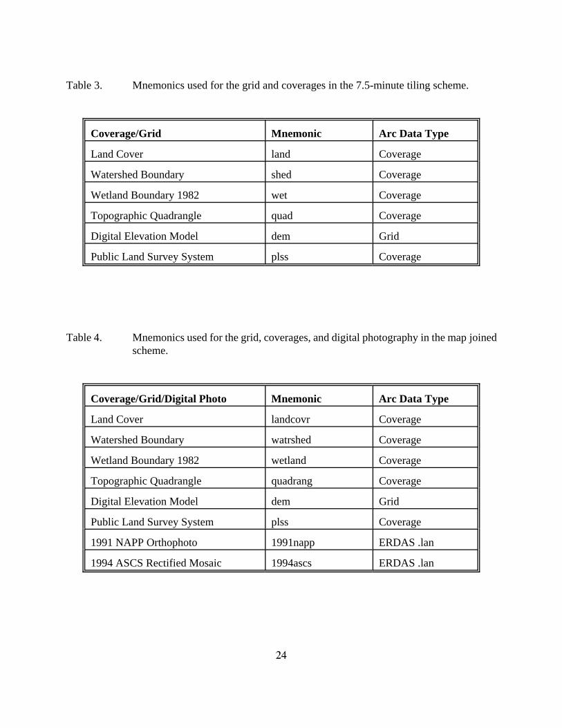
Table 3. Mnemonics used for the grid and coverages in the 7.5-minute tiling scheme.

Coverage/Grid Mnemonic Arc Data Type

Land Cover land Coverage

Watershed Boundary shed Coverage

Wetland Boundary 1982 wet Coverage

Topographic Quadrangle quad Coverage

Digital Elevation Model dem Grid

Public Land Survey System plss Coverage

Table 4. Mnemonics used for the grid, coverages, and digital photography in the map joinedscheme.

Coverage/Grid/Digital Photo Mnemonic Arc Data Type

Land Cover landcovr Coverage

Watershed Boundary watrshed Coverage

Wetland Boundary 1982 wetland Coverage

Topographic Quadrangle quadrang Coverage

Digital Elevation Model dem Grid

Public Land Survey System plss Coverage

1991 NAPP Orthophoto 1991napp ERDAS .lan

1994 ASCS Rectified Mosaic 1994ascs ERDAS .lan

25

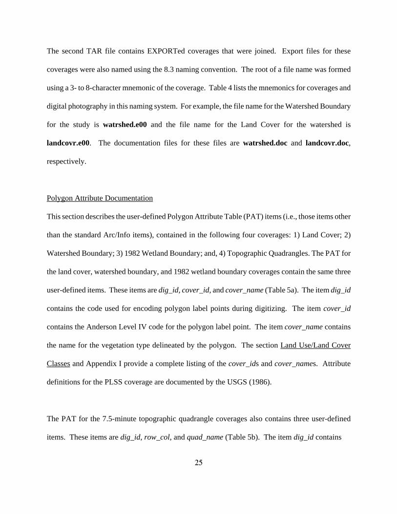
The second TAR file contains EXPORTed coverages that were joined. Export files for these

coverages were also named using the 8.3 naming convention. The root of a file name was formed

using a 3- to 8-character mnemonic of the coverage. Table 4 lists the mnemonics for coverages and

digital photography in this naming system. For example, the file name for the Watershed Boundary

for the study is watrshed.e00 and the file name for the Land Cover for the watershed is

landcovr.e00. The documentation files for these files are watrshed.doc and landcovr.doc,

respectively.

Polygon Attribute Documentation

This section describes the user-defined Polygon Attribute Table (PAT) items (i.e., those items other

than the standard Arc/Info items), contained in the following four coverages: 1) Land Cover; 2)

Watershed Boundary; 3) 1982 Wetland Boundary; and, 4) Topographic Quadrangles. The PAT for

the land cover, watershed boundary, and 1982 wetland boundary coverages contain the same three

user-defined items. These items are dig_id, cover_id, and cover_name (Table 5a). The item dig_id

contains the code used for encoding polygon label points during digitizing. The item cover_id

contains the Anderson Level IV code for the polygon label point. The item cover_name contains

the name for the vegetation type delineated by the polygon. The section Land Use/Land Cover

Classes and Appendix I provide a complete listing of the cover_ids and cover_names. Attribute

definitions for the PLSS coverage are documented by the USGS (1986).

The PAT for the 7.5-minute topographic quadrangle coverages also contains three user-defined

items. These items are dig_id, row_col, and quad_name (Table 5b). The item dig_id contains

26

Table 5a. Item definitions for the coverages Land Cover, Watershed Boundary, and 1982Wetland Boundary.

Item Name InternalWidth

Output Width Type Number of DecimalPlaces

AREA 4 12 F 3

PERIMETER 4 12 F 3

<cover_name># 4 5 B -

<cover_name>-ID 4 5 B -

DIG_ID 4 5 B -

COVER_ID 4 5 B -

COVER_NAME 52 53 C -

Table 5b. Item definitions for the coverage Topographic Quadrangles.

Item Name InternalWidth

Output Width Type Number of DecimalPlaces

AREA 4 12 F 3

PERIMETER 4 12 F 3

QUAD# 4 5 B -

QUAD-ID 4 5 B -

DIG_ID 4 5 B -

ROW_COL 4 5 B -

QUAD_NAME 16 17 C -

27

the code used for encoding polygon label points during digitizing. The item row_col contain the

quadrangle identification numbering system used by the Kansas Geological Survey (KGS) and the

Data Access and Support Center. The item quad_name contains the quadrangle name as it appears

on the USGS 7.5-minute quadrangle sheet.

Conclusions

This project demonstrates the application of digital NAPP orthophotography and digital ASCS slides

to mapping land use/land cover for wetland planning and management. The data sources used are

readily available (or soon will be) at little or no cost. The methods used and presented in this report

incorporate sound and well-established techniques and procedures. Future SCC wetland mapping

projects should use the results of this demonstration project as a base from which to start.

The accuracy of land use/land cover maps is a function of the interpreter's skill and the timeliness

of the aerial photography from which interpretations are made. And while the skills of an interpreter

can be honed and improved with training and practice, there is no substitute for the use of recent

photography. The experience gained during this project confirmed this observation. The 1991

NAPP digital orthophotography does provide a superior spatial basemap for delineating field

boundaries. However, it contains information that is often outdated, especially in urban or

urbanizing areas. The use of recent ASCS photography is an excellent solution to updating

information taken from the NAPP photography.

28

Other digital datasets were obtained from DASC that were of potential use in completing the picture

of human activities in the Pracht Wetland watershed, but did not directly contribute to compiling the

land use/land cover map. These were contaminated and environmental monitoring sites

(CONTAMINATION dataset), hazardous facilities in metropolitan areas (RTK-HAZ dataset), and

the groundwater, stream, and effluent water quality monitoring sites (WATER-QUALITY). These

datasets were visually overlayed on to the watershed boundary to determine if any sites were in or

near the watershed. None were in the watershed, but one hazardous facility does lie approximately

1 mile southwest and downstream of the wetland. It is recommended that these data sources be used

in similar future projects.

29

Bibliography

Anderson, J.R., E.E. Hardy, J.T. Roach, and E.E. Witmer, 1976. A Land Use Land CoverClassification System for Use with Remote Sensor Data, U.S. Geological SurveyProfessional Paper 964.

Campbell, J.B. 1983. Mapping the Land: Aerial Imagery for Land Use Information. Associationof American Geographers, 96 p.

Carow, J. 1954. The University of Michigan Photo-Interpreters Scale. School of Forestry,University of Michigan, Bulletin No. 6, 2 p.

Technical Advisory Committee of the Kansas GIS Policy Board, 1991. Kansas Standards andProcedures for Database Development. State of Kansas Geographic Information SystemsTechnology Management Program, 14 p.

United States Geological Survey, 1986. Digital Line Graphs from 1:24,000-Scale Maps: DataUsers Guide 1, National Mapping Program, Technical Instructions, United StatesDepartment of the Interior, Reston, VA, 109 p.

United States Geological Survey, 1987. Digital Elevation Models: Data Users Guide 5, NationalMapping Program, Technical Instructions, United States Department of the Interior, Reston,VA, 38 p.

30

Appendix A: Land Use/Land Cover Classes

This appendix describes the land use/land cover classes outlined earlier in this report. Theclassification scheme is derived from the Level IV scheme of Anderson et al. (1976), withmodifications (for example, low density residential and hedgerows) to fit the goals of this inventory.Note that not all categories occur in the land cover inventory for the Pracht Wetland.

Land Cover Codes and Definitions

1110- Medium/High-Density Residential: residential land consists of areas of medium density,with a more or less even distribution of vegetative cover and houses, to high density,represented by the multiple-unit structures of apartment complexes. Linear residentialdevelopments along transportation routes extending outward from urban areas are includedin this category. Rural subdivisions not directly connected to the core of an urbanized areaare also included. The main buildings, secondary structures, and immediate surroundinglandscape are all included - houses, apartment complexes, streets, garages, driveways,parking areas, lawns, etc.

1120- Low-Density Residential: low-density residential land consists of areas where houses aresituated on lots of more than one acre on the periphery of urban expansion. As with the"Medium/High Density Residential" class, the main buildings, secondary structures, andimmediate surrounding landscape are all included - houses, garages, driveways, parkingareas, lawns, streets, etc. Rural farmsteads are not included in this category.

1131- Farmstead (occupied): occupied farmsteads are developed land that includes clusters ofbuildings associated with farmsteads. These areas were separated from the "Low DensityResidential" category on a contextual basis; they typically have a single house in associationwith several out-buildings and are located some distance from cities and rural subdivisions.They are commonly surrounded by cropland and/or grassland. The main building, secondarybuildings and immediate surrounding landscape are all included - farmhouse, barns, sheds,silos, any other buildings, mowed yard area, windbreaks, etc.

1132- Farmstead (abandoned): the description for abandoned farmsteads is the same as that forthe occupied farmsteads except that the farmstead is not inhabited.

1200- Urban/Commercial: urban/commercial land consists of areas of intensive use with muchof the land covered by structures. These areas are used predominantly for the manufactureand sale of products and/or services. This category includes the central business districts ofcities, towns, and villages; suburban shopping centers and strip developments; educational,governmental, religious, health, correctional and institutional facilities; industrial andcommercial complexes; and communications, power, and transportation facilities. The mainbuildings, secondary structures, and areas supporting the basic use are all included - officebuildings, warehouses, driveways, parking lots, landscaped areas, streets, etc.

31

1401- Street or Highway: the street or highway class consists of roadways and roadway right-of-ways that are wider than the minimum mapping width of 10 meters (32 feet). In practice,this class consists of improved two-lane highways and four-lane urban roads. Smaller two-lane roads in urban areas are included in the appropriate urban class (e.g., residential class).

1402- Railway: railway includes the track, raised road bed, and larger rail facilities such asstations, parking lots, switching yards, etc. Overland track and spur connections are mappedif they are wider than the minimum mapping width of 10 meters (32 feet).

1403- Sewage Treatment Plant: sewage treatment plants are identified by their location in ornear a town, and by the settling ponds that typically feature regular shapes, such as squares,ovals, or rectangles.

1700- Other Urban or Built-up Land: other urban or built-up land consists of areas with usessuch as golf courses, zoos, urban parks, cemeteries, and undeveloped land within an urbansetting. This category also includes tracts of land that have been zoned residential orcommercial, but have yet to be developed.

2110- Cropland: cropland includes all areas in row crop and small grain, as well as harvestedland and large, uniform areas of bare ground on which there is no conservation managementpractice. The two dates of ASCS slides were particularly useful for cropland identificationwhen there was confusion as to whether a field was cropland or pasture. Cropped fieldscould often be differentiated using these data when they could not be clearly differentiatedusing black-and-white transparencies.

2111- Cropland (irrigated): the description for cropland (irrigated) is the same as that forcropland (class 2110), except that fields have some type of irrigation. The two predominanttypes are center-pivot and flood. Center-pivot irrigation is easily identified on aerial photosby their characteristic circle patterns. Flood irrigation is usually identified only by fieldobservation.

2120- Cropland (contour plowing): the description for cropland (contour plowing) is the sameas that for cropland (class 2110), except that furrows, produced by planting and tillageequipment running parallel to lines of equal elevation (contours) and perpendicular to theslope, are present. Contour plowing is a method to control soil erosion.

2130- Cropland (terracing): the description for cropland (terracing) is the same as that forcropland (class 2110), except that terraces (built-up ridges of soil), running parallel to linesof equal elevation and perpendicular to the slope, are present. Terracing is a method tocontrol soil erosion and conserve soil moisture by intercepting rain runoff.

2140- Cropland (grass waterway): the description for cropland (grass waterway) is the same asthat for cropland (class 2110), except that drainage paths within the field have been seededto either cool season or warm season grasses. These grassy drainage paths may be natural

32

or constructed. They are generally broad and shallow with a width in the 10's of feet, rarelyexceeding 100 feet.

2300- Confined Feeding Area: includes all confined livestock (i.e., cattle, horses, hogs, chickens,etc.) feeding and/or stabling operations. Feedlots are separated from other agricultural landbecause of their role as a potential pollution source. Feedlots are recognized by the largenumber of animals in a confined space, and the adjacent feed storage structures and sewagelagoons. In addition, larger feedlots can be found mapped as such on the USGS 1:24,000topographic maps used in the analysis, assuming that the feedlot is old enough to have beenmapped.

3100- Grassland/Rangeland: this category includes all pasture (hayland), rangeland, and othergrasslands having insufficient trees and/or shrubs to be classified as "Forest". Pastures andother grasslands are commonly found on lands that are rougher and more hilly thancroplands - therefore, in cases where it was difficult to distinguish a particular parcel, thetopographic map was used as an aid. Other resources were also used in distinguishingbetween cropland and pasture - see the discussion for the "Crop" category, above.

4110- Forest: wooded areas with greater than 50% canopy closure, based on comparison to thecrown closure scale on a University of Michigan School of Natural Resources photointerpreter's scale. Both deciduous and coniferous species are included in this category, withdeciduous trees being predominant.

4120- Hedgerow: unlike the "Forest" category, entries in the "Hedgerow" category are mappedas linear features. Typically occurring between agricultural fields, they are usually only onetree wide, making them very difficult to digitize with areal characteristics. To be delineatedas a hedgerow, the spacing of trees within the hedgerow does not exceed one-half the widthof a tree canopy. They are important features, commonly planted by earlier residents,lessening effects of wind and snow in some cases, and providing shade for livestock andhabitat for wildlife.

5000- Water: all water bodies not associated with sewage treatment or feedlots.

6200- Nonforested Wetland (periodically inundated areas with hydrophytic cover): nonforestedwetlands are those areas where the water table is at, near, or above the land surface for asignificant part of most years. They are frequently associated with topographic lows, suchas basins, playas, or potholes with no surface-water outflow. They are dominated byherbaceous vegetation or are nonvegetated (standing water or mud flat).

7100- Bare Ground: rock quarries, sand and gravel pits and other permanently exposed ground. Flooded pits are placed in the "Water" category.

33

8100- Other: the other category is reserved for land covers or land uses not defined previously. The use of the other category is discouraged in favor of defining a class within which thecover or use may be placed.

9999- Background : area outside of the interpreted watershed.

34

Addendum A: Summary Acreage for Land Covers in the Pracht Wetland (1994)

Cover Code Cover Name Acres

1110 Medium/High Density Residential 142.45

1120 Low Density Residential 40.83

1131 Farmstead (occupied) 27.12

1200 Urban/Commercial 2.08

1401 Street or Highway 16.89

1700 Other Urban or Built-up Land 7.75

2110 Cropland 896.26

2111 Cropland (irrigated) 468.59

2300 Confined Feeding Area 0.01

3100 Grassland/Rangeland 20.50

4110 Forest 11.12

4120 Hedgerow 2.43

5000 Water 10.84

6200 Nonforested Wetland 114.05

Total 1,760.92