practical applications in -...
TRANSCRIPT
Practical Applications in Digital Signal Processing

This page intentionally left blank
Practical Applications in Digital Signal Processing
Richard Newbold
Upper Saddle River, NJ • Boston • Indianapolis • San FranciscoNew York • Toronto • Montreal • London • Munich • Paris • Madrid
Capetown • Sydney • Tokyo • Singapore • Mexico City
Many of the designations used by manufacturers and sellers to distinguish their products are claimed as trademarks. Where those designations appear in this book, and the publisher was aware of a trademark claim, the designations have been printed with initial capital letters or in all capitals.
The author and publisher have taken care in the preparation of this book, but make no expressed or implied warranty of any kind and assume no responsibil-ity for errors or omissions. No liability is assumed for incidental or consequential damages in connection with or arising out of the use of the information or pro-grams contained herein.
The publisher offers excellent discounts on this book when ordered in quantity for bulk purchases or special sales, which may include electronic versions and/or custom covers and content particular to your business, training goals, marketing focus, and branding interests. For more information, please contact:
U.S. Corporate and Government Sales (800) 382- 3419 [email protected]
For sales outside the United States please contact:
International Sales [email protected]
Visit us on the Web: informit.com/ph
Library of Congress Cataloging-in-PublicationDataNewbold, Richard. Practical applications in digital signal processing / Richard Newbold. pages cm Includes bibliographical references and index. ISBN-13: 978-0-13-303838-5 (hardcover : alk. paper) ISBN-10: 0-13-303838-6 (hardcover : alk. paper) 1. Signal processing—Digital techniques. 2. Electric filters, Digital. I. Title. TK5102.9.N49 2013 621.382'2—dc23 2012024511
Copyright © 2013 Pearson Education, Inc.
All rights reserved. Printed in the United States of America. This publication is protected by copyright, and permission must be obtained from the publisher prior to any prohibited reproduction, storage in a retrieval system, or transmis-sion in any form or by any means, electronic, mechanical, photocopying, record-ing, or likewise. To obtain permission to use material from this work, please submit a written request to Pearson Education, Inc., Permissions Department, One Lake Street, Upper Saddle River, New Jersey 07458, or you may fax your request to (201) 236- 3290.
ISBN- 13: 978- 0- 13- 303838- 5ISBN- 10: 0- 13- 303838- 6
Text printed in the United States on recycled paper at Edwards Brothers Malloy in Ann Arbor, Michigan.First printing, October 2012
Executive EditorBernard GoodwinManaging EditorJohn FullerProject ManagerCaroline SenayProject EditorScribe Inc.Copy EditorScribe Inc.IndexerScribe Inc.ProofreaderScribe Inc.Publishing CoordinatorMichelle HousleyCover DesignerAnne JonesCover ArtLaura RobbinsCompositorScribe Inc.

To my wife, Mary, who has always stood by me through thick and thin.To my son Shannon, a brilliant software design engineer, and to my son Daniel, an accomplished attorney, both of whom were self- sufficient right out of college.

This page intentionally left blank
vii
ContentsPREFACE xiiiACKNOWLEDGMENTS xxiABOUT THE AUTHOR xxiii
1 REviEW OF DiGiTAL FREqUENCy 1
1.1 Definitions 2 1.2 Defining Digital Frequencies 2 1.3 Mathematical Representation of Digital Frequencies 9 1.4 Normalized Frequency 12 1.5 Representation of Digital Frequencies 13
2 REviEW OF COMPLEx vARiABLES 15
2.1 Cartesian Form of Complex Numbers 17 2.2 Polar Form of Complex Numbers 21 2.3 Roots of Complex Numbers 27 2.4 Absolute Value of Complex Numbers 35 2.5 Exponential Form of Complex Numbers 36 2.6 Graphs of the Complex Variable z 38 2.7 Limits 40 2.8 Analytic Functions 41 2.9 Singularity 42 2.10 Entire Functions 42 2.11 The Complex Number : 42 2.12 Complex Differentiation 43 2.13 Cauchy-Riemann Equations 47 2.14 Simply Connected Region 51
viii Contents
2.15 Contours 51 2.16 Line Integrals 52 2.17 Real Line Integrals 54 2.18 Complex Line Integrals 84 2.19 Cauchy’s Theorem 96 2.20 Table of Common Integrals 109 2.21 Cauchy’s Integral 109 2.22 Residue Theory 120 2.23 References 127
3 REviEW OF THE FOURiER TRANSFORM 129
3.1 A Brief Review of the Fourier Series 129 3.2 A Brief Review of the Fourier Transform 157 3.3 Review of the Discrete Fourier Transform (DFT) 187 3.4 DFT Processing Gain 254 3.5 Example DFT Signal Processing Application 261 3.6 Discrete Time Fourier Transform (DTFT) 263 3.7 Fast Fourier Transform (FFT) 267 3.8 References 268
4 REviEW OF THE Z-TRANSFORM 271
4.1 Complex Number Representation 271 4.2 Mechanics of the Z-Transform 274 4.3 Left-Sided Z-Transform 277 4.4 Right-Sided Z-Transform 278 4.5 Two-Sided Z-Transform 278 4.6 Convergence of the Z-Transform 279 4.7 System Stability 290 4.8 Properties of the Z-Transform 292 4.9 Common Z-Transform Pairs 304 4.10 Inverse Z-Transform 308 4.11 Pole and Zero Standard Form Plug-In Equations 334 4.12 Applications of the Z-Transform 350 4.13 Summary of Useful Equations 380 4.14 References 381
Contents ix
5 FiNiTE iMPULSE RESPONSE DiGiTAL FiLTERiNG 383
5.1 Review of Digital FIR Filters 384 5.2 Parks-McClellan Method of FIR Filter Design 392 5.3 PM Implementation of Half Band Filters 425 5.4 References 433
6 MULTiRATE FiNiTE iMPULSE RESPONSE FiLTER DESiGN 435
6.1 Poly Phase Filter (PPF) 436 6.2 Half Band Filter 465 6.3 Cascaded Integrator Comb (CIC) Filter 470 6.4 References 531
7 COMPLEx TO REAL CONvERSiON 533
7.1 A Typical Digital Signal Processing (DSP) System 534 7.2 Conversion of a Complex Signal to a Real Signal 540 7.3 Complex to Real Simulation Results 560 7.4 Reference 573
8 DiGiTAL FREqUENCy SyNTHESiS 575
8.1 Numerically Controlled Oscillator (NCO) 575 8.2 Enhanced NCO Phase Accumulator 608 8.3 NCO Synthesized Output Frequency Error 613 8.4 Adding a Programmable Phase Offset to the NCO Output 622 8.5 Design of an Industry-Grade NCO 628 8.6 NCO Phase Dither 641 8.7 References 644
9 SiGNAL TUNiNG 645
9.1 Continuous Time (Analog) Fourier Transform 647 9.2 Discrete Time (Digital) Fourier Transform 689 9.3 Useful Equations 754 9.4 References 759
x Contents
10 ELASTiC STORE MEMORy 761
10.1 Example Application of an Elastic Store Memory 762 10.2 PCM Multiplexing Hierarchy 763 10.3 DS-1C Multiplexer Design Overview 768 10.4 Design of the Elastic Store Memory 774 10.5 Hardware Implementation of the Elastic Store Memory 792 10.6 Overall DS-1C Multiplexer Design Block Diagram 801 10.7 Additional Information 803 10.8 References 805
11 DiGiTAL DATA LOCKED LOOPS 807
11.1 Digital Data Locked Design 808 11.2 Digital Data Locked Steady State Behavior 829 11.3 Digital Data Locked Transient Behavior 834 11.4 Data Locked Loop Bit-Level Simulation 845 11.5 Engineering Note 869 11.6 Summary of Useful Equations 869 11.7 References 871
12 CHANNELiZED FiLTER BANK 873
12.1 Introductory Description 873 12.2 Channelizer Functional Overview 877 12.3 Channelizer Detailed Design Concepts 919 12.4 Channelizer Software Simulation Results 962 12.5 Channelizer Hardware Design Example 967 12.6 Summary of Useful Equations 974 12.7 References 975
13 DiGiTAL AUTOMATiC GAiN CONTROL 977
13.1 Design of a Type I RMS AGC Circuit 981 13.2 Design of a Type II RMS AGC Circuit 1044 13.3 References 1047
Contents xi
A MixED LANGUAGE C/C++ FORTRAN PROGRAMMiNG 1049
A.1 Writing a C/C++ Main Program 1051 A.2 Calling Subroutines and Functions from a C/C++ Main 1051 A.3 Writing a FORTRAN Subroutine 1054 A.4 Writing a FORTRAN Function 1055 A.5 Passing Integer Arguments 1055 A.6 Passing Floating Point Arguments 1057 A.7 Passing Array Arguments 1059 A.8 Passing Pointer Arguments 1060 A.9 Compile/Link Mixed Language C/C++
FORTRAN Programs 1063 A.10 Parks-McClellan FORTRAN Subroutine Called from C Main 1064 A.11 References 1091
iNDEx 1093

This page intentionally left blank
xiii
Preface
I have spent more than 30 years toiling away as a digital hardware design engineer and as an unsophisticated self- taught software designer. Most of my software efforts were in support of my hardware designs and included en-deavors such as bit- level simulations, microcode generation, assembly code, FORTRAN, C/C++, and writing Microsoft Windows application graphics- oriented test stations, which I utilized to verify the proper operation of my digital creations.
I began my digital design career when digital signal processing (DSP) was still in its infancy. In those days, all digital designs were implemented with small-scale integrated (SSI) circuits that weren’t much more sophis-ticated than 4- bit adders and 8- to 1- bit multiplexers. The first company I worked for after graduation was heavily into the early phases of DSP.
DSP algorithms are for the most part dependent on repetitive multipli-cations and summation operations. The first digital multiplier I ever saw re-quired an entire chassis of equipment to do a 16- by- 16 multiplication. This multiplier consumed so much hardware that it was efficient to time- share it with other hardware that was engaged in processing independent tasks. De-vice propagation delays were so huge that building hardware systems that utilized a 5- MHz system clock was considered high tech.
To give some perspective about the state of the art at the time, the term Silicon Valley had not been coined yet. It was during this time that a little- known, small company that went by the name of Intel was operating out of a very tiny building located at 365 Middlefield Road in Mountain View, Cali-fornia. Intel had just introduced the world’s first microprocessor. It was a 4- bit machine called the 4004 microcomputer. It was built under contract to the Nippon Calculating Machine Corporation in Tokyo, Japan. With the introduc-tion of the 4004, the digital age changed gears. Digital technology soon began
xiv Preface
to evolve so quickly that hardware designed one year was almost obsolete by the next.
Program requirements always seemed to demand technology that wasn’t developed yet. Design engineers were constantly tasked with implementing tomorrow’s designs with today’s technology. This struggle, in a large sense, fueled an atmosphere of intense research and development and drove the in-dustry to continuously produce lower power, faster, and more complex de-vices and systems. Looking back, it seems like the world of DSP just exploded on all fronts. Start- up companies sprouted up in the Silicon Valley almost on a daily basis.
During this time, the science and technology of DSP grew and matured as integrated circuit manufacturers strived to produce higher speed signal processing components and lower power processors. Fusible link program-mable logic devices were introduced, which quickly evolved into repro-grammable logic devices and, over time, evolved into field programmable gate arrays (FPGAs), complex programmable logic devices (CPLDs), and application- specific integrated circuits (ASICs), which are still in use today. Other companies began to prosper by serving as fabrication houses for ex-tremely high- speed gallium arsenide and indium phosphide integrated cir-cuits. They would teach engineers how to design using their processes and then fabricate their application- specific designs.
The design tools necessary to support the programming and testing of these complex devices have evolved into big- time software applications. FPGA companies are even taking most of the challenges out of DSP design by offering a library of DSP circuits called cores that can be incorporated into an FPGA design with a simple keystroke, without much knowledge on the designer’s part of how these circuits operate.
During my 30- year career I have accumulated a fairly large library of DSP textbooks. With few exceptions, these books all cover the same basic topics. Different authors address the same subjects but each with their own unique approach. Reading several authors’ treatment of the same subject helped me view DSP processing techniques from different perspectives and tended to fill a lot of the blanks in my understanding of the subject. These books were well written by astute people in the field, and they all provided an excellent technical baseline for DSP design.
However, there have been few textbooks written that deal specifically with the many DSP topics and algorithms that are commonly used in every-day applied DSP. As a rule, a good working knowledge of these applied DSP algorithms usually comes from word of mouth, design mentoring, and de-sign experience. Over time, all design engineers accumulate (in their minds) a toolbox of circuits, procedures, algorithms, and techniques that are a product of years of long hours, a lot of sweat, tears, successes, failures, hand- wringing, and a fair amount of banging one’s head against the wall. Unfortunately these
Preface xv
toolboxes are not documented, and thus it is hard for other engineers to ac-cess the wealth of information contained within these toolboxes. Engineers for the most part are a secretive species and in their quest for job security are reluctant to publicize their hard- earned trade secrets.
There are many gray areas in DSP design that have not been addressed in detail by any of the engineering textbooks that I am familiar with. These gray areas usually don’t address questions like How do I design a circuit that will perform this or that critical DSP function?
For example, no DSP textbook I am familiar with has discussed in de-tail applications that are heavy into the use of complex digital signals, the spectra of real and complex digital signals, the science of complex to real sig-nal conversion, digital signal translation, or the concept of digital frequency synthesis.
I have not seen any text that provided a detailed analysis on how to design a numerically controlled oscillator (NCO) used in digital tuning ap-plications, or how to design an elastic store memory used in pulse code modulation (PCM) multiplexing applications, or how to design a digital data locked loop (DLL) or a digital automatic gain control (dAGC).
Other design topics rarely discussed in application- oriented detail by the myriad of DSP books available today include applications of poly phase filters (PPF) and cascaded integrator comb (CIC) filters, and applications like digital channelizers, sometimes referred to as transmultiplexers. This versatile circuit is found in many applications, such as frequency division multiplex (FDM) to time division multiplex (TDM) conversion, mixing consoles, wide-band scanners, and the processing of wideband intercepts in radio astronomy, to name just a few. All these subjects and more can be lumped into the gen-eral topic of Practical Applications in Digital Signal Processing.
THE PURPOSE OF THiS BOOK
The purpose of this book is to unlock and dispense some of the contents of my own personal toolbox in the hope of filling in some of these DSP gray areas. It is my hope to provide a source of usable information and DSP design techniques suitable for use in real- world design applications.
There are a great many DSP textbooks that are considered bibles of the DSP design world. Many of these books, along with technical papers writ-ten by astute people in the field, are referenced within this book. It is not the intention of this book to repeat the work that has been done by so many pre-vious authors. This book does not deal with the derivation and treatment of standard DSP concepts, which have been thoroughly addressed in great de-tail by many other authors. The sole purpose of this book is to serve as an
xvi Preface
application- oriented addendum to the many great DSP textbooks that have already been published.
WHO SHOULD READ THiS BOOK
This book is not intended for a person with no previous DSP knowledge or experience. This book is intended for the undergraduate and graduate stu-dent who will soon enter the signal processing industry. It is also intended for the engineer already in the industry who has some experience in DSP design and who is now searching for additional information regarding the design and implementation of common but largely undocumented DSP hardware or software applications.
HOW THiS BOOK iS ORGANiZED
This book is organized as a collection of tutorials on common DSP applica-tions. The first four chapters are detailed reviews on the mathematical tools necessary to successfully analyze, design, and build complex digital pro-cessing systems. The remaining nine chapters provide detailed tutorials on independent signal processing applications commonly used in the industry. An appendix is included that provides an in- depth discussion on mixed lan-guage programming. The content of each chapter is summarized in the fol-lowing sections.
Chapter 1: Review of Digital Frequency
This chapter is a short tutorial on digital frequency and how it is related to the system sample rate. It shows how to mathematically represent the value of a particular digital frequency and how to determine the value of all the samples in a digital sinusoidal waveform.
Chapter 2: Review of Complex variables
This chapter presents a thorough review of the subject of complex variables. After reading this chapter, it is possible for a person with no prior experience to become proficient in the use of this valuable mathematical tool in the de-sign and development of signal processing circuits and systems. The review starts by defining complex numbers and their properties and progresses all the way to a complete discussion of residue theory. The computation of resi-dues provides the engineer an easy alternative to compute the impulse re-sponse of a digital system.
Preface xvii
Chapter 3: Review of the Fourier Transform
This chapter provides an in- depth review of the Fourier series and both the continuous and discrete Fourier transform (CFT and DFT, respectively). The discussion includes the derivation of transform properties, transform pairs, Parseval’s theorem, and the derivation of energy and power spectral density (PSD) relationships. Attention is also given to the topic of spectral leakage, the band pass filter, and the low pass filter models of the DFT. Signal process-ing discussions include the use of windows, coherent and incoherent process-ing gain, and signal recognition. Even though this is an extensive review, it is written so that a reader without any background in the topics of Fourier se-ries or Fourier transforms can proficiently use them when working with sig-nal processing applications.
Chapter 4: Review of the Z- Transform
This chapter provides a comprehensive review of the z- transform. Detailed discussions include the use of pole-zero diagrams, inverse z- transforms, convergence, and system stability. A person with no prior knowledge of z- transforms can, after reading this chapter, utilize the knowledge gained to analyze complex digital systems, thereby enabling them to derive a system frequency response, determine system stability, and compute a system im-pulse response. In addition, the reader will learn how to use the z- transform in real- world situations to modify existing designs to either enhance perfor-mance or alter the specifications for incorporation into other systems.
Chapter 5: Finite impulse Response Digital Filtering
The focus of this chapter is on the design of finite impulse response (FIR) dig-ital filters. It is not my intent to repeat all of the excellent theoretical material that has already been published by so many astute authors. Almost all DSP texts devote substantial coverage to the history, theory, architecture, mathe-matics, and legacy design techniques of digital filters. Instead, the intent here is to concentrate solely on a single method for the design and implementa-tion of some of the more common filter types. The purpose of this chapter is twofold. First, in order to establish a communication baseline, we will pro-vide a very brief overview of digital filters. Second, we will demonstrate a computer- aided design methodology based on the Parks- McClellan optimal filter design program to implement several types of digital filters. A complete listing of this program is included in Appendix A.
Chapter 6: Multirate Finite impulse Response Filter Design
This chapter is a detailed discussion on the design of digital filters used to modify the sample rate of a signal. A designer is often faced with the task of
xviii Preface
either increasing or decreasing the sample rate of a signal by some integer or fractional amount. There are several methods that can be utilized to change the sample rate of a digital signal. All these methods involve the use of a digital filter, sometimes referred to as a multirate filter. Some multirate filters are better suited for specific rate change applications than others. In this chapter we will discuss three rate change methods that use the following three filter types:
1. Poly phase filters. The preferred method for moderate sized rate changes. 2. Half band filters. An efficient method for factor of two rate changes. 3. CIC filters. Computationally efficient filters for large rate changes.
Chapter 7: Complex to Real Conversion
This chapter provides a detailed tutorial on the conversion of a complex sig-nal to a real signal. This is a common signal processing function, yet material dealing with this very important topic is rarely found in engineering text-books. A very good example of complex signal processing is seen in digital systems that employ a front- end tuner. These systems fall into a category that can be loosely categorized as “digital radio,” in that an input wideband sig-nal is tuned up or down in frequency and passed through a band pass or low pass filter to isolate some narrow band of interest. The mathematics of the tuning function converts the real input signal into a complex signal. The fil-tered narrow band signal is then processed in its complex form to implement whatever the particular application requires. After the intermediate process-ing is complete, the complex signal is generally converted back to real and provided as an output.
Chapter 8: Digital Frequency Synthesis
There are numerous applications in the world of DSP that utilize a numeri-cally controlled oscillator, or NCO. An NCO is a programmable oscillator that outputs a digital sinusoid at some user- specified frequency and phase. The sinusoid can be fixed at some programmed frequency, or it can be swept or hopped over a band of frequencies. The sinusoid can have a constant phase or it can be programmed to have multiple or switched phases. It can be a sim-ple or a complex device, depending on the requirements of the application in which the NCO is used. A typical application utilizes the NCO to produce a programmable complex sinusoid to tune band pass signals down to base band for filtering and postprocessing, similar to the local oscillator in an AM radio. This chapter contains detailed figures that clearly illustrate both the de-sign of the NCO and the workings of all the internal processing functions. Ex-tensive simulations graphically illustrate the signals produced by the NCO.
Preface xix
Chapter 9: Signal Tuning
This chapter provides a thorough discussion on the subject of signal tuning in both the continuous analog and discrete digital domains. It is often necessary when processing a signal to move it from one region of the frequency spec-trum to another region. This is especially true when processing communica-tions signals, where a band limited signal centered at frequency f1 is tuned to another center frequency f2 in order to simplify downstream processing. This chapter illustrates the methods used to translate the spectrum of real and complex signals both up and down in frequency.
Chapter 10: Elastic Store Memory
During their careers, most engineers have designed interfaces between two or more data processing systems that utilized synchronous data streams. There are occasions, however, when a designer must interface two or more processing systems or data streams where the data rates are asynchronous to one another. For purposes of this chapter, the term asynchronous refers to the case where each data stream is time aligned to its own clock gener-ated by an independent clock oscillator. The frequency and phase of each clocked data stream are similar but not necessarily identical. Each clock os-cillator’s output frequency uniquely varies over time and temperature. In many cases, these clocks may differ by as much as a few thousand hertz. In this chapter we illustrate how to synchronize these systems with an elastic store memory.
Chapter 11: Digital Data Locked Loops
Suppose you are presented with a time division multiplex, or TDM, bit stream composed of a multiplex of two or more independent and originally asynchronous tributaries. How can we demultiplex these tributaries and syn-thesize an independent bit clock for each that is on average identical to its original premultiplex clock? This type of signal is similar to a high- level tele-phone PCM multiplex that carries several lower level tributaries. This is only one of many possible examples. The same question can be asked of any de-multiplex processing where the multiplexed tributaries were originally asyn-chronous to one another. The answer requires utilizing a digital data locked loop, or DLL. The DLL is a fairly simple device that uses an elastic store mem-ory to synthesize a bit stream clock and then synchronizes the demultiplexed bit stream or tributary with that clock, all with no prior knowledge of the original clock frequency. This chapter provides a thorough tutorial on how to design DLLs for just about any relevant application.
xx Preface
Chapter 12: Channelized Filter Bank
This chapter presents a high- level functional discussion followed by an in- depth, detailed tutorial on the design of a digital channelizer, sometimes re-ferred to as a transmultiplexer. As mentioned previously, this versatile circuit is found in many signal processing applications. The channelizer can easily replace hundreds of receivers with not much more than a single integrated circuit. In this chapter, we will design a working channelizer that simultane-ously processes up to 2000 independent equal bandwidth signals.
Chapter 13: Digital Automatic Gain Control
This chapter is a thorough discussion of a Type I and Type II digital auto-matic gain control, or dAGC. This subject matter is rarely covered in any en-gineering textbook available today, and if it is covered, it is usually given a cursory look amounting to not much more than a paragraph or two. In many electronic systems, one of the most important functions is automatic gain control (AGC). In general, an AGC is a nonlinear feedback circuit that if not designed properly can become unstable. The purpose of this chapter is to de-sign a dAGC circuit; derive its operational parameters; simulate it; and then graphically illustrate the transient response, the steady state operation of the loop error, the loop gain, and the circuit output in response to various input signals and input signal perturbations.
Appendix A: Mixed Language C/C++ FORTRAN Programming
Over the years, there is a good chance that engineers who have been in the business for a while have accumulated a few dusty, old FORTRAN programs, functions, or subroutines that represent some pretty valuable legacy code. If these coded routines weren’t considered to be so valuable, the engineers more than likely would never have saved them. Typically, these routines represent a treasure chest of tested, debugged, and proven code that is still relevant in today’s engineering environment. The one big problem is that most of the software today is developed in C or C++. If this is the predicament that you find yourself in, there is some good news and some bad news for you. The good news is there is a good chance that the program manager and design engineering staff has at their disposal a wealth of proven FORTRAN code. In-corporating this proven code into a project very well could result in a signifi-cant reduction in labor costs and a significant reduction in program schedule. The bad news, of course, is that C or C++ are today’s preferred languages; therefore writing deliverable code in FORTRAN is really not a viable option. So if you are a program manager or a design engineer, what can you do in a situation such as this? One alternative is to build a mixed language program, where the bulk of the code including the main is written in C/C++ and linked with one or more valuable FORTRAN legacy functions and/or subroutines. This appendix is a tutorial on how to do just that.
xxi
Acknowledgments
I extend my sincere appreciation to Bernard Goodwin, executive editor of Pearson North America, Prentice Hall Professional technical publications, for his generous help and support during the difficult task of introducing a new author to the world of technical publishing. I would also like to acknowledge Dr. John Treichler of Applied Signal Technology for his gracious permission to reference his original work on transmultiplexers.
I would like to thank Richard Lyons, author of Understanding Digital Sig-nal Processing (Prentice Hall); David Myers; Jim Kemerling; Michael Myers; and C. Britton Rorabaugh, author of Notes on Digital Signal Processing (Pren-tice Hall), for their technical review of the manuscript.
I would like to give a long overdue thank you to Mike Tate of Electromag-netic Systems Laboratories, the absolute best technician I have ever worked with, who helped me successfully begin my career so many years ago. I would like to thank Tom Ranweiler of Northrop Grumman, the most technically astute software design engineer I have ever worked with, who was the person who helped me finish my career on a successful note with the design of a unique special-purpose signal processing system. I am also thankful for the opportu-nity to have worked alongside the brilliant systems engineer Dr. Pin- Wei Chen of Northrop Grumman who helped keep me involved in internal research and development design projects.
Finally I would like to extend my deep appreciation to my wife Mary for her patience, support, understanding, and encouragement throughout this very long project.

This page intentionally left blank
xxiii
Richard Newbold received his B.S.E.E. and M.S.E.E. degrees in 1974 and 1978, respectively, and has spent more than 30 years as a digital hardware design engineer and self- taught software designer. His design experience in-cludes special-purpose signal processing hardware and computers that pro-cessed real time wideband signals, direct sequence spread spectrum system processors, PCM multirate processing systems, high- speed signal processing systems implemented on special-purpose gallium arsenide ASICs, transmul-tiplexers, channelizers, multirate filters, tuners, frequency synthesizers, DLLs, synchronous digital hierarchy (SDH) demultiplexers, fractional resamplers, adaptive filters, elastic store memories, adaptive beam forming, asynchro-nous clock recovery, and fault tolerant signal processors. His software expe-rience includes real time signal processing, bit- level hardware simulations, microcode and bit slice programming, assembly programming, FORTRAN, C/C++, and Microsoft Windows graphics- oriented test stations, which were used to bit- level simulate, graphically display, and verify the proper opera-tion of his digital creations.
About the Author

This page intentionally left blank
1
It is easy to mathematically represent an analog frequency on paper. The range of frequencies in the analog domain is both continuous and theoreti-cally infinite. If we use the symbol fO to represent some arbitrary analog fre-quency all we need to do is to equate it with any one of an infinite number of available frequencies. We could, for example, choose fO to be equal to 23.456 Hz, or we could just as easily choose fO to be equal to 1.005 MHz. We could choose just about any other value to any precision that we can dream up. As long as we remain realistic, there is no limit on the values that fO can take on.
However, a digital system operates on digital data and generates digital results that are valid only at discrete increments of time equal to the period of the system sample clock. Therefore the value that a digitally generated dis-crete frequency can take on is a small subset of the range of values available to analog frequencies. The discrete frequency values within this subset are di-rectly related to and dependent on the sample rate of the digital system clock.
This leads to some confusion when people deal with digital frequencies for the first time. Much of the confusion can be summed up with three fre-quently asked questions:
1. How do I define a digital frequency? 2. How do I mathematically represent a digital frequency? 3. How do I synthesize a digital frequency in hardware or software?
The scope of this chapter is to provide an answer for the first two of these questions. The answer to question number 3 requires its own chapter and is dealt with in detail in Chapter 8, “Digital Frequency Synthesis.”
Review of Digital Frequency
Chapter One
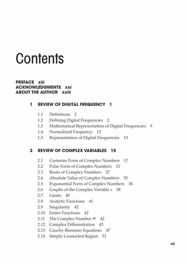
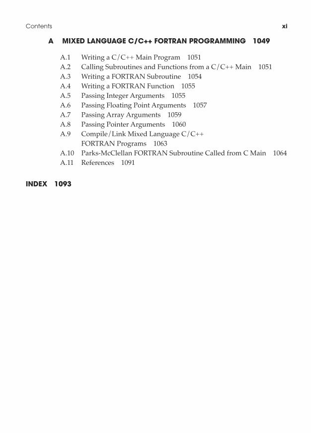
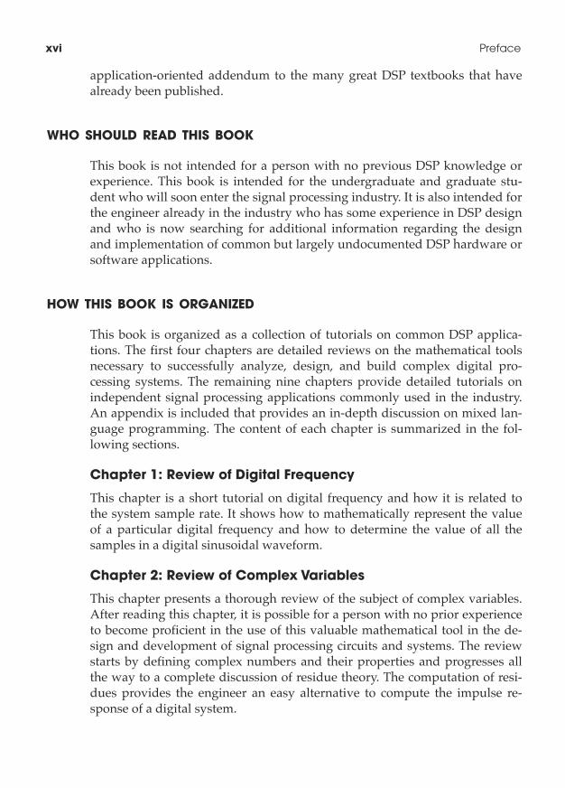
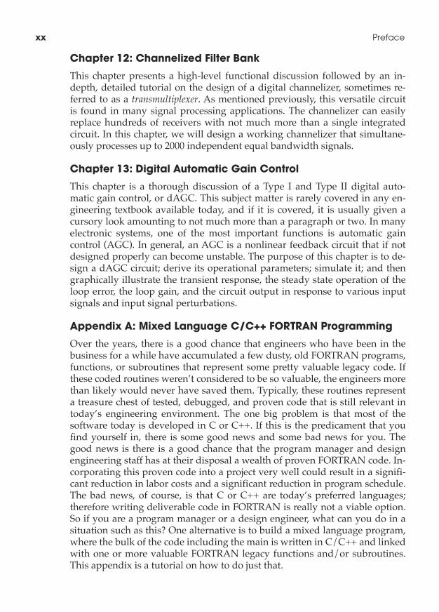
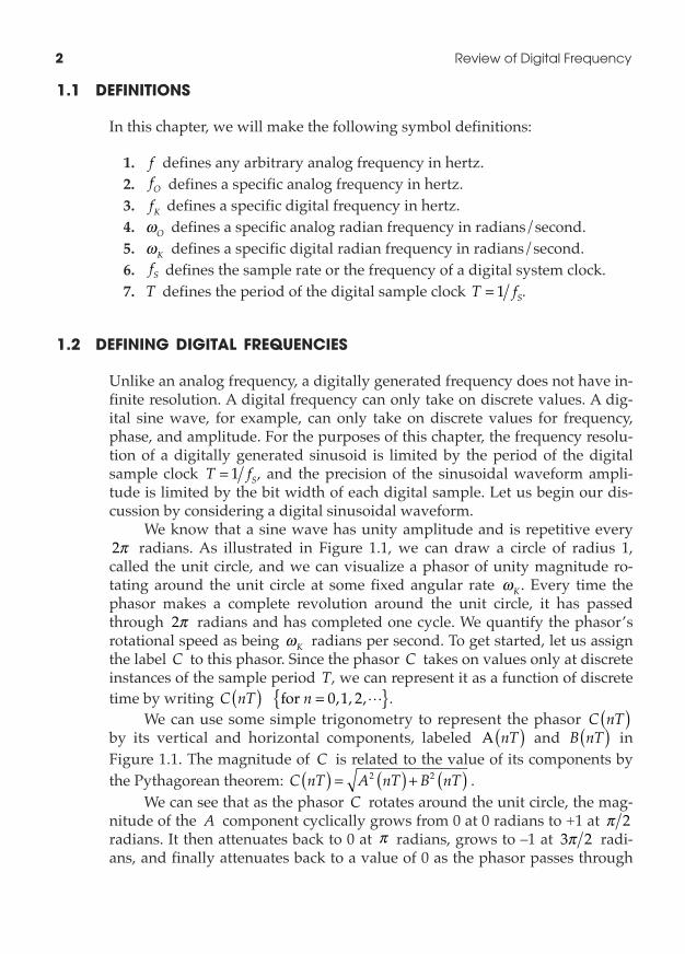
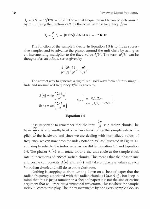
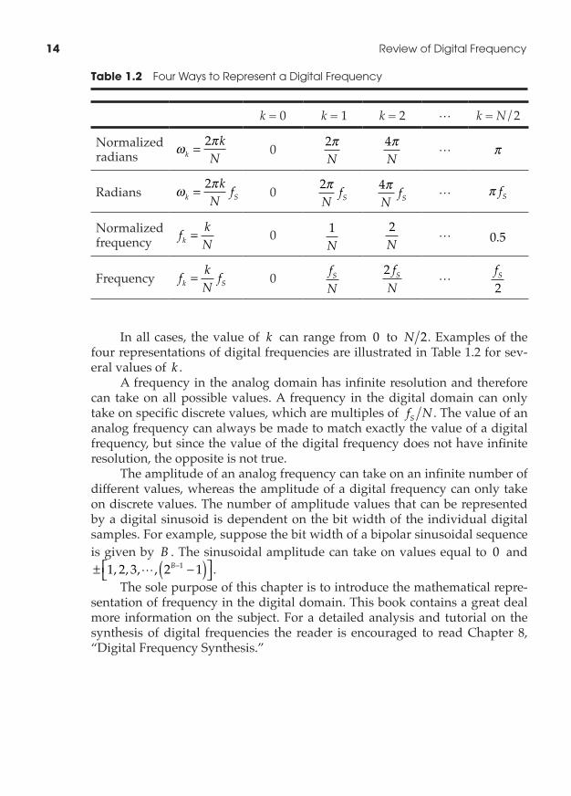
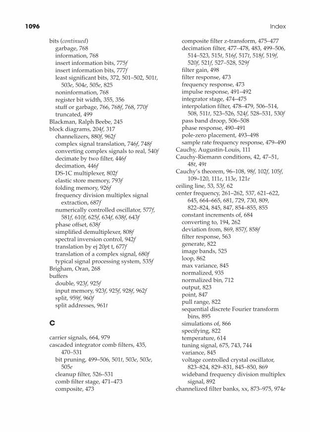
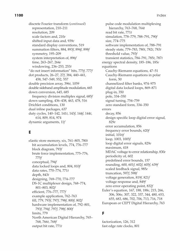
0 1 2 3 4 65 7 8 9 10 11 1312 14 15 k
Folding Frequency2, 2Sk N f f
16N
The frequencies above 2are folded or aliased down infrequency symmetric with thefolding frequency 2.
k N
k N
16
2� Review�of�Digital�Frequency
1.1 DefinitiOns
In this chapter, we will make the following symbol definitions:
1. f defines any arbitrary analog frequency in hertz. 2. fO defines a specific analog frequency in hertz. 3. fK defines a specific digital frequency in hertz. 4. ωO defines a specific analog radian frequency in radians/second. 5. ωK defines a specific digital radian frequency in radians/second. 6. fS defines the sample rate or the frequency of a digital system clock. 7. T defines the period of the digital sample clock T fS= 1 .
1.2 Defining Digital frequenCies
Unlike an analog frequency, a digitally generated frequency does not have in-finite resolution. A digital frequency can only take on discrete values. A dig-ital sine wave, for example, can only take on discrete values for frequency, phase, and amplitude. For the purposes of this chapter, the frequency resolu-tion of a digitally generated sinusoid is limited by the period of the digital sample clock T fS= 1 , and the precision of the sinusoidal waveform ampli-tude is limited by the bit width of each digital sample. Let us begin our dis-cussion by considering a digital sinusoidal waveform.
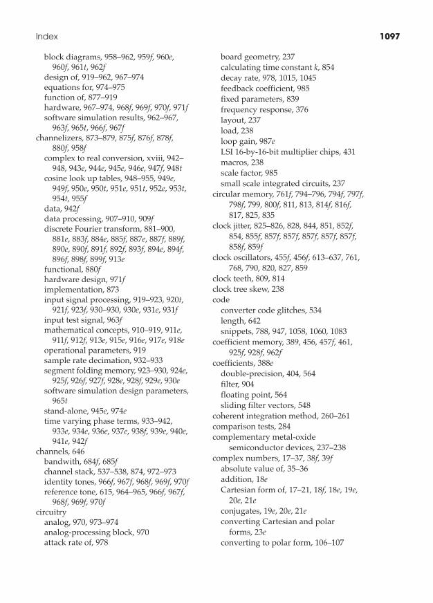
We know that a sine wave has unity amplitude and is repetitive every 2π radians. As illustrated in Figure 1.1, we can draw a circle of radius 1, called the unit circle, and we can visualize a phasor of unity magnitude ro-tating around the unit circle at some fixed angular rate ωK . Every time the phasor makes a complete revolution around the unit circle, it has passed through 2π radians and has completed one cycle. We quantify the phasor’s rotational speed as being ωK radians per second. To get started, let us assign the label C to this phasor. Since the phasor C takes on values only at discrete instances of the sample period T, we can represent it as a function of discrete time by writing C nT n( ) ={ } for 0 1 2, , , .
We can use some simple trigonometry to represent the phasor C nT( ) by its vertical and horizontal components, labeled A nT( ) and B nT( ) in Figure 1.1. The magnitude of C is related to the value of its components by the Pythagorean theorem: C nT A nT B nT( ) = ( ) + ( )2 2 .
We can see that as the phasor C rotates around the unit circle, the mag-nitude of the A component cyclically grows from 0 at 0 radians to +1 at π 2 radians. It then attenuates back to 0 at π radians, grows to –1 at 3 2π radi-ans, and finally attenuates back to a value of 0 as the phasor passes through
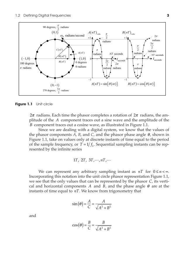
1.2� Defining�Digital�Frequencies� 3
2π radians. Each time the phasor completes a rotation of 2π radians, the am-plitude of the A component traces out a sine wave and the amplitude of the B component traces out a cosine wave, as illustrated in Figure 1.1.
Since we are dealing with a digital system, we know that the values of the phasor components A, B, and C, and the phasor phase angle θ , shown in Figure 1.1, take on values only at discrete instants of time equal to the period of the sample frequency, or T fS= 1 . Sequential sampling instants can be rep-resented by the infinite series
1 2 3T T T nT, , , , ,
We can represent any arbitrary sampling instant as nT for 0 ≤ < ∞n . Incorporating this notation into the unit circle phasor representation Figure 1.1, we see that the only values that can be represented by the phasor C, its verti-cal and horizontal components A and B, and the phase angle θ are at the instants of time equal to nT . We know from trigonometry that
sin θ( ) = =+
AC
AA B2 2
and
cos θ( ) = =+
BC
BA B2 2
figure 1.1 Unit�circle
0 degrees 0 radians
90 degrees, radians2
180 degrees radians
3270 degrees, radians2
radians/secondK
nT 1,0
0,1
1,0
0, 1
A nT
B nT
C nT
voltsA nT
0
2radians
radians
32
radians
1
1
2radians
secondsNT
secondst
2radians
radians
32
radians
1
1
2radians
secondsNT
voltsB nT
sinA nT nt cosB nT nt
secondst 0
4� Review�of�Digital�Frequency
We also know that since we are working on the unit circle, the magni-tude of C A B= + =2 2 1. Therefore we can state that at any sampling instant nT,
A nT nT( ) = ( ) sin θ
and
B nT nT( ) = ( ) cos θ
Equation1.1
So far so good, but how do we quantify the discrete values taken on by the sinusoidal waveforms? Well, we can start by dividing the unit circle into N equal arc segments, illustrated by the black dots on the unit circle in Figure 1.1. Each arch segment is a portion of the unit circle scribed by the tip of the phasor C as the phase angle θ is incremented by 2π N radians.
We will take this opportunity to coin a new and highly technical term. Let us define the angle 2π N and the arch segment it describes as a radian chunk. The angle between the adjacent black dots on the unit circle in Figure 1.1 is equal to a radian chunk. The phasor C nT( ) and its components A nT( ) and B nT( ) can only be evaluated at each black dot corresponding to each radian chunk on the unit circle. Therefore the maximum number of samples that can represent a single cycle of a digital sine wave is equal to N.
If the digital oscillator that is generating the digital sinusoid is operating with a sample clock of fS Hz , then the phasor C nT( ) would rotate around the unit circle in discrete radian chunks of 2π N at the clock rate of fS Hz.The lowest radian frequency of the digital oscillator can be mathematically defined as
ω πK SN
f=
2 radians sample
samplesecond = radians/second2π
NfS
ω πK SN
f= 2 radians/second
Equation1.2
The lowest or fundamental frequency of the digital oscillator can be mathematically defined as
1.2� Defining�Digital�Frequencies� 5
fN
fK S=
12
2π
π radians
radians sample
ssamplesecond
= second = Hz
−1 11
Nf
NfS S
fNfK S= 1 Hz
Equation1.3
If we think about it for a minute, Equation 1.2 and Equation 1.3 make sense. If the phasor points to each black dot on the unit circle for one sam-ple period, it will take N sample periods for it to move from dot zero to dot N − 1. In doing so, it will make one revolution of the unit circle stopping once at each black dot in N sample periods. It will take N sample periods to trace out exactly one sinusoidal cycle. The total period for each cycle will be equal to NT sec. The frequency of this sinusoidal cycle is then given by f NT f NS= ( ) = ( )1 second Hz. Therefore the frequency of the sinusoids
traced by the A nT( ) and B nT( ) components will be equal to f NS( )Hz.Let us look at a very simple example. Suppose we have a digital oscilla-
tor clocked with a sample clock of fS = 32 Hz, and suppose we decided that N will be 16. The unit circle is subdivided into 16 equal arc lengths, giving us 16 equal radian chunks. The rotating phasor C nT( ) will be evaluated at 16 locations around the unit circle. This means there will be 16 samples per each period of the synthesized sinusoidal waveform. The digital radian frequency would be
ω π πK =
216
radians 32 = 4 radianssec
//second
or, since fK K= ω π2 , we can easily compute the digital oscillator frequency to be
fK K= =
ωπ
ππ2
42
radians second radians
= 2 seecond Hz− =1 2
In this simple example, 2 Hz is the lowest frequency other than zero that our simple digital oscillator can generate. This is based on the value of the sample frequency fS and our choice for the value of N . If, for the same sample rate, we had chosen N to be a larger number, then the resolution of fK would have been greater. For example, if we had selected N = 64 , the
lowest frequency other than 0 Hz that our oscillator could produce would be
6� Review�of�Digital�Frequency
fNfK S= = =1 1
6432 0 5 Hz Hz Hz.
This is a good start, but a digital oscillator that can produce only a single frequency isn’t as useful as an oscillator that can be programmed to produce any one of a whole range of discrete frequencies. Ideally, we would like to be able to program the digital oscillator to output any one of a wide range of discrete frequencies. We can achieve this enhancement with the addition of a multiplier “k” in Equation 1.2 and Equation 1.3. We can rewrite these equa-tions to include the multiplier k such that
ω πK S
K S
kN
f
f kNf
k=
==
2
0 1 2radians second
Hzwhere , , , .... /N 2{ }
Equation1.4
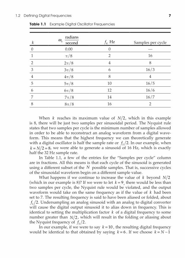
If k = 1 , then the frequencies represented by Equation 1.4 are identical to those represented by Equation 1.2 and Equation 1.3. The value of k can take on discrete integer values ranging from 0 to N 2 . In our previous example, we set fS = 32 Hz, and N = 16 so k could take on values of 0 1 2 3 4 5 6 7 8, , , , , , , , .All the possible frequency values that this example oscillator can take on are tabulated in Table 1.1.
As we can see from the table, this oscillator can be programmed to pro-duce one of nine possible frequencies with a resolution of 2 Hz. The addition of the variable k in Equation 1.4 causes the phasor C nT( ) to rotate around the unit circle in multiples of 2π N radian chunks at a rate of fS sample per second. When k is set to unity, the phasor will take on values at every black dot on the unit circle producing the oscillator’s lowest or fundamental fre-quency. In this case, each cycle of the generated sinusoid will be composed of N samples.
When k is set to 2, the phase angle of the phasor θ nT( ) will increase in increments of two radian chunks each tick of the sample clock. The phasor C nT( ) will take on the values of every second dot, and it will rotate around the unit circle twice as fast, producing a sine or cosine wave that is twice the fundamental frequency. In this case, each cycle of the sinusoid will be com-posed of half or N 2 samples. Similarly, when k is set to 4 the phasor will travel around the unit circle at four times the fundamental rate, taking on val-ues at every fourth dot to produce an output frequency that is four times the fundamental frequency. Each cycle, however, will be composed of N 4 num-ber of samples per cycle.
1.2� Defining�Digital�Frequencies� 7
When k reaches its maximum value of N 2, which in this example is 8, there will be just two samples per sinusoidal period. The Nyquist rule states that two samples per cycle is the minimum number of samples allowed in order to be able to reconstruct an analog waveform from a digital wave-form. This means that the highest frequency we can theoretically generate with a digital oscillator is half the sample rate or fS 2. In our example, when k N= =2 8, we were able to generate a sinusoid of 16 Hz, which is exactly half the 32 Hz sample rate.
In Table 1.1, a few of the entries for the “Samples per cycle” column are in fractions. All this means is that each cycle of the sinusoid is generated using a different subset of the N possible samples. That is, successive cycles of the sinusoidal waveform begin on a different sample value.
What happens if we continue to increase the value of k beyond N 2 (which in our example is 8)? If we were to let k = 9 , there would be less than two samples per cycle, the Nyquist rule would be violated, and the output waveform would take on the same frequency as if the value of k had been set to 7. The resulting frequency is said to have been aliased or folded, about fS 2. Undersampling an analog sinusoid with an analog to digital converter
will cause the digital output sinusoid it to alias down in frequency. This is identical to setting the multiplication factor k of a digital frequency to some number greater than N 2 , which will result in the folding or aliasing about the Nyquist frequency of fS 2.
In our example, if we were to say k = 10 , the resulting digital frequency would be identical to that obtained by saying k = 6 . If we choose k N= − 1
table 1.1 Example�Digital�Oscillator�Frequencies
k ωk radianssecond fK Hz Samples per cycle
0 0.00 0 —1 π/8 2 16
2 2π/8 4 83 3π/8 6 16/34 4π/8 8 45 5π/8 10 16/56 6π/8 12 16/67 7π/8 14 16/78 8π/8 16 2
8� Review�of�Digital�Frequency
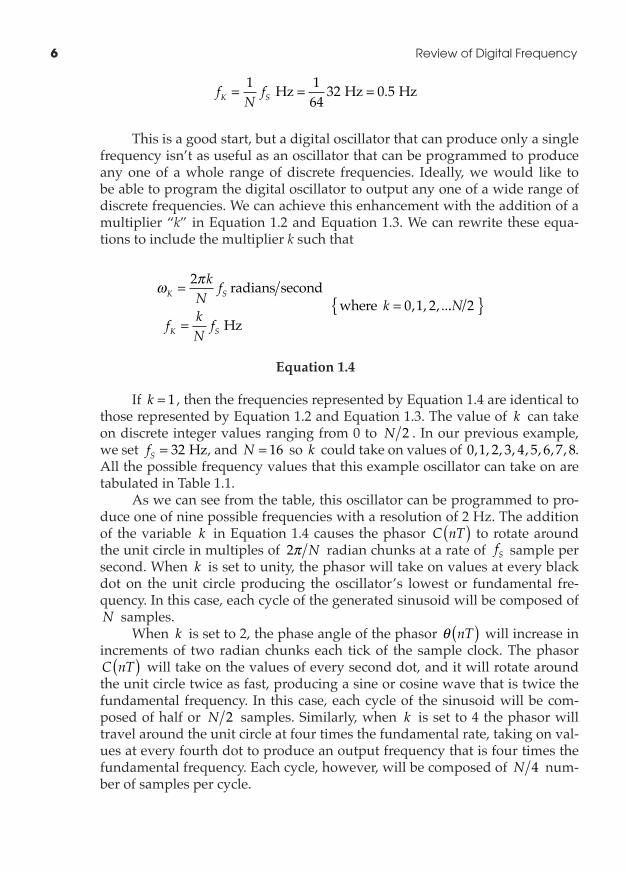
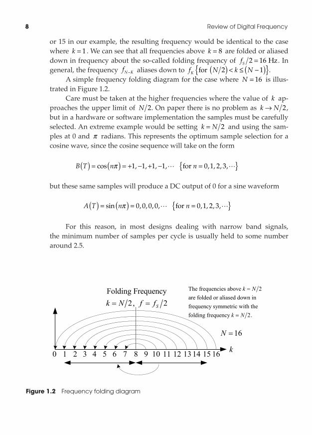
or 15 in our example, the resulting frequency would be identical to the case where k = 1 . We can see that all frequencies above k = 8 are folded or aliased down in frequency about the so-called folding frequency of fS 2 16= Hz . In general, the frequency fN K− aliases down to f N k NK for 2 1( ) < ≤ −( ){ }.
A simple frequency folding diagram for the case where N = 16 is illus-trated in Figure 1.2.
Care must be taken at the higher frequencies where the value of k ap-proaches the upper limit of N 2. On paper there is no problem as k N→ 2,but in a hardware or software implementation the samples must be carefully selected. An extreme example would be setting k N= 2 and using the sam-ples at 0 and π radians. This represents the optimum sample selection for a cosine wave, since the cosine sequence will take on the form
B T n n( ) = ( ) = + − + − ={ }cos , , , , , , , ,π 1 1 1 1 0 1 2 3 for
but these same samples will produce a DC output of 0 for a sine waveform
A T n n( ) = ( ) = ={ }sin , , , , , , , ,π 0 0 0 0 0 1 2 3 for
For this reason, in most designs dealing with narrow band signals, the minimum number of samples per cycle is usually held to some number around 2.5.
figure 1.2 Frequency�folding�diagram
0 1 2 3 4 65 7 8 9 10 11 1312 14 15 k
Folding Frequency2, 2Sk N f f
16N
The frequencies above 2are folded or aliased down infrequency symmetric with thefolding frequency 2.
k N
k N
16
1.3� Mathematical�Representation�of�Digital�Frequencies� 9
1.3 MatheMatiCal representatiOn Of Digital frequenCies
The notation in Equation 1.4 gives us a valid method to represent digital fre-quencies using a pencil and paper, but it doesn’t help us when it comes to the generation of a digital sinusoidal waveform in hardware or software. In Equation 1.4, we explicitly included the sample rate represented by the term fS . This is fine for mathematical computations on paper but the sample rate is
a fixed entity that is already implicit in the operation of the digital hardware. It does not make sense to include the fS term in frequency synthesis because it is already present due to the fact that each digital computation takes place at the sample rate.
In addition, Equation 1.4 provides us with a single value for any par-ticular frequency—something that we can write down on paper like the value 16 Hz or 48 Hz. This is not appropriate for the actual synthesis of a complete period of a sinusoidal frequency in hardware. In hardware or software, we need to generate all N samples of a sinusoid at the sample rate fS. To do that, we need to take into account the sample index n of the generated sinu-soid, and we need to normalize the sample frequency to 1. We normalize the frequency by dividing the frequency expression by fS. In doing so, we can rewrite Equation 1.4 to include these changes and produce
ω πK
K
n knN
f n knN
( ) =
( ) =
2 radians/second
Hz where
k Nn
== ∞
0 1 2 20 1 2 3, , ,, , , ,
Equation1.5
In Equation 1.5 we have normalized the sample frequency to 1. The nor-malized frequency of a digital waveform is usually expressed as a fraction given by k N. To convert a normalized frequency back to an unnormalized frequency, we simply multiply by the sample rate, or
f kNfK S=
Remember the sample rate is implicit in a hardware or software imple-mentation. It is the rate at which the computations are performed (i.e., the rate at which the phasor advances between black dots on the unit circle).
For example, if our sample frequency fS = 256 KHz , k = 16 , andN = 128, then the normalized frequency would be expressed as follows:
10� Review�of�Digital�Frequency
f k NK = = = 16 128 0 125. . The actual frequency in Hz can be determined by multiplying the fraction k N by the actual sample frequency fS or
f kNfK S= = ( )( ) = KHz KHz0 125 256 32.
The function of the sample index n in Equation 1.5 is to index succes-sive samples and to advance the phasor around the unit circle by acting as an incrementing multiplier to the fixed value k N . The term nk N can be thought of as an infinite series given by
kN
kN
kN
nkN
, , , , ,2 3
The correct way to generate a digital sinusoid waveform of unity magni-tude and normalized frequency k N is given by
A n kNn
B n kNn
( ) =
( ) =
sin
cos
2
2
π
π for
nk N
==
0 1 20 1 2 2
, , ,, , , ,
Equation1.6
It is important to remember that the term 2πN is a radian chunk. The
term 2πNk is a k multiple of a radian chunk. Since the sample rate is im-
plicit to the hardware and since we are dealing with normalized values of frequency, we can now drop the index notation nT as illustrated in Figure 1.1 and simply refer to the index as n as we did in Equation 1.5 and Equation 1.6. The phasor C n( ) will rotate around the unit circle at the sample clock rate in increments of 2πk N radian chunks. This means that the phasor sine and cosine components A n( ) and B n( ) will take on discrete values at each kth radian chunk and will do so at the clock rate.
Nothing is stopping us from writing down on a sheet of paper that the radian frequency associated with this radian chunk is 2πk N fS( ) , but keep in mind that this is just a number on a sheet of paper; it is not the sine or cosine argument that will trace out a sinusoidal waveform. This is where the sample index n comes into play. The index increments by one every sample clock so
1.3� Mathematical�Representation�of�Digital�Frequencies� 11
the argument 2πNnk takes on incremental k radian chunk values with each
clock period. This means that ω πK nk N= ( )2 will take on successive values of 0 2 4 6, , , ,π π πk N k N k N at the sample rate. This is the dynamic ar-gument of the sine and cosine function. If we plot A n( ) and B n( ) for this dynamic argument as n = 0 1 2 3, , , , , we will trace out a sine and a cosine waveform at the radian frequency 2πk N fS( ) .
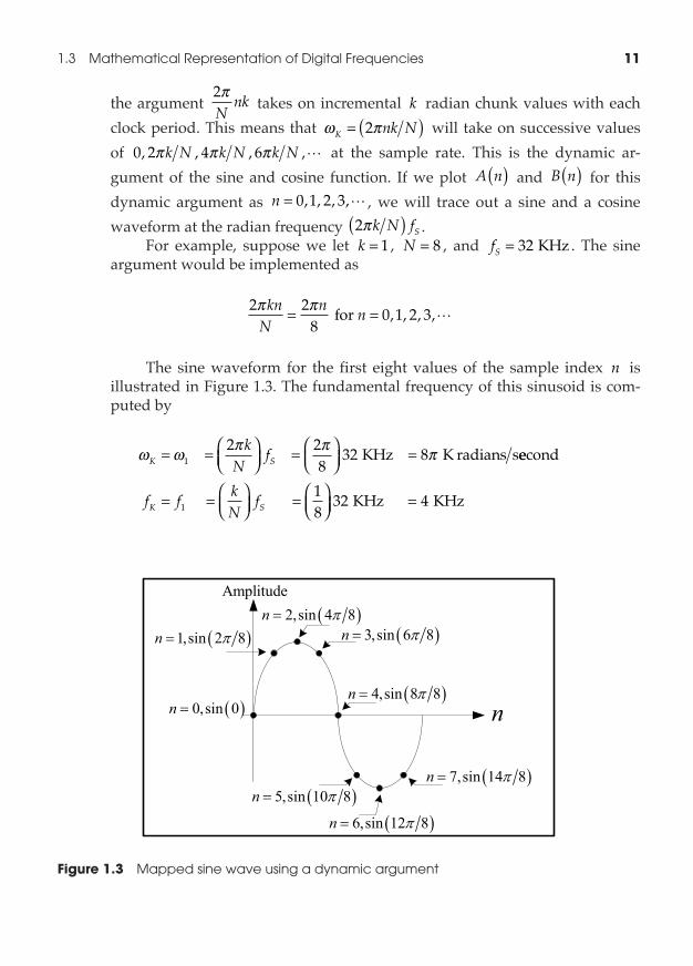
For example, suppose we let k = 1 , N = 8 , and fS = 32 KHz . The sine argument would be implemented as
2 28
0 1 2 3π πknN
n n= = for , , , ,
The sine waveform for the first eight values of the sample index n is illustrated in Figure 1.3. The fundamental frequency of this sinusoid is com-puted by
ω ω π π πK Sk
Nf= =
=
=12 2
832 8 KHz K radians seecond
KHz KHzf f kN
fK S= =
=
=118
32 4
figure 1.3 Mapped�sine�wave�using�a�dynamic�argument
0,sin 0n
1,sin 2 8n 2,sin 4 8n
3,sin 6 8n
4,sin 8 8n
5,sin 10 8n
6,sin 12 8n
7,sin 14 8n
n
Amplitude
12� Review�of�Digital�Frequency
The fundamental frequency is generated when k = 1. Multiples of the fundamental frequency are referred to as harmonic frequencies. Frequencies generated for k N= 2 3 4 2, , , , are harmonics of the fundamental. When the multiplier k = 0, we end up with a frequency of 0 Hz, or DC.
We can represent the phase offset in a digital sinusoid by the expression
sin 2 2 0 1π πknN
pN
p N+
= ≤ ≤ −Φ Φ where
The phase offset can only take on values equal to p radian chunks.When implementing a digital sinusoidal generator in hardware, it is of
paramount importance to remember the following seven points:
1. Since Equation 1.6 is computed every T seconds, it implicitly includes the sample rate term fS. This is because the index n increments at the sample rate.
2. In normalized notation, the frequency of the sinusoid in Equation 1.6 is given by the ratio of k N , where 0 0 5≤ ≤k N . .
3. The frequency resolution of the digital sinusoid waveforms A n( ) and B n( ) is determined by the size of N .
4. The phase resolution of the digital sinusoid waveforms A n( ) and B n( ) is determined by the size of N .
5. The precision of the amplitude of the sinusoidal waveform is determined by the bit width of the samples used to represent both A n( ) and B n( ).
6. The base or fundamental frequency of the sinusoids in Equation 1.6 is equal to 1 N normalized and f NS unnormalized.
7. The set of discrete frequencies that can be output by a programmable oscillator is given by k N for k N= 0 1 2 2, , , , , which equates to a nor-malized frequency range of 0 0 5 to . in steps of 1 N, or an actual fre-quency range of 0 2 Hz to HzfS in steps of f NS .
We will show in Chapter 8, “Digital Frequency Synthesis,” that the value of k in item 7 can take on fractional values, which allows the engineer to de-sign synthesizers that have much finer frequency resolution.
1.4 nOrMalizeD frequenCy
The notation in Equation 1.4 is based on the concept of dividing the unit circle into N equal arc segments. We can derive an equivalent expression simply by observing that the digital frequency
1.5� Representation�of�Digital�Frequencies� 13
f kNf k N
K S= ≤ ≤ where 02
can be normalized by dividing both sides of the equation by the sample fre-quency fS to arrive at
ff
kN
f f k NK
SK
S= ≤ ≤ ≤ ≤ where and 02
02
Equation1.7
Both sides of Equation 1.7 are now expressed as a fraction between 0 and 0 5. . We can drop the subscript K such that fK becomes f . When we do we can think of both f and fS as being two analog frequencies whose ratio just happens to be k N. This notation is useful if the unit circle is not specifi-cally considered in the derivation of digital frequencies. The two methods of notation are equivalent, as illustrated in Equation 1.8.
cos cos, , ,
2 20 1 2
π πffn k
Nn
n
S
=
= where
33ff
kNS
=
Equation1.8
It’s a matter of preference. Either notation is correct. This book uses both notations where appropriate.
1.5 representatiOn Of Digital frequenCies
A digital frequency can be written on paper in units of Hz or in units of radi-ans per second as
f kNf k
NfK S K S= = or ω π2
A more common method is to express a digital frequency as a fraction where the sampling frequency has been normalized to 1, such as
f kN
kNK K= = or ω π2
14� Review�of�Digital�Frequency
In all cases, the value of k can range from 0 to N 2. Examples of the four representations of digital frequencies are illustrated in Table 1.2 for sev-eral values of k .
A frequency in the analog domain has infinite resolution and therefore can take on all possible values. A frequency in the digital domain can only take on specific discrete values, which are multiples of f NS . The value of an analog frequency can always be made to match exactly the value of a digital frequency, but since the value of the digital frequency does not have infinite resolution, the opposite is not true.
The amplitude of an analog frequency can take on an infinite number of different values, whereas the amplitude of a digital frequency can only take on discrete values. The number of amplitude values that can be represented by a digital sinusoid is dependent on the bit width of the individual digital samples. For example, suppose the bit width of a bipolar sinusoidal sequence is given by B . The sinusoidal amplitude can take on values equal to 0 and ± −( )
−1 2 3 2 11, , , ,
B .The sole purpose of this chapter is to introduce the mathematical repre-
sentation of frequency in the digital domain. This book contains a great deal more information on the subject. For a detailed analysis and tutorial on the synthesis of digital frequencies the reader is encouraged to read Chapter 8, “Digital Frequency Synthesis.”
table 1.2 Four�Ways�to�Represent�a�Digital�Frequency
k = 0 k = 1 k = 2 k = N/2
Normalized radians ω π
kk
N= 2 0 2π
N4πN
π
Radians ω πk S
kN
f= 2 0 2πNfS
4πNfS
π fS
Normalized frequency f k
Nk = 0 1N
2N
0 5.
Frequency f kNfk S= 0 f
NS 2 f
NS
fS2
1093
A
acceptance test, 628address generation, 960– 961, 960faddress ramps, 581– 583, 609– 611, 615– 617
cycling and, 583, 610frequency of, 615least significant bits of, 641linear, 581look up tables, 581f, 581, 583, 589, 590,
609, 611t, 611, 643numerical clock oscillator design and,
581f, 610f, 625f, 625, 634, 634f, 638, 638f
offset, 638foutput, 615period of, 582, 595, 616phase accumulator, 582, 615, 616, 616f,
617, 617f, 643phase dithered, 643, 643fsample clock offset and, 617fwidth of, 582, 632
address space, 776circular memory, 813decision points and, 776DS- 1 bit stream generation, 809– 810variance, 776
alarm bit generators, 769, 802f, 803aliased region, 487faliased spectra, 193aliased zeroes, 521f
aliasing, 1, 7– 8, 192– 195, 204, 438– 439, 439f, 443– 445, 466, 468, 469f, 483– 490, 485f, 486f, 487f, 489f, 496– 498, 496– 498, 496f, 497f, 510, 514– 515, 519, 521– 523, 521f, 527– 536, 528– 529, 529– 536, 529f, 535f, 581, 955, 970
attenuation and, 496fbands, 496fdecimation and, 439f, 510tfirst edge, 497fimaging attenuation and, 497fimaging bands and, 483f, 485f, 486f, 487flevels, 487f, 521fnonaliased spectra, 439fpass band, 489t, 510t, 515e, 519f
alternating series test, 284amplitude, 2, 3, 11f, 174, 227, 235, 257,
875f, 903f, 905fanalog versus digital, 14, 630– 631Blackman window spectral main lobe,
246constant, 290discrete Fourier transform, 199– 200double sideband amplitude
modulation, 665Euler’s formula and, 215filtering, 386, 467, 451fluctuations, 378Fourier series and, 130, 136– 137, 139– 147,
141e, 143f, 144tfrequency response, 342, 425, 465
Index
Note: The letters f, e, and t indicate that the entry refers to a page’s figure, equation, or table, respectively.
1094� Index
amplitude (continued)fundamental frequencies and, 598growth and decay properties, 292Hamming window spectral main
lobe, 244harmonic frequencies and, 598identical, 654, 656, 717, 719impulse, 752– 753increasing, 323inverting, 668loop gain and, 1020main lobe, 241, 243maximum, 216, 243, 253f, 257, 583,
585– 586, 630modulation, 665, 979, 1020– 1022numerical clock oscillator phase offsets
and, 583– 486negative, 666, 732noise, 257– 258, 586overall system, 342pass band, 465plotting, 666, 667f, 669f, 707, 732f, 732pole location and, 339– 340precision of, 2, 12, 188pulse, 154, 159– 162real poles and, 292rectangular windowing and, 240, 253freducing, 630– 631response, 342, 465, 979, 980saw tooth waveforms and, 615sine waves and, 2, 12single- sided coefficients, 150– 151spectral line, 207spectral lines, 182spectrum, 171, 171e, 174– 175, 225, 243,
652, 666, 667f, 668, 669f, 729– 730spectrum for cos(2πf0t), 169espectrum of sin(2πf0t), 171esquare waveforms and, 596system response term, 480translating, 657, 664– 669, 667f, 669f,
729– 730, 734triangle wave, 155unity, 2, 213, 226, 752– 753voltage waveforms and, 182zero, 226, 338
analog AM radio receiver, 575analog capacitors, 363
analog signal processing, 1– 2, 13, 16, 187, 200, 595
amplitude of, 630analog- processing block, 970bandwidth, 972circuitry, 363, 970, 973– 974clipping of, 630continuous time Fourier transform, 235,
647– 688, 689, 692, 711conversion from digital, 7, 535– 536, 584,
630, 696, 970, 973conversion to digital, 7, 194– 195, 204,
355, 534, 535f, 596, 630, 878f, 879– 880, 970– 972, 971f
filters, 238frequency, 14– 15impulse response, 238input, 535f, 970narrow band, 194output, 535f, 820tsampling, 630spectrum analyzer, 371spectrum analyzers, 371telephone channels, 968time variable t, 582, 623tuning, 646undersampling, 7, 194wideband, 880f
analysis frequencies, 254, 255, 712, 881, 890, 1040
analytic functions, 41, 127, 329annular convergence ring, 282antennas, 646antialiasing, 194, 438, 534, 536, 970
filters, 438, 535fapplication- specific integrated circuits,
385– 386, 513, 633, 769, 774, 792, 961Applied Signal Technology, 873approximation errors, 394, 403, 424f, 425fapproximation expression, 488earc intervals, 29argument sequences, 950earithmetic logic unit, 540f, 543, 558, 558f,
559f, 577, 577f, 581f, 610f, 612f, 625, 625f, 634f, 637, 638f, 643f, 948, 949f, 959f, 962, 962f
arithmetic noise, 209attack rate, 826, 853, 978, 978automatic gain control, xx, 977– 1047
Index� 1095
amplitude response, 979f, 980fattack rate of, 978circuit parameters, 1030tcircuitry, 1033fDC signal response, 1000f, 1002f, 1005fdead band, 978– 979, 980fdecay rate, 978, 1015, 1045feedback coefficient, 988– 999, 990e,
991e, 993e, 995e, 1032– 1037, 1033f, 1034f, 1035f, 1036f, 1037f
initial response, 1017fnoise, 1037– 1044, 1037f, 1038e, 1039e,
1039f, 1040f, 1042f, 1043foutput signal RMS, 1010frelationship between output and input
signals, 987eroot mean square of signals, 1005fsimulations, 999– 1023, 1000f, 1002f,
1005f, 1006f, 1007f, 1008f, 1009f, 1010f, 1011f, 1012f, 1013f, 1014f, 1015f, 1016f, 1017f, 1019f, 1022f, 1032– 1037
transient response, 979f, 980f, 1005f, 1015f, 1023– 1032, 1023e, 1024e, 1026e, 1026f, 1027e, 1030t, 1031e, 1031f, 1032f, 1033f
Type I RMS AGC Circuit, 979f, 981– 1044, 981e, 982f, 984f, 985e, 986f, 987f, 988f, 990e, 991e, 993e
Type II RMS AGC Circuit, 980f, 1044– 1047, 1045f, 1046f
B
band limited signals, 172, 177, 529– 646, 657– 658
analog, 877discrete Fourier transform bin, 910discrete Fourier transform filter, 895input message signal, 661multiplication, 174– 175spectral inversion of, 195spectrum, 740
band of interest, 194– 195, 468– 469, 482– 488, 483f, 485f, 486f, 487f, 498, 520f, 527, 528, 529f, 533
band pass filters, 403t, 411e, 417t, 423t, 426t, 427t, 432t, 565t, 687f, 878– 884, 883f, 899f, 914– 918
adjacent, 899fbanks of, 905fdiscrete Fourier transform summation
bank, 894fenhanced discrete Fourier transform,
905ffilter response, 905foverlap, 224Parks- McClellan routine output, 411espectral leakage from, 899f
bandslower sideband, 666, 731, 731f, 874,
875f, 879mirror image spectral, 740upper sideband, 665, 665f, 731, 731f,
874, 875fbase band, 194, 204, 219, 482– 485, 518,
520, 522– 525, 528, 535, 541, 567, 575, 608, 645– 646, 645, 657, 669, 672, 679– 680, 685, 687, 738, 744, 873, 895, 902, 964, 970
Bell Laboratories, 245binary points, 609– 610, 609f, 612, 612f,
634– 635, 638, 643, 643fbit accumulation, 774, 776– 777bit generators, 802– 803, 802fbit location, 768, 770, 782– 783, 795– 796,
803cascaded integrator comb decimators,
501t, 503e, 504e, 505eexample, 502tHogenauer LSB procedure, 499– 500Hogenauer LSB procedure, 517
bit rate, 764, 766– 769, 774– 782, 784, 804, 829, 869, 879, 973
data stream, 766, 768elastic store memory, 771– 774, 771tmodifying, 768
bit variance, 777, 779bit width, 2
cascaded integrator comb, 511terror signal, 843t, 866tminimal, 359of digital errors, 843tregister, 511tregister, 517t
bitsdo not insert information, 777ffill, 768
1096� Index
bits (continued)garbage, 768information, 768insert information bits, 775finsert information bits, 777fleast significant bits, 372, 501– 502, 501t,
503e, 504e, 505e, 825noninformation, 768register bit width, 355, 356stuff or garbage, 766, 768f, 768, 770ftruncated, 499
Blackman, Ralph Beebe, 245block diagrams, 204f, 317
channelizers, 880f, 962fcomplex signal translation, 746f, 748fconverting complex signals to real, 540fdecimate by two filter, 446fdecimation, 446fDS- 1C multiplexer, 802felastic store memory, 793ffolding memory, 926ffrequency division multiplex signal
extraction, 687fnumerically controlled oscillator, 577f,
581f, 610f, 625f, 634f, 638f, 643fphase offset, 638fsimplified demultiplexer, 808fspectral inversion control, 942ftranslation by ej 20pt t, 677ftranslation of a complex signal, 680ftypical signal processing system, 535f
Brigham, Oran, 268buffers
double, 923f, 925finput memory, 923f, 925f, 928f, 962fsplit, 959f, 960fsplit addresses, 961t
C
carrier signals, 664, 979cascaded integrator comb filters, 435,
470– 531bit pruning, 499– 506, 501t, 503e, 503e,
505ecleanup filter, 526– 531comb filter stage, 471– 473composite, 473
composite filter z- transform, 475– 477decimation filter, 477– 478, 483, 499– 506,
514– 523, 515t, 516f, 517t, 518f, 519f, 520f, 521f, 527– 528, 529f
filter gain, 498filter response, 473frequency response, 473impulse response, 491– 492integrator stage, 474– 475interpolation filter, 478– 479, 506– 514,
508, 511t, 523– 526, 524f, 528– 531, 530fpass band droop, 506– 508phase response, 490– 491pole- zero placement, 493– 498sample rate frequency response, 479– 490
Cauchy, Augustin- Louis, 111Cauchy- Riemann conditions, 42, 47– 51,
48t, 49tCauchy’s theorem, 96– 108, 98f, 102f, 105f,
109– 120, 111e, 113e, 121eceiling line, 53, 53f, 62center frequency, 261– 262, 537, 621– 622,
645, 664– 665, 681, 729, 730, 809, 822– 824, 845, 847, 854– 855, 855
constant increments of, 684converting to, 194, 262deviation from, 869, 857f, 858ffilter response, 563generate, 822image bands, 525loop, 862max variance, 845normalized, 935normalized bin, 712output, 823point, 847pull range, 822sequential discrete Fourier transform
bins, 895simulations of, 866specifying, 822temperature, 614tuning signal, 675, 743, 744variance, 845voltage controlled crystal oscillator,
823– 824, 829– 831, 845– 850, 869wideband frequency division multiplex
signal, 892channelized filter banks, xx, 873– 975, 974e
Index� 1097
block diagrams, 958– 962, 959f, 960e, 960f, 961t, 962f
design of, 919– 962, 967– 974equations for, 974– 975function of, 877– 919hardware, 967– 974, 968f, 969f, 970f, 971fsoftware simulation results, 962– 967,
963f, 965t, 966f, 967fchannelizers, 873– 879, 875f, 876f, 878f,
880f, 958fcomplex to real conversion, xviii, 942–
948, 943e, 944e, 945e, 946e, 947f, 948tcosine look up tables, 948– 955, 949e,
949f, 950e, 950t, 951e, 951t, 952e, 953t, 954t, 955f
data, 942fdata processing, 907– 910, 909fdiscrete Fourier transform, 881– 900,
881e, 883f, 884e, 885f, 887e, 887f, 889f, 890e, 890f, 891f, 892f, 893f, 894e, 894f, 896f, 898f, 899f, 913e
functional, 880fhardware design, 971fimplementation, 873input signal processing, 919– 923, 920t,
921f, 923f, 930– 930, 930e, 931e, 931finput test signal, 963fmathematical concepts, 910– 919, 911e,
911f, 912f, 913e, 915e, 916e, 917e, 918eoperational parameters, 919sample rate decimation, 932– 933segment folding memory, 923– 930, 924e,
925f, 926f, 927f, 928e, 928f, 929e, 930esoftware simulation design parameters,
965tstand- alone, 945e, 974etime varying phase terms, 933– 942,
933e, 934e, 936e, 937e, 938f, 939e, 940e, 941e, 942f
channels, 646bandwith, 684f, 685fchannel stack, 537– 538, 874, 972– 973identity tones, 966f, 967f, 968f, 969f, 970freference tone, 615, 964– 965, 966f, 967f,
968f, 969f, 970fcircuitry
analog, 970, 973– 974analog- processing block, 970attack rate of, 978
board geometry, 237calculating time constant k, 854decay rate, 978, 1015, 1045feedback coefficient, 985fixed parameters, 839frequency response, 376layout, 237load, 238loop gain, 987eLSI 16- by- 16- bit multiplier chips, 431macros, 238scale factor, 985small scale integrated circuits, 237
circular memory, 761f, 794– 796, 794f, 797f, 798f, 799, 800f, 811, 813, 814f, 816f, 817, 825, 835
clock jitter, 825– 826, 828, 844, 851, 852f, 854, 855f, 857f, 857f, 857f, 857f, 857f, 858f, 859f
clock oscillators, 455f, 456f, 613– 637, 761, 768, 790, 820, 827, 859
clock teeth, 809, 814clock tree skew, 238code
converter code glitches, 534length, 642snippets, 788, 947, 1058, 1060, 1083
coefficient memory, 389, 456, 457f, 461, 925f, 928f, 962f
coefficients, 388edouble- precision, 404, 564filter, 904floating point, 564sliding filter vectors, 548
coherent integration method, 260– 261comparison tests, 284complementary metal- oxide
semiconductor devices, 237– 238complex numbers, 17– 37, 38f, 39f
absolute value of, 35– 36addition, 18eCartesian form of, 17– 21, 18f, 18e, 19e,
20e, 21econjugates, 19e, 20e, 21econverting Cartesian and polar
forms, 23econverting to polar form, 106– 107
1098� Index
complex numbers (continued)division, 18e, 24edot product, 27fequality, 18e, 23eexponential form of, 36– 37graphs of, 38f, 39fmagnitude, 19emultiplication, 18emultiplication, 23epolar form of, 21– 27, 21e, 22e, 22f, 23e,
24e, 25e, 26epowers of, 25e, 26eproperties of, 18– 21, 18e, 23– 27real numbers versus, 16representation of, 271– 274roots of, 27– 34, 27e, 28e, 29e, 31f, 33f, 34f
complex variables, 15– 127, 272fanalytic functions, 41– 42Cauchy- Riemann equations, 47– 51Cauchy’s theorem, 96– 108, 109– 120complex differentiation and, 43– 46contours, 51entire functions, 42limits and, 40– 41line integrals, 51– 54, 84– 96real line integrals, 54– 84residue theory and, 120– 127simply connected regions, 51
componentsaging, 614, 618, 637alternating current, 863– 864direct current components, 863– 864in- phase, 16– 17quadrature, 16– 17real versus imaginary, 92scalable libraries, 386
conjugate pairs, 342– 344, 367constant group delay, 385, 387, 470,
490– 491constant phase delay, 387contours
Cauchy’s theorem, 98f, 102f, 105fcircular, 64– 65, 81fclosed, 51, 54equivalent, 117fexamples of, 51f, 56f, 67fintegral, 52– 53, 53fintegral summation curtain, 53fintegration, 55
line integrals and, 52singularities and, 99ftriangular, 62
control bus interface, 793fCooley, J. W., 267Cooley- Tukey FFT algorithm, 268copper wire, 646, 678, 762, 874, 973core memory, 632
D
D flip- flop, 614, 769, 792, 794, 803data
aligning, 911fblocks, 911, 923f, 926, 933channelized, 942fchannelizer processing paths, 909fdiscrete Fourier transform channel
outputs, 939e, 940edriver source current, 801example data transmission frame, 790fmultiplying, 911fservice level, 764shifted, 549f, 551f, 553f, 557f, 558f,
559f, 939esimulation, 567– 573, 568f, 571f, 572fsynchronous, 968throttling, 772, 779tributary data bit streams, 802f
data locked loops, xix, 807– 871, 808f, 808f, 869e, 869e, 870e, 871e
analog error voltage, 818– 820, 819f, 820tcircular memory and, 814fclock frequency synthesis, 820– 825,
821f, 824telastic store memory and, 804, 809– 817,
812f, 813f, 814f, 816f, 810ferror signal bit width versus time
constant, 843terror signals, 817error voltage generation, 819ffill, 813ffrequency devation and, 867ffrequency response and, 827f, 828fmodulo operation, 814foperational characteristics, 825– 829,
827f, 828fread pointers, 812f, 816f
Index� 1099
reference clock synthesis, 821frise time, 861, 862f, 865e, 866tsimulation, 844– 868, 846f, 848t, 849f,
852f, 853f, 855f, 857f, 858f, 859f, 860f, 862f, 864f, 865e, 866e, 866t, 867f
steady state behavior, 829– 834, 829e, 830e, 830f, 831f, 832e, 832f, 866– 868, 866e, 867f
transient behavior, 834– 844, 836e, 837e, 838e, 839e, 840e, 841e, 842e, 843t, 838e, 839e, 861– 866, 862f, 864f, 865e, 866t, 812f, 816f
decimation, 436, 437– 448, 437f, 438f, 439f, 440e, 440f, 441e, 442f, 443f, 444e, 445f, 446f, 447f, 448f, 521f
block diagram, 443f, 446fdecimate by two filter, 445f, 446f, 466factor, 777ffiltering, 535f, 1045fmagnitude, 539fpoly phase filters and, 443fratio, 909fsample rate, 496f, 529f, 539f
derivatives, 44– 45design review, 422, 509, 514, 545– 546, 559,
621, 628, 1021digital capacitors, 363“digital radio,” 528, 533, 535, 646, 677digital signal processing systems, xiii– xv
complex, 533– 570conversion from analog, 7, 194– 195,
204, 534, 535f, 596, 630, 878f, 879– 880, 970– 972, 971f
conversion to analog, 535– 536, 584, 630, 696, 970, 973
converting complex to real signals, 560– 573
real, 533– 570simulating, 560– 573tuning, 645– 759typical, 534– 540
digital signals, 1– 14defining, 2– 8, 3f, 4e, 5e, 6e, 7tdiscrete values, 4, 14errors, 613– 622mathematical representations of, 9– 12,
9e, 10e, 14trepresentations of, 9– 12, 13– 14
standard implementation representation of, 691e
synthesizers, 535f, 575– 644direct current, 139direct current components, 863– 864
canceling circuit, 376removal circuit, 379fsteady state behavior, 863– 864
Dirichlet conditions, 130discrete Fourier transform, 187– 253,
880f, 906fadjacent bins, 246, 714Bartlett windowing, 241– 243, 242e, 242fbin band pass filters, 218– 220Blackman window, 245– 246, 245e,
246f, 251fchannelizer discrete Fourier transform
output, 913e, 915e, 917e, 918ecomplex output points, 206discrete power spectrum, 211– 212,
212e, 213eenhanced filter, 956f, 957fexample application using, 261– 263filter banks and, 907filter response, 931ffinite impulse response filter window,
246, 247e, 248fforward, 209e, 210efrequency, 189– 195frequency bins and, 249fHamming window, 243– 244, 244e,
244f, 245fHanning window, 243, 243e, 252fincreasing processing gain, 260einherent frequency response, 974einverse, 209– 210, 209e, 210e, 647e,
650e, 933eL points, 880, 881e, 883f, 906fleakage, 220– 236pairs, 218, 219tpoly phase enhanced, 902f, 903fpreprocessors, 237processing gain, 254– 261, 255eprocessing number of cycles with,
234f, 236fproperties, 217, 218tpulse waveforms, 213– 217rectagular window, 238– 241, 239e, 239f,
240e, 241f, 250f, 252f
1100� Index
discrete Fourier transform (continued)representation, 210– 211resolution, 209scale factors and, 210eshifted input data and, 939estandard display conventions, 519summation filters, 884, 893f, 894f, 898fsymmetry, 195– 209system interpretation of, 896ftime, 263– 267, 264ewindowing, 236– 253, 253t
“do not insert information” bits, 775f, 777fdot products, 26– 27, 27f, 384, 440– 441,
458, 547– 549, 552, 557double precision array, 396t, 1059double sideband amplitude modulation, 665down conversion, 645, 685
frequency division multiplex signal, 685fdown sampling, 436– 438, 463, 478, 516Drichlet conditions, 130dual inline packages, 637duty cycles, 140– 142, 141t, 143f, 144f, 144t,
614, 809, 814, 974dynamic arguments, 11f
E
elastic store memory, xix, 761– 805, 780tbit accumulation levels, 774, 776– 777block diagram, 793fbrute force implementation, 775– 776,
775fconceptual, 794fdata locked loops and, 804, 810fdata rates, 770– 774, 771tdepth, 843tdesigning, 769– 770, 774– 777DS- 1C multiplexer design, 768– 774,
801– 803, 802fefficient, 776– 777, 777fexample application, 762– 763fill, 779, 793f, 797f, 798f, 800f, 802fhardware implementation of, 792– 801,
793f, 794f, 797f, 798f, 800flimits, 779North American Digital Hierarchy, 765–
768, 766t, 768foutput bit rate, 771t
pulse code modulation multiplexing hierarchy, 763– 768, 764t
read bit rate, 771tsimulation, 778– 779, 788– 791, 790fsize, 774– 775software implementation of, 788– 791steady state, 779– 783, 780t, 782t, 783tthreshold value, 793ftransient statistics, 784– 791, 785t, 787t
energy spectral density, 185– 186, 185eequations
Cauchy- Riemann equations, 47– 51Cauchy- Riemann equations in polar
form, 50channelized filter banks, 974– 975digital data locked loops, 869– 871plug- in, 350pole, 334– 350signal tuning, 754– 759zero standard form, 334– 350
errorsdecay, 856design specific loop digital error signal,
829eerror accumulation, 856frequency error bounds, 620finitial, 1016floop, 1003, 1005floop digital error signals, 829emaximum, 418MDAC voltage to error relationship, 830eperiodicity of, 602predefined error bounds, 157rounding, 600, 601f, 602f, 605f, 639fscaled feedback signal, 985etruncation, 597f, 598fvoltage generation, 819f, 821fvoltage response and, 849fzero error operating point, 832f
Euler’s equation, 167, 188, 188e, 215, 266, 306, 306e, 307, 322, 337, 344, 480, 653, 655, 683, 686, 702, 706, 713, 716, 718
European or CEPT Digital Hierarchy, 763
F
factorization, 126, 312fast edge rate clocks, 801
Index� 1101
fast Fourier transform, 267– 268fill bit, 768fill difference, 793f, 794f, 795, 797f, 798f,
800f, 812, 813f, 814f, 816fadjacent filters, 899fanalog, 238antialiasing, 194, 438, 534, 535f, 536, 970anti- imaging, 449banks of, 894f, 905f, 907cascade, 428, 463, 467– 468, 527– 530clean up, 469f, 514, 523, 529f, 530fcoefficient memory, 962fcoefficients, 388, 565t, 904, 925f, 928fcomposite, 906fdecimate by two, 445f, 446fdecimation, 436, 535f, 1045fdesign, 392– 425direct form, 384, 427discrete Fourier transform filters,
220, 907enhanced discrete Fourier transform
filter, 905f, 931fexamples of, 370tfinite impulse response, 383– 531four- phase, 447half band filters, 425– 433implementation of, 425– 433length, 423t, 426t, 427t, 432t, 441,
565t, 906fmultirate filters, 435– 531overlap, 224parallel filter structures, 328poly phase filters, 436– 465recursive, 364, 371f, 372fsimulations of, 566f, 567fsliding coefficient vectors, 548summation, 884, 887f, 888ftransition bands, 904transversal architecture, 427two- filter cascade, 463two- phase, 443
finite impulse response filters, xvii– xviii, 383– 531, 403t, 417t, 423t, 426t, 427t, 432t, 565t
architecture, 546fcascaded integrator comb filters, 470– 531clean up filters, 529f, 530fdesign, 392– 425direct form, 384
direct form architecture, 389– 392discrete time differences and, 384eeven coefficient architecture, 389– 390filter types, 387– 389half band filters, 425– 433linear phase, 386– 387, 388e, 389– 392low pass digital, 393multirate, 435– 531odd coefficient architecture, 390– 392Parks- McClellan design method, 392– 425poly phase filters, 436– 465shorthand drawing notation for, 547ftransfer function, 385ewindowing, 248f
flash memory, 581flip- flop, 614, 769, 792, 794, 803floating point, 586, 592, 632, 641, 1009, 1050
attenuation of, 417double- precision, 401, 403, 408, 410,
414, 417, 421– 422, 430, 564, 956filter coefficients and, 408, 422Microsoft Excel, 209Parks- McClellan FOTRAN subroutine,
1057– 1060, 1065, 1084t, 1090processors, 404samples, 596system, 379
fold and sum operation, 924, 925f, 948folding frequencies, 192, 437, 487f, 496f,
497f, 519f, 519, 521ffolding memory, 923– 924, 926, 946– 947,
948– 949, 948t, 949f, 958– 961, 962fblock diagram, 926fcomputational example, 927fdouble buffers and, 928finversion term, 947fmodified architecture, 949fsplit buffer, 959f
follow on system, 372, 435forward Fourier transform, 647, 647eFourier series, 129– 157, 137f, 140e
coefficients, 153compact form of, 148ecomputed, 153graphs of, 143f, 149f, 153fharmonics of, 141t, 144t, 148tharmonics of, 157one sided, 153, 153fParseval’s theorem, 181
1102� Index
Fourier series (continued)single- sided, 150etrigonometric, 130e, 131e, 132e, 133e,
135e, 139etwo- sided, 153f
Fourier transform, xvii, 129– 269, 380econtinuous, 180t, 181t, 647– 688discrete Fourier transform, 263discrete time (digital), 187– 253, 188e,
191e, 201, 203f, 205e, 254– 261, 261– 267, 689– 754
fast Fourier transform, 267– 268forward, 158e, 159eFourier series, 129– 157graphs of, 201, 202finverse, 158e, 159epairs, 164e, 165e, 166e, 167e, 180t, 649e,
650e, 651eproperties, 179, 181ttime sequences and, 274eunit circle of, 201zoom, 435z- transform and, 274e
frames, 766, 876fDS- 1, 766texample data transmission, 790fframe alignment, 766, 802fhalf, 772master, 768fmicroframes, 767, 768f, 780tpulse synchronizers, 363subframes, 766, 768
frequencyaliasing, 1, 7– 8, 192– 195, 204, 438– 439,
439f, 443– 444, 443– 445, 466, 468, 469f, 483– 490, 485f, 486f, 487f, 489f, 496– 498, 496f, 497f, 510, 514– 515, 519, 521– 523, 521f, 527– 536, 528– 529, 529– 536, 529f, 535f, 581, 955, 970
aliasing tree diagram, 194faxis folding, 192f, 193fcutoff, 430ffolding, 8, 8f, 192, 192, 193f, 438, 467,
484, 486f, 487f, 496f, 497f, 519f, 521fgraphs of, 192f, 193finput tributary bit clock, 848tnormalized, 9– 10, 12, 192, 211, 217,
225– 227, 234– 235, 239, 249, 250f, 251f, 252f, 258f, 266– 267, 362, 389, 393, 396t,
396, 399, 405– 406, 412, 419, 488– 489, 534– 536, 538, 539– 540, 560, 561f, 563– 564, 566f, 567f, 567, 570, 571f, 690– 714, 717e, 889– 892, 1007– 1008, 1013, 1037
Nyquist, 7, 191, 438, 701f, 704f, 708f, 709f, 718f, 720f
optimal, 590, 604possible values, 6radian, 2, 4– 5, 10– 11, 158– 159, 161, 182,
188– 189, 239, 253t, 266, 338f, 339f, 341f, 343f, 347f, 349f, 371f, 372f, 372, 375f, 377f, 378f, 648, 690– 692, 712, 754e, 755e, 888– 889, 892
resolution, 2, 12, 191– 192, 232– 233, 233– 234, 240, 243, 264, 268, 435, 579, 586, 604, 608– 609, 611– 613, 632– 633, 633, 826, 828, 833, 842– 844, 851– 854, 856– 858
step changes, 844step downs, 849funnormalized, 224voltage controlled crystal oscillator,
832ffrequency axis
calibration of, 201folding, 193
frequency deviation, 845, 849f, 851, 852f, 853f, 855f, 857f, 858f, 859f, 860f, 867f, 869
frequency division multiplex processing system, 448, 535, 645– 646, 679– 680, 684– 685, 878f, 892, 940, 957– 958, 964, 966– 970, 972
block diagram, 687fchannels, 535channels, 875fdown conversion, 685fsignal extraction, 687fsignal spectra, 684f, 878ftime division multiplex conversion,
873– 881time division multiplex signal
pathway, 878ffrequency impulse, 221, 570, 668, 671– 672,
675, 678, 738, 743, 747, 752, 891cancellation, 656cosine, 664, 714, 729function, 165, 650response, 167
Index� 1103
shifted, 650, 650esuperimposed, 895
frequency inversion phenomenon, 938frequency jitter, 825, 860ffrequency offset, 848t
output versus voltage controlled crystal oscillator control voltage, 824t
unwanted, 615zero, 620f
frequency rejection, 572ffrequency sampling method, 384frequency shift keyed communications
system, 576fundamental frequency, 4, 6, 11f, 190, 595t,
612f, 634f, 638fdirect current components, 130, 142harmonics in relation to, 12, 136, 140numerically controlled oscillators,
579– 580, 584– 585, 587– 588, 594– 595, 598, 608, 611, 613, 615, 632– 634, 638
G
gallium arsenide gate arrays, 238, 800garbage (stuff) bits, 768f, 770, 776, 779, 802generic base band signal spectrum, 518graphical user interface, 395Green’s theorem, 79– 84, 79e, 80f, 87, 90, 97ground bounce, 237grounding techniques, 373group delay, 386eguard bands, 777, 792, 833– 834,
964– 965, 973
H
half band filter, 425, 435, 469ffrequency response, 469fParks- McClellan routine output, 432t
half frame, 772Hamming, Richard Wesley, 243hardware
channelizers, 971fdigital sinusoidal generators, 12elastic store memory and, 792– 801follow on, 372, 435hardware multipliers, 546implementation, 12
pole- zero plot of, 297frecursive structure, 295fspecial purpose digital, 237
harmonic frequencies, 12, 595tfundamental frequencies and, 130odd, 598
headroom, 801heap memory, 632heterodyne, 573hexadecimal format, 588, 634Hilbert transforms, 389, 396e, 1067,
1072, 1087histogram, 533Hogenauer, E. B., 470– 471, 488, 512Hogenauer LSB pruning procedure,
499, 517
I
identity tones, 966f, 967f, 968f, 969f, 970fimage bands, 512f, 568f
aliasing and, 483f, 485f, 486f, 487fanti- imaging low pass filter, 449attenuation, 510t, 515e, 568ffirst edge, 497finterpolate by two, 542fresidue, 530f
image rejection, 512f, 572f, 932integers, 396eintegral test, 284integrals
arc length of, 67f, 68e, 69fcommon, 110tcomplex, 110tcomplex line, 84e, 87e, 90econtour, 73edefinite, 52, 52f, 53f, 91double, 79evaluating, 108eexamples of, 57e, 57f, 58e, 59f, 61f,
63f, 65fparametric forms of, 70epath independent, 91e
integrationattenuation, 363tfrequency response, 362fgain, 260graphs of, 92f, 95f
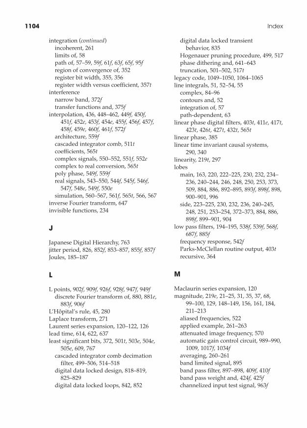
1104� Index
integration (continued)incoherent, 261limits of, 58path of, 57– 59, 59f, 61f, 63f, 65f, 95fregion of convergence of, 352register bit width, 355, 356register width versus coefficient, 357t
interferencenarrow band, 372ftransfer functions and, 375f
interpolation, 436, 448– 462, 449f, 450f, 451f, 452e, 453f, 454e, 455f, 456f, 457f, 458f, 459e, 460f, 461f, 572f
architecture, 559fcascaded integrator comb, 511tcoefficients, 565tcomplex signals, 550– 552, 551f, 552ecomplex to real conversion, 565tpoly phase, 549f, 559freal signals, 543– 550, 544f, 545f, 546f,
547f, 548e, 549f, 550esimulation, 560– 567, 561f, 565t, 566, 567
inverse Fourier transform, 647invisible functions, 234
J
Japanese Digital Hierarchy, 763jitter period, 826, 852f, 853– 857, 855f, 857fJoules, 185– 187
L
L points, 902f, 909f, 926f, 928f, 947f, 949fdiscrete Fourier transform of, 880, 881e,
883f, 906fL’Hôpital’s rule, 45, 280Laplace transform, 271Laurent series expansion, 120– 122, 126lead time, 614, 622, 637least significant bits, 372, 501t, 503e, 504e,
505e, 609, 767cascaded integrator comb decimation
filter, 499– 506, 514– 518digital data locked design, 818– 819,
825– 829digital data locked loops, 842, 852
digital data locked transient behavior, 835
Hogenauer pruning procedure, 499, 517phase dithering and, 641– 643truncation, 501– 502, 517t
legacy code, 1049– 1050, 1064– 1065line integrals, 51, 52– 54, 55
complex, 84– 96contours and, 52integration of, 57path- dependent, 63
linear phase digital filters, 403t, 411e, 417t, 423t, 426t, 427t, 432t, 565t
linear phase, 385linear time invariant causal systems,
290, 340linearity, 219t, 297lobes
main, 163, 220, 222– 225, 230, 232, 234– 236, 240– 244, 246, 248, 250, 253, 373, 509, 884, 886, 892– 895, 893f, 898f, 898, 900– 901, 996
side, 223– 225, 230, 232, 236, 240– 245, 248, 251, 253– 254, 372– 373, 884, 886, 898f, 899– 901, 904
low pass filters, 194– 195, 538f, 539f, 568f, 687f, 885f
frequency response, 542fParks- McClellan routine output, 403trecursive, 364
M
Maclaurin series expansion, 120magnitude, 219e, 21– 25, 31, 35, 37, 68,
99– 100, 129, 148– 149, 156, 161, 184, 211– 213
aliased frequencies, 522applied example, 261– 263attenuated image frequency, 570automatic gain control circuit, 989– 990,
1009, 1017f, 1034faveraging, 260– 261band limited signal, 895band pass filter, 897– 898, 409f, 410fband pass weight and, 424f, 425fchannelized input test signal, 963f
Index� 1105
channelizer data processing paths and, 909f
clock jitter and, 851– 860complex pole, 364complex variable z, 272– 273computing, 266, 345, 361, 374, 1070,
1073– 1074cursor measurements and, 415f, 416f,
422fdigital data locked operations and,
825– 829discrete Fourier transform, 200, 210,
215– 217, 220– 221, 882– 884, 1039– 1041discrete Fourier transform filtering,
956f, 957ferror signals, 825, 984, 987, 995, 1009fill, 819f, 821ffilter lobes, 223– 224, 234– 236, 240– 244,
254, 886filter response, 232– 233finite impulse response filters and, 386first order complex conjugate poles,
322– 324, 323f, 324ffloating point sinusoid, 596frequency discontinuity, 251frequency response, 222, 334– 342,
346– 347, 349– 350, 365– 366, 386half band filtering, 431fharmonic components and, 599high pass filtering and, 415f, 416fhigh sample rates and, 480infinite, 347input, 355, 895integrator frequency response, 361interpolation filter stop band, 570, 573left- sided sequence, 280– 281log, 595low pass filtering, 402fmaximum, 482, 594, 993noise, 255– 260output, 235, 371, 903, 966f, 968f, 969f,
970f, 984, 987, 995, 1039– 1041pass band ripples and, 396– 397peak, 240phase response and, 480reducing, 1035region of convergence and, 296– 297residual image, 573right- sided sequences, 280, 284– 285
round off error, 600signal discontinuity, 241signal energy, 225spectral leakage, 222– 224, 234, 242, 251spectrum of complex signals, 541square waveforms and, 599stabilizing, 825stop band filtering and, 421f, 422fsystem stability and, 290truncated sinusoid sample, 596two- sided sequence, 282uniform, 649, 694unity, 2, 10, 222, 234, 473, 692windowing and, 251, 253tzero, 222, 347, 370t, 964
McClellan, James H., 392microcontroller command, 642microprocessor bus, 577Microsoft Excel, 208– 209, 221, 227, 228f,
322, 338, 340, 341f, 342, 343f, 347, 349, 350, 365– 367, 369, 374, 490, 508, 952, 992, 1029, 1032, 1033f
Microsoft FORTRAN Power Station 4.0 compiler, 1063
Microsoft Visual C++ 6.0 Professional compiler, 1063
mixed language programming, xx, 1049– 1090
array arguments, 1059– 1060C/C++ main program, 1051, 1083– 1090,
1084tcalling subroutines and functions,
1051– 1054compiling, 1063– 1064, 1090floating point arguments, 1057– 1058FORTRAN functions, 1055FORTRAN subroutines, 1054– 1055integer arguments, 1055– 1057Parks- McClellan Fortran subroutine,
1064– 1082pointer arguments, 1060– 1063
multiplexing, 443, 688, 802f, 808f, 880fasynchronous input tributaries, 763– 764DS- 1C multiplex elastic store
memory, 766functional DS- 0 to DS- 1C, 765finput, 448time division signals, 878f
multiply/accumulate operations, 444

1106� Index
multiplying D/A converter, 818, 819f, 821fanalog voltage controlled crystal
oscillator control voltage, 824tbipolar configuration, 820tdigital input words, 824tunipolar configuration, 820tvoltage controlled crystal oscillator
control voltage, 824tvoltage reference pin, 822voltage to error relationship, 830e
N
noiseadditive, 1043farithmetic, 209floor level, 252, 262loop errors and, 1043fmagnitude, 255maximum amplitude, 1038enarrow band, 254noiseless input, 1043frandom, 255
noninformation bit, 768nonlinearity, 822, 834nonzero, 152North American Digital Hierarchy, 763,
764t, 765– 768, 765f, 766f, 768fnumerically controlled oscillators, xviii,
575– 644accumulator offset and, 577fblock diagrams, 577f, 581f, 610f, 625f,
634f, 638f, 643fdesign performance, 638– 641, 639f, 640fdesigning, 628– 640enhanced phase accumulators, 608– 613frequency errors from, 613– 622frequency resolution of, 579, 586, 608–
609, 611– 613, 633harmonics, 595tindustry- grade, 628– 640, 629e, 630eoperation of, 629eoutput, 589f, 591f, 613– 622, 620f, 622–
628, 626f, 635t, 639f, 640fphase accumulator, 577– 581, 577f, 579e,
580e, 601, 608– 613, 609f, 610f, 611t, 612f
phase dither, 641– 644, 642e, 642f, 643f, 643t
phase offset, 622– 628, 622e, 624e, 625e, 625f, 626f, 627f, 628f, 637– 638, 638f, 640f
phase register, 575– 577, 609fphase words, 577, 633– 634, 634f, 635trounding errors, 639fsequence length, 606t, 607tsine look up tables, 581– 608, 581f, 582e,
583e, 586e, 587e, 588t, 589f, 591f, 593f, 594e, 595e, 595t, 597f, 598e, 598f, 599e, 599f, 600f, 630– 633
synthesized output frequency error, 613– 622, 614e, 616f, 617f, 618e, 619e, 620f
tuning accuracy, 634– 637, 635tNyquist frequency, 7, 204, 191, 536, 541,
559, 573, 636, 688, 696, 932, 938, 942– 943
O
oscillators, 4– 7, 4e, 5e, 6e, 7tbuying, 614– 615, 621– 622clock, 455fdrift, 618, 620, 621– 622off the shelf, 586– 587, 637, 802fprogrammable, 12quality of, 614– 616sample clock, 613– 622stability, 635
overcorrection, 1018overflow conditions, 352– 354, 356, 358,
474, 769– 770, 772, 774, 777, 779, 799, 949, 997, 1021
overlap regions, 304overshoot, 996, 997, 1018, 1019– 1022,
1019f, 1020f, 1022f, 1036
P
Parks- McClellan algorithm, 401argument list, 395, 430band pass filters and, 411eFORTRAN subroutine, 1064– 1082half band filters and, 432thigh pass filters and, 417t
Index� 1107
low pass filters and, 403tstop band filters and, 423tsubroutine arguments, 396esubroutines, 395
Parks, Thomas W., 392Parseval’s theorem, 149– 150, 150e,
153– 155, 179t, 181– 182, 181e, 181– 182, 182e, 186
partial fractions, 103– 104, 312, 328phase accumulators, 575, 577f, 581f,
608– 613, 610f, 625faddress ramps and, 616f, 617fblock diagrams, 577ffractional point, 611t, 612fmaximum values, 356numerically controlled oscillators
and, 577fnumerically controlled oscillators
and, 601output, 577f, 611trecursive, 982f
phase angle, 274phase delay, 386ephase dithering, 628
generator, 644least significant bits and, 641– 643spurious free- dynamic range
specifications, 644variance, 643f, 643tpolescomplex, 342– 350, 344e, 344f, 345ecomplex conjugate, 318– 322, 345– 347,
349first order, 124locations and time response, 291fmultiple order, 314real, 335f, 337ereal versus complex, 291fsmallest magnitude, 281
pole- zero analysis, 292, 297f, 297, 315, 316f, 318, 343, 345, 347, 348f, 372– 373, 373f, 376f, 376, 520, 522, 526, 980, 997
CIC filter pole- zero placement design, 493– 495, 494f
errors, 380low pass recursive filter example,
364– 366, 365fmagnitude and, 369plotting, 358
quantization and, 380regions of convergence and, 358
poly phase filters, 435, 436– 465, 558f, 880f, 925f, 928f
block diagrams, 443fchannelized filter banks, 955– 958, 956f,
957f, 958decimation and, 443fdecimation filters, 436discrete Fourier transform, 900– 907,
901e, 902f, 903f, 905f, 906fenhanced discrete Fourier transform
filters, 956ffrequency response, 931f, 956fimpulse response, 909fstructure, 906f
polynomials, 41“poor man’s tuner”, 194– 195power spectral density, 187, 187epower
average, 150, 154, 187eaverage, 255bin by bin power comparison, 262consumption, 514noise, 255root mean square of, 980specific frequency bands and, 187etriangle waveforms and, 154
pseudo random number sequence generator, 642
pseudocode, 789, 791P- test, 284pulse code modulation, 763, 968, 1006
multiplexing hierarchy, 763– 768Pythagorean theorem, 2, 25
R
radian chunks, 4– 6, 6e, 10– 12, 190, 691, 888– 889, 918
radian frequency, 136, 648e, 690e, 691eratio convergence test, 283– 285, 283e,
287, 352read pointers, 793f, 811, 812f, 813f, 816f,
819f, 821freal poles, 280, 282, 296, 366, 368, 379, 381e
first order, 315– 318placement, 290– 292, 364
1108� Index
real poles (continued)recursive filter example, 370tsecond order, 324– 327time response and, 291f
real zeros, 296, 366– 367, 381eplacement, 335– 338, 340, 342, 364, 370t
recursive accumulator, 352f, 353e, 354e, 370treference tone, 615, 964– 965, 966f, 967f,
968f, 969f, 970freference voltage, 818– 823, 819f, 821f, 830,
845, 869region of convergence, 275, 279, 286f, 288f,
289f, 352Remez exchange algorithm, 392, 403t,
411e, 417t, 423t, 426t, 427t, 432t, 565tresidue, 121, 120– 127, 121e, 122e, 124e
image bands, 530fpostfilter, 523
rise time, 866tdata locked loops, 861, 862f, 865e, 866texponential, 854, 864ftransient, 862f
root mean square, 980, 1000f, 1010f, 1019f, 1022f, 1030t, 1045f
automatic gain control and, 1005foutput signals, 1017f
root test, 284
S
sample clocks, 1– 2, 4– 6, 10– 11, 190, 293, 435, 440– 441, 455, 462, 544, 546– 547, 577– 583, 577f, 581f, 604, 608– 625, 610f, 611f, 612f, 613– 622, 618e, 620f, 620f, 625f, 628– 629, 634f, 635– 636, 643– 644, 643f, 704, 709, 878f, 889, 972, 972, 982f
cycle, 611toffsets, 617foscillator drift, 618, 620, 621– 622oscillators, 620fphase accumulators and, 617f
sample rates, 612f, 909fchanging by noninteger value, 462– 465,
463f, 464f, 465fdecimated, 496f, 529f, 539f, 909ffractional, 253tnormalization of, 1028etime series and, 921f
sequencesbipolar sinusoidal, 14correlation scores, 189current input time series data, 909fgenerators, 641length, 606t, 607tmaximal length, 605, 641repetition, 605
sidebandsdouble sideband amplitude
modulation, 665lower, 665f, 666, 731f, 875fupper, 665– 666, 665f, 731f, 875f
sign manipulation operations, 543, 558f, 688
signal to noise ratio, 254– 260, 255e, 256e, 258, 595– 596, 595e, 608, 628– 632, 640, 1038– 1041
signal tuning, xix, 645– 759complex conjugate symmetry, 681– 684,
682f, 683fcomplex exponential tuning signals, 741complex frequency translation, 668– 688,
669f, 684f, 685f, 686e, 687e, 687fcontinuous time (analog) Fourier
transform, 647– 688, 647e, 648ediscrete complex frequency translation,
734– 759, 750f, 751f, 753f, 754e, 755e, 756e, 757e, 758e, 759e
discrete frequency domain unit impulse response, 696– 702, 699e, 700e, 701e, 701f
discrete frequency identities, 720– 727, 721e, 722e, 723e, 724e, 725e, 726e
discrete real frequency translation, 727– 734, 728f, 729e, 730f, 731f, 732f, 733f
discrete time (digital) Fourier transform, 689– 716, 689e, 690e, 691e, 692e, 710f, 713e, 714e, 714f, 715f
discrete time domain unit impulse response, 692– 695, 692e, 693e, 694e, 695f
frequency domain unit impulse, 650– 651, 650e
frequency domain unit impulse, 651ffrequency translation, 657– 661, 657e,
658e, 659e, 660eincremental, 885f
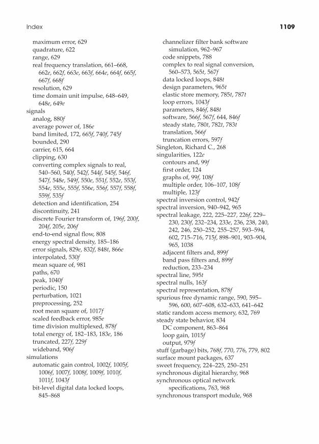
Index� 1109
maximum error, 629quadrature, 622range, 629real frequency translation, 661– 668,
662e, 662f, 663e, 663f, 664e, 664f, 665f, 667f, 668f
resolution, 629time domain unit impulse, 648– 649,
648e, 649esignals
analog, 880faverage power of, 186eband limited, 172, 665f, 740f, 745fbounded, 290carrier, 615, 664clipping, 630converting complex signals to real,
540– 560, 540f, 542f, 544f, 545f, 546f, 547f, 548e, 549f, 550e, 551f, 552e, 553f, 554e, 555e, 555f, 556e, 556f, 557f, 558f, 559f, 535f
detection and identification, 254discontinuity, 241discrete Fourier transform of, 196f, 200f,
204f, 205e, 206fend- to- end signal flow, 808energy spectral density, 185– 186error signals, 829e, 832f, 848t, 866einterpolated, 530fmean square of, 981paths, 670peak, 1040fperiodic, 150perturbation, 1021preprocessing, 252root mean square of, 1017fscaled feedback error, 985etime division multiplexed, 878ftotal energy of, 182– 183, 183e, 186truncated, 227f, 229fwideband, 906f
simulationsautomatic gain control, 1002f, 1005f,
1006f, 1007f, 1008f, 1009f, 1010f, 1011f, 1043f
bit- level digital data locked loops, 845– 868
channelizer filter bank software simulation, 962– 967
code snippets, 788complex to real signal conversion,
560– 573, 565t, 567fdata locked loops, 848tdesign parameters, 965telastic store memory, 785t, 787tloop errors, 1043fparameters, 846f, 848tsoftware, 566f, 567f, 644, 846fsteady state, 780t, 782t, 783ttranslation, 566ftruncation errors, 597f
Singleton, Richard C., 268singularities, 122e
contours and, 99ffirst order, 124graphs of, 99f, 108fmultiple order, 106– 107, 108fmultiple, 123f
spectral inversion control, 942fspectral inversion, 940– 942, 965spectral leakage, 222, 225– 227, 226f, 229–
230, 230f, 232– 234, 233e, 236, 238, 240, 242, 246, 250– 252, 255– 257, 593– 594, 602, 715– 716, 715f, 898– 901, 903– 904, 965, 1038
adjacent filters and, 899fband pass filters and, 899freduction, 233– 234
spectral line, 595tspectral nulls, 163fspectral representation, 878fspurious free dynamic range, 590, 595–
596, 600, 607– 608, 632– 633, 641– 642static random access memory, 632, 769steady state behavior, 834
DC component, 863– 864loop gain, 1015foutput, 979f
stuff (garbage) bits, 768f, 770, 776, 779, 802surface mount packages, 637sweet frequency, 224– 225, 250– 251synchronous digital hierarchy, 968synchronous optical network
specifications, 763, 968synchronous transport module, 968
1110� Index
T
Taylor series expansion, 120temperature, 614– 615, 618, 621– 622, 636–
637, 761, 772, 834– 844, 869, 995, 1004operational, 618voltage controlled crystal oscillators,
637time division multiplex processing, 680,
878f, 880f, 957, 967– 969, 973frequency division multiplex
conversion, 873– 881, 878f, 880ftransient response, 1014– 1015
automatic gain control circuits, 1030t, 1033f
data locked loops, 838e, 839e, 866texponential, 1019f, 1030tloop error, 1019fmeasuring, 1033frise time and, 866t
transition bands, 394f, 404f, 412f, 418f, 429ftranslate- and- filter operation, 917translation, 646, 875f
band limited signals, 665f, 676f, 731f, 740f, 745f
block diagram of, 746f, 748fcomplex signal, 746f, 747f, 748f, 750f,
751fdiscrete Fourier transform summation
filters, 893f, 894fnarrow band signals, 733f, 735fquarter band, 543, 553– 555, 553f, 554e,
556f, 558f, 568freal signal, 728f, 732f, 735f, 736f,
741f, 662fspectral magnitude, 733f
Treichler, John, 873Tukey, James W., 267two’s complement format, 585, 960f
U
underflow conditions, 769– 770, 772, 774, 777, 779
undersampling, 7, 193– 194, 536undershoot, 996– 997, 1018, 1020f, 1022funit circle, 2– 6, 3f, 4e, 9– 10, 12– 13, 38f, 39f,
77, 111– 112, 189– 190, 190e, 200, 201,
275– 276, 279– 282, 285, 286f, 290, 291f, 296, 297f, 318, 322– 323, 336, 338– 340, 342, 350, 352, 355, 359– 361, 365– 366, 365f, 373f, 373, 377, 379, 373, 377, 379, 473– 474, 479, 493, 495, 522, 526, 690– 691, 694, 696– 697, 704, 708– 709, 888– 889, 889f, 915, 917– 918, 934, 937
unit delay, 292f, 293e, 294e, 295funity coefficients, 491up sampling, 436, 450f
V
vector multiplication, 189VHSIC hardware description language,
543, 792Visual C/C++, 395voltage controlled crystal oscillator, 637,
807, 821– 826, 828– 835, 840– 842, 845, 847– 851, 866– 871
control voltage, 824tdesign example, 832edigital error signals and, 832e, 866eerror response versus voltage, 831efrequency, 821f, 830f, 832ffrequency response, 866efrequency response versus voltage,
830f, 831e, 866eideal frequency, 832finput error voltage, 849flinear, 830fnonlinearity, 822operating region, 831output frequency, 824t, 830fsynthesized frequency, 849f
voltageanalog output, 820tcurve, 832ferror, 849f, 819f, 821f, 849ffractional output, 824tmultiplying D/A converter reference
pin, 822reference, 818– 823, 819f, 821f, 830,
845, 869voltage controlled crystal oscillator
control voltage, 824t
Index� 1111
voltage controlled crystal oscillator frequency versus, 830f, 831e, 832f, 866e
Von Hann, Julius, 243
W
waveformscosine waves, 3, 6, 8, 11, 131, 148, 174,
182, 190, 200, 205, 225, 227, 657, 662, 703– 704, 711– 716, 728, 950– 952, 955f
discrete, 213f, 217fduty cycle pulsed, 141t, 143f, 144teven symmetric triangular, 144f, 149ffrequency spectrum of, 161e, 162fgraphs of, 160finfinite length, 158mapped, 11fnegative exponential, 748noise and, 257fnormalizing, 149e, 150epulse, 160f, 161e, 162f, 213f, 217fpurity of, 592sawtooth, 577f, 578sinusoidal, 2– 12, 11f, 131, 175, 205, 227,
235, 240, 257f, 258, 576, 581, 582– 585, 589– 590, 599, 604, 626, 629, 641, 704, 708– 716, 801, 1011– 1012, 1038
spectrum, 217fsquare, 137f, 140, 154, 157– 158, 596– 600,
597f, 598e, 598f, 599e, 602, 614, 801, 821
triangle, 142– 143, 147, 148t, 154– 155, 157voltage, 130
weighting function, 394, 396ewiper arms, 443, 445, 453– 456, 455f, 460,
462, 549– 552, 555, 557– 558, 906f, 907, 912
write pointers, 793f, 811, 812f, 813f, 816f, 819f, 821f
Z
zerosaliased, 521fcomplex, 344e, 344f, 345e, 345f, 347f, 375fcritical, 388ecrossings along the spectrum, 163
inserted, 458f, 545finterleaved sequences, 546magnitude tabulations for, 370tpole- zero, 373freal, 335f, 337e
z- transform, xvii, 271– 382applications of, 350– 380common pairs, 304– 308, 304e, 305t,
306e, 306t, 308econvergence of, 279– 289, 281f, 282f,
283e, 284e, 285e, 286e, 286f, 287e, 288e, 288f, 289f
convolution of sequences, 301– 303, 302e, 303e
differentiation and, 299, 299eequations using, 334– 350equations using, 380– 381evaluating, 275ffinal value theorem, 300– 301, 300eFourier transform and, 274efrequency response, 276einitial value theorem, 300– 301, 300einverse, 308– 334, 308e, 309e, 310e, 311e,
311f, 312e, 313e, 329e, 330eleft- sided, 277– 278, 277e, 281f, 286e,
287e, 288flinearity, 297mechanics of, 274– 277modifying an existing circuit, 363– 380multiplication of sequences, 303– 304, 304eone- sided, 380epartial fraction expansion method,
312– 328, 312e, 313epower series expansion method,
308– 311, 308e, 309e, 310e, 311e, 311fproperties of, 292– 304recursive accumulator, 350– 363residue method, 328– 334, 329e, 330eright- sided, 278, 278e, 281f, 284e, 285e,
286f, 298– 299, 298e, 300– 301, 300e, 380e
shifting, 297– 298, 298e, 380esimplifying signal processing with, 275esystem stability and, 290– 292time sequences and, 274etwo- sided, 278– 279, 278e, 288e, 289f, 380eunit delay, 292– 297