practical considerations in the design of experiments for

6/21/2019

1

Practical Considerations in the Design of Experiments for

Binary Data

Practical DOE for Binary Data

Martin Bezener

Stat-Ease, Inc.

1. Introduction

2. Some Simple Examples

3. Practical Tips and Tricks

4. Conclusion

Practical DOE for Binary Data 2

6/21/2019

2

1. Introduction2. Some Simple Examples


4. Conclusion


• Choose factors and define the design space

• Determine the appropriate experimental design

• Perform the experiment

• Analyze data and check for problems

• If the response continuous, usually use Ordinary Least Squares, possibly with a transform

• Optimize

• Follow up experiments needed?

• Confirm

• Fix problems resulting from confirmation?

• Finish

Introduction

A Typical Experimentation Sequence:

The DOE Process


6/21/2019

3

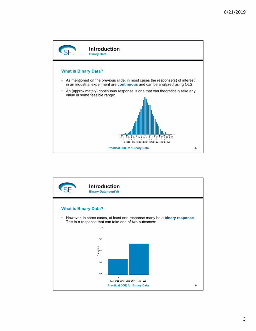
• As mentioned on the previous slide, in most cases the response(s) of interest in an industrial experiment are continuous and can be analyzed using OLS.

• An (approximately) continuous response is one that can theoretically take any value in some feasible range:

Introduction

What is Binary Data?

Binary Data


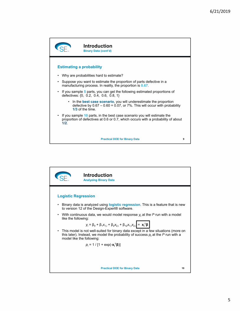
• However, in some cases, at least one response many be a binary response. This is a response that can take one of two outcomes:

Introduction

What is Binary Data?

Binary Data (cont’d)


6/21/2019

4

• Some common examples of binary responses:

• Quality Engineering: {Pass, Fail}

• Pharma: {Survived, Didn’t Survive}

• Medical: {Disease Present, Disease Absent}

• Marketing: {Clicked on Ad, Didn’t Click on Ad}

• Food: {Dough Rises, Dough Doesn’t Rise}

• …

• Experiments may include both continuous and binary responses.

• A binary response is often considered a categorical response.

Introduction

Some Examples



• A primary use of binary data is to estimate a probability

• Binary data is less informative than continuous data.

• Cohen (1983) shows that “discretizing” continuous data is equivalent to throwing away 40-60% of the observations.

TIP: Designs that have a binary response will generally require many more runs compared to an equivalent design with a continuous response.

TIP: If you have continuous data, analyze it as continuous data. If you need to choose a threshold on which to make a binary decision, do so after the data analysis, not before.

Introduction

Some Interesting Features of Binary Data:



6/21/2019

5

• Why are probabilities hard to estimate?

• Suppose you want to estimate the proportion of parts defective in a manufacturing process. In reality, the proportion is 0.67.

• If you sample 5 parts, you can get the following estimated proportions of defectives: {0, 0.2, 0.4, 0.6, 0.8, 1}

• In the best case scenario, you will underestimate the proportion defective by 0.67 – 0.60 = 0.07, or 7%. This will occur with probability 1/3 of the time.

• If you sample 10 parts, in the best case scenario you will estimate the proportion of defectives at 0.6 or 0.7, which occurs with a probability of about 1/2.

Introduction

Estimating a probability



• Binary data is analyzed using logistic regression. This is a feature that is new to version 12 of the Design-Expert® software.

• With continuous data, we would model response yi at the ith run with a model like the following:

yi = β0 + β1x1,i + β2x2,i + β12x1,ix2,i = xiTβ

• This model is not well-suited for binary data except in a few situations (more on this later). Instead, we model the probability of success pi at the ith run with a model like the following:

pi = 1 / [1 + exp(-xiTβ)]

Introduction

Logistic Regression

Analyzing Binary Data


6/21/2019

6

Introduction

One Factor Illustration

Analyzing Binary Data (cont’d)


• Consider the following data:

Factor Reps # Success0 9 01 8 12 12 33 15 144 12 12

• A linear logistic model can befit to this data (right).

Introduction

How about OLS?

Analyzing Binary Data (cont’d)


6/21/2019

7

IntroductionAnalyzing Binary Data (cont’d)


• Both OLS and logistic regression give reasonably close predictions of probabilities between 0.2 and 0.8 (approximately).

• Logistic regression, however, will give reasonable predictions of probabilities between 0 and 1.

• Even if OLS and logistic regression models give reasonably close predictions, the standard errors (and hence inference) may be very different.

TIP: Use logistic regression to analyze binary data. Don’t try to force an OLS model to 0/1 data.

Introduction

A Comparison of Two Tools:

OLS vs Logistic Regression


6/21/2019

8

• Multinomial response

• A multinomial response is a categorical response. Similar to binary, but can take more than two values.

• Modelled using Multinomial Logit Models

• Example: Discrete Choice Experiments

• Count response

• A non-negative integer response: {0, 1, 2, 3, 4, 5, …}

• Modelled using Poisson Regression (coming in v13)

• Example: Number of defects on a metal sheet

Introduction

Other Types of Responses You May Encounter:

Other Types of Responses


1. Introduction

2. Some Simple Examples3. Practical Tips and Tricks

4. Conclusion


6/21/2019

9

• Our first example involves only one factor, but easily illustrates a number of interesting features of binary data

• An aircraft fastener manufacturer wanted to study the ability of a new fastenerto withstand different loads

• Only one factor was varied: Load from 2500 psi to 4300 psi

• A number of fasteners were tested at 10 different loads in the factor range

• The goal was to see how Load affected the probability of a fastener failing.

Some Simple Examples

One Factor Example

Fastener Example


• The following experimental design was used. No information was provided to justify the choice of this design.

Force # Replicates2500 502700 702900 1003100 603300 403500 853700 903900 504100 804300 65 Total = 690


The Design

Fastener Example


6/21/2019

10

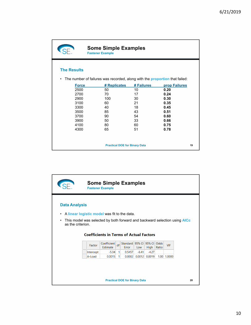
• The number of failures was recorded, along with the proportion that failed:

Force # Replicates # Failures prop Failures2500 50 10 0.202700 70 17 0.242900 100 30 0.303100 60 21 0.353300 40 18 0.453500 85 43 0.513700 90 54 0.603900 50 33 0.664100 80 60 0.754300 65 51 0.78


The Results

Fastener Example


• A linear logistic model was fit to the data.

• This model was selected by both forward and backward selection using AICcas the criterion.


Data Analysis

Fastener Example


6/21/2019

11

Some Simple ExamplesFastener Example


• The process of separating mixtures of compounds is called chromatography. Ultra high performance liquor chromatography (UHPLC) is the gold standard for commercially available chromatograph techniques, but it uses very expensive equipment to provide the ultra high pressure.

• A research team tries to create a polymeric column that will have a pore size and skeleton thickness to achieve the same efficiency as UHPLC techniques but with lower pressure and hence lower cost.


A Mixture Experiment with a Binary Response

Column Example


6/21/2019

12

• A formulation does not always create a polymer that is completely solid, which is called a “homogeneous” column.

• The pores are not always interconnected, meaning the compound will not flow through the column.

• Immediate Goal: Design an experiment to model how the blending properties of water, monomer, and surfactant affect the probability of creating an acceptable column (one that is homogeneous and capable of flowing through the column).


Problem

Column Example


Component Lower Bound Upper Bound

A: Water 70 80

B: Monomer 10 25

C: Surfactant 2 8

D: Initiator 0.02 0.025

E: Salt 0.8 0.8

Total = 100 weight %

Also, we need 0.002 < D/B < 0.01


Mixture Components, Ranges, and Constraints

Column Example


6/21/2019

13

• The design was built using Design-Expert version 12.

• Two binary responses were measured for each formulation:


The Design

Column Example


Name Units

homogeneous 0‐No 1‐Yes

flow 0‐No 1‐Yes


Homogeneous Results…

Column Example


6/21/2019

14


Flow Results…

Column Example



Joint Optimization

Column Example


6/21/2019

15

• The joint maximum probability for both responses occurs at:

• Notice that two of the components (B and C) are at their maximums.

• TIP: Consider expanding the ranges of B and C a bit in a follow-up experiment.


Joint Optimization

Column Example



Check Confidence Intervals

Column Example


• The lower bound on the confidence interval for flow is 0.48 (less than half!).

• TIP: Consider doing additional follow up runs in a region around this optimum to improve precision.

6/21/2019

16

1. Introduction


3. Practical Tips and Tricks4. Conclusion


• TIP 1: Designs that have a binary response will generally require many more runs compared to an equivalent design with a continuous response.

• TIP 2: If you have continuous data, analyze it as continuous data. If you need to choose a threshold on which to make a binary decision, do so after the data analysis, not before.

• TIP 3: Use logistic regression to analyze binary data. Don’t try to force an OLS model to 0/1 data.

• Now we’ll go through two relevant practical issues:

• building designs for binary data

• confirmation

Practical Tips and Tricks

Some of the things we’ve discussed so far:

Recap of Previously Mentioned Tips


6/21/2019

17

• Building designs for binary data is generally harder than building designs for continuous data.

• This is due to the (previously mentioned) fact that binary data is less informative than continuous data.

• The canned designs for continuous data, such as Central Composite RSMs, or Simplex Lattice Mixture designs, will be too small for a binary responses.

• Optimal designs are also more tricky. Unlike designs for a continuous response, optimal designs for binary data depend on the actual values of the regression coefficients, which of course, are unknown.

• The construction of optimal experimental designs for binary data is still an active research area.

Building Designs for Binary Data

The Issues

Issues


• A D-optimal design for a continuous response and linear model minimizes the determinant of the variance-covariance matrix of the regression coefficients:

D(X) = | σ2(XTX)-1 |

where X is the n x p model matrix.

• Because of the constant variance assumption under linear model, the σ2 is constant and we simplify this to

D(X) = | (XTX)-1 |

• Notice that the D-optimal design X does not depend on σ2 or the regression coefficients. This design will be D-optimal for all sets of regression parameters.

• An I-optimal design would suffer from these same issues.


D-Optimal Designs

Issues


6/21/2019

18

• A D-optimal design for a binary response and logistic model minimizes the determinant of the variance-covariance matrix of the regression coefficients:

D(X) = | (XTWX)-1 |

where W is a matrix that depends on the regression parameters β.

• Example (Chipman & Welch, 1996): Suppose we have two factors of interest and a binary response. We are interested in fitting a linear logistic model.

1 / [1 + exp(-u)] where u = β0 + β1x1 + β2x2

• Four 12-run designs are generated for the following combinations of (β1, β2): (1, 1) (1, 3) (3, 1) (3, 3)


D-Optimal Designs

Issues


Building Designs for Binary DataResults


6/21/2019

19

• Having some idea of what the regression coefficients are beforehand will make building an experiment for binary data much easier.

• Bayesian methods have been developed that reduce the dependence of design optimality on the regression coefficients.

• Space-filling points are very useful.

• Sequential experimentation is key!

• Pilot study to obtain rough estimate of coefficients

• Re-define space based on the results of pilot study

• Optimize, check confidence intervals widths, add runs if necessary

• Continue until satisfied


Practical Guidelines

Strategies


• After finding an optimum, it’s ideal to do a few (?) follow-up runs to validate the results.

• Prediction intervals would typically be used with continuous responses to validate an optimum.

• What’s a prediction interval when there are only two possible responses (0/1)?

• An alternative strategy must be used for binary data.

• In general, confirmation is much more difficult with binary data and is likely only useful to catch extreme problems with the model.

Confirmation with Binary DOE

What is confirmation?

What’s the Story?


6/21/2019

20

• Let’s revisit the column example.

• We got the following results at the optimal blend for homogeneous:

Response prediction low CI upper CIhomogeneous 0.97 (0.75, 0.99)

• Suppose we do 10 confirmation runs (columns). We can treat the predicted probability as fixed values and do a simple z-test for proportions.

• Obviously, there is no realistic way to check if p is actually higher than 0.97 because you’ll almost always get 10 homogenous columns of out 10 trials.

• But if p is actually 0.97, the probability we’ll see fewer than 9 homogeneous columns in 10 trials is 0.035 (3.5%).

• So a rule of thumb would be that 8 or fewer homogenous columns out of 10 trials indicates a potential problem at the 5% false alarm rate.


Simple Strategy

What to Do?


• This is an extremely coarse check!

• If the true p is 0.80 (instead of the estimated 0.97), the confirmation will only detect a problem with probability 0.6 (60%).

• But 0.8 vs 0.97 is a huge difference!

• The moral of the story is that this is a good strategy for detecting very serious issues, but many minor issues will be missed unless you have a very large confirmation sample, likely too large to be feasible.


Simple Strategy

What to Do?


6/21/2019

21

• The simple strategy assumes the predicted proportion is fixed and free of error. Of course, this is not true, as it’s only an estimate based on our model.

• The simple strategy is probably too liberal, meaning it will detect problems more often than we’d like.

• Proposed Solution: Use the simple strategy, but apply it to the lower limit of the confidence interval.

Response prediction low CI upper CIhomogeneous 0.97 (0.75, 0.99)

• Remember the confidence interval of (0.75, 0.99) gives us a range of plausible p that we can expect to see in the long run, which means it’s not impossible that we observe only 75% homogeneous columns at the optimal formulation.


Advanced Strategy

A Better Approach


• So we can apply the Simple Strategy discussed before to the lower bound of 0.75.

• With 10 confirmation runs, it’s impossible to detect a higher alternative at a 5% false alarms rate, since you’ll see 10 out of 10 homogenous columns with probability 0.056 (5.6%).

• With 10 confirmation runs, a cutoff at the 5% false alarm rate would be 4 or fewer homogenous columns.

• This is a far more conservative cutoff vs. the previous cutoff of 8. Chances are the “best” cutoff for detecting issues lies in the set {4, 5, 6, 7, 8} – somewhere in between the two.


Advanced Strategy

A Better Approach?


6/21/2019

22

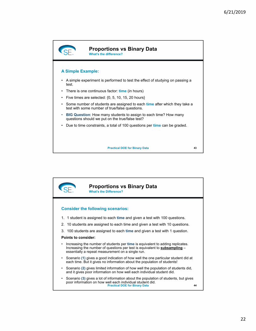
• A simple experiment is performed to test the effect of studying on passing a test.

• There is one continuous factor: time (in hours)

• Five times are selected: {0, 5, 10, 15, 20 hours}

• Some number of students are assigned to each time after which they take a test with some number of true/false questions.

• BIG Question: How many students to assign to each time? How many questions should we put on the true/false test?

• Due to time constraints, a total of 100 questions per time can be graded.

Proportions vs Binary Data

A Simple Example:

What’s the difference?


1. 1 student is assigned to each time and given a test with 100 questions.

2. 10 students are assigned to each time and given a test with 10 questions.

3. 100 students are assigned to each time and given a test with 1 question.

Points to consider:

• Increasing the number of students per time is equivalent to adding replicates. Increasing the number of questions per test is equivalent to subsampling –essentially a repeat measurement on a single run.

• Scenario (1) gives a good indication of how well the one particular student did at each time. But it gives no information about the population of students!

• Scenario (2) gives limited information of how well the population of students did, and it gives poor information on how well each individual student did.

• Scenario (3) gives a lot of information about the population of students, but gives poor information on how well each individual student did.


Consider the following scenarios:

What’s the Difference?


6/21/2019

23

1. 1 student is assigned to each time and given a test with 100 questions.

2. 10 students are assigned to each time and given a test with 10 questions.

3. 100 students are assigned to each time and given a test with 1 question.

More Points to Consider:

• Scenario (1) and (2) can be analyzed with OLS, possibly with the arcsine sqrt transform, or with a mixed effects logistic regression model (not yet implemented).

• Scenario (3) can be analyzed with logistic regression (new in version 12).

• But… which is better? Or is there a compromise in between these scenarios that works best?


Consider the following scenarios:



• Some simulation work would need to be done, but intuitively it seems that scenario (3) should work best, in general.

• If there is very little student-to-student variability, then perhaps (2) may be an acceptable option.

• This question arises all the time in my experience in manufacturing applications: do I make a few large batches at each run, or do I make many batches that are smaller, possibly of size one?


The Answer:



6/21/2019

24

1. Introduction



4. Conclusion


• Binary data is usually analyzed using logistic regression. Don’t try to force familiar methods to binary data – take some time to learn the proper tools! Design-Expert 12 makes this easy to do.

• Don’t turn continuous data into binary data before analyzing your model. If you make your data binary, do so after analyzing the continuous response.

• Choosing a design is tricky – start small and iterate until you achieve your desired results. You may need to tweak component ranges and add more runs.

• Confirmation is more limited with binary data.

Conclusion

Take Home Points

Wrap Up


6/21/2019

25

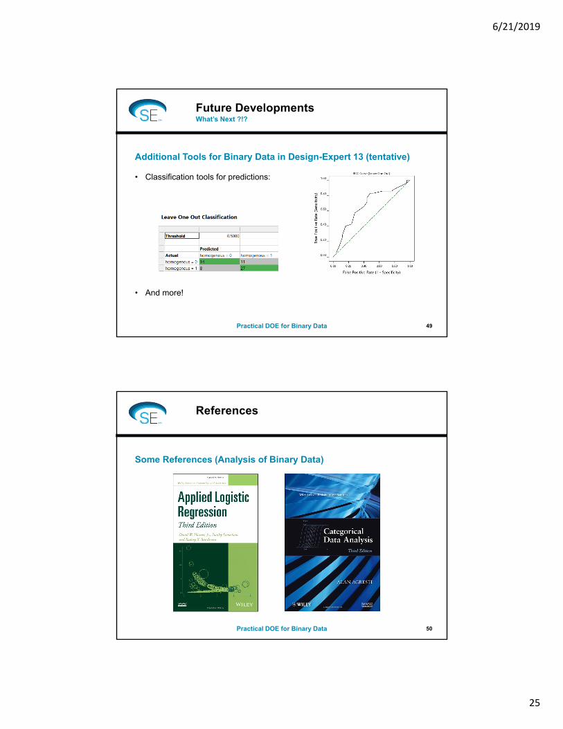
• Classification tools for predictions:

• And more!

Future Developments

Additional Tools for Binary Data in Design-Expert 13 (tentative)

What’s Next ?!?


References

Some References (Analysis of Binary Data)


6/21/2019

26

References

Some References (Design Experiments for Binary Data)


?

??

??

?

?

Martin Bezener

practical considerations in the design of experiments for

Documents