A

Aiigo5©

K

1

otpimsococsprv

t[

0d

Available online at www.sciencedirect.com

Precision Engineering 32 (2008) 309–318

Practical control method for ultra-precision positioningusing a ballscrew mechanism

Guilherme Jorge Maeda, Kaiji Sato ∗Interdisciplinary Graduate School of Science and Engineering, Tokyo Institute of Technology, 4259 Nagatsuta, Midori-ku, Yokohama 226-8502, Japan

Received 7 March 2007; received in revised form 18 September 2007; accepted 26 October 2007Available online 24 November 2007

bstract

This paper describes a practical control method for nanometer level point-to-point positioning (PTP) using a conventional ballscrew mechanism.nominal characteristic trajectory following controller (NCTF controller) is used for the ultra-precision positioning. The controller design, which

s comprised of a nominal characteristic trajectory (NCT) and a PI compensator, is free from exact modeling and parameter identification. The NCTs determined from an open-loop experiment and the PI compensator is used to make the mechanism motion to follow the NCT. The compensator

ain values are restricted by the practical stability limit of the control system, which is easy to determine. Using a high integral gain causes excessivevershoot, so an antiwindup integrator is used to improve the system performance. The NCTF control system achieves a positioning resolution ofnm and is robust against friction variations.2007 Elsevier Inc. All rights reserved.

on; Ba

pmeattdmdtbc

antt

eywords: Nanopositioning; Ultra-precision positioning; Point-to-point; Fricti

. Introduction

Precision positioning systems that can achieve an accuracyn the order of micrometers or nanometers are essential inhe optical, semiconductor, and nanotechnology industry. Theseositioning systems usually have one or more elements thatntroduce friction, like motors with brushes and/or bearings with

echanical contact. Friction is well known to cause steady-tate and tracking errors, to limit cycles and to slow the motionf the mechanism. Thus, it is important to consider frictionompensation in controller design. However, controller designf mechanisms with friction tends to be difficult because: (1)haracteristics of mechanisms with friction are nonlinear, thusimple controllers like PID controllers do not offer the bestossible performance and (2) friction compensation usuallyequires the identification of friction characteristics, which canary.

In order to compensate for friction, efforts have been madeo understand the effects of friction on control performance1] and its dynamics [2,3]. Control systems for precision/ultra-

∗ Corresponding author. Tel.: +81 45 924 5045; fax: +81 45 924 5483.E-mail address: kaiji@pms.titech.ac.jp (K. Sato).

heu

ftt

141-6359/$ – see front matter © 2007 Elsevier Inc. All rights reserved.oi:10.1016/j.precisioneng.2007.10.002

llscrew; Antiwindup

recision positioning must compensate for friction on theicro-scale, which requires an understanding of the nonlin-

ar behavior of the mechanism before the breakaway torque ischieved [4–6]. Nevertheless, friction parameters, especially inhe microdynamic regime, tend to change with time and posi-ion [7,8] and seem to behave stochastically [5], making themifficult to predict exactly. Also, a complete model for macro-icrodynamics has to address the transition between the two

ynamics [9]. The inclusion of the friction dynamics as part ofhe control law does improve precision positioning [8,10–12],ut the controller design becomes time consuming and diffi-ult.

In this research, a conventional ballscrew mechanism is useds the friction mechanism. Although some studies have achievedanometric accuracy with a ballscrew system (e.g. [11–14]),his research differs significantly in the ease of design and con-rol structure. The controller used, called the NCTF controlleras a simple structure and its design method does not requirexact parameter identification, which makes it easy to design,nderstand, and adjust.

The NCTF control system has previously been used for dif-erent mechanisms, then evaluated and compared with otherypes of practical controllers. The influence of the NCTF con-roller parameters and actuator saturation were discussed for a

310 G.J. Maeda, K. Sato / Precision Engineering 32 (2008) 309–318

rbfdptatSNmbba

tpctcTt

iiatatSmti

2

wdn

tb

oTsvhutrv

fi(0its feedback position is determined by a laser position sensorwith resolution of 1.24 nm (Agilent: 10897B). The lead of theballscrew is 2 mm/rev and the maximum travel range of the tableis 55 mm.

Table 1Model parameters

Symbol Description Value

Km Torque constant of the motor 0.172 Nm/AM Table mass 3.57 kgJ Moment of inertia of the rotary parts 1.81 × 10−4 kg m2

Tfric Nonlinear friction –Tapp Applied torque to the ballscrew –Tfmax Coulomb friction 0.046 Nma

Fig. 1. Ballscrew mechanism used in this research.

otary mechanism in [15]. In [16,17], performance improvementy means of an antiwindup integrator was presented. The per-ormance of the NCTF controller was then compared to thoseelivered by conventional PID’s [15,18]. The NCTF controllererformance was also compared to two other practical con-rollers that address friction compensation: a PD controller withnonlinear proportional feedback compensator, and a PD con-

roller with a smooth nonlinear feedback compensator [19,20].ato et al. [21] designed and compared the performance of theCTF controller with that of a PID controller using a linearotor mechanism. In this study, the mechanism was driven

y a voice coil motor and had an adjustable-preload linearall guide. A positioning accuracy of better than 50 nm waschieved.

The purpose of this research is to clarify the NCTF con-rol method for a ballscrew mechanism used in ultra-precisionositioning. Mechanically, the ballscrew mechanism is moreomplex than the rotary and the linear motor mechanism men-ioned above. Regardless of the mechanical complexity, theontrol design method should still be easy and straightforward.he positioning accuracy and resolution are expected to be better

han 10 nm.This paper is organized as follows. The experimental setup is

ntroduced in Section 2. In Section 3, the NCTF controller designs explained, including the derivation of the design parametersnd analyses of the linear and the practical stability limit. Sec-ion 4 details the performance improvement by means of anntiwindup integrator. In Section 5, the performance of the con-rol system is evaluated by experiment and simulation. Finally,ection 6 discusses the feasibility of NCTF controller designethod for mechanisms with a large range of friction varia-

ion (including a pure inertia mechanism) and different NCTnclinations.

. Experimental setup

Fig. 1 shows a picture of the ballscrew mechanism,hich is the controlled mechanism in this study and Fig. 2etails the structure and dynamic model of the mecha-

ism.

The mechanism has several sources of friction: the dc motor,he preloaded double-nut, the linear ball guides, and the ballearings supporting the screw shaft. The overall combination

CKC

Fig. 2. Structure and dynamic model of the mechanism.

f nonlinear friction effects are modeled as the frictional torquefric in Fig. 2(b). The stiffness of the connection between thecrew and nut is represented as the spring constant Kn. Theibration between the screw and nut is damped by a damperaving coefficient Cn. Table 1 shows the description and val-es of the model parameters. Values of Tfmax and Csd tendo vary and depend on the warm-up condition. The simulatedesponses in Figs. 13 and 14 are calculated using their adjustedalues.

As additional information of interest, the PWM power ampli-er (Copley: 4122Z) is limited at 45V/6 A and the dc motorYaskawa: UGTMEM-06LB40E) has a back EMF constant of.086 Vs/rad. The controller sampling frequency is 5 kHz and

sd Viscous friction 0.00097 Nms/rada

n Spring constant (screw/nut) 8.3 × 105 N/m

n Damping coefficient (screw/nut) 1700 Ns/m

a May vary according to the warm-up condition.

G.J. Maeda, K. Sato / Precision Engineering 32 (2008) 309–318 311

3d

3

c(saumpfctat

attPtm

ietimiPedpift

3

dc

(

o

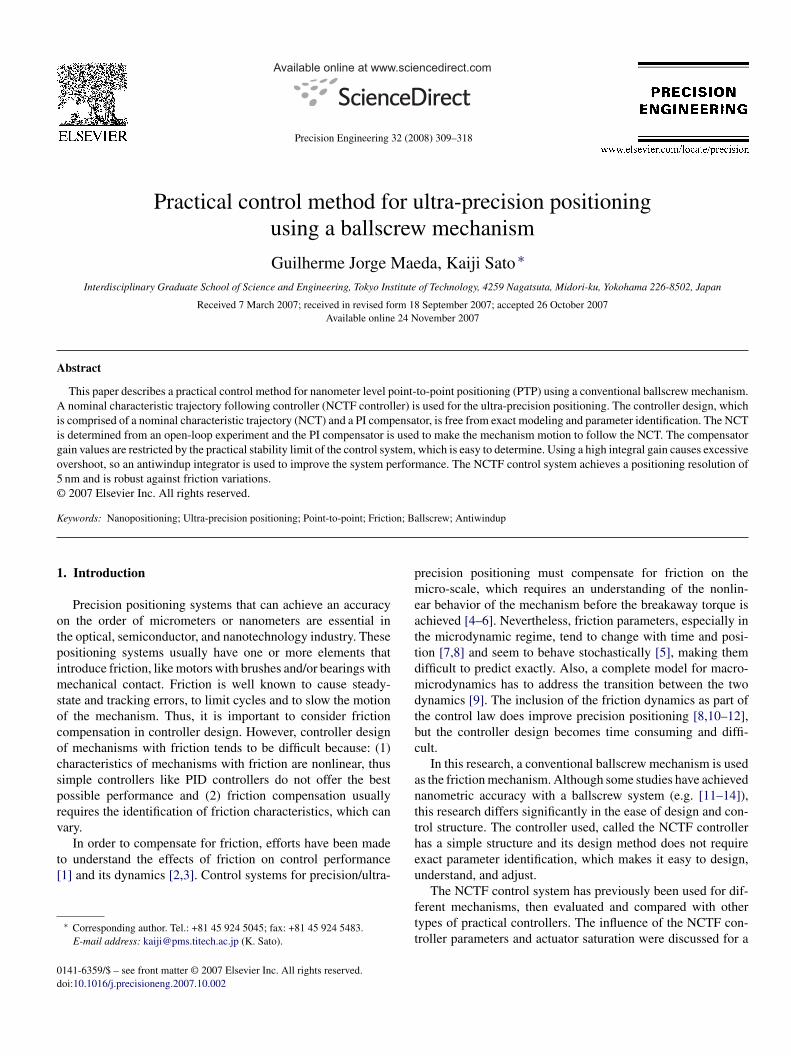
Fig. 3. Structure of the NCTF control system.

. NCTF control concept and its previous controlleresign for mechanisms with friction

.1. Concept

Fig. 3 shows the structure of the NCTF control system. Theontroller is composed of a nominal characteristic trajectoryNCT) and a PI compensator. The objective of the PI compen-ator is to make the mechanism motion follow the NCT, finishingt the origin of the phase-plane. The output of the NCT is a signalp, which is the difference between the actual error rate of theechanism (−x) and the error rate of the NCT. On the phase-

lane, the table motion is divided into a reaching phase and aollowing phase. During the reaching phase, the compensatorontrols the table motion to achieve the NCT. The next step ishe following phase, where the PI compensator causes the mech-nism motion to follow the NCT, leading it back to the origin ofhe phase-plane.

The NCT is constructed from the actual response of the mech-nism influenced by the friction and saturation effects. Thushe PI compensator tuned necessarily has the ability to makehe mechanism motion follow the NCT macroscopically. TheI compensator works for reduction of the difference between

he NCT and the actual motion when disturbance forces andechanism characteristic changes increase the difference.In a large working range where the saturation characteristic

nfluences the mechanism motion, the reduction of the differ-nce between them is desired so that the mechanism reacheshe reference quickly without significant overshoot. Howevern a small working range, the elimination of static deviation is

ore important than the reduction of the difference. As shownn Fig. 4, the NCTF controller can be expressed using a variableI element and a PD element. The NCT works as a variable gainlement. The variable PI element has larger gain as the errorecreases. The gain maximizes near the origin on the phase-lane, that is, near the reference position. This characteristic

s useful to quickly eliminate the static deviation caused by theriction. The characteristic also tends to reduce the vibration andhe overshoot [21].

Fig. 4. Expression of the NCTF control system.

.2. Design procedure

The theoretical discussion and the previous NCTF controlesign method is detailed in [15,21]. The design of the NCTFontroller is comprised of three steps:

(i) The mechanism is driven with an open-loop stepinput while its displacement and velocity are measured.Fig. 5(a) shows the open-loop response of the ballscrewmechanism.

(ii) The NCT is constructed on the phase-plane using thedisplacement and velocity of the mechanism during thedeceleration. Fig. 5(b) shows the NCT constructed fromthe open-loop experiment. In this figure, the trajectory fromthe response includes a circling motion caused by a spring-like behavior. This circling motion has negative effects onpositioning and should be eliminated [21,22]. In order todo so, the NCT is linearized with a straight line close to theorigin.

iii) The PI compensator is designed using the open-loopresponse and the NCT information. The PI gains are chosenwithin the stable operation region which can be previouslycalculated independently of the actual mechanism charac-teristic.

The derivation of the NCTF controller parameters are basedn a linear macrodynamic model expressed as

X

U= K

α

s(s + α)(1)

312 G.J. Maeda, K. Sato / Precision Engineering 32 (2008) 309–318

Wt

x

Ntα

c

K

K

Wobioca

n[bhid

4p

4

sotwis

aectmg

ζ

Ebb

Fig. 5. Open-loop response and construction of the NCT.

hen the value of u is constant with amplitude ur, and zero afterr (see Fig. 4(a)), parameter K becomes

f = Kurtr → K = xf

urtr(2)

Fig. 6 shows the block diagram of the continuous closed-loopCTF control system with the simplified object model near

he NCT origin (where the NCT is linear and has an inclination= −m). The proportional and integral compensator gains are

alculated from

P = 2ζωn

αK(3a)

I = ω2n

αK(3b)

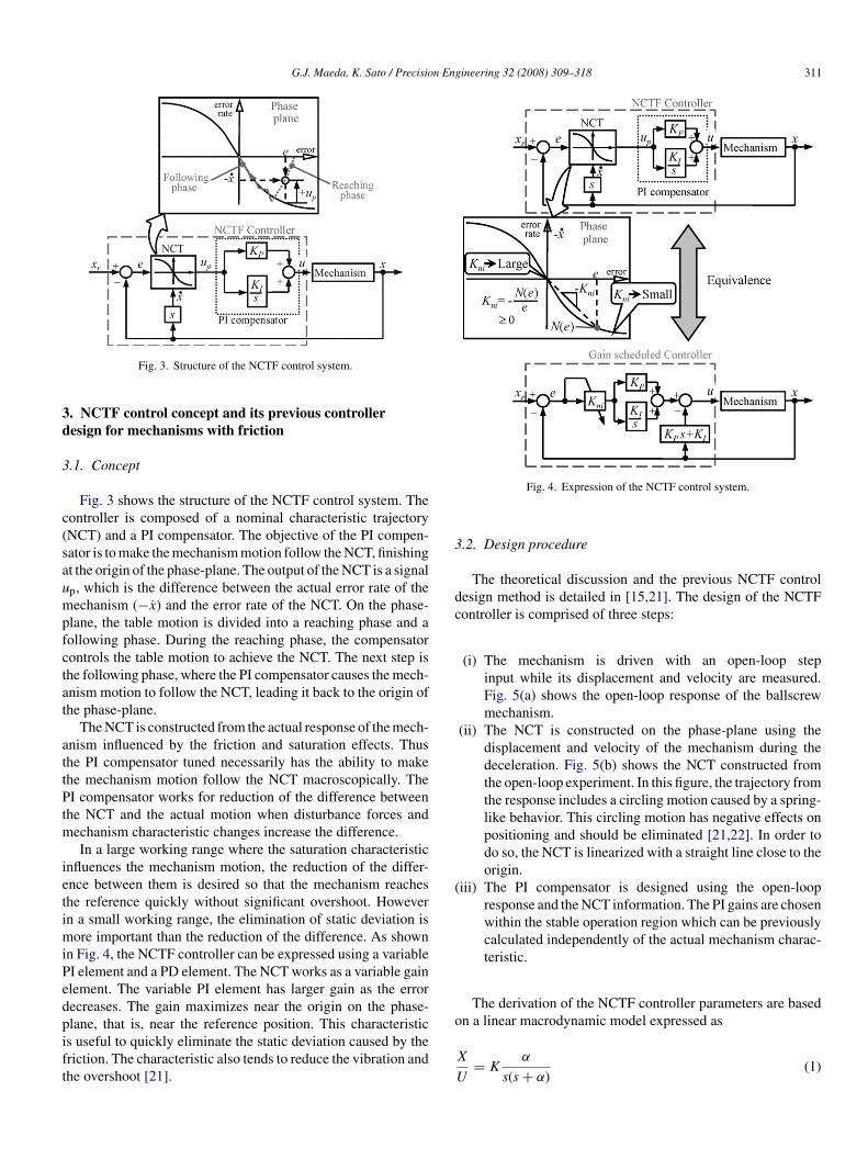
hen choosing ζ and ωn, the designer must consider the stabilityf the control system. Regarding the digital system, a linear sta-ility analysis is carried out with the sampled-data system shown

n Fig. 7 Applying the Jury’s test ([23], p. 35), a numerical plotf the stability limit is shown in Fig. 8. The linear stability limitan be calculated independently of the actual mechanism char-cteristic. The limit also has negligible variations on the αT axis.

Fig. 6. NCTF control system with the simplified object model.

ζ

tacpTctc

Fig. 7. Sampled-data system used for a linear stability analysis.

However the stability limit is too limited. Coulomb frictioneglected in Fig. 7 is known to increase the stability of the system1], allowing for the use of higher gains than those predictedy a linear analysis. The higher gains are expected to produceigher positioning performance. Thus the practical stability limits necessary for selecting the higher gains in step (iii) of theesign procedure.

. Practical stability limit and choice of the designarameters

.1. Decision of practical stability limit

This section introduces a simple method to find the practicaltability limit of the NCTF control system. From Fig. 8 it isbserved that the integral element has a negligible influence onhe stability of the linear system. For the following analysis, itill also be assumed that the integral element has a negligible

nfluence on the stability of the actual system. Experiments andimulations will show that this assumption is valid.

The practical stability limit is found by driving the mech-nism with the NCTF controller using only the proportionallement. The value of the proportional gain is increased untilontinuous oscillations are generated. The determined propor-ional gain is called KPu (2.4 As/mm in the case of the ballscrew

echanism), which represents the actual ultimate proportionalain. Using Eq. (3a), the practical stability limit ζprac is given as

prac = KPu

(αK

2ωn

)(4)

q. (4) represents the maximum values allowed for a given ζ,efore the control system becomes unstable. In the case of theallscrew mechanism, Eq. (4) becomes

prac = 2.4

(505 × 32.3

2ωn

)(5)

In order to prove the suitability of ζprac, the NCTF con-roller (using the proportional and integral elements), is designeds follows: for a fixed value of ωnTk (where k = 1, . . ., 7), theompensator gains are calculated from Eqs. (3a) and (3b). Thearameter ζk is increased until the system achieves instability.

he points defined by ζk and ωnTk are plotted in Fig. 9. The pro-edure performed both experimentally and by simulations usinghe mechanism model in Fig. 2(b). As the results show, ζprac fitslosely to all the points representing the NCTF control stability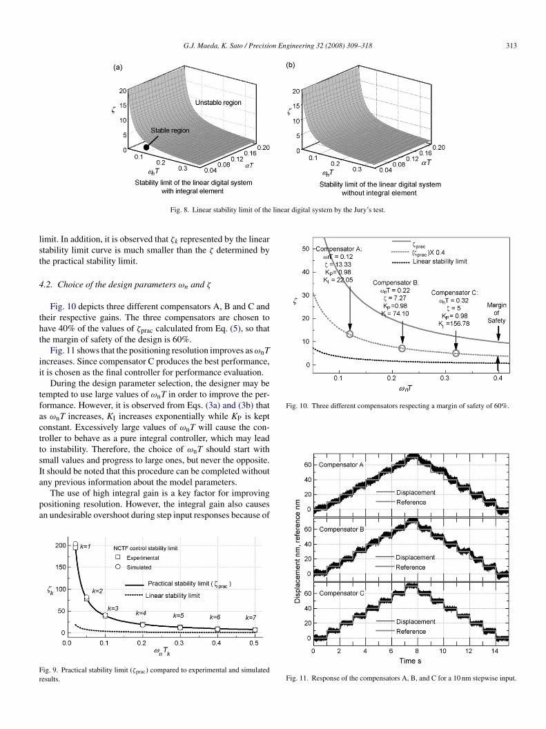

G.J. Maeda, K. Sato / Precision Engineering 32 (2008) 309–318 313

linear digital system by the Jury’s test.

lst

4

tht

ii

tfacttsIa

pa

Fr

Fig. 10. Three different compensators respecting a margin of safety of 60%.

Fig. 8. Linear stability limit of the

imit. In addition, it is observed that ζk represented by the lineartability limit curve is much smaller than the ζ determined byhe practical stability limit.

.2. Choice of the design parameters ωn and ζ

Fig. 10 depicts three different compensators A, B and C andheir respective gains. The three compensators are chosen toave 40% of the values of ζprac calculated from Eq. (5), so thathe margin of safety of the design is 60%.

Fig. 11 shows that the positioning resolution improves as ωnTncreases. Since compensator C produces the best performance,t is chosen as the final controller for performance evaluation.

During the design parameter selection, the designer may beempted to use large values of ωnT in order to improve the per-ormance. However, it is observed from Eqs. (3a) and (3b) thats ωnT increases, KI increases exponentially while KP is keptonstant. Excessively large values of ωnT will cause the con-roller to behave as a pure integral controller, which may leado instability. Therefore, the choice of ωnT should start withmall values and progress to large ones, but never the opposite.t should be noted that this procedure can be completed without

ny previous information about the model parameters.

The use of high integral gain is a key factor for improvingositioning resolution. However, the integral gain also causesn undesirable overshoot during step input responses because of

ig. 9. Practical stability limit (ζprac) compared to experimental and simulatedesults. Fig. 11. Response of the compensators A, B, and C for a 10 nm stepwise input.

314 G.J. Maeda, K. Sato / Precision Engineering 32 (2008) 309–318

F

tu

tttAppfs

tcf

�

wcv

aeFF

trsf

5

NTc

ig. 12. NCTF controller structure with the conditionally freeze antiwindup.

he integrator windup effect. Thus, antiwindup integrators areseful for performance improvement.

Up until now, antiwindup integrators with the NCTF con-roller have been applied to a rotary positioning system: aracking antiwindup [16] and a conditionally freeze integra-or [17]. Both methods were shown to improve robustness.lthough the tracking antiwindup method has only one designarameter, there are no clear rules on how to determine a properarameter value, except for rules of thumb. The conditionallyreeze integrator rule requires only a maximum control outputignal as a design parameter, which is easy to determine.

Due to the ease of implementation, this research employshe conditionally freeze integrator [17]. The antiwindup elementontrols the input of the integrator, as shown in Fig. 12, with theollowing rule:

ui ={

0, |uo + ui| > us and e · ui ≥ 0

e, otherwise(6)

here uo is the proportional control signal, ui is the integratedontrol signal,�ui is the change rate of ui, and us is the maximumalue of the control signal.

The maximum output control signal of the ballscrew mech-

nism, which defines the saturation of the actuator, is 6 A. Theffect of the antiwindup on positioning performance is shown inig. 13, where compensator C is used in the NCTF controller.or a step input of 20 mm, the overshoot was reduced from 9.3%

f

1l

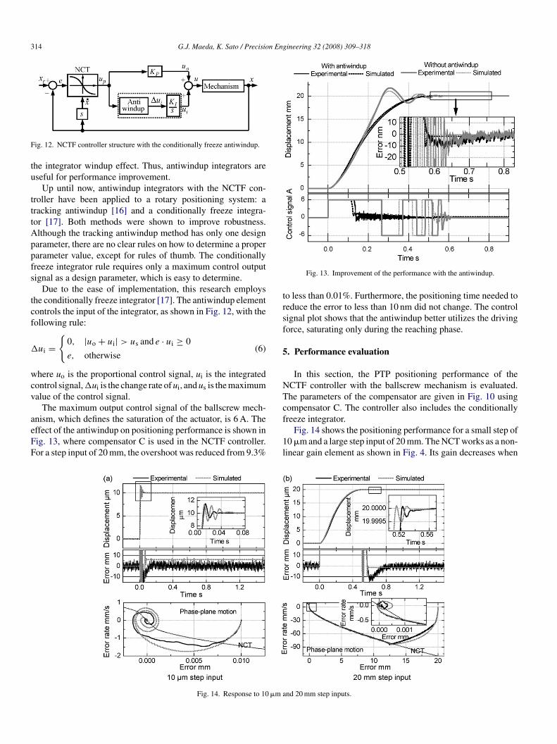
Fig. 14. Response to 10 �m a

Fig. 13. Improvement of the performance with the antiwindup.

o less than 0.01%. Furthermore, the positioning time needed toeduce the error to less than 10 nm did not change. The controlignal plot shows that the antiwindup better utilizes the drivingorce, saturating only during the reaching phase.

. Performance evaluation

In this section, the PTP positioning performance of theCTF controller with the ballscrew mechanism is evaluated.he parameters of the compensator are given in Fig. 10 usingompensator C. The controller also includes the conditionally

reeze integrator.

Fig. 14 shows the positioning performance for a small step of0 �m and a large step input of 20 mm. The NCT works as a non-inear gain element as shown in Fig. 4. Its gain decreases when

nd 20 mm step inputs.

G.J. Maeda, K. Sato / Precision Engineering 32 (2008) 309–318 315

trbTo

1atea

sebbiu1attcotpt

6

tmbaice

Ft

cN

fpespbrgss

upI

6d

Tia

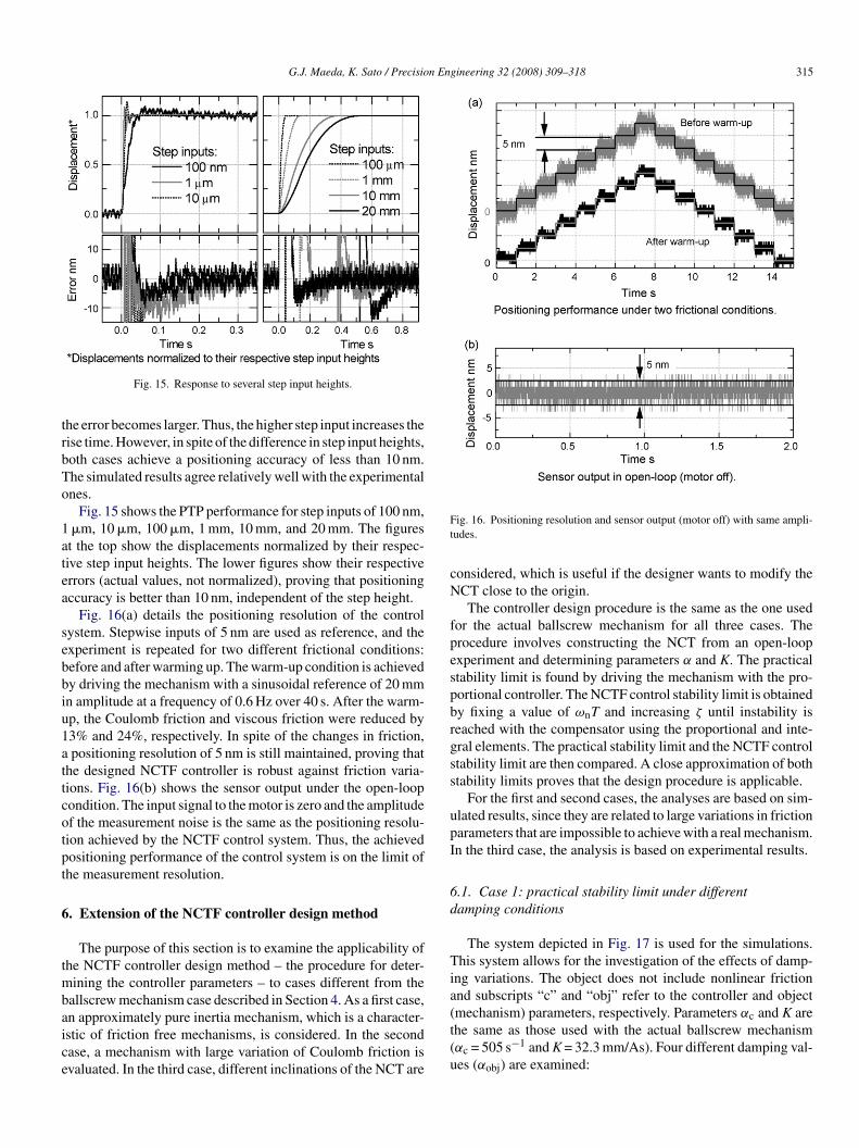
Fig. 15. Response to several step input heights.

he error becomes larger. Thus, the higher step input increases theise time. However, in spite of the difference in step input heights,oth cases achieve a positioning accuracy of less than 10 nm.he simulated results agree relatively well with the experimentalnes.

Fig. 15 shows the PTP performance for step inputs of 100 nm,�m, 10 �m, 100 �m, 1 mm, 10 mm, and 20 mm. The figurest the top show the displacements normalized by their respec-ive step input heights. The lower figures show their respectiverrors (actual values, not normalized), proving that positioningccuracy is better than 10 nm, independent of the step height.

Fig. 16(a) details the positioning resolution of the controlystem. Stepwise inputs of 5 nm are used as reference, and thexperiment is repeated for two different frictional conditions:efore and after warming up. The warm-up condition is achievedy driving the mechanism with a sinusoidal reference of 20 mmn amplitude at a frequency of 0.6 Hz over 40 s. After the warm-p, the Coulomb friction and viscous friction were reduced by3% and 24%, respectively. In spite of the changes in friction,positioning resolution of 5 nm is still maintained, proving that

he designed NCTF controller is robust against friction varia-ions. Fig. 16(b) shows the sensor output under the open-loopondition. The input signal to the motor is zero and the amplitudef the measurement noise is the same as the positioning resolu-ion achieved by the NCTF control system. Thus, the achievedositioning performance of the control system is on the limit ofhe measurement resolution.

. Extension of the NCTF controller design method

The purpose of this section is to examine the applicability ofhe NCTF controller design method – the procedure for deter-

ining the controller parameters – to cases different from theallscrew mechanism case described in Section 4. As a first case,

n approximately pure inertia mechanism, which is a character-stic of friction free mechanisms, is considered. In the secondase, a mechanism with large variation of Coulomb friction isvaluated. In the third case, different inclinations of the NCT are

(t(u

ig. 16. Positioning resolution and sensor output (motor off) with same ampli-udes.

onsidered, which is useful if the designer wants to modify theCT close to the origin.The controller design procedure is the same as the one used

or the actual ballscrew mechanism for all three cases. Therocedure involves constructing the NCT from an open-loopxperiment and determining parameters α and K. The practicaltability limit is found by driving the mechanism with the pro-ortional controller. The NCTF control stability limit is obtainedy fixing a value of ωnT and increasing ζ until instability iseached with the compensator using the proportional and inte-ral elements. The practical stability limit and the NCTF controltability limit are then compared. A close approximation of bothtability limits proves that the design procedure is applicable.

For the first and second cases, the analyses are based on sim-lated results, since they are related to large variations in frictionarameters that are impossible to achieve with a real mechanism.n the third case, the analysis is based on experimental results.

.1. Case 1: practical stability limit under differentamping conditions

The system depicted in Fig. 17 is used for the simulations.his system allows for the investigation of the effects of damp-

ng variations. The object does not include nonlinear frictionnd subscripts “c” and “obj” refer to the controller and objectmechanism) parameters, respectively. Parameters α and K are

che same as those used with the actual ballscrew mechanismαc = 505 s−1 and K = 32.3 mm/As). Four different damping val-es (αobj) are examined:

316 G.J. Maeda, K. Sato / Precision Engineering 32 (2008) 309–318

Fc

ω

espTeu(d

cpdwSbp

tttsot

F

oibζ

6C

Fmfttswif

ig. 17. Sampled-data system used to evaluate the design procedure when αobj

hanges.

.αobj,1 = 0.001 s−1 (approximately a pure inertia mechanism)

.αobj,2 = 250 s−1

.αobj,3 = 505 s−1

.αobj,4 = 750 s−1

The NCTF control stability limit is evaluated at pointsnT = 0.02, 0.1, 0.25, and 0.4 rad.

The results in Fig. 18 show that the practical stability limit forach damping condition is relatively close to the NCTF controltability limit. The average error of approximation between theractical stability limit and the NCTF control stability is 10%.he difference between these stabilities is caused by the integrallement of the NCTF controller, which reduces the ultimate val-es of ζ. Therefore, it is recommended that a margin of safetyat least 10% in this case) is used so that the NCTF control isesigned under the safety area of the practical stability limit.

Fortunately, the NCTF control achieves good positioningharacteristics at values much lower than ζprac. As an exam-le, Fig. 19 shows the simulated results of four control systemsesigned using the system in Fig. 17. In this figure, an objectith αobj,4 was used and the value of ωnT was fixed at 0.25 rad.tep inputs of 1 �m were used. The values of ζ were variedy different margins of safety. It is observed that for a gooderformance, the margins of safety should be larger than 30%.

In the case of the ballscrew mechanism, Fig. 10 shows thathe optimum curve for the design of the controller is 60% lowerhan ζprac (smaller values of margin of safety tend to deterioratehe performance). Therefore, as a practical rule, a margin of

afety for the design should be at least 30%. This value notnly compensates for approximation errors, but also indicateshe region where the control performance is acceptable.

Fig. 18. Practical stability limits under different damping conditions.

ω

wt

eNtpobttpcf

ig. 19. Effects of the margin of safety on relation to the control performance.

The practical stability limit can be used (considering a marginf safety) for mechanisms with different damping values, evenf its variation is large. The result of the condition representedy αobj,1 is especially interesting, because it is an indication thatprac can be used for friction free mechanisms.

.2. Case 2: practical stability limit under differentoulomb friction values

In the second case, the nonlinear model of the mechanism inig. 2(b) is used for the simulations. The characteristics of theechanism model are changed by assigning different Coulomb

riction values. Variations in Coulomb friction occur often, dueo payload variation and lubrication conditions; thus it is impor-ant to examine the feasibility of the practical stability limit inuch cases. The mechanism model is driven in a closed-loopith the NCTF controller in order to find the practical stabil-

ty limit and the NCTF control stability limit. Four Coulombriction values (Tfmax) are examined:

.Tfmax,1 = 0 Nm

.Tfmax,2 = 0.023 Nm

.Tfmax,3 = 0.046 Nm (actual ballscrew mechanism)

.Tfmax,4 = 0.138 Nm

The NCTF control stability limit is evaluated at pointsnT = 0.02, 0.05, 0.1, 0.2, 0.3, and 0.4 rad for the mechanismith Tfmax,3, and at points ωnT = 0.02, 0.1, 0.25 and 0.4 rad for

he other cases.The results in Fig. 20 show the practical stability limit for

ach friction condition, as well as the markers representing theCTF control stability. The average error of approximation in

his case is 16%. The error of approximation shows that theractical stability limit is useful as an indicator for the choicef compensator gains. Although it does not exactly predict theoundary between the unstable and stable regions, it guaran-ees that the stable gains are below ζprac, which greatly helpshe designer when selecting the compensator gains. Thus, the

ractical stability limit is useful as an indicator for the NCTFontroller design for mechanisms subjected to large Coulombriction variations.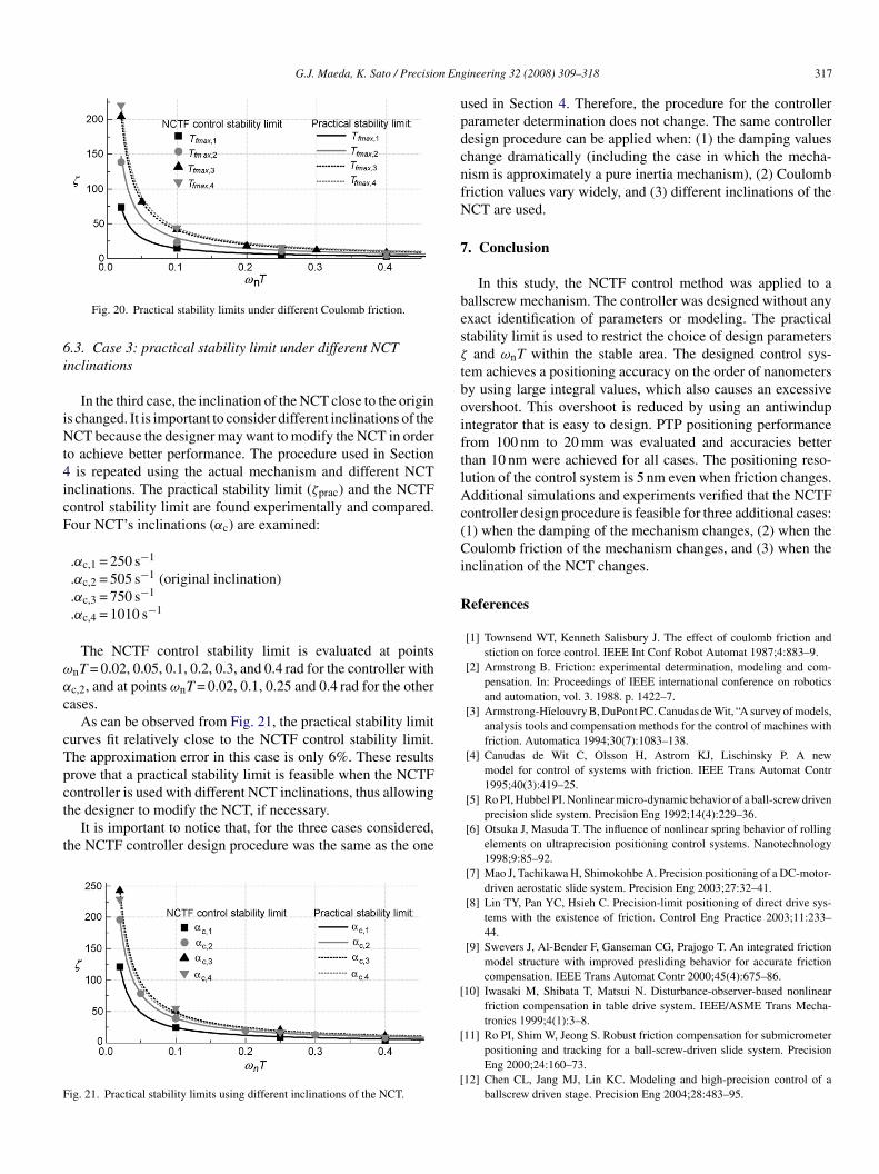

G.J. Maeda, K. Sato / Precision Eng

6i

iNt4icF

ω

α

c

cTpct

t

F

updcnfN

7

besζ

tboiftlAc(Ci

R

Fig. 20. Practical stability limits under different Coulomb friction.

.3. Case 3: practical stability limit under different NCTnclinations

In the third case, the inclination of the NCT close to the origins changed. It is important to consider different inclinations of theCT because the designer may want to modify the NCT in order

o achieve better performance. The procedure used in Sectionis repeated using the actual mechanism and different NCT

nclinations. The practical stability limit (ζprac) and the NCTFontrol stability limit are found experimentally and compared.our NCT’s inclinations (αc) are examined:

.αc,1 = 250 s−1

.αc,2 = 505 s−1 (original inclination)

.αc,3 = 750 s−1

.αc,4 = 1010 s−1

The NCTF control stability limit is evaluated at pointsnT = 0.02, 0.05, 0.1, 0.2, 0.3, and 0.4 rad for the controller withc,2, and at points ωnT = 0.02, 0.1, 0.25 and 0.4 rad for the otherases.

As can be observed from Fig. 21, the practical stability limiturves fit relatively close to the NCTF control stability limit.he approximation error in this case is only 6%. These resultsrove that a practical stability limit is feasible when the NCTF

ontroller is used with different NCT inclinations, thus allowinghe designer to modify the NCT, if necessary.

It is important to notice that, for the three cases considered,he NCTF controller design procedure was the same as the one

ig. 21. Practical stability limits using different inclinations of the NCT.

[

[

[

ineering 32 (2008) 309–318 317

sed in Section 4. Therefore, the procedure for the controllerarameter determination does not change. The same controlleresign procedure can be applied when: (1) the damping valueshange dramatically (including the case in which the mecha-ism is approximately a pure inertia mechanism), (2) Coulombriction values vary widely, and (3) different inclinations of theCT are used.

. Conclusion

In this study, the NCTF control method was applied to aallscrew mechanism. The controller was designed without anyxact identification of parameters or modeling. The practicaltability limit is used to restrict the choice of design parametersand ωnT within the stable area. The designed control sys-

em achieves a positioning accuracy on the order of nanometersy using large integral values, which also causes an excessivevershoot. This overshoot is reduced by using an antiwindupntegrator that is easy to design. PTP positioning performancerom 100 nm to 20 mm was evaluated and accuracies betterhan 10 nm were achieved for all cases. The positioning reso-ution of the control system is 5 nm even when friction changes.dditional simulations and experiments verified that the NCTF

ontroller design procedure is feasible for three additional cases:1) when the damping of the mechanism changes, (2) when theoulomb friction of the mechanism changes, and (3) when the

nclination of the NCT changes.

eferences

[1] Townsend WT, Kenneth Salisbury J. The effect of coulomb friction andstiction on force control. IEEE Int Conf Robot Automat 1987;4:883–9.

[2] Armstrong B. Friction: experimental determination, modeling and com-pensation. In: Proceedings of IEEE international conference on roboticsand automation, vol. 3. 1988. p. 1422–7.

[3] Armstrong-Hıelouvry B, DuPont PC. Canudas de Wit, “A survey of models,analysis tools and compensation methods for the control of machines withfriction. Automatica 1994;30(7):1083–138.

[4] Canudas de Wit C, Olsson H, Astrom KJ, Lischinsky P. A newmodel for control of systems with friction. IEEE Trans Automat Contr1995;40(3):419–25.

[5] Ro PI, Hubbel PI. Nonlinear micro-dynamic behavior of a ball-screw drivenprecision slide system. Precision Eng 1992;14(4):229–36.

[6] Otsuka J, Masuda T. The influence of nonlinear spring behavior of rollingelements on ultraprecision positioning control systems. Nanotechnology1998;9:85–92.

[7] Mao J, Tachikawa H, Shimokohbe A. Precision positioning of a DC-motor-driven aerostatic slide system. Precision Eng 2003;27:32–41.

[8] Lin TY, Pan YC, Hsieh C. Precision-limit positioning of direct drive sys-tems with the existence of friction. Control Eng Practice 2003;11:233–44.

[9] Swevers J, Al-Bender F, Ganseman CG, Prajogo T. An integrated frictionmodel structure with improved presliding behavior for accurate frictioncompensation. IEEE Trans Automat Contr 2000;45(4):675–86.

10] Iwasaki M, Shibata T, Matsui N. Disturbance-observer-based nonlinearfriction compensation in table drive system. IEEE/ASME Trans Mecha-tronics 1999;4(1):3–8.

11] Ro PI, Shim W, Jeong S. Robust friction compensation for submicrometerpositioning and tracking for a ball-screw-driven slide system. PrecisionEng 2000;24:160–73.

12] Chen CL, Jang MJ, Lin KC. Modeling and high-precision control of aballscrew driven stage. Precision Eng 2004;28:483–95.

3 n En

[

[

[

[

[

[

[

[

[tioning mechanism with friction. Precision Eng 2004;28:426–34.

18 G.J. Maeda, K. Sato / Precisio

13] Otsuka J. Nanometer level positioning using three kinds of lead screws.Nanotechnology 1992;3:29–36.

14] Otsuka J, Ichikawa S, Masuda T, Suzuki K. Development of a small ultra-precision positioning device with 5 nm resolution. Measure Sci Technol2005;16:2186–92.

15] Wahyudi, Sato K, Shimokohbe A. Characteristics of practical controlfor point-to-point (PTP) positioning systems effect of design parame-ters and actuator saturation on positioning performance. Precision Eng2003;27:157–69.

16] Wahyudi, Albagul A. Performance improvement of practical controlmethod for positioning systems in the presence of actuator saturation. In:

Proceedings of the 2004 IEEE international conference on control applica-tions. 2004. p. 296–302.

17] Sato K. Robust and practical control for PTP positioning. In: Proceedingsof the first international conference on positioning technology. 2004. p.394–5.

[

[

gineering 32 (2008) 309–318

18] Wahyudi, Sato K, Shimokohbe A. Robustness evaluation of new practi-cal control for PTP positioning systems. In: International conference onadvanced intelligent mechatronics proceedings. 2001. p. 843–8.

19] Wahyudi. Robustness evaluation of two control methods for friction com-pensation of PTP positioning systems. In: Proceedings of 2003 IEEEconference on control applications. 2003. p. 1454–8.

20] Wahyudi, Sato K, Shimokohbe A. Robustness evaluation of three fric-tion compensation methods for point-to-point (PTP) systems. RobotAutonomous Syst 2005;52:247–56.

21] Sato K, Nakamoto K, Shimokohbe A. Practical control of precision posi-

22] Wahyudi, New practical control of PTP positioning systems. PhD Thesis.Tokyo Institute of Technology; 2002.

23] Franklin GF, Powell JD, Workman ML. Digital control of dynamic systems.2nd ed. Addison Wesley; 1990.