practical interpretation of rasp charts (blipmaps) · practical interpretation of rasp charts...

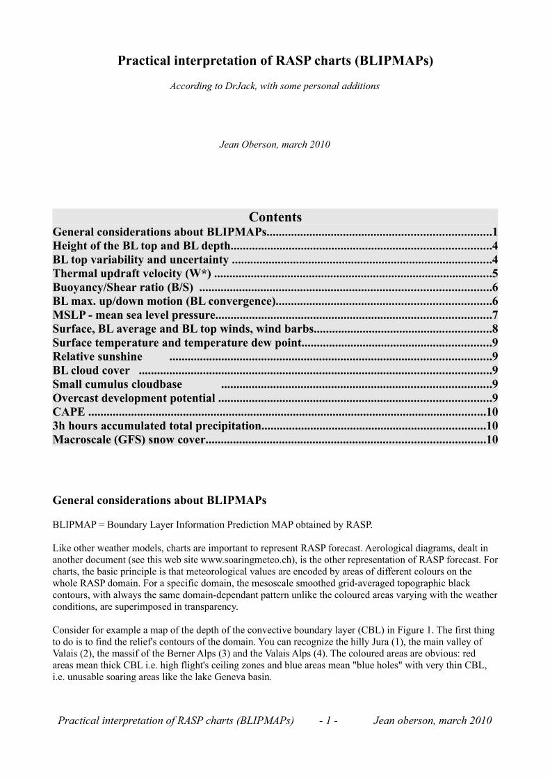
Practical interpretation of RASP charts (BLIPMAPs)

According to DrJack, with some personal additions

Jean Oberson, march 2010

ContentsGeneral considerations about BLIPMAPs.........................................................................1Height of the BL top and BL depth.....................................................................................4BL top variability and uncertainty .....................................................................................4Thermal updraft velocity (W*) ...........................................................................................5Buoyancy/Shear ratio (B/S) ...............................................................................................6BL max. up/down motion (BL convergence)......................................................................6MSLP - mean sea level pressure..........................................................................................7Surface, BL average and BL top winds, wind barbs..........................................................8Surface temperature and temperature dew point..............................................................9Relative sunshine .........................................................................................................9BL cloud cover ...................................................................................................................9Small cumulus cloudbase ........................................................................................9Overcast development potential .........................................................................................9CAPE ..................................................................................................................................103h hours accumulated total precipitation.........................................................................10Macroscale (GFS) snow cover...........................................................................................10

General considerations about BLIPMAPs

BLIPMAP = Boundary Layer Information Prediction MAP obtained by RASP.

Like other weather models, charts are important to represent RASP forecast. Aerological diagrams, dealt in another document (see this web site www.soaringmeteo.ch), is the other representation of RASP forecast. For charts, the basic principle is that meteorological values are encoded by areas of different colours on the whole RASP domain. For a specific domain, the mesoscale smoothed grid-averaged topographic black contours, with always the same domain-dependant pattern unlike the coloured areas varying with the weather conditions, are superimposed in transparency.

Consider for example a map of the depth of the convective boundary layer (CBL) in Figure 1. The first thing to do is to find the relief's contours of the domain. You can recognize the hilly Jura (1), the main valley of Valais (2), the massif of the Berner Alps (3) and the Valais Alps (4). The coloured areas are obvious: red areas mean thick CBL i.e. high flight's ceiling zones and blue areas mean "blue holes" with very thin CBL, i.e. unusable soaring areas like the lake Geneva basin.

Practical interpretation of RASP charts (BLIPMAPs) - 1 - Jean oberson, march 2010

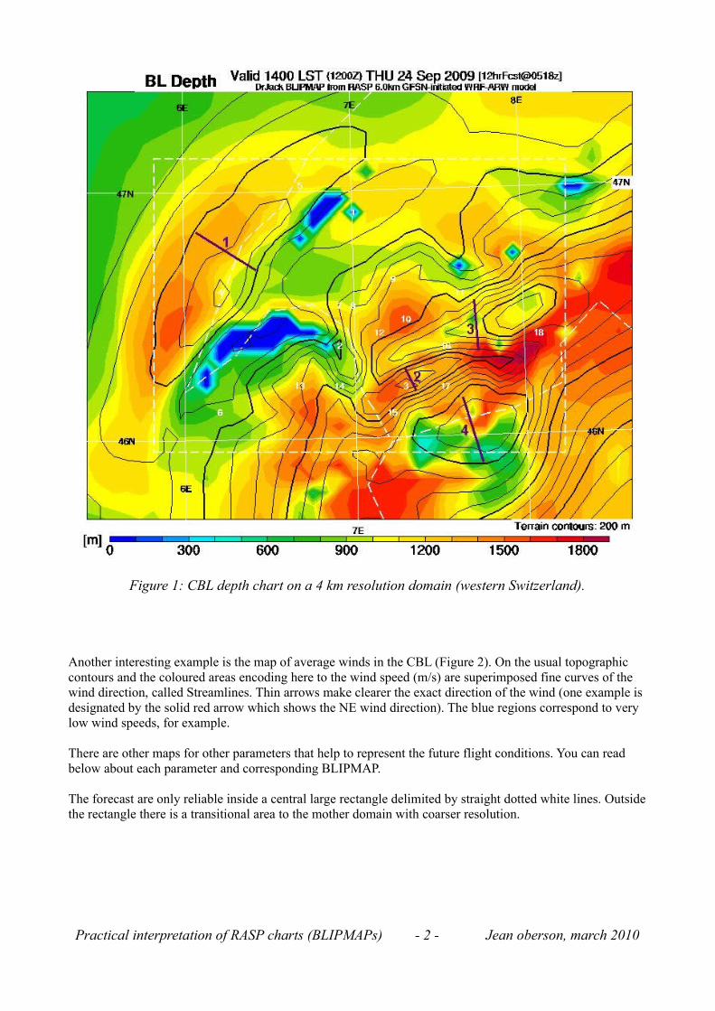
Figure 1: CBL depth chart on a 4 km resolution domain (western Switzerland).

Another interesting example is the map of average winds in the CBL (Figure 2). On the usual topographic contours and the coloured areas encoding here to the wind speed (m/s) are superimposed fine curves of the wind direction, called Streamlines. Thin arrows make clearer the exact direction of the wind (one example is designated by the solid red arrow which shows the NE wind direction). The blue regions correspond to very low wind speeds, for example.

There are other maps for other parameters that help to represent the future flight conditions. You can read below about each parameter and corresponding BLIPMAP.

The forecast are only reliable inside a central large rectangle delimited by straight dotted white lines. Outside the rectangle there is a transitional area to the mother domain with coarser resolution.


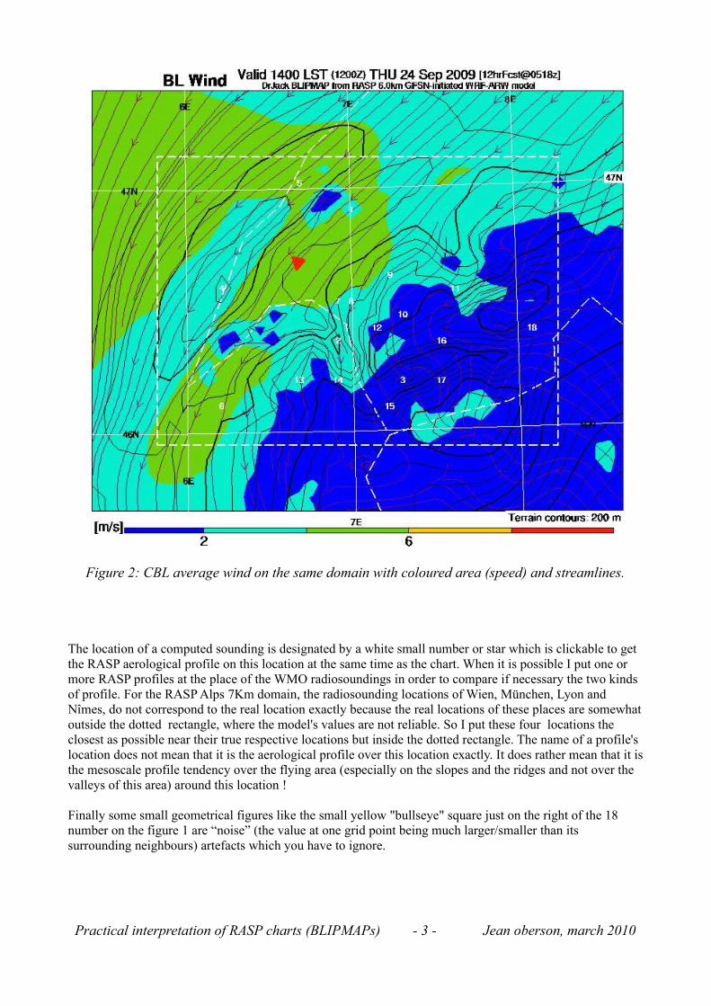
Figure 2: CBL average wind on the same domain with coloured area (speed) and streamlines.

The location of a computed sounding is designated by a white small number or star which is clickable to get the RASP aerological profile on this location at the same time as the chart. When it is possible I put one or more RASP profiles at the place of the WMO radiosoundings in order to compare if necessary the two kinds of profile. For the RASP Alps 7Km domain, the radiosounding locations of Wien, München, Lyon and Nîmes, do not correspond to the real location exactly because the real locations of these places are somewhat outside the dotted rectangle, where the model's values are not reliable. So I put these four locations the closest as possible near their true respective locations but inside the dotted rectangle. The name of a profile's location does not mean that it is the aerological profile over this location exactly. It does rather mean that it is the mesoscale profile tendency over the flying area (especially on the slopes and the ridges and not over the valleys of this area) around this location !

Finally some small geometrical figures like the small yellow "bullseye" square just on the right of the 18 number on the figure 1 are “noise” (the value at one grid point being much larger/smaller than its surrounding neighbours) artefacts which you have to ignore.


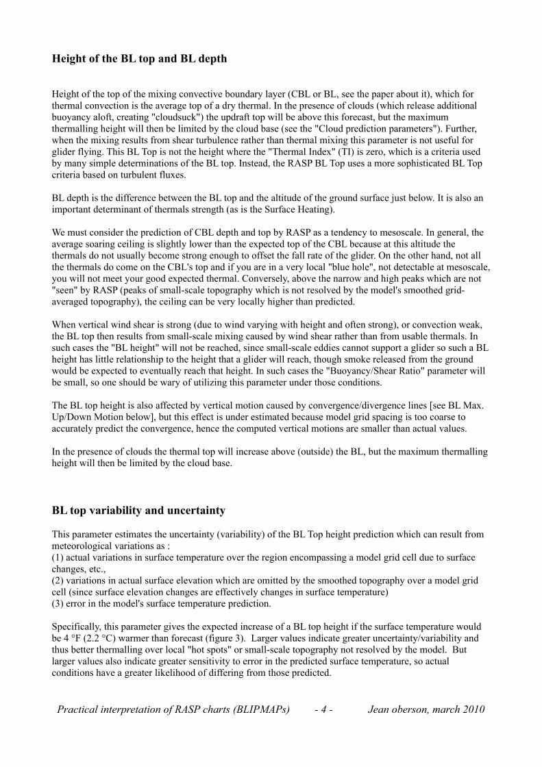
Height of the BL top and BL depth

Height of the top of the mixing convective boundary layer (CBL or BL, see the paper about it), which for thermal convection is the average top of a dry thermal. In the presence of clouds (which release additional buoyancy aloft, creating "cloudsuck") the updraft top will be above this forecast, but the maximum thermalling height will then be limited by the cloud base (see the "Cloud prediction parameters"). Further, when the mixing results from shear turbulence rather than thermal mixing this parameter is not useful for glider flying. This BL Top is not the height where the "Thermal Index" (TI) is zero, which is a criteria used by many simple determinations of the BL top. Instead, the RASP BL Top uses a more sophisticated BL Top criteria based on turbulent fluxes.

BL depth is the difference between the BL top and the altitude of the ground surface just below. It is also an important determinant of thermals strength (as is the Surface Heating).

We must consider the prediction of CBL depth and top by RASP as a tendency to mesoscale. In general, the average soaring ceiling is slightly lower than the expected top of the CBL because at this altitude the thermals do not usually become strong enough to offset the fall rate of the glider. On the other hand, not all the thermals do come on the CBL's top and if you are in a very local "blue hole", not detectable at mesoscale, you will not meet your good expected thermal. Conversely, above the narrow and high peaks which are not "seen" by RASP (peaks of small-scale topography which is not resolved by the model's smoothed grid-averaged topography), the ceiling can be very locally higher than predicted.

When vertical wind shear is strong (due to wind varying with height and often strong), or convection weak, the BL top then results from small-scale mixing caused by wind shear rather than from usable thermals. In such cases the "BL height" will not be reached, since small-scale eddies cannot support a glider so such a BL height has little relationship to the height that a glider will reach, though smoke released from the ground would be expected to eventually reach that height. In such cases the "Buoyancy/Shear Ratio" parameter will be small, so one should be wary of utilizing this parameter under those conditions.

The BL top height is also affected by vertical motion caused by convergence/divergence lines [see BL Max. Up/Down Motion below], but this effect is under estimated because model grid spacing is too coarse to accurately predict the convergence, hence the computed vertical motions are smaller than actual values.

In the presence of clouds the thermal top will increase above (outside) the BL, but the maximum thermalling height will then be limited by the cloud base.

BL top variability and uncertainty This parameter estimates the uncertainty (variability) of the BL Top height prediction which can result from meteorological variations as : (1) actual variations in surface temperature over the region encompassing a model grid cell due to surface changes, etc., (2) variations in actual surface elevation which are omitted by the smoothed topography over a model grid cell (since surface elevation changes are effectively changes in surface temperature) (3) error in the model's surface temperature prediction.

Specifically, this parameter gives the expected increase of a BL top height if the surface temperature would be 4 °F (2.2 °C) warmer than forecast (figure 3). Larger values indicate greater uncertainty/variability and thus better thermalling over local "hot spots" or small-scale topography not resolved by the model. But larger values also indicate greater sensitivity to error in the predicted surface temperature, so actual conditions have a greater likelihood of differing from those predicted.


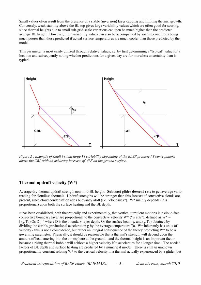
Small values often result from the presence of a stable (inversion) layer capping and limiting thermal growth. Conversely, weak stability above the BL top gives large variability values which are often good for soaring, since thermal heights due to small sub-grid-scale variations can then be much higher than the predicted average BL height. However, high variability values can also be accompanied by soaring conditions being much poorer than those predicted if actual surface temperatures are much cooler than those predicted by the model.

This parameter is most easily utilized through relative values, i.e. by first determining a "typical" value for a location and subsequently noting whether predictions for a given day are for more/less uncertainty than is typical.

Figure 2 : Example of small Vs and large Vl variability depending of the RASP predicted T curve pattern above the CBL with an arbitrary increase of 4°F on the ground surface.

Thermal updraft velocity (W*)

Average dry thermal updraft strength near mid-BL height. Subtract glider descent rate to get average vario reading for cloudless thermals. Updraft strengths will be stronger than this forecast if convective clouds are present, since cloud condensation adds buoyancy aloft (i.e. "cloudsuck"). W* mainly depends (it is proportional) upon both the surface heating and the BL depth.

It has been established, both theoretically and experimentally, that vertical turbulent motions in a cloud-free convective boundary layer are proportional to the convective velocity W* ("w star"), defined as W* = [ (g/To) Qs D ]1/3 where D is the boundary layer depth, Qs the surface heating, and (g/To) obtained by dividing the earth's gravitational acceleration g by the average temperature To. W* inherently has units of velocity - this is not a coincidence, but rather an integral consequence of the theory predicting W* to be a governing parameter. Physically, it should be reasonable that a thermal's strength will depend upon the amount of heat entering into the atmosphere at the ground - and the thermal height is an important factor because a rising thermal bubble will achieve a higher velocity if it accelerates for a longer time. The needed factors of BL depth and surface heating are predicted by a numerical model. There is still an unknown proportionality constant relating W* to the vertical velocity in a thermal actually experienced by a glider, but


by theory that constant is not completely arbitrary - it should be approximately one, with the exact value depending upon such factors as the area over which the vertical velocity is averaged (since a thermal's core is stronger than its periphery) and thus will depend upon the thermalling radius of the glider, for example. For now I have simply set this proportionality factor to one and it is gratifying to find that without having to resort to any empiricism whatsoever the predicted vertical velocities are quantitatively very realistic. With further experience the proportionality constant might be adjusted slightly, but the present results are considered very reasonable, given that a range of thermal strengths occur at any one time and that vertical velocity of a thermal will vary both with height and with distance from the core. And adding besides, W* - like all model parameters - is best evaluated relatively than as an precise value. W* follows the pilot's rule that deep thermals tend to be strong thermals, but also includes the influence of surface heating. If convective clouds are present, the actual W* will be probably larger than calculated here due to the "cloudsuck".

Buoyancy/Shear ratio (B/S) Dry thermals may be broken up by vertical wind shear (i.e. wind changing with height) and unworkable if B/S ratio is 5 or less. If convective clouds are present, the actual B/S ratio will be larger than calculated here due to the "cloudsuck". This parameter is truncated at 20 for plotting.

The BL top height prediction indicates the height to which mixing will occur but not all mixing is equally useful to glider pilots. Mixing can be produced both by thermals and by (vertical) wind shear, but only thermals produce the relatively large updrafts needed for soaring. To help evaluate the degree to which the day's mixing is convectively driven, The "B/S" parameter represents the ratio between Buoyancy and Shear production of turbulence. A small Buoyancy/Shear Ratio (B/S) B/S value indicates wind shear, due to wind changing with height, is likely a significant problem - at present the best guidance I have, based upon sailplane pilot reports, is that on days with B/S of 5 or less the thermals are likely to be too broken to be usable - hang gliders and paragliders, who are able to turn in smaller circles, seem to be able to thermal in smaller values, based on a few reports I have received. At a B/S of 10 or above, vertical shear is likely not a significant factor. Note that only a single value is provided, representing the BL as a whole, whereas B/S normally decreases closer to the surface.

The B/S ratio is not an empirical approach but is based upon the non-dimensional number used to distinguish between "buoyancy dominated" and "shear dominated" BLs (and those in between). It is the ratio of the "buoyant production of turbulent kinetic energy" to the "shear production of turbulent kinetic energy" with both being well defined terms. However, the cross-over criterion between "workable" and "unworkable" thermals must be determined empirically (and for that matter there is no sharp cut-off between the two cases).

In short, B/S parameter corresponds to the quality of the thermals which is as important as their vertical extension or their updraft velocity.

BL max. up/down motion (BL convergence)

Maximum grid-area-averaged extensive upward or downward motion within the BL as created by horizontal wind convergence. Positive convergence is associated with local convergence lines which are horizontal changes of wind speed/direction. However, the actual size of such features is usually smaller than can be resolved by the model so only stronger ones will be forecast and their predictions are subject to much error. If CAPE is also large, thunderstorms can be triggered. Negative convergence (divergence) produces subsiding vertical motion, creating low-level inversions which limit thermalling heights. This parameter can be noisy, so users should be wary. For a grid resolution of 12km or better convergence lines created by terrain are commonly predicted - sea-breeze predictions can also be found for strong cases, though they are best resolved by smaller-resolution grids.


MSLP - mean sea level pressure

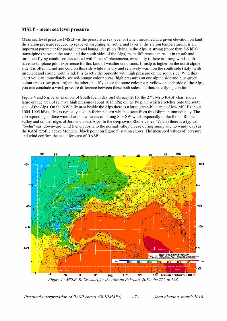
Mean sea level pressure (MSLP) is the pressure at sea level or (when measured at a given elevation on land) the station pressure reduced to sea level assuming an isothermal layer at the station temperature. It is an important parameter for paraglider and hangglider pilots flying in the Alps. A strong (more than 3-5 hPa) transalpine (between the north and the south sides of the Alps) mslp difference can result in unsafe and turbulent flying conditions associated with “foehn” phenomena, especially if there is strong winds aloft. I have no sailplane pilot experience for this kind of weather conditions. If mslp is higher on the north alpine side it is often humid and cold on this side while it is dry and relatively warm on the south side (Italy) with turbulent and strong north wind. It is exactly the opposite with high pressure on the south side. With this chart you can immediately see red-orange colour areas (high pressure) on one alpine side and blue-green colour areas (low pressure) on the other one. If you see the same colour e.g. yellow on each side of the Alps, you can conclude a weak pressure difference between these both sides and thus safe flying conditions

Figure 4 and 5 give an example of South foehn day on February 2010, the 27th. Mslp RASP chart shows large orange area of relative high pressure (about 1013 hPa) on the Pô plain which stretches onto the south side of the Alps. On the NW hilly area beside the Alps there is a large green-blue area of low MSLP (about 1004-1005 hPa). This is typically a south foehn pattern which is seen from this Blipmap immediately. The corresponding surface wind chart shows areas of strong S or SW winds especially in the french Rhone valley and on the ridges of Jura and swiss Alps. In the deep swiss Rhone valley (Valais) there is a typical “foehn” east downward wind (i.e. Opposite to the normal valley breeze during sunny and no windy day) as the RASP profile above Montana (black point on figure 5) station shows. The measured values of pressure and wind confirm the exact forecast of RASP.

Figure 4 : MSLP RASP chart for the Alps on February 2010, the 27th, at 12Z.


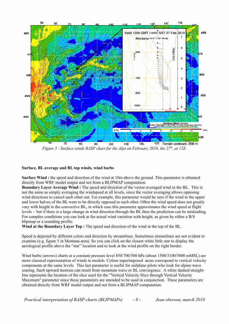
Figure 5 : Surface winds RASP chart for the Alps on February 2010, the 27th, at 12Z.

Surface, BL average and BL top winds, wind barbs

Surface Wind : the speed and direction of the wind at 10m above the ground. This parameter is obtained directly from WRF model output and not from a BLIPMAP computation. Boundary Layer Average Wind : The speed and direction of the vector-averaged wind in the BL. This is not the same as simply averaging the windspeed at all levels, since the vector averaging allows opposing wind directions to cancel each other out. For example, this parameter would be zero if the wind in the upper and lower halves of the BL were to be directly opposed to each other. Often the wind speed does not greatly vary with height in the convective BL, in which case this parameter approximates the wind speed at flight levels - but if there is a large change in wind direction through the BL then the prediction can be misleading. For complex conditions you can look at the actual wind variation with height, as given by either a B/S blipmap or a sounding profile.Wind at the Boundary Layer Top : The speed and direction of the wind at the top of the BL.

Speed is depicted by different colors and direction by streamlines. Sometimes streamlines are not evident to examine (e.g. figure 5 in Montana area). So you can click on the closest white little star to display the aerological profile above the “star” location and to look at the wind profile on the right border.

Wind barbs (arrows) charts at a constant pressure level 850/700/500 hPa (about 1500/3100/5800 mMSL) are more classical representation of winds in models. Colour superimposed areas correspond to vertical velocity components at the same levels. This last parameter is useful for sailplane pilots who look for alpine wave soaring. Such upward motions can result from mountain wave or BL convergence. A white dashed straight-line represents the location of the slice used for the "Vertical Velocity Slice through Vertical Velocity Maximum" parameter since these parameters are intended to be used in conjunction. These parameters are obtained directly from WRF model output and not from a BLIPMAP computation.


Surface temperature and temperature dew point The temperature T or the dew point temperature Td at a height of 2m above ground level. This can be compared to observed surface T and Td as an indication of model simulation accuracy; e.g. if observed surface T are significantly below those forecast, then soaring conditions will be poorer than forecast and if observed surface Td are significantly below those forecast, then BL cloud formation will be poorer than forecast. These parameters are obtained directly from WRF model output and not from a RASP-BLIPMAP computation.

Relative sunshine

It is the surface sunshine normalized (divided) by the amount of solar radiation which would reach the surface in a dry atmosphere (i.e. in the absence of clouds and water vapor), expressed as a percentage. This parameter indicates the degree of cloudiness, i.e. where clouds limit the sunlight reaching the surface. So if there is 100% of dense clouds, the relative sunshine will be 0%. With 25% of such clouds, it will be 75%, but with 100% of half dense translucent clouds, it will be about 50%. This parameter can therefore often seem to over-evaluate the sunshine due to its translucency evaluation. Sometimes I have experimented (observed) a whole covered sky with no subjective feeling of significant translucency whereas RASP forecast some significant degree of sunshine !

BL cloud cover This parameter evaluates the formation of clouds (cu, sc, st) within the BL. It assumes a simple relationship between cloud cover percentage and the maximum relative humidity within the BL. The cloud base height is not predicted, but is expected to be below the BL Top height.

Small cumulus cloudbase

This height estimates the mesoscale cloudbase for small, non-extensive "puffy" cumulus in the BL only at locations (coloured areas on BLIPMAP charts) where this cumulus formation is probable. Where these clouds are not probable the areas remain grey. Nevertheless cumulus can even occur on grey areas if the air is lifted up the indicated vertical distance by flow up a small-scale ridge not resolved by the model's smoothed topography.

Overcast development potential

This evaluates the potential for extensive cloud formation (Overcast development = OD) at the BL top. Likely OD is predicted when the parameter is positive, with OD being increasingly more likely with higher positive values. OD can also occur with small negative values if the air is lifted up the indicated vertical distance by flow up a small-scale ridge not resolved by the model's smoothed topography. This parameter is truncated at -10,000 for plotting. Empirical evaluation of OD Potential predictions vs. actual OD experience and use of an empirical criterion different from zero may yield better results at your location. Note that in some cases only negative numbers may appear in the colorbar legend, in which case the statement "OvercastDevelopment being increasingly more likely with higher positive values" should be read as "OvercastDevelopment being increasingly more likely with less negative vales".


CAPE

CAPE (Convective Available Potential Energy) is a measure of the atmospheric stability affecting deep convective cloud formation above the CBL and not inside CBL. So it is not a measure of the strength of thermals. Higher values indicates greater potential for strong thunderstorm. Thunderstorm probabilities according to CAPE values are:

0=none, 300-1000=weak, 1000-2500=moderate, 2500-5300=strong.

This parameter only indicates the potential for thunderstorm formation - for thunderstorms to actually form also requires some triggering mechanism which produces upward motion, such as flow over a ridge or convergence. This parameter is obtained directly from model output and not from a BLIPMAP computation.

3h hours accumulated total precipitation

This is the accumulation in mm of all kinds of water precipitation during the last 3 hours at 9Z, 12Z and 15Z.. For RASP of the Alps for example it covers only form 6Z to 15Z.

Macroscale (GFS) snow cover

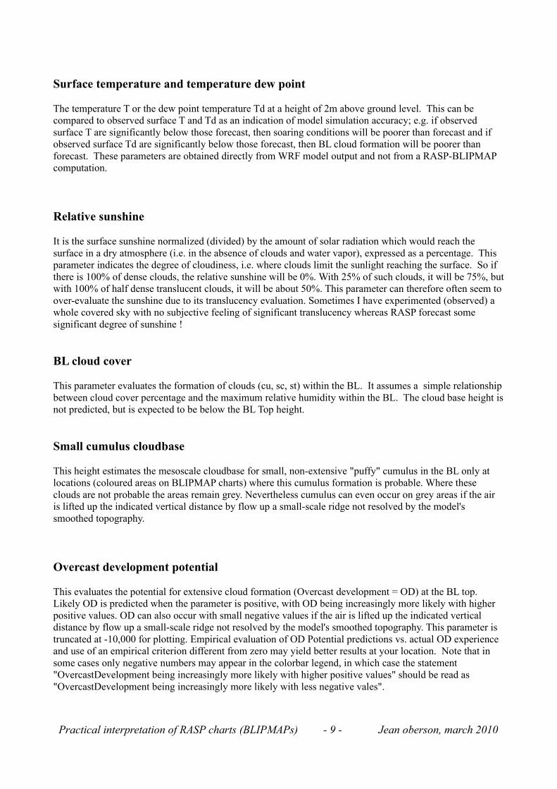
This macroscale snow cover chart is showed in order to explain (warn) a potential serious limitation of RASP. Purple areas mean the ground surface is simply covered with snow without taking account of the thickness of snow. Blue areas mean region without snow.

The forecast problem can be traced to input from the driving global GFS model, with too large snow region over the Alps at macroscale (GFS model view). Naturally if RASP is told there is snow cover it is not going to predict any thermals, and other predictions which depend upon surface heating will also be incorrect. The probable reason for the anomalously-predicted snow is that GFS uses "envelope topography" which for terrain values uses the maximum elevation in a grid cell rather than the average, which would produce a large area of higher-than-actual elevations and hence more snow than is actually the case. "Envelope topography" tends to produce better "dynamics", such as wind predictions, but at the cost of poorer thermodynamics, such as surface temperatures. And because the grid cell of macroscale GFS is around 50km, any such anomaly is spread over many points in the RASP grid. It is an example of a case in which RASP forecasts can be invalid due to its dependence upon forecasts from the global model. To alleviate this anomaly I "tell" to my Alps RASP model before it runs that there no snow in winter and in the beginning of spring when there has been no new snow fall for a few day, because in this case I empirically notice that probably the heating effect of snow-free alpine pine forest is not negligible in the alpine valley. When just new snow falls, the pine forest is also covered by snow (it is of course beautiful) but there is no significant heating source, so I “tell” to the model to put the snow cover parameter on.

Figure 6 below, shows a concrete example of this problem. The south french Provence, famous for its warm climate, has a snow-free ground surface on march, what is very usual and what is seen on the satellite image. Nevertheless the GFS model considers that this area is covered by snow down to the mediterranean sea border !! For the broad and deep Bolzano valley and the large swiss Rhone valley (Valais) one can see the same discrepancy between the model snow cover chart and the satellite image. Moreover, even in the high small valleys, the pine forests during winter seem to be non negligible for the CBL thermodynamics, especially when they are not covered by new snow. In winter and at the beginning of spring, pilots usually do not fly on the high snow covered peaks but instead on the snow-free valley slopes. That is why I can


empirically “cheat” and “tell” RASP there is no snow in these conditions.

Figure 6 : discrepancy between macroscale RASP snow cover and real snow cover as seen on a sat image (on the right) at about the same time on the Alps (2010, 5th march). 1 = Bolzano valley. 2 = Provence. 3 = Valais. There are still some superimposed numerous cumulus which increase the size of the white areas on the sat image. Therefore the real snow cover should be still less spread.


practical interpretation of rasp charts (blipmaps) · practical interpretation of rasp charts...

Documents