—

—

oad surface by the vehicle’s tires. There are

–

Weigh-In-Motion System in Flexible Pavements Using Fiber Bragg Grating Sensors Part A: Concept

Mu’ath Al

Pre-Print Manuscript:Al-Tarawneh, M., Huang, Y., Lu, P., Bridgelall, R. (2019). Weigh-In-Motion System in Flexible Pavements Using Fiber Bragg Grating Sensors Part A: Concept. Transactions on Intelligent Transportation Systems. DOI: 10.1109/TITS.2019.2949242, pp. 1-12.

-Tarawneh, Ying Huang*, Pan Lu, and Raj Bridgelall

Abstract Weight data of vehicles play an important role in traffic planning, weight enforcement, and pavement condition assessment. In this paper, a weigh-in-motion (WIM) system that functions at both low-speeds and high-speeds in flexible pavements is developed based on in-pavement, three-dimensional glass-fiber­reinforced, polymer-packaged fiber Bragg grating sensors (3D GFRP-FBG). Vehicles passing over the pavement produce strains that the system monitors by measuring the center wavelength changes of the embedded 3D GFRP-FBG sensors. The FBG sensor can estimate the weight of vehicles because of the direct relationship between the loading on the pavement and the strain inside the pavement. A sensitivity study shows that the developed sensor is very sensitive to sensor installation depth, pavement property, and load location. Testing in the field validated that the longitudinal component of the sensor if not corrected by location has a measurement accuracy of86.3% and 89.5% at 5 mph and 45 mph vehicle speed, respectively. However, the system also has the capability to estimate the location of the loading position, which can enhance the system accuracy to more than 94.5'1/o.

Index Terms weigh in motion (WIM), fiber Bragg grating sensor, sensitivity study, flexible pavement.

I. INTRODUCTION

ESTIMATION of vehicle weight is a controlling factor in flexible pavement design, which has a significant effect on

road maintenance costs and the safety of road users. The flexible pavement experiences dynamic loads rather than static weights that pavement design guides use. One example is the American Association of State Highway and Transportation Officials (AASHTO) which uses equivalent single axle loads (ESAL), a static weight measurement, to represent vehicle loads in its pavement design guide [1]. Currently, new methods, such as the Mechanistic Empirical Pavement Design Guide (MEPDG) use axle load spectra to represent vehicle loads in pavement design [2]. Hence, it has become very important to monitor real-time dynamic loads from vehicles in the field.

Traditionally, law enforcement collects the weights of vehicles by pulling them off the roadway and weighing them at weigh stations while the vehicles are at rest. These stationary scales have some limitations: they are time-consuming, taking approximately 5 minutes to weigh each truck; they have limited space, usually accommodating about 15 trucks at a time [3]; there is potential to miss overloaded trucks [4]; and weigh stations pose accident hazards because of stopped vehicles on the weight station entrance. Thus, the weigh-in-motion (WIM) systems are developing quickly as pre-selection systems for assisting static weight stations.

The concept of WIM was introduced more than 50 years ago [5]. The literature defines WIM as a process for estimating the

Mu'ath Al-Tarawneh, and Ying Huang* are in the department of Civil and Environmental Engineering, North Dakota State University, USA.

static weight of a vehicle by calculating the dynamic load applied to the r several advantages of WIM system over the stationary weight scale, including savings in time and cost, and the ability to collect continuous traffic data without human intervention. Generally, there are two types of WIM systems: low-speed WIM (LSWIM) for vehicle speeds of up to 25 mph, and high­speed WIM (HSWIM) for vehicle speeds of up to 80 mph. Agencies usually apply LSWIM sensors in combination with stationary weight scales for weight enforcement purposes and pavement design and maintenance. With growing demand to collect real traffic data and weight information, especially after the introduction of weigh-station bypass programs, there is a greater need for a HSWIM system.

An effective WIM system includes at least three components: a network of in-pavement sensors, a facility for data acquisition, and an algorithm or framework for WIM data extraction. In general, there are several types of in-pavement sensors for WIM applications, including bending plates, piezoelectric sensors, and load cells [6-8]. Table I compares the cost, sensitivity, error source, and life cycle for various current common WIM sensors. For piezoelectric sensors, they can either be made by quartz or polymer. The piezoelectric sensor has higher measurement accuracy for WIM measurements compared with polymer piezoelectric sensors and insensitive to the temperature, but still has higher initial and installing cost ($ 14,000 per lane) [9]. In general, the common electrical sensors (piezoelectric sensor, bending plate, and load cell) showed a significant dependence on the surrounding environmental factors, such as moisture. They also showed high levels of electromagnetic interference (EMI) and relatively short life cycles with moderate error.

TABLE I WIM SENSOR COMPARISON [6] [IO]

Piezoelectric Bending Single sensor plate load cell

Annual life Low Medium High cycle cost ($ 5,000) ($6,000) ($ 8,000)

Error +/- 15% +/-10% +/-6%

Sensitivity High Medium Low

Expected life 4 years 6 years 12 years

To overcome the drawbacks of the current common WIM sensors, optic fiber sensors [10] have been attracted the attention from researchers due to their unique advantages of compactness, high sensitivity, immunity to electromagnetic interference (EMI) and moisture, capability of quasi-distributed sensing, low cost ofless $1,000, easy installation in a few hours, and long life cycles [11, 12]. Optic fiber sensors have great

Pan Lu and Raj Bridgelall are in Upper Great Plains Transportation Institute (UGPTI), North Dakota State University, USA.

* Corresponding author: ying.huang@ndsu.edu

author’s research team

’s

per as “Part A” of this study will introduce

and a further “Part B”

L=l

Λ

Λε. The

D++-=D

+D

=D

gael

l

l

l

l

l

e

e

D+=D

=D

gal

l

l

l

a g

λ

λ

affect the fiber’s elasto

l

l

l

le

D-

D

-=

authors’ research group [1

potential to be a long-term and reliable solution for detecting WIM in real time.

Among fiber optic sensors, the fiber Bragg grating (FBG) sensor is the one most commonly used for civil engineering applications and has been widely used in field applications to measure temperature, strains, and loads [9-10]. However, the installation process may easily damage the sensor because the construction of FBG contains silica material. Thus, the packaging is necessary for FBGs in any field applications. Glass-fiber-reinforced polymer (GFRP) material provides durable and reliable packaging which has become widely accepted for use in civil engineering applications [13]. Hence, researchers used the GFRP material to package a three­dimension (3D) FBG sensor to improve its ruggedness. The

introduced the 3D GFRP-FBG sensor for a pavement health monitoring system [14] , [15], and LSWIM system in rigid pavements [16].

This study installed the 3D GFRP-FBG sensor into flexible pavements to serve as a WIM system at both low and high vehicle speed ofup to 45 mph. In this paper, the authors explain the sensor operational principle and design and contribute a systematic sensitivity study along with a case study of testing in the field. This pa the concept of the 3D GFRP-FBG sensor for WIM measurements in flexible pavements study will focus on parametric study on all the influencing factors to reduce the measurement error of the system. Thus, the organization of the remainder of this paper is as follows : Section 2 introduces the sensor operational principle and sensor design; Section 3 shows the sensitivity study of the GFRP-FBG sensors for WIM measurement using theoretical analysis; Section 4 describes the field-testing validation and discussion. Finally, Section 5 concludes the study and suggests future work.

II. OPERATIONAL PRINCIPLE AND SENSOR DESIGN

A. Operational principle of the FBG sensor

The formation of FBG in an optical fiber was first demonstrated by Hill et al. in 1978 at the Canadian Communications Research Centre (CRC), Ottawa, Ont., Canada, [16], which was made by launching intense Argon-ion laser radiation into a single-mode fiber [17]. The Bragg wavelength is formed due to reflected light from the periodic refraction change, which can be described as [14]:

2n (1)

where n is the effective index of refraction and is the grating periodicity of the FBG.

Due to temperature and strain dependence of the grating period, , the Bragg wavelength changes as a function of temperature, Te, and strain, general expression of the strain-temperature relationship for the FBG strain sensor and temperature compensation sensor can be described as [14]:

Te (1 P,) ( ) Te (2) Te

_2 -----1!. ( ) T, (3) Te

where, , ,and Pe are thermal expansion coefficient, thermal­optic coefficient, and the optical elasticity coefficient of the optic fiber, respectively. 1 is the Bragg wavelength from the FBG, which experiencing strain and temperature changes, and

2 is the Bragg wavelength from the FBG temperature compensation sensor. The temperature and strain may also

-optict and thermos optic properties. However, due to the fact that the testing period is in a short duration for one WIM measurement, the changes of elasto-optic and thermo-optic optic effect on strain and temperature are neglected.

Thus, the strain of the sensor can be calculated by subtracting Equation 2 from Equation 3 [14]:

(4)

B. The 3D GFRP-FBG sensor geometric layout

Because the FBG sensor is made of silica fiber and is not robust enough for direct embedment in pavements, this study uses the GFRP-FBG sensor previously developed by the

4]. The designers formed the sensor in three dimensions (3D) to obtain the strain distribution field within the pavements. The 3D GFRP-FBG sensors used in this study were custom fabricated by Tider Limited, China, to meet the specific needs of this study. Fig. l(a~c) shows the geometric design for the 3D GFRP-FBG sensor with three components: one oriented vertically, one longitudinally, and one in a transverse direction. The short-gauged component of the sensor detects the vertical strain while the long-gauged component detects the longitudinal and transverse strains. The FBG used in this study has a length of 2.5mm (0.1 in.) and a diameter of ~250µm, and the fabrication inserted it into the middle of each component (both in diameter and in length) of the 3D sensor. All three components of the 3D GFRP-FBG sensor are 5mm (0.2 in.) in diameter. The horizontal and transverse components have a length of 4.06 cm (1.6 in.) and the vertical component has a length of3.05 cm (1.2 in.). The center wavelength of the longitudinal, transverse, and vertical gauges in the 3-D GFRP­FBG sensor are 1544.292 nm, 1549.493 nm, and 1539.581 nm, respectively

R-0. 1

R=O. I R-0.2

/ .l ,. • .1

(a) (b) (c) Fig. 1. Geometric design of the 3D GFRP-FBG sensor: (a) Photo of the 3D GFRP-FBG sensor, (b) Elevation view, and (c) Plan view (numbers in inches, 1 in. =25.4 mm.).

Applying an external load on the 3D GFRP-FBG sensor changes its length to induce strains, which the embedded FBGs can detect. The FBG sensor can estimate the weight, P, of vehicles because of the direct relationship between the loading on the pavement and the strain inside the pavement.

ò ´=

FBG sensor’s strain signal by

tttò+¥

¥--=

Poisson’s ratio

ε ε ε

aρ λ

the sensor’s

(longitudinal strain, εtransverse strain, ε , and vertical strain, ε

sensors’

al l l le a r u l u l

p

¥ - - - - -= - - - - + + - -ò

III . WIM MEASUREMENT TRANSFER FUNCTION

The pavement deforms slightly when a vehicle passes over it, and wavelength changes within the embedded 3D GFRP­FBG sensor produces the strain signals as shown in Equation 4. The strain signal inside the pavement is generated because of the convolution of the load from the tire contact area and the sensitivity function of the embedded sensors as shown in Fig. 2(b) [15]. Theoretically, for a specific tire with a contact pressure of P(x,y) at a location (x,y) inside the contact area with a length of Lo and width of Bo, the compressive force, P, by the tire, as shown in Fig. 2(a) is [16]:

P p(x,y)ds (5) ¼ Bo

P,,(t-r) / (1)

t-27i, 0 I 2 10 r

(a)

Fig. 2. Operation principle to acquire the GFRP­convolution (a) and (b) the expected strain signal.

(b)

If the embedded GFRP-FBG sensor has a strain sensitivity function, SL(t), along the length of the sensor at vehicle speed, v, as shown in Fig.2 (a), the strain signal, l(t), can be obtained as [16]:

J(t) (6)

To develop the WIM measurement transfer function of GFRP-FBG sensors in flexible pavements, it is essential to estimate the strain distribution inside flexible pavements under vehicle wheel loads. The flexible pavement can be analyzed either as an elastic material or as a viscoelastic material. The simplest way is to consider the flexible pavement as a homogenous half-space with infinite surface area and infinite depth. In this case, if the modulus ratio between the pavement and sub grade is close to unity, the original theory by Boussinesq can determine the stress, strain, and deflections in the subgrade. However, flexible pavements are layered systems and cannot be represented by a homogeneous mass [18]. The most common flexible pavements use hot mix asphalt (HMA), which is a viscoelastic material and the behavior of viscoelastic materials depends on temperature and the time of loading. Thus, this paper considers the viscoelastic property of the HMA materials to analyze the strain distribution inside the flexible pavement.

The performance of a viscoelastic material can be analyzed either using a mechanical model or a creep-compliance curve method [18]. Because the flexible pavements are a layered system, this paper uses the Burmister's layered theory to estimate the stress and strains inside flexible pavements. The basic assumptions ofBurmister's layered theory are [18]: 1) Other than the HMA layer, which is viscoelastic, all other

layers are made up by homogeneous, isotropic, and linearly elastic materials.

V m(

m )]e

2) The material in each layer is weightless and infinite in areal extent.

3) Each layer has a finite thickness, h, except that the lowest layer is infinite in thickness.

4) A uniform pressure, q, is applied on the surface over a circular area of radius, a.

This study uses 3D GFRP-FBG sensor embedded inside a flexible pavement within the ith layer. Fig.3 illustrates the property of each layer, including the modulus of elasticity, E,

, v, and the layer depth, h. The x-direction is the longitudinal direction of the 3D GFRP-FBG sensor, which is parallel to the wheel path, y-direction, is the transverse direction of the sensor, which is perpendicular to the wheel path, and z­direction is the vertical direction of the sensor, which is beneath the asphalt surface. Based on the Burmister's layered theory, the strains of the three directions inside the pavement under circular loaded area, a, can then be derived as shown in Equations 7-9 [18] where v is vertical strain, L is the longitudinal strain (parallel to the wheel path), T is the transverse strain (perpendicular to the wheel path), r and z are the cylindrical coordinates for radial and vertical directions, P is the load, is a/h, A,B,C, and Dare constants of integration, is r/h, is z/h, mis the number of integration, and J0 and J1 are Bessel function constants.

n

•••• I HMA '"'- ,,._

Layer 1 E1,V1

Layer 2 E2,V2

l Layern En,vn

Fig. 3. Flexible pavement cross-section.

From Equations (7~9), it can be seen that the theoretic solutions of these equations are hard to achieve. In this study, based on Equations (7~9), the KENLAYER software for flexible pavement analysis established by Huang [17] is used to provide an estimation of strain distribution at the sensor locations and to perform sensitivity study. The KENLA YER is a computer program sharing the same assumptions and fundamentals as Equations (7~9). KENLA YER can estimate strains at any point in the layered systems under single, dual, dual-tandem, or dual-tridem wheels with each layer behaving differently. Thus, this study uses the strain outputs in three dimensions L,

T v) from the KENLA YER as input to the 3D GFRP-FBG sensors to develop the WIM measurement transfer function.

) m( m )]e

1)) J 1 (m )dm (7) m

r al l l l l l l le a r l l u r

p r

¥ - - - - - - - - - -= - - + + + - + -ò

r al l l l l l l le a l l u r

p r

¥ - - - - - - - - - -= - + + + - + -ò

e f=

- - e f=

- - e f=

- -

ϕ

l l l ll l

l l l l l l

D D D DD D= - = - = -

h, λ , λ , λ , and λ

a failure of asphalt pavement will occur at 2000 µε at the sensor

Poisson’s

and Poisson’s ratio of

and Poisson’s ratio of 0.35

and Poisson’s ratio of 0.40

Poisson’s ratio

on the sensor’s performance

3D GFPR FBG sensor’s

the sensor’s behavior for WIM measurement

m( . I) J1 (m )dm Die 1 ])--- (8)

m

P 11 (m ) m( - ) m( T (--([Ai Ci(! m )]e 1 [B1- D1-(1 m )]e

i I) 11 (m )dm ])-- (9)

E a2 0

Based on Equation 4 and strain outputs from KENLA YER, the weight sensitivity of the GFRP-FBG sensor for WIM measurements for the three directions (longitudinal, AL, transverse, AT, and vertical direction, Av) is derived as:

AL 1 "/4, 1 ·A 1 (10) L (1 )(1 P,)' rO )(1 P,)' v v(l )(1 P,)

where, is the strain transfer measurement error of the GFRP to host material which is related to the modulus of the elasticity of the host material (E) which can be estimated following reference [ 13], and Pe is the optical elasticity coefficient of the optic fibre.

Therefore, the practical transfer function of the GFRP-FBG sensor for WIM measurement ( wheel load, P) in three directions (longitudinal, transverse, and vertical direction), can be represented as:

P AL(-L ____k) /2(____.Ir_ ____k) Av(-v ____k) (11) L Te Tr Te V Te

in whic L Tr v Te are the measured center wavelengths from longitudinal, transverse, vertical components of the 3D GFRP-FBG sensor and the temperature compensation sensor, respectively.

Previous study showed that the GFRP packaging material has a linear loading capacity up to 1.5% deformation, which is much stronger than the asphalt host material [14]. Therefore, it is expected that the sensor would survive till the pavement fails. Thus, the normal working range of the sensor is from zero to the loading capacity of an asphalt pavement. If we assume that

location, then based on Equation 11 it yields to 144 kips in load capacity for the WIM system for the sensor dynamic range. Therefore, in general, the developed GFRP-FBG sensor can measure the WIM of any vehicle types on the road.

IV. SENSTITVITY STIJDY

Based on Equations 7-11, several different factors such as sensor installation depth (z), host material property (E), and the location of the wheel path ( D significantly influenced the measurement sensitivity of the GFRP-FBG sensor for WIM in all three dimensions. This section investigates the influences of all these parameters on the 3D GFRP-FBG sensor for the WIM measurements. Fig.4 and Table II provide the values of the parameters used in the numerical simulations. The simulated flexible pavement has a HMA layer of 12.5 cm (5in.). ratio is 0.30. It has a gravel base layer of 30 cm (12 in.) with elastic modulus of 413.7 MPa (60 ksi) 0.35, and a subbase layer of 47.5 cm (19 in.) with elastic modulus of275.8 MPa (40 ksi) on top of the clay subgrade with elastic modulus of 82.7 MPa (12 ksi) . In this study, the KENLA YER model is constructed using a four fully bonded layer. The model inputs are: the material properties in Table II, modulus of elasticity ( estimated from the master curve at a certain vehicle

m

speed and pavement temperature), a static load (in circular shape) of0.45 ton (1 kip), and tire inflation pressure.

5in.HMA

12 in. Base layer

9 in. Subbase layer

Subgrade

Fig. 4. Flexible pavement cross section (1 in. =25.4 =).

Layer

HMA

Base

Sub-base

Subgrade

A. Sensor depth (z)

TABLE II MATERIAL PROPERTIES

Modulus of elasticity(E), MPa

Varies as shown in following sections

413.7

275.8

82.7

0.30

0.35

0.35

0.40

Numerical simulations on the sensitivity of the installation depth is performed using KENLA YER software and Equations (10 and 11) by changing the installation depth, z, and fixing all the other parameters. Fig.5 shows the changes of the WIM measurement sensitivity with various installation depths in longitudinal, transverse, and vertical directions, respectively. Fig.5 shows that the installation depth significantly influences

. The simulation assumes the elastic modulus of the asphalt concrete to be 3447.4 MPa (500 ksi), and the wheel path to be directly loaded right above the vertical component of the 3D sensor on the asphalt surface.

The longitudinal and transverse components of the 3D sensor show highest measurement sensitivity either on the surface of the pavement or on the bottom of the asphalt layer, and the vertical component has the highest sensitivity near to the middle of the HMA layer. If installed on the surface of the pavement, the sensor will be vulnerable to damage, resulting in shorter service life. Thus, the recommended practice is to install the sensor at the bottom of the asphalt concrete layer to secure the best measurement sensitivity. Fig. 5 shows that when installing the sensor at the bottom of the asphalt layer, all three components of the 3D sensor are very sensitive to WIM measurements. The vertical component of the 3D sensor is in compression wherever the installation depth is and it has the largest WIM measurement sensitivity of about -18.45 nm/ton (-0.041 pm/kips), but still has WIM measurement sensitivity of about -12.6 nm/ton (-0.028pm/kips) at the bottom of asphalt

. Sensor’s WIM measurement sensitivity changes with sensor depth in

and the sensor’s

in “Part B” of this study

Sensor’s WIM measurement sensitivity changes with pavement

log|E∗| = log|E���| +���|����|����|����|

�����������

f� = f × 10��� (�(�))

b mfrom the master curve”.

f =�

�=

�

���

layer. The longitudinal and transverse components will be in tension if their position is on the bottom of the HMA layer with measurement sensitivity around 8.1 nm/ton (0.018pm/kips), which is about 65% of the vertical component at the bottom of the asphalt layer.

o.. 0.02 r--~--~--~--~--7",.

S2 E 0.. 0

c g; -0.02

fJ)

C

Jl -0.04 2

L,T

V

S:: -0.06 ~~-~--~-~-~ 2 3 4 5

Depth (in) Fig. 5 longitudinal (L), transverse (T) and vertical (V) directions. (1 kip=0.45 ton, 1 in. =25.4 mm)

B. Host material property (E)

The authors observed that the material property of the host matrix is very important to any embedded sensors [ 14] and affects the sensor stability and reliability in service. The modulus of elasticity is the major parameter, which represents the material property of the host matrix. Fig.6 shows the WIM measurement sensitivity changes of the 3D GFRP-FBG sensor for its longitudinal, transverse, and vertical components with a different modulus of elasticity, E, of the asphalt materials. The simulation assumes that the sensor is installed at the bottom of the asphalt layer and the wheel load is directly applied above the vertical component of the 3D sensor on the asphalt concrete surface.

As shown in Fig.6, a softer host matrix (HMA materials) yields higher WIM measurement sensitivity sensitivity would decrease with an increase in the modulus of the host materials. At a temperature of 21.1 °C (70°F), the asphalt has a typical elastic modulus of about 2068.4 MPa (300 ksi), resulting in measurement sensitivity of -18 nm/ton (-0.040pm/kips) for the vertical component and 8.1 nm/ton (0.018pm/kips) for longitudinal and transverse components of the 3D sensor. The changes in the property of the host matrix would affect the performance of the vertical component much more than the other two directions. The sensitivity of the vertical components will dramatically drop from -27 nm/ ton (-0.060 pm/kips) to -11.7 nm/ton (-0.026 pm/kips), almost 60%, if the modulus of the host matrix varies from 1206.6 MPa (175 ksi) to 2757.9 MPa (400 ksi) respectively. However, the longitudinal and transverse components of the sensor show less dependence on the modulus of the host materials with less than a 20% drop when the modulus of the host matrix varies from 1206.6 MPa (175 ksi) to 2757.9 MPa (400 ksi). Because asphalt is a viscoelastic material, its elastic modulus changes significantly with temperature and loading rate. The elastic modulus of asphalt will change dramatically between different seasons and even during the course of a single day. For an accurate WIM measurement in practical applications, the developed 3D GFRP-FBG sensor needs to be further studied for temperature compensations considering the material property

changes with temperature and wheel loading rate, which will be

'o:: 0.02 , - --,==~=;;:===:t=======i S2 l ,T E o _e, .Z--0.02 ·s; ·.;:::;

-~ -0.04 w ~ -0.06

S -0.08 ~-~--~-~--~-~ 150 200 250 300 350

Modulus of Elasticity (ksf) Fig. 6.

400

modulus of elasticity, E, in longitudinal (L), transverse (T) and vertical (V) directions (1 kip=0.45 ton, 1 ksi=6.89 MPa).

Since the modulus of elasticity of the HMA changes with the load frequency on the material and the pavement temperature, to obtain the actual viscoelastic property of the HMA used for construction in this study, two HMA samples were cored from the field test site, Cell 17 the Cold Weather Road Research Facility (MnROAD) facility of Minnesota Department of Transportation (MnDOT) in Minnesota. The cored samples were then tested in a national asphalt laboratory to determine the dynamic modulus properties of the HMA material following AASHTO standards [19]. Fig. 7 shows the master curve from the dynamic modulus test results. In Fig. 7, it can be seen that the master curve can be used to relate the dynamic modulus of elasticity (E*) with the reduced frequency (fr) as shown in Equation 12. The reduced frequency, fr, is a function of the shift factor, a(T), which can be derived based on the measured pavement temperature (T) and loading frequency (t) as seen in Equation 13.

(12)

(13)

where Emin, Emax, , are curve fitting coefficients obtained

The loading frequency, f, is a function of the vehicle speed (v). In this study, we assume that the moving load will be only effective to impact the sensor within a loading area six times of the contact radius (a) between the tire and the sensor based on previous study from reference [18]. Thus, the travel time on the top of the sensor (t) can be estimated by dividing the the travel length, which is 12 times of the contact radius, a, by the vehicle speed, v, which equals to 12a/v. Then, the loading frequency (t) can be related to the vehicle speed (v) as below:

(14)

Therefore, with specific driving speed and temperature, the modulus of the flexible pavement can be derived. In the field, the vehicle speed was measured by a radar gun, which was used and the embedded FBG temperature sensor inside the pavement near the 3D-2 sensor monitored the real-time temperature. Thus, the measured specific temperature and speed measured

FBG sensor’

’

various axles on the sensor’s response. In addition, in real

. Sensor’s WIM measurement sensitivity changes with longitudinal

94 “mainline” that contains two westbound lanes with live

‘‘mainline’’ westbound lanes as shown in Fig.

1

10

100

1,000

10,000

1.00E-06 1.00E-04 1.00E-02 1.00E+00 1.00E+02 1.00E+04

Dyn

amic

Mo

du

lus

(ksi

)

Reduced Frequency (Hz)

during field-testing was used estimated the field modulus elasticity of the HMA layer in field tests.

,_

---

i,... -

Fig. 7. Master curve of Cell 17 HMA dynamic modulus test results (1 Ksi = 6.89 MPa).

C. Wheel load location (l)

Because the developed sensor is a localized sensor, the actual whee_l paths of the vehicles, which determine the loading locations on the sensor, are very important for measurement accuracy, stability, and repeatability. Assuming sensors are installed at the bottom of the asphalt concrete layer with elastic modulus of 3447.4 MPa (500 ksi), Fig.8 shows the WIM measurement sensitivity changes of the 3D GFRP­longitudinal, transverse, and vertical components with various physical longitudinal locations of the wheel load.

Fig.8 shows that all sensors components have maximum WIM sensitivity when the load is applied directly over the sensor. The vertical component is very sensitive to loading locations. In the simulated case, the vertical component will respond to a wheel load longitudinally within 20 cm (8 in.) of the sensor head. The transverse component will respond to a wheel load longitudinally within 30 cm (12 in.) away from the sensor head. Thus, because some trucks may have double or triple tires, which may be within 30 cm (12 in.) space, the WIM measurement for trucks with multiple tires is a combined effect from the grouped tires. More investigations on the influences of neighboring tires are necessary for an accurate WIM in practice. The longitudinal component will respond in tension when the wheel load is within the depth of the asphalt layer (12. 5cm or 5 in.) and in compression after the wheel load passes the depth of the asphalt layer until it is more than 60 cm (24 in. or 2 ft.) away from the sensor. The axle distance of a vehicle is much bigger than 60cm (2 ft .), and that leads to little influence from

traffic, especially, in highway traffic, the following distance between vehicles will be significantly larger than 60 cm (2 ft.), therefore, the influence from nearby vehicles to the sensor will be negligible.

0: 0.02 ,---tr----+~ -+----~--

':Z E 0.01 0.

z, 0 > ·p

-~ -0 01 co/i vi '.:2 -0.02 5 i·n_l_ I I S _003 .___..:....._--=-: 8~ in....:.·:_1_2 ~in_._~ _ _J

0 5 10 15 20 25 Load location (in)

Fig. 8 location of the _wheel in longitudinal (L ), transverse (T) and vertical (V) direct10ns ( 1 k1p=O .4 5 ton, 1 in. =25. 4 mm)

From Figures 5, 6, and 8, it can be seen that although the :ertical component of the 3D sensor has the largest sensitivity, ~t also depends significantly on the material property changes mduced from temperature, loading rates, and loading locations. The vertical component can only respond to a wheel load within 20 cm (8in.) of the sensor head, but in practice it is very challenging to ensure the vehicle will pass directly over the sensor head (within a 20 cm (8in.) radius) when driving. The transverse component of the 3D is less dependent on the material property of the host matrix. However, it also requires the wheel load to be within a 30 cm (12in.) radius of the sensor. On the other hand, the longitudinal component of the 3D sensor has a competitive sensitivity, less dependence on property changes of the host matrix from temperature or loading rate, and is sensitive to loads within a 60 cm (24in.) radius. Thus, the longitudinal component of the 3D sensor, which aligns with the traffic wheel path, will be most suitable for WIM measurements and warrants further investigation for practical applications. Based on this field assessment, the authors selected the longitudinal component of the 3D sensor to test the feasibility of the sensor for high-speed WIM measurement.

V. FIELD VALIDATION AND DISCUSSIONS

A. Sensor installation and field testing setup

To validate the WIM measurement performance of the 3D GFRP-FBG sensor, the authors conducted field-testing at the C~ld Weather Road Research Facility (MnROAD) facility of Mmnesota Department of Transportation (MnDOT) in Minnesota. The MnROAD facility consists of two unique roadways: a two-lane low-volume loop that is loaded with a 5-axle 36. 29 tons (80 kips) semi-truck and a section oflnterstate

traffic . The field study was performed using pavement cell 17, one section of 1-94 at MnROAD, which belongs to the 1-94

9 (a). The flexible pavement cross section of Cell 17 was constructed following Fig.4 and Table II as in the simulation, with 12.5 cm (5 in.) of HMA wearing layer, 30 cm (12 in.) of gravel base layer, 47.5 cm (19 in.) of sub-base layer, and clay subgrade. The 3D GFRP-FBG sensors were installed beneath the wheel path o~ the asphalt pavement as shown in Fig. 9 (b ), and in Fig. 9 ( c) Fig. 9 ( d) shows Cell 17 after construction and sensor installation.

1’= 0.304 m, 1” =25.4

’s performance

the load location on the sensor’s performance, the truck’s driver

sensor’s

3D-1

1D-3

1' 8.5''

2' 5''

Traffic

Wheel path

16'

CL

3D-2

FBG-Temp Edge line

(c) (d) Fig. 9. MnROAD facility (a), the sensor installation scene (b), installation scene ( c ), and Cell 17 with embedded sensors after construction ( d).

This study used a sensor network of two 3D sensors (3D-1 and 3D-2) in the field-testing as shown in Fig. 10. The installers placed two 3D GFRP-FBG sensors under the expected wheel path that was 2.74 m (9 ft.) from the center line of the road, on the right lane. They chose a distance of 2.74 m (9 ft.) to guarantee the detection of all the rolling vehicles on the right lane ofl-94. The distance between the two sensors was 4.88 m (16 ft.). Installing the vertical component in the asphalt layer puts the component at failure risk due to the compaction during the paving process. Therefore, the installers placed the longitudinal components of the 3D sensors at the bottom of the road asphalt layer, which was 12.7 cm (5 in.) under the road surface. They placed the vertical components of the 3D sensors in the base layer and sealed with asphalt sealing to fix it in the desired location, 4.06 cm (1.6 in.) under the base layer.

In addition to the two 3D GFRP-FBG sensors, to eliminate the temperature effects using Equation 4, one temperature compensation FBG sensor was installed 0.74 m (2.42 ft.) away from the 3D-2 sensor inside pavement Cell 17 to monitor the pavement temperature variances. This sensor has a temperature sensitivity of 13 pm/°C based on the information from the sensor provider and laboratory calibration in low-temperature ranges until reaching 50 °C using a furnace. Since there is no tree shade in Cell 17, only one temperature compensation sensor was installed. In addition, to study the multiple tires and dynamic effects, one 1D GFRP FBG sensor was placed alongside of sensor 3D-2 as shown in Fig. 10.

Subsequently, the FBG sensors with a temperature compensation FBG sensor were connected to an FBG integrator with 5 kHz sampling rate. Although all the three components of the 3D sensor can be used to perform the WIM measurements as shown from the sensitivity study, our field high-speed FBG integrator has only three FBG input channels. Thus, for the most beneficial to the validation of this study, we decided to choose the longitudinal component from the 3D-2 sensor, the 1D-3 sensor, and the temperature compensation sensor (FBG­Temp) to be recorded in this field testing for concept validation. The data measured from the temperature compensation sensor is used to estimate the real-time pavement temperature, and the 1D-3 sensor was used intensively to estimate the wheel path location for measurement accuracy improvements in Section V.C. The longitudinal component of the 3D sensor is chosen

because our preliminary results showed that the longitudinal component has the best potential for a good performance for WIM measurements compared to other components as in reference [16]. In the future, if an FBG integrator with more channels than three is available, all the components from the 3D sensor can be used to validate each other for the WIM system. The FBG integrator was further connected to a personal computer to record the data. If the WIM was measured at low speed (8 kph or 5 mph), the sampling rate of the FBG integrator was set to be 100 Hz. If the WIM was measured for high speed (72.4 kph or 45 mph), the sampling rate was set to be at least 1.2 kHz to eliminate the dynamic effect following the optimized sampling guideline developed by Zhang et. al [20]. The proposed network has been validated for vehicle speed and wheelbase estimation [21] and vehicle classification [22].

l ~

Fig. I 0. Sensor networking (3D: three dimensions, ID: one dimension, CL: center line, mm).

B. Field Testing Results

To perform the feasibility tests, a 5-axle semi-truck with a total gross weight of36.29 tons (80 kips) generated the weight for measurement. The truck moves back and forth at 8 kph (5mph) and 72.4 kph (45 mph) on the pavement with sensors installed to validate the sensor for low-speed and high-speed WIM measurements. Fig.11 (a) shows the load distribution of the truck at each axle and Fig. 11 (b) shows the detailed truck dimensions. In this study, the right wheels of the truck are the weights to be measured which have the flowing weight distribution of2.63 tons (5.8 kips), 4.11 tons (9.05 kips) , 3.65 tons (8.05 kips), 3.9 tons (8.6 kips), and 3.72 tons (8.2 kips) for first, second, third, fourth, and fifth right wheel, respectively. Since the sensor only measures the weight of a single wheel and estimate the vehicle weight based on the assumption that the weight is equally distributed on each wheel. To reduce the measurement error from this assumption, more numbers of sensors (four sensors or more in parallel) are recommended to be placed as a measurement system for more accurate axle weight measurement in practice if budget allows.

Because the sensitivity study showed significant influence of

was asked to take the road center line as a reference for the left side of the truck, using the truck dimension and with the known distance of the center line from the sensor location, the tire location can be predicted. Fig.12 shows the responses of the 3D

longitudinal component for the semi-truck passing over the Cell 17 pavement in September 2017 at 8 kph (5mph) and 72.4 kph (45 mph). The longitudinal component of the 3D sensor clearly identifies each axle of the truck. Using the field

1” =1 in.

2 longitudinal sensor’s response at 5 mph and 45 m

Fig. 13 shows the possible loading scenario by using the two-sensor network to

51"

59.75"

54.5"50"

49.1"

204.5"405"

92"99.5" 83"

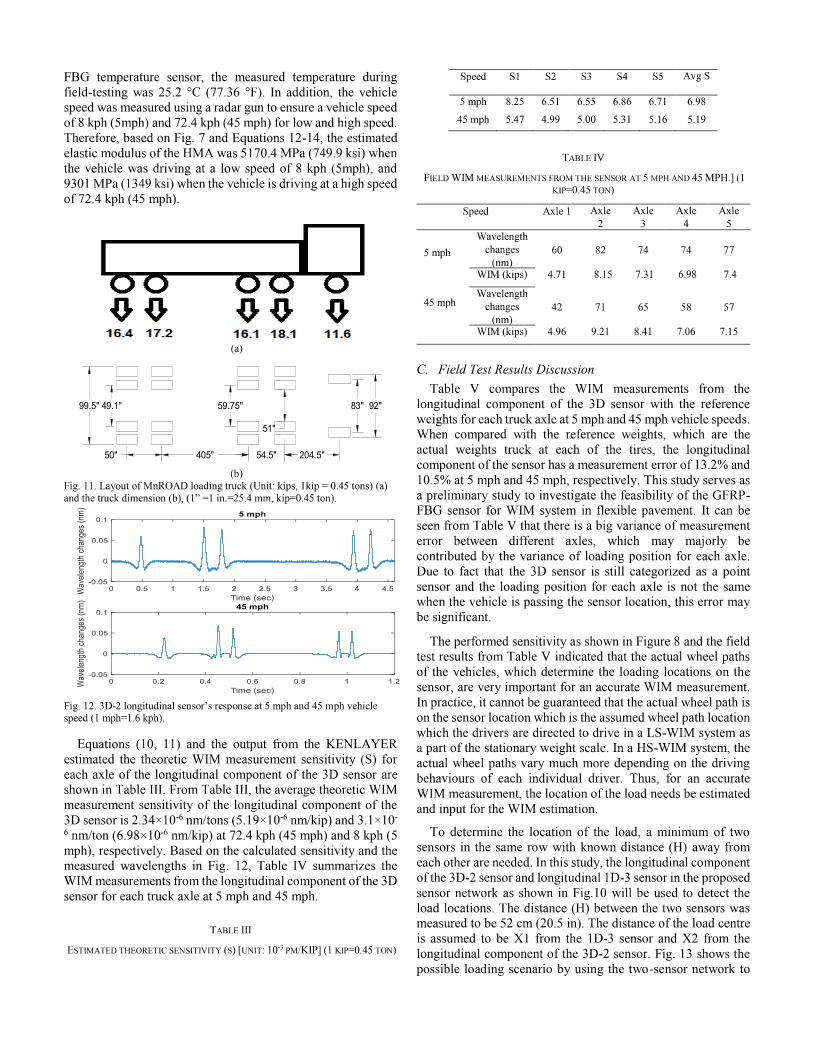
FBG temperature sensor, the measured temperature during field-testing was 25 .2 °C (77.36 °F). In addition, the vehicle speed was measured using a radar gun to ensure a vehicle speed of8 kph (5mph) and 72.4 kph (45 mph) for low and high speed. Therefore, based on Fig. 7 and Equations 12-14, the estimated elastic modulus of the HMA was 5170.4 MPa (749.9 ksi) when the vehicle was driving at a low speed of 8 kph (5mph), and 9301 MPa (1349 ksi) when the vehicle is driving at a high speed of72.4 kph (45 mph).

I 00 00

~ 0 I

00 00 0 1 6.4 1 7 .2 1 6.1 1 8.1 11 .6

(a)

GB CJ CJ CJ CJTT CJ T CJ I l__!g I

CJU CJ _l_CJ CJ CJ 9= - ~ +- +- - ~

(b) Fig. 11. Layout ofMnROAD loading truck (Unit: kips, !kip= 0.45 tons) (a) and the truck dimension (b ), ( =25.4 mm, kip=0.45 ton).

t ···: _r ;;Jt" : Ad ~ -0.05 ~--~--~--~--~---~-~ S: 0 0 .2 0.4 0.6 0 .8 1.2

Time (sec)

Fig. 12. 3D- ph vehicle speed (1 mph=l .6 kph).

Equations (10, 11) and the output from the KENLA YER estimated the theoretic WIM measurement sensitivity (S) for each axle of the longitudinal component of the 3D sensor are shown in Table III. From Table III, the average theoretic WIM measurement sensitivity of the longitudinal component of the 3D sensor is 2.34xI0-6 nm/tons (5 .19xI0-6 nm/kip) and 3.Ix10-6 nm/ton (6.98xI0-6 nm/kip) at 72.4 kph (45 mph) and 8 kph (5 mph), respectively. Based on the calculated sensitivity and the measured wavelengths in Fig. 12, Table IV summarizes the WIM measurements from the longitudinal component of the 3D sensor for each truck axle at 5 mph and 45 mph.

TABLE III

ESTIMATED THEORETIC SEN SITIVITY (S) [UNIT: 10·3 PM/KIP](! KIP=0.45 TON)

Speed SI S2 S3 S4 S5 AvgS

5mph 8.25 6.51 6.55 6.86 6.71 6.98

45mph 5.47 4.99 5.00 5.31 5.16 5.19

TABLE IV

FIELD WIM MEASUREMENTS FROM THE SEN SOR AT 5 MPH AND 45 MPH.] (1 KIP=0.45 TON)

Speed Axle I Axle Axle Axle Axle 2 3 4 5

Wavelength

5mph changes (nm}

60 82 74 74 77

WIM (kips) 4.71 8.15 731 6.98 7.4

45mph Wavelength

changes 42 71 65 58 57 (nm}

WIM (kips) 4 .96 9.21 8.41 7.06 7.15

C. Field Test Results Discussion

Table V compares the WIM measurements from the longitudinal component of the 3D sensor with the reference weights for each truck axle at 5 mph and 45 mph vehicle speeds. When compared with the reference weights, which are the actual weights truck at each of the tires, the longitudinal component of the sensor has a measurement error of 13 .2 % and 10.5% at 5 mph and 45 mph, respectively. This study serves as a preliminary study to investigate the feasibility of the GFRP­FBG sensor for WIM system in flexible pavement. It can be seen from Table V that there is a big variance of measurement error between different axles, which may majorly be contributed by the variance of loading position for each axle. Due to fact that the 3D sensor is still categorized as a point sensor and the loading position for each axle is not the same when the vehicle is passing the sensor location, this error may be significant.

The performed sensitivity as shown in Figure 8 and the field test results from Table V indicated that the actual wheel paths of the vehicles, which determine the loading locations on the sensor, are very important for an accurate WIM measurement. In practice, it cannot be guaranteed that the actual wheel path is on the sensor location which is the assumed wheel path location which the drivers are directed to drive in a LS-WIM system as a part of the stationary weight scale. In a HS-WIM system, the actual wheel paths vary much more depending on the driving behaviours of each individual driver. Thus, for an accurate WIM measurement, the location of the load needs be estimated and input for the WIM estimation.

To determine the location of the load, a minimum of two sensors in the same row with known distance (H) away from each other are needed. In this study, the longitudinal component of the 3D-2 sensor and longitudinal 1D-3 sensor in the proposed sensor network as shown in Fig. IO will be used to detect the load locations. The distance (H) between the two sensors was measured to be 52 cm (20.5 in). The distance of the load centre is assumed to be XI from the 1D-3 sensor and X2 from the longitudinal component of the 3D-2 sensor.

determine the location of the load at the time of weighing. Fig. 13 indicates that there are three loading scenarios including: Scenario 1) the load is in between of the two sensors, where X1+X2=H; Scenario 2) the load is on the right of the sensor 3D-2, where X2=X1-H; and Scenario 3) the load in on the left of the 1D-3 sensor, where X1=X2-H. Since the loading position is a two dimensions problem, the proposed methodology will work for scenario 1 where the condition X1+X2=H is stated.

l l e f=D = ´ ´ ´ ´ -

l l e f= D = ´ ´ ´ ´ -

where, λ and λ

weight, ε and εϕ

) is the strain sensitivity. Since the strains at the sensor’s location (ε and ε

single wheel, the first axle’s wheel will be used to validate the

pavement. Fig. 16 shows the simulated sensor’s response (S1 e load location (X) for the first axle’s right tire

sensor equals to 0.08 nm for the first axle’s tire. Following the

ε) within the sensor sensitivity range. (ε vs X)

Fig. 13. Possible loading scenarios for single wheel tire.

In order to investigate the ability of the system to determine the location of a moving load in between, distances Xl and X2

should be estimated for all scenarios from the actual sensor response. From Equation 11, the 1D-3 sensor response (S1) and the 3D-2 sensor longitudinal component response (S2) can be determined as follow:

p

2 p 2

(1 P.,)

(1 P.,) (15)

(16)

1 2 are the center wavelengths of 1D-3 and the longitudinal part of3D-2 sensor, respectively, Pis the measured

1 2 are the induced strain in the host material due to the load P at sensor S1 and sensor S2 location, respectively, is the strain transfer rate of the GFRP to host material, and ( 1-

1 2) are a function of the load location (Xl and X2) and the load P and it is hard to analyze the response of the flexible pavement theoretically. In this study, similar at in the sensitivity study, the KENLA YER software is used in this study to determine the strains at the sensor location with different loading locations.

TABLEV

COMPARISON OF THE WIM MEASUREMENTS WITH REFERENCES (1 KIP=0.45 TON, 1 MPH=l .6 KPH)

Measured Weight

Reference

5mph

45 mph

WIM (Kips)

5.8

4.71

4.37

Axle 1 Error (%)

18.7

14.32

Axle2 WIM (Kips) 9.05

8.15

8.82

Error (%)

9.9

1.9

Fig.14 shows the developed procedure used to calculate the actual distances Xl and X2 for a given load, pavement temperature, and vehicle speed with the measured strains. Estimating the pavement dynamic modulus, E*, is a significant input to construct KENLA YER model. For a given temperature and speed, the developed Master curve can be used to estimate E *. Then, the given load and estimated E * are used to construct KENLA YER model, which can be used to calculate the strain at any distance from the load and construct a strain as a function ofX (load location). The strain function can be used to estimate the sensor response (S1 and S2) using Equations (15 and 16). Then, the actual sensors response can be used to determine Xl andX2.

In order to validate the system to determine the load location, another field test was performed on May 2019 using the 5-axle semi-truck for three times on the three different locations as shown in Fig.13. The speed was recorded using the radar gun, which was 30 mph for all three runs. The pavement temperature was recorded using the FBG temperature compensation sensor, which is recorded to be 10.8 °C (51.4 °F). The first loading location was in the middle of the two sensors with Xl =H/2, the second loading location was on the 1D sensor with Xl=0, and the third loading location was on the 3D sensor with Xl =H. Fig. 15 shows the recorded sensor responses with the three different loading locations, respectively. Since the developed methodology can only determine the loading position for a

developed methodology.

Axle3 Axle4 WIM (Kips) 8.05

7.31

8.28

Error (%)

9.14

4.49

WIM (Kips)

8.6

6.98

6.94

Error (%)

18.82

17.8

Given temperature, and speed.

Estimate Dynamic modulus (E')

Construct KENLA YER model

Estimate strain (

Estimate S1 and S2 (Estimated S1 vs XI) and (Estimated S2 vs X2)

Solve for XI and X2 using actual S1 and S2

Fig. 14. Loading position estimation methodology.

Axle 5 WlM (Kips)

8.2

7.4

7.27

Error (%)

9.34

12.7

The recorded temperature and the speed were used to estimate the dynamic modulus of the pavement, which resulted in a dynamic modulus of 15,265 MPa (2,214.1 ksi) for the

and S2) with th of the truck. The first run of the vehicle has an actual sensor response for 1D-3 sensor equals to 0.055 nm and for 3D-2

procedure in Fig. 14 and the measured sensor response in Fig.

r’s response at 30 mph truck speed

and 1D sensor’s responses

The sensor’s WIM measurement sensitivity will decrease

rors’ effects

ACKNOWLEDGMENT

15, the value ofXl and X2 was determined to be 29.8 cm (11.74 in.) and 25.4 cm (10.01 in.), respectively. Both distances comply with Scenario 1 condition (Xl+X2=H±2.54 cm (1 in.)).

_/: t-----1 ~ ;J;A=~l 1

C -0 . 1 ~---~-------------0 1 2 3 4

! :: li---------;u a3 -0 . 1 ~---~-------------cu O 1 2 3 4

~::11-..•~ Ad -0 . 1 ~-~--~-~--~-~-----

1 1 .5 2 2 .5 3 3 .5 4 4 .5

Time (sec) Fig. 15. 3D-2 and ID senso (lmph=l.6kph) for three locations with Xl=H/2, Xl=0 and Xl=H from top to bottom.

0 .25 ,----~--~---~--~----,

0 .2

E ..s Q)

~ 0 .15 0 C. UJ

~ 0 0 .1 UJ <= Q)

en 0.05

5 10 15 20 25 Distance (in)

Fig. 16. Simulated sensor response changes with load locations (1 in=25.4 mm).

Table VI shows the corrected weights for the first axle of the 5-axle truck based on the estimated loading position. From Table VI, it is obvious that the weights corrected by the real­time estimated wheel path has a much accuracy with maximum error of 5.5%. The developed loading position correction methodology significantly reduces the inaccuracy of the measurements to allowable limit less than 10% and eliminate the error variances among the two sensors since the sensors have a big variance in error measurements.

TABLE VI FIELD WIM MEASUREMENTS BASED ON THE CALCULATED

LOADING POSITION AT 30 MPH (1 KIP=0.45 TON)

Reference weight (kips) 5.8

Wavelength (pm) changes (pm) 80 WIM (kips) 5.70 Error(%) 1.6

Wavelength (pm) changes (pm) 44 2

WIM (kips) 5.48

3

Error(%)

Wavelength (pm) (pm)

WlM (kips)

Error(%)

5.5

28

5.69

1.9

In addition, to test the repeatability of the sensors, both 3D (for more than 9 runs) at 30 mph

vehicle speed has been used assuming the first calculated weight is the reference weight. Both sensors have shown a repeatability of 98%.

VI. CONCLUSIONS AND FUTURE WORK

In this research, the authors developed a WlM system to investigate the feasibility of the 3D GFRP-FBG sensors for weight estimation of vehicle wheels in motion at low and high vehicle speed in challenging environment of the flexible pavement by conducting field validation testing under controlled condition (temperature, vehicle speed, and load location). The conclusions of this paper are: 1) The WIM system can survive the harsh process of

pavement construction. 2) The GFRP-FBG sensor is very sensitive to installation

depth and the best performance for WIM measurements is to install the sensor at the bottom of the pavement sections.

3) with the increase of the modulus of the embedded host materials.

4) All sensor components have maximum WIM sensitivity when applying a load directly over the sensor; the longitudinal component has the largest sensing radius for WlM measurement.

5) Field testing validated that the longitudinal component of the sensor has a measurement error of 13.2% and 10.5% at 5 mph and 45 mph vehicle speed, respectively.

6) The developed loading position correction methodology significantly reduces the inaccuracy of the measurements to less than 5.5%.

There are many error sources affecting the accuracy of the measurements including seasonal temperature variance, vehicle speed, vehicle weight, and estimating the modulus of elasticity through the master curve, etc. All these er will be further studied and their contributing factors on measurement accuracy will be investigated and reported in our future study.

This study was partially supported by the U.S. Department of Transportation under the agreement No.69A35517477108 through Mountain-Plains Consortium Project No. MPC-547, a NSF award under Agreement No.1750316, and NSF ND EPSCoR DDA Program. The findings and opinions expressed in this article are those of the authors only and do not necessarily reflect the views of the sponsors.

REFERENCES

[1] American Association of State Highway and Transportation Officials, AASHTO Guide for Design

Y. Jiang, S. Li, T. Nantung, and H. Chen, “Analysis

empirical pavement design guide,”

P. Szary and A. Maher, “Implmotion (wim) systems,” 2009.B. LE Jinwoo and C. Hanseon, “Commercial Vehicle Preclearance Program: Motor Carriers’ Perceived

Implementation,” in

O. Norman and R. Hopkins, “Weighing vehicles in motion,” R. Bushman and A. J. Pratt, “Weigh in Motion

Economics and Performance,” in

Gajda, “Thermal Property Analysis of

Motion System,” Sensors, vol.16, no.12, 2016.[8] J. Gajda, P. Burnos, and R. Sroka, “Weigh

systems for direct enforcement in Poland,” in

–

L. Zhang, C. Haas, and S. L. Tighe, “Evaluating

Data Collection,” –

“Fibre Bragg gratings in structural health monitoringPresent status and applications,”

–R. B. Malla, A. Sen, and N. W. Garrick, “A

Vehicles on Highways,” –

S. Oh and J. Sim, “Interface debonding failure in beams strengthened with externally bonded GFRP,”

–

Huang, and O. Jinping, “Optical fiber Bragg grating

study in highway pavement,” –

“Glass fiber

overlay monitoring,” –

Tarawneh and Y. Huang, “Glass fiber

measurements,”

, “Photosensitivity in optical fiber

fabrication,” –

Transportation Officials (AASHTO), “Standard

Hot Mix Asphalt (HMA),” 2011.

Strommen, “Sampling op

based sensors,”

Tarawneh and Y. Huang, “In

estimation,” in

“Vehicle Classification System Using Inrating Sensors,”

(M’91 SM’02)

[2]

of Pavement Structures, 1993. Washington,D.C: American Association of State Highway and Transportation Officials, 1993.

and determination of axle load spectra and traffic input for the mechanistic-

Aug. 2016. [17] K. 0 . Hill, Y. Fujii, D. C. Johnson, and B. S.

Kawasaki waveguides: Application to reflection filter

Appl. Phys. Lett., vol. 32, no. 10, pp. 647 649, 1978.

2008. [18] Y. Huang, Pavement analysis and design, 2nd ed. Upper Saddle River,NJ: Pearson Prentice Hall, 2004. American Association of State Highway and

[3]

[4]

[5]

[6]

ementation of weigh-in-

Impacts and Attitudes towards Potential the Eastern Asia Society for

Transportation Studies, 2013 .

Highw. Res. Board Bull., vol. 50, 1952.

Technology­NATMEC, 1998, p. 7.

[7] P .Burnos and J. Axle Load Sensors for Weighing Vehicles in Weigh­m-

-in-Motion

ICWIM7: 7 International Conference on Weigh-in­Motion & PIARC workshop, 2016, pp. 302 311.

[9] S. H. Vaziri, "Investigation of Environmental Impacts on Piezoelectric Weigh-In-Motion Sensing System," Ph.D dissertation, Civil Eng., University of Waterloo., Ontario, Canada 2011.

[l O] Weigh-In-Motion Sensing Technology for Traffic

Transportation Association of Canada, Saskatoon, Saskatchewan, pp. 1 17, 2007.

[11] M. Majumder, T. K. Gangopadhyay, AK. Chakraborty, K. Dasgupta, and D. K. Bhattacharya,

Sensors Actuators, A Phys., vol. 147, no. 1, pp. 150 164, 2008.

[ 12] Special Fiber Optic Sensor for Measuring Wheel Loads of

Sensors, vol. 8,no.4,pp. 2551 2568, Apr. 2008.

[13] H.-

Compos. Interfaces, vol. 11, no. 1, pp. 25 42, 2004. [14] Z. Zhou, W. Liu, Y. Huang, H. Wang, H. Jianping, M.

sensor assembly for 3D strain monitoring and its case Mech. Syst. Signal

Process., vol. 28, pp. 36 49, 2012. [15] Z. Zhang, Y. Huang, L. Palek, and R. Strommen,

-reinforced polymer-packaged fiber Bragg grating sensors for ultra-thin unbonded concrete

Struct. Heal. Monit., vol. 14, no. 1, pp. 110 123, 2015.

[16] M. Al-reinforced polymer packaged fiber Bragg grating sensors for low-speed weigh-in-motion

Opt. Eng., vol. 55, no. 8, p. 086107,

[19]

Method of Test for Determining Dynamic Modulus of

[20] Z. Zhang, Y. Huang, R. Bridgelall, L. Palek, and R. timization for high-speed

weigh-in-motion measurements using in-pavement strain- Meas. Sci. Technol., vol. 26, no. 6,p.065003,2015.

[21] M. Al- -pavement fiber Bragg grating sensor for vehicle speed and wheelbase

Sensors and Smart Structures Technologies for Civil, Mechanical, and Aerospace Systems 2018, 2018, vol. 10598, p. 105982A.

[22] M. Al-Tarawneh, Y. Huang, P. Lu, and D. Tolliver, -pavement

Fiber Bragg G IEEE Sens. J., 2018.

Dr. Mu'ath Al-Tarawneh received Ph.D. degree in civil engineering at North Dakota State University (NDSU), Fargo, USA, in 2019. He completed his M.S. degree at NDSU, Fargo, in 2016. His research interest is in intelligent transportation systems.

Dr. Ying Huang is an associate professor in the department of civil and environmental engineering at NDSU. She received her Ph.D. degree from the Missouri University of Science and Technology in 2012. Her research interests include intelligent transportation system, corrosion mitigation and assessment, smart

structures and structural health monitoring.

Dr. Pan Lu received her Ph.D. degree in transportation and logistics at NDSU in 2009. In 2010, Dr. Lu became a research analyst at the Upper Great Plains Transportation Institute (UGPTI) at NDSU. From 2012 to 2016, Pan has served as associate research fellow and assistant

professor at UGPTI. Beginning in 2017, Dr. Lu is an associate professor in the College of Business at NDSU.

Dr. Raj Bridgelall received the Ph.D. degree in transportation and logistics from NDSU, Fargo, in 2015. He served as the RFID Chief Technologist at Motorola until 2004, as Vice President of Research & Development at Alien

Technology until 2006, and as Chief Technical Officer at Axcess International until 2010. He is presently Program Director of the SMARTSesM Intelligent Transportation Systems Center at NDSU.