pre-runtime scheduling of an avionics system -...

IT 16 043

Examensarbete 30 hpJune 2016

Pre-Runtime Scheduling of an Avionics System

Max Block

Institutionen för informationsteknologiDepartment of Information Technology

Teknisk- naturvetenskaplig fakultet UTH-enheten Besöksadress: Ångströmlaboratoriet Lägerhyddsvägen 1 Hus 4, Plan 0 Postadress: Box 536 751 21 Uppsala Telefon: 018 – 471 30 03 Telefax: 018 – 471 30 00 Hemsida: http://www.teknat.uu.se/student

Abstract

Pre-Runtime Scheduling of an Avionics System

Max Block

This master’s thesis addresses a scheduling problem arising when designing avionics– the electronic systems used on aircraft. Currently, the problem is commonlysolved using mixed integer programming (MIP). We prove the scheduling problemat-hand, which is similar to the well-studied cyclic job shop scheduling problem,is NP-hard. Furthermore, we propose an approach using constraint programming(CP) – a programming paradigm where entities called constraints define the relationsbetween variables. Constraints do not specify a step or sequence of steps toexecute, but rather the necessary properties of a solution. The CP approachimplementedin the high-quality free OscaR CP solver manages around 1500 tasks in totalover 10 processors within a 10 minute timeout, which is good enough for CP to beinvestigated further as a possible paradigm for solving the considered schedulingproblem. We also compare Gurobi Optimizer, a high-quality commercial MIP solver,to Gecode, another high-quality free CP solver, when run on a model for the problemdescribed in the MiniZinc modelling language.

Tryckt av: Reprocentralen ITCIT 16 043Examinator: Edith NgaiÄmnesgranskare: Pierre FlenerHandledare: Elina Rönnberg

Acknowledgements

I would like to thank Isak Bohman for letting me use your scheduling probleminstance generator when developing a generator for instances of this thesis’ problem.

Thank you, Jean-Noel Monette, for giving me a solid foundation for constraintmodelling both in MiniZinc and in general. Thank you, also, for taking the time toanswer all my questions.

And last, but certainly not least, I would like to thank Pierre Flener. Thank youfor kindling my interest in CP, for helping me structure my thesis work, and fortirelessly and thoroughly helping me fine-tune my report.

5

Contents1 Introduction 9

1.1 Setting . . . . . . . . . . . . . . . . . . . . . . . . . . . . . . . . . . . . . . . . . . 91.2 Questions . . . . . . . . . . . . . . . . . . . . . . . . . . . . . . . . . . . . . . . . . 91.3 Scope . . . . . . . . . . . . . . . . . . . . . . . . . . . . . . . . . . . . . . . . . . . 9

2 Background 102.1 Real-Time Scheduling . . . . . . . . . . . . . . . . . . . . . . . . . . . . . . . . . . 10

2.1.1 The basics . . . . . . . . . . . . . . . . . . . . . . . . . . . . . . . . . . . . 102.1.2 The precedence relation . . . . . . . . . . . . . . . . . . . . . . . . . . . . 112.1.3 Hard and soft real-time systems . . . . . . . . . . . . . . . . . . . . . . . . 112.1.4 On-line vs. pre-runtime scheduling . . . . . . . . . . . . . . . . . . . . . . 11

2.2 MiniZinc . . . . . . . . . . . . . . . . . . . . . . . . . . . . . . . . . . . . . . . . . 122.3 OscaR . . . . . . . . . . . . . . . . . . . . . . . . . . . . . . . . . . . . . . . . . . . 122.4 Gantt charts . . . . . . . . . . . . . . . . . . . . . . . . . . . . . . . . . . . . . . . 132.5 Random Forests . . . . . . . . . . . . . . . . . . . . . . . . . . . . . . . . . . . . . 13

2.5.1 Decision Trees . . . . . . . . . . . . . . . . . . . . . . . . . . . . . . . . . . 132.5.2 Random Forests . . . . . . . . . . . . . . . . . . . . . . . . . . . . . . . . . 14

3 Job Shop Scheduling 143.1 Problem Statement . . . . . . . . . . . . . . . . . . . . . . . . . . . . . . . . . . . 143.2 Cyclic Job Shop Scheduling . . . . . . . . . . . . . . . . . . . . . . . . . . . . . . . 15

4 Constraint Programming 164.1 Constraint Satisfaction Problems . . . . . . . . . . . . . . . . . . . . . . . . . . . 164.2 Propagation . . . . . . . . . . . . . . . . . . . . . . . . . . . . . . . . . . . . . . . 17

4.2.1 Propagators . . . . . . . . . . . . . . . . . . . . . . . . . . . . . . . . . . . 174.2.2 Consistency . . . . . . . . . . . . . . . . . . . . . . . . . . . . . . . . . . . 174.2.3 Propagation step . . . . . . . . . . . . . . . . . . . . . . . . . . . . . . . . 18

4.3 Global Constraints . . . . . . . . . . . . . . . . . . . . . . . . . . . . . . . . . . . . 184.4 Search . . . . . . . . . . . . . . . . . . . . . . . . . . . . . . . . . . . . . . . . . . . 19

4.4.1 Branching . . . . . . . . . . . . . . . . . . . . . . . . . . . . . . . . . . . . 194.4.2 Exploration . . . . . . . . . . . . . . . . . . . . . . . . . . . . . . . . . . . 21

4.5 Constrained Optimisation Problems . . . . . . . . . . . . . . . . . . . . . . . . . 214.6 Implied Constraints . . . . . . . . . . . . . . . . . . . . . . . . . . . . . . . . . . . 214.7 Symmetry Exploitation . . . . . . . . . . . . . . . . . . . . . . . . . . . . . . . . . 214.8 Reification . . . . . . . . . . . . . . . . . . . . . . . . . . . . . . . . . . . . . . . . 22

5 Scheduling of an Avionic System 225.1 Problem Statement . . . . . . . . . . . . . . . . . . . . . . . . . . . . . . . . . . . 225.2 Problem Complexity . . . . . . . . . . . . . . . . . . . . . . . . . . . . . . . . . . 235.3 Characteristics of Instances in Avionics . . . . . . . . . . . . . . . . . . . . . . . . 24

6 Constraint Model 246.1 Instance Data and Derived Constants . . . . . . . . . . . . . . . . . . . . . . . . . 246.2 Decision Variables . . . . . . . . . . . . . . . . . . . . . . . . . . . . . . . . . . . . 246.3 No Task is Crossing the Cycle Boundary . . . . . . . . . . . . . . . . . . . . . . . 256.4 Tasks on the Same Timeline May Not Overlap . . . . . . . . . . . . . . . . . . . . 256.5 Respecting Precedences . . . . . . . . . . . . . . . . . . . . . . . . . . . . . . . . . 26

7

6.6 A Chain Must Completely Finish Before Its Next Iteration . . . . . . . . . . . . . 27

7 Test Instances 287.1 Algorithm Idea . . . . . . . . . . . . . . . . . . . . . . . . . . . . . . . . . . . . . . 297.2 Tasks . . . . . . . . . . . . . . . . . . . . . . . . . . . . . . . . . . . . . . . . . . . 297.3 Chains . . . . . . . . . . . . . . . . . . . . . . . . . . . . . . . . . . . . . . . . . . 317.4 Input Parameters . . . . . . . . . . . . . . . . . . . . . . . . . . . . . . . . . . . . 31

8 Search 338.1 The First-Fail/Best-First Principle . . . . . . . . . . . . . . . . . . . . . . . . . . . 338.2 Min/Min Scheme . . . . . . . . . . . . . . . . . . . . . . . . . . . . . . . . . . . . 338.3 SetTimes Branching . . . . . . . . . . . . . . . . . . . . . . . . . . . . . . . . . . . 348.4 Conflict Ordering Search . . . . . . . . . . . . . . . . . . . . . . . . . . . . . . . . 34

8.4.1 Last-Conflict Based Reasoning . . . . . . . . . . . . . . . . . . . . . . . . . 348.4.2 Conflict Ordering Search . . . . . . . . . . . . . . . . . . . . . . . . . . . . 34

8.5 Accumulated Failure Count Based Variable Selection . . . . . . . . . . . . . . . . 35

9 Experimentation 359.1 Instance Selection . . . . . . . . . . . . . . . . . . . . . . . . . . . . . . . . . . . . 36

9.1.1 Machine Characteristics . . . . . . . . . . . . . . . . . . . . . . . . . . . . 369.1.2 Selecting Test Instances . . . . . . . . . . . . . . . . . . . . . . . . . . . . . 369.1.3 Selected Test Instances/Test Method . . . . . . . . . . . . . . . . . . . . . 37

9.2 OscaR Experimentation . . . . . . . . . . . . . . . . . . . . . . . . . . . . . . . . . 389.2.1 Machine Characteristics . . . . . . . . . . . . . . . . . . . . . . . . . . . . 389.2.2 Results . . . . . . . . . . . . . . . . . . . . . . . . . . . . . . . . . . . . . . 389.2.3 OscaR Model Evaluation . . . . . . . . . . . . . . . . . . . . . . . . . . . . 41

9.3 Solver Technology Comparison . . . . . . . . . . . . . . . . . . . . . . . . . . . . 419.3.1 Machine Characteristics . . . . . . . . . . . . . . . . . . . . . . . . . . . . 429.3.2 Experimental Setup . . . . . . . . . . . . . . . . . . . . . . . . . . . . . . . 429.3.3 Results . . . . . . . . . . . . . . . . . . . . . . . . . . . . . . . . . . . . . . 429.3.4 Conclusion . . . . . . . . . . . . . . . . . . . . . . . . . . . . . . . . . . . . 44

10 Conclusion 45

11 Future Work 4511.1 Search Based on Instance Structures . . . . . . . . . . . . . . . . . . . . . . . . . . 4511.2 Implied Constraints and Symmetry Breaking . . . . . . . . . . . . . . . . . . . . 4511.3 Optimisation . . . . . . . . . . . . . . . . . . . . . . . . . . . . . . . . . . . . . . . 4611.4 Limited Discrepancy Search . . . . . . . . . . . . . . . . . . . . . . . . . . . . . . 46

References 47

8

1 Introduction

1.1 SettingAmodern aeroplane hosts lots of advanced electronics; electronics in an aircraft setting is calledavionics. Avionic systems include communications, information-gathering sensors, processingunits refining the gathered information, equipment presenting the refined data to the pilot, andthe hundreds of systems that are fitted to an aircraft to perform individual functions. Thesecan as simple as an external flashing light, as complicated as the targeting system of a militaryaircraft, or anything in between.

Some units update the state of the aircraft repeatedly during operation, giving rise to acomplex flow of data between different units and thus putting requirements on the order ofthe activities’ executions. Furthermore, for an avionic system it is not sufficient that the logicalresult of a computation is correct; it is crucial that the result is produced at the correct timeand missing deadlines could lead to devastating events. In other words, avionic systems areexamples of hard real-time systems, see Section 2. The problem is similar to that of the Cyclic JobShop Problem defined in Section 3.

During the last two decades or so, a large part of the avionics industry has switched architec-ture paradigm from using federated systems, where each subsystem has its own computers per-forming its own functions, to using an integrated architecture called integrated modular avionics(IMA). IMA is a hard real-time multiprocessor system where applications share hardware re-sources.

The idea was to make more efficient use of a smaller amount of avionics, and the IMA ap-proach can cut off as much as half of the number of processors, as is the case for the AirbusA380 suite. Such an architecture necessitates strict requirements on the spatial and temporalpartitioning of the system to achieve fault containment, and a common standard for this parti-tioning is ARINC 653 [25, 29].

Typically, the IMA architecture gives rise to multiprocessor scheduling problems that be-come computationally demanding for large-scale instances. The introductory parts of the PhDthesis [1] provide an extensive introduction to the area of scheduling avionic systems. Findingan efficient solution method to such problems is necessary for being able to use IMA.

1.2 QuestionsThis master thesis addresses a sub-problem arising in the scheduling of an avionic system,defined in Section 5, and it is part of a research project collaboration between Linkoping Uni-versity and Saab. The goal is to solve the problem using a constraint programming approachimplemented as a scheduling tool. Constraint programming is defined in Section 4, and theimplementation is described in Sections 6 and 8. The purpose of the thesis is to evaluate theperformance of this scheduling tool and determine if the approach is appropriate for the prob-lem at hand. A description of the experimental process is found in Section 9, the results inSection 9.2, and the conclusion in Section 10. In Section 11, we list some possible future exten-sions to the scheduling tool.

1.3 ScopeScheduling of real-time systems can refer to either on-line scheduling, where scheduling de-cisions are made during runtime, or pre-runtime scheduling, where the schedule is decided atcompile time. This project will consider pre-runtime scheduling, and all activities are repeated

9

within a certain time frame, making the schedule cyclically repeated with requirements span-ning between the end and beginning of the schedule.

The focus of this thesis is to find a constraint programming based solution capable of findingsolutions to instances of the scheduling problem within reasonable time and computationalresources for instances of real-life size.

Due to confidentiality reasons the evaluation instances are not real avionic data, but rathersharing characteristics with real instances with respect to task durations, dependency metadata, etc. Part of the thesis is designing a tool for generating test instances. This is furtherdescribed in Section 7.

2 BackgroundThe following material contains the necessary terminology as well as some background to theproblem stated in Section 5.

2.1 Real-Time SchedulingA more thorough description of real-time scheduling and real-time systems is given by Kopetzin [15].

2.1.1 The basics

In scheduling problems, one is considering a finite set of units of execution called tasks respectinga finite set of constraints. In this thesis, a task τ is a triple �EST,LCT,δ� which are to be inter-preted as an earliest starting time, a latest completion time, and a duration, respectively. The LCTmay also be called the deadline. The tasks are to be placed in a schedule such that all tasks arescheduled, all tasks start after their EST, end before their LCT, and execute for their respectiveduration.

Tasks share a set of resources, corresponding to e.g. CPUs or places in memory, and schedul-ing is assigning a starting time and a resource to each task such that the start time is at leastthe EST and the start time plus the duration is at most the LCT. The resources usually havean upper bound on concurrent usage, such as a single-core processor, which only one task at atime may be scheduled to use. Furthermore, tasks are usually related by precedence, restrictingthe order in which tasks may be executed. A schedule satisfying all scheduling constraints iscalled feasible.

In some settings, there is an evaluation function taking a feasible schedule as input, mappingit to a real number. Then the solutions can be ordered and an optimal schedule is one eitherminimising or maximising the evaluation function. An optimal schedule could, e.g., be the oneminimising the end time of the last task.

Sometimes, a task is also associated with a value describing how much of a resource is con-sumed during execution. However, in this thesis, all tasks are using exactly one resource uniteach, making such values superfluous.

A cyclic scheduling problem is a scheduling problem where all tasks must occur an indefinitenumber of times. Cyclic scheduling problems exist in many domains including:

• Parallel computing, where loop scheduling problems occur when designing optimisingcompilers for parallel architecture computers [11].

• Automated manufacturing systems, where many activities usually correspond to cyclicoperations [2]. For instance, tasks executed by industrial robots on mass production line

10

machines are repeated cyclically. Also, the maintenance tasks executed by technicians onthese robots occur cyclically during the production process after a fixed time of machin-ing.

• Many common human activities can be viewed as cyclic activities. For instance, timetabling activities in a school typically consist of finding a week-long cycle to be repeatedover a certain duration such as the whole school year or semester.

2.1.2 The precedence relation

Tasks may be subject to precedence constraints. Precedence is a binary relation over tasks where(τ1,τ2) is in the relation if and only if τ1 has finished executing before τ2 starts to execute. Thatis, the start time of τ1 plus its duration is at most the start time of τ2. The precedence relationin an instance can be viewed as a directed graph.

We denote that the dependency (τ1,τ2) is an element in this relation by τ1 ≺ τ2. Each de-pendency is here associated with a gap range [γmin,γmax]. At least γmin time units must passbetween the end of execution of τ1 and the beginning of τ2, and the same span may be at mostγmax units long.

2.1.3 Hard and soft real-time systems

Real-time systems are often divided into three classes: hard, firm, and soft. In hard real-timesystems it is absolutely crucial deadlines are not missed, and failing to meet a deadline leads tosystem failure and often severe consequences [15]. For example, systems for medical purposesmay be hard, if missing deadlines may lead to lives lost.

In firm and soft real-time systems, the system is not considered to have failed even aftermissing a few deadlines. A system where results have no practical use after a missed deadlineis often called firm, whether late results in soft systems may still have some use. A systemforecasting weather is firm since a missed deadline is (usually) not disastrous but the computedresult is not worth anything when the time of the forecast has passed.

2.1.4 On-line vs. pre-runtime scheduling

Scheduling can be either on-line or pre-runtime. On-line scheduling is done during operationand consists of following a set of pre-defined rules for determining which task a processingunit should work on. On-line scheduling is usually very memory-efficient, and will often leadto a high throughput of tasks due to its flexibility. In some cases, however, on-line schedulingwill lead to tasks missing their deadlines, especially in non pre-emptive systems, where anexecuting task may not be stopped before its completion. For example, assume a processingunit has just started on a task taking a large amount of time to compute when another task withan early deadline is deployed. It may then be impossible to finish the second task before itsdeadline, making the schedule infeasible.

Pre-runtime scheduling, on the other hand, is done before operation and consists of con-structing a schedule that is then followed during runtime. Such schedules can be extremelylarge and thus memory-consuming. On the other hand, finding a feasible, or even optimal,schedule guarantees no task will ever miss their respective deadline, making them suitable forhard real-time systems.

On-line scheduling algorithms usually are based on making locally good decisions andtherefore are low in time complexity. E.g., earliest deadline first (EDF) where, whenever ascheduling event occurs such as a task finishing, the task closest to its deadline is the next to

11

be scheduled for execution. Finding the task with the earliest deadline is linear, and thereforepolynomial, in the number of tasks to be scheduled.

Pre-runtime scheduling, on the other hand, is a harder problem to solve if feasible or evenoptimal schedules are required. Cyclic scheduling problems can be roughly classified intotwo main categories: problems without resource constraints and problems with resource con-straints. Among the first category are the following two problems:

• The basic cyclic scheduling problem (BCS) consists of assigning starting times from R toa finite set of tasks in a schedule, where no resource constraints are considered. Eachtask is to be scheduled � times. The aim is to minimise the total runtime divided by thenumber � as � goes to infinity. The tasks are subject to uniform constraints, which areconstraints (i, j,k) on tasks τi ,τj stating that τi must have executed k times more than τj .These constraints are called uniform since k is constant. The problem is stated by Hanenand Munier in [11], and proven to be solvable in O(n3 · logn) time where n is the numberof tasks.

• In [21], Munier extends BCS to the basic cyclic scheduling problem with linear precedenceconstraints (BCSL) where k in BCS is no longer constant, but a linear polynomial k(�).Naturally, the polynomial k(�) is positive on N.

The second category, having resource constraints constraining the number of concurrent tasks,are:

• The hoist scheduling problem (HSP) can be found in the electronics industry, where prin-ted circuit boards must undergo a sequence of chemical and electro-plating operations insuccessive tanks, corresponding to resources. There are robots or hoists transporting theparts that must avoid collisions on a common track. An infinite number of parts must beprocessed, and the objective is to minimise the average cycle time in the long run. For onerobot executing one job consisting of a set of tasks, the problem is (strongly) NP-hard [2].

• The cyclic job shop problem, discussed in Section 3.2.

2.2 MiniZinc

MiniZinc [20] is a constraint-based modelling language for constraint problems where modelsare usually easy to read and can be used as input for any back-end from a range of differenttechniques. There are, among others, back-ends using constraint programming, Section 4, orSAT solving, a field arising from trying to find a truth assignment satisfying a given Booleanformula. An example model can be seen in Figure 1.

2.3 OscaR

OscaR [22] is a Scala toolkit for solving Operational Research (OR) problems, and the abbrevi-ation stands for “Scala in OR”. The techniques currently available in OscaR are:

• Constraint programming (CP) (module based on the former Scampi).

• Constraint-based local search (module based on the former Asteroid).

• Linear programming.

• Discrete event simulation.

12

1: array[1..9, 1..9] of var 1..9: puzzle;2:3: % All different in rows4: constraint forall (i in 1..9) (5: alldifferent( [ puzzle[i,j] | j in 1..9 ]) );6:7: % All different in columns.8: constraint forall (j in 1..9) (9: alldifferent( [ puzzle[i,j] | i in 1..9 ]) );

10:11: % All different in sub-squares:12: constraint13: forall (a, o in 1..3)(14: alldifferent( [ puzzle[(a-1) *S + a1, (o-1)*S + o1] |15: a1, o1 in 1..3 ] ) );16:17: solve satisfy;

Figure 1: A constraint model of the Sudoku problem, written in the MiniZinc modelling lan-guage. Adapted from [19].

• Derivative free optimisation.

• Visualisation.

This thesis will only use the CP module of OscaR.

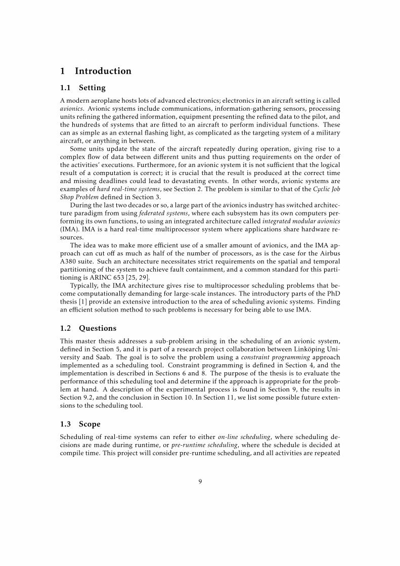
2.4 Gantt chartsA Gantt chart is a type of bar chart illustrating a project schedule. It is named after HenryGantt, an American mechanical engineer/management consultant, who developed the chartin the 1910s. However, it was independently invented by the Polish economist, engineer andmanagement researcher Karol Adamiecki in 1896.

Gantt charts are very useful for illustrating schedules such as those discussed in this report.Figure 2 depicts a Gantt chart representing a system for some timeframe. Each box correspondsto the execution of a task and each arrow to a dependency. Sometimes a row will represent asingle task for visibility reasons, as in Figure 3. Such cases are identified by the row labelling,using τ, or announcement in the text. Mostly a row will represent resources usable by at mostone task at a time (called unary).

2.5 Random ForestsWe discuss decision trees, a machine learning method for classification or regression, as well asthe extended method using a forest of decision trees.

2.5.1 Decision Trees

Decision tree learning uses a decision tree as predictive model, mapping variable observationsto conclusions about the target value. An example based on survival data of the Titanic is seenin Figure 4. Beginning at the root, we predict whether a person survives or not by progressing

13

p1

p2

p3

p4

Figure 2: Example Gantt chart.

τ1

τ2

τ3

Figure 3: Three tasks τ1,2,3 on separate rows.

downwards using the labelled branches. A male aged 9 would go left twice from the root andend in a red leaf representing likely death, whereas a female would go right once into a greenleaf representing likely survival. This is an example of classification, where the outcome is eithersurvival or death. Decision trees can also be used for regression, where the predicted outcomeis a real number, for example representing the predicted price of a consumer good.

Algorithms for constructing decision trees usually work top-down, choosing the variablethat best splits the training data, see [27]. Therefore, decision trees can be used for evaluatingthe importance of the different observed variables.

2.5.2 Random Forests

Random forests [14], or random decision forests, operate by constructing a multitude of decisiontrees at training time. Each tree is given a subset of the input data when training, and the res-ulting random forest model outputs the mean prediction of all trees in the forest for regressionmodels. Random forests correct for the individual decision trees’ habit of overfitting to theirtraining set, see [13].

3 Job Shop SchedulingWe define the job shop scheduling problem and extend it to the cyclic job shop schedulingproblem.

3.1 Problem StatementThe job shop scheduling problem (abbreviated JSP) is a problem where a number of tasksτ1,τ2, . . . ,τk are to be scheduled over a set of m distinct resources, e.g. processors.

14

Age ≤ 9.5

sib+ sp ≤ 2.5 sib+ sp > 2.5

Age > 9.5

Male Female

Figure 4: A decision tree showing a prediction of the survival of passengers on the Titanic basedon passenger observations. sib+ sp is the sum of siblings and spouses to the evaluated personaboard the ship. Red leaves indicate predicted death and green survival.

Each task τ has an earliest start time (EST), a latest completion time (LCT), and a durationδ. Furthermore, τ is associated with a resource rτ . While a task is using a resource, no othertask may use the same resource. Such a resource with capacity one is called unary. Pre-emptionis not allowed, meaning that a task that has started to execute must execute in its entirety.

Lastly, there is a set of precedence constraints of the form τi ≺ τj specifying that the task τimust be completed before τj can begin. Each precedence constraint is associated with a range[γmin,γmax] specifying that the time between the end of τi and the beginning of τj is within thisrange.

The problem may either be of schedule optimisation or of determining feasibility. In thefirst case, we aim for a solution having minimal makespan, which is the maximum completiontime of all tasks, or having maximal throughput, which is the number of completed tasks withinsome time frame, or some other optimisation metric. If determining feasibility, we aim to finda schedule where the makespan is at most some upper limit or prove no such schedule exists.More on the topic of the job shop scheduling problem can be found in [2, 3].

3.2 Cyclic Job Shop SchedulingIn the cyclic job shop problem (CJSP), we assume that the set of tasks is a template which wewish to repeat indefinitely. For example, the tasks may represent steps towards building awidget in a factory. Some parts usually need to be made in a particular order, so some tasksare subject to precedence constraints. In the CJSP, the construction of a single widget may spanover more than one cycle.

In a typical optimisation CJSP, we will want to overlap the construction of more than onewidget to make efficient use of the resources. In [10], it is shown that a non-cyclic schedulefor some given task set may outperform any cyclic schedule with respect to average makespan,i.e., the average cycle time when the number of instances of the task set goes to infinity. Thereare advantages to using cyclic schedules, however. First, cyclic schedules are much easier toimplement; we only need to communicate a short sequence of actions. Second, the cost ofcomputing optimal non-cyclic schedules grows exponentially with the number of widgets [3].

However, for the problem discussed in this thesis, instances of the same type of widget maynot be made in parallel. In addition, the same instance of a task is not allowed to execute overmore than one cycle. Furthermore, the aim will only be to find a feasible schedule rather thanfinding an, in some sense, optimal schedule.

More on the subject of the cyclic job shop problem as well as a formal definition can befound in [2, 3, 10].

15

4 Constraint ProgrammingConstraint programming (CP) is a programming paradigm wherein relations between variablesare stated in the form of constraints. A constraint does not specify how to find a solution,but rather a property of any solution to a given problem, making CP a form of declarativeprogramming.

In a constraint programming solver, propagators are posted with the sole responsibility ofmaking sure their respective constraints are not violated. The efficiency of a CP toolkit is highlycorrelated to how well its propagators are implemented.

Even though the terminology of CP may not be familiar, the basic concepts should be famil-iar to anyone who has tried to solve a Sudoku puzzle. Sudoku is a number puzzle in the formof a 9× 9 grid, divided into nine pairwise disjoint 3× 3 boxes. A Sudoku starts with some cellsprefilled with numbers, called clues. The puzzle is solved when each cell in the grid is filledwith a whole number in 1,2, . . . ,9, satisfying three rules:

1. The numbers in each row must be different from each other.

2. The numbers in each column must be different from each other.

3. The numbers in each 3× 3 box must be different from each other.

A Sudoku is an example of a constraint satisfaction problem (CSP) defined in Section 4.1. Sec-tion 4.5 will extend CSPs with an objective function in order to find a best solution to a givenproblem. Sections 4.2, 4.3, and 4.4 will further describe the methods of CP.

4.1 Constraint Satisfaction ProblemsA constraint satisfaction problem (CSP) is a triple �V ,D,C� consisting of a finite set V of decisionvariables, a domain function D defined on the variables vi in V mapping a variable to a set,and a finite set of constraints C. The store is the current collection of domains. The CSP issolvedwhen all decision variables in V have been assigned a single value within their respectivedomains such that all constraints are satisfied.

A store is said to be (strictly) stronger than another store if the (non-empty) store has at leastone domain being a proper subset of its counterpart in the weaker store. The strongest possiblestore is when all domains are singleton sets, and such stores correspond to a solution to the CSP.

In the case of Sudokus, each cell corresponds to a variable and each variable has the domain{1,2, . . . ,9}. Each of the three rules in the previous section applies to nine groups of nine cellseach, so in total the rules can be expressed using 27 constraints, each on nine variables.

Solving a CSP using a constraint programming solver is an iterative process alternatingbetween two states; propagation and search. During propagation, values are removed from thedomains until no more values can be removed by the propagators. During search, the solverdivides the search space into mutually exclusive alternatives, thereby creating a search tree. Inother words, if the solver branches on a variable, the intersection of the domains of that variablein any two branches is empty and the union of the domains in all branches is the domain beforebranching. Branching can make other decisions than variable assignments, e.g. the order oftasks in a schedule, as seen in Section 8.3. A partial assignment is any node different from theroot. There, the branching heuristics will have made a decision not necessarily logically impliedby the existing constraints.

For example, in one branch the solver may try to place the number 4 in a given cell in aSudoku, and exclude 4 from the domain for that cell in the other branch. The solver traversesthe resulting tree, where a leaf is either a solution to the CSP or a node where finding a solutionis no longer possible. Propagation and search will be described in following sections.

16

2 5 1 9

8 2 3 6

3 6 7

1 6

5 4 1 9

2 7

9 3 8

2 8 4 7

1 9 7 6

(a) Sudoku puzzle with 30 clues.

2 5 1 9

8 2 3 6

3 6 7

1 6

5 4 1 9

2 7

9 3 8

2 8 4 7

1 9 7 6

1 2 34 5 67 8 91 2 34 5 67 8 91 2 34 5 67 8 91 2 34 5 67 8 91 2 34 5 67 8 9

(b) The domains of the variables in column#4 after propagating only AllDifferent(col#4).The rest of the variables all still have domain{1, . . . ,9}.

Figure 5: Example Sudoku (5a) and one of its constraints (5b).

4.2 PropagationThe purpose of propagation is to try and prune values from the current store, thus creatinga stronger store and getting closer to finding a solution. Pruning is performed by removingvalues not taking part in any solution from the domains, called unsupported. Propagation is thedifference between constraint programming and brute force search.

4.2.1 Propagators

A propagator is an implementation of a constraint, working on the current store and pruningunsupported values. Strictly speaking, a value is called supported with respect to a propag-ator if the value corresponds to a value in every single other variable’s domain satisfying theconstraint. The set of variables handled by the constraint is called its scope.

For example, assume a variable V has a domain of {1,2,3,4} and a constraint V ≤ 3. Apropagator may restrict the domain to {1,2,3}.

A propagator may remove the support of a value when it has pruned values from the store.When a propagator cannot achievemore by running an additional time it is said to be at fixpoint.If a propagator finds that it can never reduce any stronger domain, then it is subsumed, and thesolver will never run it in the current subtree.

If a propagator prunes the domain of a decision variable to the point that the domain be-comes the empty set, then we say that the current node in the search tree is failed. Failed nodessignal that there cannot be any solution in that part of the search space.

4.2.2 Consistency

A store where every value in the domain of some variable occurring in a constraint has supportis called value consistent for that constraint. Propagating to value consistency is relatively weak

17

as it might not detect that the node is the root of a subtree with no solution. For example,assume we have three variables x,y,z where each variable has domain {1,2}. A propagatorpropagating that these three variables should be different from each other to value consistencyenforcing the conjunction of (x � y), (x � z), and (y � z) is not going to fail; x = 1 has support iny = 2 and z = 2. Quite clearly, both y and z should not be able to be 2 in a solution. However,this is not detected by value consistency. Similarly, y = 1 has support in x = 2 and z = 2, andz = 1 in x = 2 and y = 2.

A stronger consistency level is domain consistency (DC). A store is domain consistent for aconstraint if every value in every domain of the decision variables takes place in a solution.Domain consistency usually implies the search space is going to be relatively small. However,the solver may spend a long time in each node if the constraints are costly to propagate todomain consistency, and the extra cost compared to the decrease in search space may not bemotivated.

A compromise is bounds consistency (BC). In BC, for every decision variable and the lowerand upper bounds of its domain, there exist values in the domains of the other variables suchthat the collection of values form a solution.

Generally, there is no way of knowing which consistency level is ‘best’ and experimentationis needed.

4.2.3 Propagation step

The CP solver has a set of propagators in its state. In every step of propagation, the propagatorsare run in some order until one of the following has occurred:

• The current node has failed, implying no solutions, and backtracking is necessary.

• All domains in the store are singletons, implying the solver has found a solution.

• No domains are empty, at least one domain contains more than one element, and allpropagators are either at fixpoint or subsumed. In order to solve the problem, searchis necessary.

4.3 Global ConstraintsA constraint is not limited to one or two or any other fixed number of variables. A global con-straint is a constraint over an arbitrary number of variables. The motivation behind global con-straints is to give one propagator all available information rather than dividing the informationbetween more constraints.

Each of the constraints of the Sudoku problem is of the form “all 9 variables in the row (orcolumn/box) take different values”. This type of constraint is very common, and implemen-ted in the global constraint AllDifferent, first formulated in [17], with a domain-consistentpropagator described in [26]. The result after propagating AllDifferent on column #4 of theSudoku in Figure 5a to DC is seen in Figure 5b. Propagating AllDifferent again on the samecolumn is not going to do anything, so the propagator is at fixpoint.

Global constraints are often superior to their logical decomposition into constraints of fixedarity. For example, AllDifferent(x,y,z) is decomposable into the disjunction of (x � y), (x � z),and (y � z). Assuming the domains of all three variables are the set {1,2} it is apparent to ahuman that assigning the three variables different values is impossible, as we saw when wedefined value consistency earlier in this section.

18

Figure 6: Example search tree. Solutions are represented by a green diamond, the blue nodesare unresolved nodes, and the red nodes are failed. The black lines represent decisions madeby the brancher.

There are a lot of existing global constraints, and a lot of ongoing research regarding them;AllDifferent is only one out of hundreds described in the Global Constraint Catalog [7]. How-ever, no general standard describing which constraints should be implemented in a toolkit ex-ists by the time of this thesis and toolkits differ on the set of implemented global constraints aswell as the implementation quality.

4.4 SearchPropagation by itself is generally not enough to find solutions to a given problem, as the setof propagators would have to prune every domain to singleton sets, which is unlikely for mostproblems. Between every two steps of propagation is a search step. Search is divided intobranching and exploration. Branching defines how to define the search tree, and explorationhow to traverse the search tree.

The order in which alternatives are considered can strongly impact the efficiency of thealgorithm. An example of this can be seen in Figure 6. Exploring the leaves from right to left inthis representation is going to lead to a solution faster than from left to right.

4.4.1 Branching

Branching describes a search tree by selecting an unfixed variable and partitioning its domaininto subsets. Each partition describes a decision on which values the chosen decision variablecan have in a solution.

A branching decision is often divided into a variable selection and a value selection. Thereis no definite general best way to branch on any problem, and there are many common heurist-ics. In Figure 7c, every propagator is at fixpoint and the search tree branches into the subtreesrepresenting Figures 7d and 7e, respectively.

There is nothing restricting the domain partition to exactly two subsets; e.g., one couldselect a variable in the node of a search tree and create a child for each value in its domain. Inthis report, however, branchings will be binary.

19

2 5 1 9

8 2 3 6

3 6 7

1 6

5 4 1 9

2 7

9 3 8

2 8 4 7

1 9 7 6

1 2 34 5 67 8 91 2 34 5 67 8 91 2 34 5 67 8 91 2 34 5 67 8 91 2 34 5 67 8 9

1 2 34 5 67 8 9

1 2 34 5 67 8 9

1 2 34 5 67 8 9

1 2 34 5 67 8 9

1 2 34 5 67 8 9

(a) Result after AllDifferent(row#3) when con-tinuing from Figure 5b. Note that the domain ofrow 3 column 4 shrinks further.

2 5 1 9

8 2 3 6

3 4 6 7

1 6

5 4 1 9

2 7

9 3 8

2 8 4 7

1 9 7 6

1 2 34 5 67 8 91 2 34 5 67 8 91 2 34 5 67 8 91 2 34 5 67 8 9

1 2 34 5 67 8 9

1 2 34 5 67 8 9

1 2 34 5 67 8 9

1 2 34 5 67 8 9

1 2 34 5 67 8 9

1 2 34 5 67 8 91 2 34 5 67 8 9

(b) Result after propagating AllDifferent onthe highlighted box. The highlighted cell with aonly 4 has been reduced to a singleton domain,so it is fixed.

2 5 1 9

8 2 3 4 6

1 3 4 6 7

9 1 3 6

5 4 7 1 9

2 1 7

9 6 3 2 8

2 8 1 4 7

1 9 5 7 6

1 2 34 5 67 8 9

1 2 34 5 67 8 9

1 2 34 5 67 8 9

1 2 34 5 67 8 9

1 2 34 5 67 8 9

1 2 34 5 67 8 9

1 2 34 5 67 8 9

1 2 34 5 67 8 9

1 2 34 5 67 8 9

1 2 34 5 67 8 9

1 2 34 5 67 8 9

1 2 34 5 67 8 9

1 2 34 5 67 8 9

1 2 34 5 67 8 9

1 2 34 5 67 8 9

1 2 34 5 67 8 9

1 2 34 5 67 8 9

1 2 34 5 67 8 9

1 2 34 5 67 8 9

1 2 34 5 67 8 9

1 2 34 5 67 8 9

1 2 34 5 67 8 9

1 2 34 5 67 8 9

1 2 34 5 67 8 9

1 2 34 5 67 8 9

1 2 34 5 67 8 9

1 2 34 5 67 8 9

1 2 34 5 67 8 9

1 2 34 5 67 8 9

1 2 34 5 67 8 9

1 2 34 5 67 8 9

1 2 34 5 67 8 9

1 2 34 5 67 8 9

1 2 34 5 67 8 9

1 2 34 5 67 8 9

1 2 34 5 67 8 9

1 2 34 5 67 8 9

1 2 34 5 67 8 9

1 2 34 5 67 8 9

1 2 34 5 67 8 9

(c) Every AllDifferent propagator is at fix-point.

2 5 1 9

8 2 3 5 4 6

1 3 4 6 7

9 1 3 6

5 4 7 1 9

2 1 7

9 6 3 2 8

2 8 1 4 7

1 9 5 7 6

1 2 34 5 67 8 9

1 2 34 5 67 8 9

1 2 34 5 67 8 9

1 2 34 5 67 8 9

1 2 34 5 67 8 9

1 2 34 5 67 8 9

1 2 34 5 67 8 9

1 2 34 5 67 8 9

1 2 34 5 67 8 9

1 2 34 5 67 8 9

1 2 34 5 67 8 9

1 2 34 5 67 8 9

1 2 34 5 67 8 9

1 2 34 5 67 8 9

1 2 34 5 67 8 9

1 2 34 5 67 8 9

1 2 34 5 67 8 9

1 2 34 5 67 8 9

1 2 34 5 67 8 9

1 2 34 5 67 8 9

1 2 34 5 67 8 9

1 2 34 5 67 8 9

1 2 34 5 67 8 9

1 2 34 5 67 8 9

1 2 34 5 67 8 9

1 2 34 5 67 8 9

1 2 34 5 67 8 9

1 2 34 5 67 8 9

1 2 34 5 67 8 9

1 2 34 5 67 8 9

1 2 34 5 67 8 9

1 2 34 5 67 8 9

1 2 34 5 67 8 9

1 2 34 5 67 8 9

1 2 34 5 67 8 9

1 2 34 5 67 8 9

1 2 34 5 67 8 9

1 2 34 5 67 8 9

1 2 34 5 67 8 9

(d) In the branch where the the encircled 5has been assigned as a branching decision.AllDifferent on the highlighted row will re-duce the domains to the point the cell in column5 cannot take any value.

2 5 1 9

8 2 3 1 4 6

1 3 4 6 7

9 1 3 6

5 4 7 1 9

2 1 7

9 6 3 2 8

2 8 1 4 7

1 9 5 7 6

1 2 34 5 67 8 9

1 2 34 5 67 8 9

1 2 34 5 67 8 9

1 2 34 5 67 8 9

1 2 34 5 67 8 9

1 2 34 5 67 8 9

1 2 34 5 67 8 9

1 2 34 5 67 8 9

1 2 34 5 67 8 9

1 2 34 5 67 8 9

1 2 34 5 67 8 9

1 2 34 5 67 8 9

1 2 34 5 67 8 9

1 2 34 5 67 8 9

1 2 34 5 67 8 9

1 2 34 5 67 8 9

1 2 34 5 67 8 9

1 2 34 5 67 8 9

1 2 34 5 67 8 9

1 2 34 5 67 8 9

1 2 34 5 67 8 9

1 2 34 5 67 8 9

1 2 34 5 67 8 9

1 2 34 5 67 8 9

1 2 34 5 67 8 9

1 2 34 5 67 8 9

1 2 34 5 67 8 9

1 2 34 5 67 8 9

1 2 34 5 67 8 9

1 2 34 5 67 8 9

1 2 34 5 67 8 9

1 2 34 5 67 8 9

1 2 34 5 67 8 9

1 2 34 5 67 8 9

1 2 34 5 67 8 9

1 2 34 5 67 8 9

1 2 34 5 67 8 9

1 2 34 5 67 8 9

1 2 34 5 67 8 9

(e) Backtracking to (c) and entering the branchwhere 1 is assigned to the encircled cell.

4 2 6 5 7 1 3 9 8

8 5 7 2 9 3 1 4 6

1 3 9 4 6 8 2 7 5

9 7 1 3 8 5 6 2 4

5 4 3 7 2 6 8 1 9

6 8 2 1 4 9 7 5 3

7 9 4 6 3 2 5 8 1

2 6 5 8 1 4 9 3 7

3 1 8 9 5 7 4 6 2

(f) The solved Sudoku

Figure 7: Solving a Sudoku using CP.

4.4.2 Exploration

A common method for exploration is depth-first search (DFS), where the leftmost unexploredbranch is explored until reaching a leaf corresponding to a failed node or a solution. If the leafis a failed node the solver will backtrack, traversing the branches in reverse order until a nodewith an unexplored branch is found.

4.5 Constrained Optimisation ProblemsA constrained optimisation problem (COP) is a CSP with an objective function defined on the solu-tion space mapping solutions to a value. The objective is either to maximise or to minimise thevalue of the objective function.

A common search paradigm for COPs is branch-and-bound (BAB). BAB performs a systematicsearch of the solution space in the form of a rooted tree with branches. Each time a solution isfound, a constraint forcing every subsequent solution to be better is posted. If the algorithmcan detect that the current branch cannot lead to a better solution than the current best, thenthat part can be removed, or pruned, from the tree.

4.6 Implied ConstraintsIt is sometimes possible to improve a constraint model by adding more constraints than neededfor a correct solution. Such constraints are called implied constraints since they are logicallyimplied by the constraints in the base model. Being locically redundant, such constraints aresometimes called redundant constraints. The term redundant constraint could also refer to animplied constraint that does not improve propagation or running time. The implied constraintsdo not change the set of solutions, but rather increase the propagation capabilities by the solverby providing more information to it.

An implied constraint reduces search if at some point during search, a partial assignmentwill fail because of the implied constraint, and the search would have continued without theimplied constraint. Implied constraints do not change the set of solutions.

Sometimes there are global constraints immediately subsuming implied constraints, andimplied constraints may only be useful because a suitable global constraint does not exist. Itshould be noted that one can have too much of a good thing even when it comes to impliedconstraints, even when the implied constraints cannot be substituted for a global constraint.

4.7 Symmetry ExploitationA (constraint) symmetry of a CSP P is a permutation of the variable-value pairs that preservesthe satisfaction of constraints of P, and hence also preserves the solutions of P.

A symmetry σ maps any variable-value pair (xi ,ai ) to another, σ(xi ,ai ). A variable symmetryaffects only the variables, so any (xi ,ai ) is mapped to (xσ(i), ai ).

Existence of symmetries in a CSP imply both solutions and non-solutions may be repres-ented more than once in the search space; a (non-)solution could be permuted to another(non-)solution using a symmetry σ . We hope to exploit an identified symmetry in order toreduce the search space, hopefully meaning shorter runtime. Such exploitation of symmetry isusually called symmetry breaking.

21

4.8 ReificationLet us assume, without loss of generality, that the domain D contains exactly two distinguishedvalues {0,1} for encoding false and true, and let us call a Boolean variable a variable with initialdomain D. From a logical point of view, the reification of a constraint c is a constraint, writtenB↔ c, that contains one extra Boolean variable B which is true if and only if the constraint c issatisfied. In effect, D |= (B↔ c)⇔ ((B = 1∧ c)∨ (B = 0∧¬c)).

From a constraint programming point of view, the reification of c is the constraint c ⇔ B.Reification is useful for constructing new functionality using existing constraints. For example,assume we want exactly two out of the three constraints c1, c2, c3 to hold. This is equivalent to

(c1 ∧ c2 ∧¬c3)∨ (c1 ∧¬c2 ∧ c3)∨ (¬c1 ∧ c2 ∧ c3)

which, in turn, is equivalent to the reified constraint

c1⇔ B1 ∧ c2⇔ B2 ∧ c3⇔ B3 ∧B1 +B2 +B3 = 2

The benefit becomes even more obvious if we instead assume we have even more constraintswhere exactly two should hold. For 10 constraints, a non-reified constraint would need a dis-junction of

�102�= 45 conjunctions of 10 constraints, each with exactly 2 non-negated ones. A

reified version would need only the conjunction of 11 constraints, the first 10 reifying of thevariables and the last one ensuring that exactly 2 of the reified variables are true.

5 Scheduling of an Avionic SystemIn this section, we will define the problem of interest for this thesis as well as characteristics ofthe instances occurring in real avionics systems.

5.1 Problem Statement• Each processor is represented by a timeline of the same length T . One cycle consists of Ttime units.

• For each timeline, there is a known set of tasks that shall execute on it.

– Tasksmay not span over two cycles by starting before the end of one cycle and endingin the next, thus overlapping the cycle boundary.

• Each task has an earliest start time, a latest completion time, and a duration; all these areconstants that have T as upper bound if we index time from 0 to T .

• There are dependencies between tasks, with minimum and maximum (non-negative)gaps. The tasks taking part in the dependency may or may not be part of the sametimeline.

– τ1 ≺ τ2 is respected either if τ2 is put later than τ1 on the same timeline, or if τ2 isscheduled in such a way that the first cycle ends before τ2 is executed. In the lattercase, τ2 would run its first time in a cycle after the first execution of τ1. However,the gap constraint must still be respected. In Figure 2, the first task on p4 dependson the last task of p3 in the previous cycle.

– The dependencies may form chains of length k, specifying the order of several tasks:{τ1 ≺ τ2,τ2 ≺ τ3, . . . ,τk−1 ≺ τk}.

22

– The last task of a chain must end before the next chain starts.

– Chains may overlap from one cycle to the next.

5.2 Problem ComplexityIn [10], Hanen shows that the decision version of CJSP is NP-hard. Here, we show that theproblem discussed in this thesis also is NP-hard, by reduction from CJSP. In this section, theproblem we want to show is NP-hard is referred to as the avionic scheduling problem (ASP). Theconstraints of ASP are identical to those of CJSP, with the addition of the non-overlapping ofchains as well as that any given task instance must terminate in the same cycle it started.

Theorem 1. ASP is NP-hard.

Proof. Assume we are given some input for CJSP:�n,T , {τ1, . . . ,τk}, {τi ≺ τj , . . .}

�, interpreted as

a number of timelines, timeline length, set of tasks, and set of precedences, respectively. Wetransform this into an instance of ASP by the following steps:

Transforming timelines: Both n and T are trivially transformed to the same, clearly in poly-nomial time.

Transforming tasks: We want the resulting instance of ASP to be a solution exactly when theCJSP instance is a solution. If not altering the task set, a resulting schedule for ASP wouldimply a solution to CJSP. However, failure of finding a solution to ASP does not imply that theCJSP problem is not solvable since we do not allow overlapping the cycle boundary in ASP.

In order to create an instance where the tasks may overlap the cycle boundary, each taskτi = �ESTi ,LCTi ,δi� is transformed into δi tasks of unit length, with new dependencies of gap 0relating them.

Let the jth of these tasks be denoted τij , and for simplicity we omit the duration:

τij = �ESTij ,LCTij ,1� = �ESTij ,LCTij�

Between each pair τij ,τi(j+1), we add a dependency τij ≺ τi(j+1) with associated range [0,0]. Thisforces all unit tasks to execute without interruption as soon as the first task has executed, andwe have a chain of tasks without gaps.

The first of these new tasks, τi0, has earliest starting time ESTi . Even if we let all other taskshave EST equal to 0, the precedences imply the task τij cannot start before ESTi + j .

Similarly, the LCT of the last task, τi(δi−1), is LCTi . All other tasks can be given LCT equal toT , since the dependencies will make sure they end before the next task in the chain. Further-more, this is done in polynomial time.

Transforming dependencies: The original set of dependencies is left unaltered, with the ad-dition of the dependencies implied by the splitting into unit-length tasks.

Transforming into chains: The notion of chains is not used in CJSP, so the set of chains in theinput for ASP is the empty set.

Conclusion: We have seen how to, in polynomial time, transform an instance of CJSP intoan instance of ASP where the respective problems are solvable exactly at the same time. SinceCJSP is NP-hard by [10], so is ASP. This concludes the proof.

23

5.3 Characteristics of Instances in AvionicsThe instances of interest in this thesis project are subject to the following constraints:

• The number of timelines is between 3 and 30.

• There are between 102 and 104 tasks on each timeline.

• The timeline length T is between 107 and 109.

• The sum of the durations of the tasks of a timeline covers between 10% and 70% of T .

• The number of dependencies typically ranges from 1 to 4 times the number of tasks, andeach task is included in at least one dependency.

• Chains involve 6 tasks. The first three tasks are on one timeline, and the rest on a secondtimeline. Typically, up to 4 chains start with the same three tasks and continue on differ-ent timelines. 90% of all dependencies are involved in at least one chain.

6 Constraint ModelWe propose a constraint model for the problem at hand. Each proposed constraint is discussedin its own subsection. We use the short-hand notation 1..� for the set {1,2, . . . ,�}.

6.1 Instance Data and Derived Constants• n: the number of timelines (processors),

• T : the timeline length,

• {τ1, . . . ,τk}: a set of tasks, each associated with a timeline,

– EST(τ): the earliest start time of τ,– LCT(τ): the latest completion time of τ,– δ(τ): the duration of task τ,– EST(τ), LCT(τ), and δ(τ) all take values from 0..T ,– ντ is the set of tasks executing on timeline ν,– ECT(τ), the earliest completion time: equal to EST(τ) + δ(τ)

• {τi ≺ τj , . . .}: a set of precedence constraints, each with an associated gap [γ1,γ2].

• {ch1, . . . ,ch�}: a set of chains. Each chain consists of a sequence of dependencies τa ≺ τb,τb ≺τc, . . ., such that the first task in each dependency but the first is the second task in theprior dependency.

6.2 Decision VariablesFor each τ in the set of tasks, we have a decision variable start(τ) of domain 0..T , which shouldbe interpreted as the start time of τ with respect to the beginning of a cycle.

In order to secure consistency and make modelling easier, the redundant variable end(τ) isused, constrained to be equal to start(τ) + δ(τ). This redundant variable is going to be used tosimplify stating the problem constraints in Sections 6.3 through 6.6. However, it is not usedwhen searching for solutions in the search space. By setting the domain of end(τ) to 0..T foreach τ, we ensure no task is going to continue executing even after the timeline has ended.

24

Cycle Boundary

Cycle 1 Cycle 2

Case 1

Case 2

Figure 8: Spans when a task can be executed for the two cases arising when comparing EST toLCT. In the first case, EST is smaller than LCT. In the second case, EST is larger than LCT.The case where both are equal implies the task has duration 0 and may be handled by the firstconstraint.

6.3 No Task is Crossing the Cycle BoundaryFor any task, either the earliest starting time is before the latest completion time, or the LCTprecedes the earliest starting time. The two cases are depicted in Figure 8, where the grey barsrepresent the span between the EST and the LCT of a task τ. In the second case, the span wrapsover two cycles.

If the earliest start time is before the latest completion time, then we only need to expressthat the end is in the span ECT(τ)..LCT(τ).

For any task where the LCT is before the earliest start time, there are two different cases weneed to take into consideration; Either the task executes in the same cycle as the earliest startingtime or it executes in the next cycle before the deadline. Each case correspond to a subset of thetimeline.

The respective cases are handled by the conjunction of the following constraints:

∀τ : EST(τ) ≤ LCT(τ)→ end(τ) ∈ ECT(τ)..LCT(τ)

∀τ : EST(τ) > LCT(τ)→ end(τ) ∈ (δ(τ)..LCT(τ)∪ECT(τ)..T )

It should be noted that, although implications usually are bad for runtime in constraint models,the premises of the implications here are constant expressions depending on the instance datarather than variable assignments. Thus, exactly one of the two conclusions are enforced.

6.4 Tasks on the Same Timeline May Not OverlapMany constraint programming solvers support theDisjunctive constraint defined in the GlobalConstraint Catalogue [8]. Disjunctive takes a collection of tasks as argument, where each taskis assumed to have a set of possible start times and durations. Disjunctive enforces that notwo tasks of non-zero duration overlap, as illustrated in Figure 9.1 Describing this constraintbecomes:

∀ν ∈ 1..n :Disjunctive(ντ)

which adds one Disjunctive constraint per timeline.

1Zero-length tasks may be used for modelling reasons, where sets of tasks may be put in equal-sized arrays. Sincethe cardinalities of the task sets may differ, zero-length tasks may be added.

25

τ1

τ2

τ3

Figure 9: Non-overlapping tasks τ1, τ2, and τ3.

Cycle Boundary

τ1

τ2

Figure 10: Example of precedence constraint satisfied by executing the second task of the de-pendency τ1 ≺ τ2 early in the next cycle. The figure depicts two cycles.

6.5 Respecting PrecedencesRespecting precedences within the same cycle. Remember that a precedence constraint is atuple (τ1,τ2) together with a range corresponding to a maximum and minimum gap [γmin,γmax]for the dependency. The tuple may also be denoted by τ1 ≺ τ2. If τ1 is scheduled before τ2 in acycle, the dependency is satisfied if and only if the gap constraint is satisfied as well.

The start time of τ2 is at least the end time of τ1 plus the minimum gap. Additionally,the start time of τ2 is at most the end time of τ1 plus the maximum gap. In other words, thefollowing two inequalities must hold:

start(τ2) ≥ end(τ1) +γmin

start(τ2) ≤ end(τ1) +γmax

which can be combined into the expression

start(τ2) ∈�end(τ1) +γmin..end(τ1) +γmax

�

and further simplified into�start(τ2)− end(τ1)

�∈ γmin..γmax (6.1)

Each precedence constraint is respected, even though it crosses a cycle boundary. Imaginea task set consisting of τ1,τ2 where τ2 has a duration of 1 unit and must be executed in the firsttime unit. Assume τ1 can be executed any time and executes for 1 unit. Furthermore, there isa dependency τ1 ≺ τ2 with gap [0,0]. The only feasible schedule is when τ1 is scheduled in thelast time unit and τ2 in the first, making the gap constraint satisfied. In order for this to work,τ2 cannot be executed in the very first cycle. Figure 10 depicts this situation. It is apparent thatτ2 directly follows τ1 when the next cycle starts, satisfying the dependency constraint.

26

Cycle Boundary

β α

τ1

τ2

Figure 11: Example of precedence constraint satisfied by executing the second task of the de-pendency τ1 ≺ τ2 in the next cycle. The figure is focused around the cycle boundary.

In order to describe that the precedence is respected we have to modify (6.1). The idea isto imagine we have wrapped one cycle drawn on a rectangle around a cylinder. The maximumandminimum gap between tasks is a distance and the difference between the start of the secondtask and the end of the first task must be at most this distance. This implies the following musthold:

�start(τ2)− end(τ1)

�mod T ∈ γmin..γmax (6.2)

To illustrate that this formula is correctly describing the constraint, the general case is seen inFigure 11, depicting the dependency τ1 ≺ τ2. Here, τ1 ends β units before the end of the cycle,and τ2 starts α units into the next cycle. The gap between the end of τ1 and the start of τ2 istherefore α+β. Since we measure when the cycle is wrapped on a cylinder, the gap is measuredmodulo T . In order for the constraint to be satisfied, this gap should be in the range γmin..γmaxfor some fixed γmin,γmax.

Since τ1 ends at T −β and τ2 starts at α, the gap is equal to α− (T −β), which in turn is equalto (α + β)−T . Since we have that (α + β)−T ≡ α + β (mod T ), we get that

(α + β) mod T ∈ γmin..γmax ⇐⇒ (α − (T − β)) mod T ∈ γmin..γmax

which, since start(τ2) = α and end(τ1) = T − β, implies

(α + β) mod T ∈ γmin..γmax ⇐⇒�start(τ2)− end(τ1)

�mod T ∈ γmin..γmax

In other words, satisfying (6.2) corresponds exactly to satisfying the precedence constraintcrossing the cycle boundary.

6.6 A Chain Must Completely Finish Before Its Next IterationA chain is said to overlap with itself if the execution of one instance of the chain takes longerthan the timeline length T . An example is seen in the upper scenario of Figure 12, where thetime between the end of task τ2 and the start of τ3 must be non-negative, implying τ3 firstexecutes in the cycle after the first execution of τ1. Since there are exactly T time units betweenthe start of τ1 in one cycle and the start of the same task in the next cycle, and τ3 executes afterτ1 in the second cycle, the chain must take longer than T to execute.

We add the following constraint for each chain consisting of tasks τ1, . . . ,τk with durations

27

τ1,τ2

τ3,τ4

τ1,τ2

τ3,τ4

Figure 12: The upper scenario is an example of a chain overlapping with itself. In the lowerscenario, the starting times of the tasks τ2 and τ3 are rearranged so that the chain is non-overlapping, assuming the sums of the durations and gaps are less than or equal to T .

δ1, . . . ,δk :k�

i=1

δi +k−1�

i=1

��start(τi+1)− end(τi )

�mod T

�≤ T

The first sum is the sum of the durations of all the tasks in the chain. The second sum is the sumof gaps, computed using the reasoning behind (6.2). In other words, for each chain of tasks, thesum of the durations and the distances between consecutive tasks is at most T . Here, ‘distance’is viewed as the distance measured when the schedule is wrapped on a cylinder. The total ofthese two sums is the total execution time of one instance of the chain.

If the chain overlaps with itself, then the execution time is larger than T , by definition, andthe constraint is violated. If the constraint is violated, then the total of the two sums is largerthan T , and the chain overlaps with itself. Hence, the constraint is exactly describing the notionof a chain overlapping with itself.

One might be tempted to think that making sure a chain does not overlap with itself is thesame as adding a dependency from the last task of the chain to the first. However, this is notthe case as can be seen in Figure 12. A dependency τ4 ≺ τ1 with any gap [γ1,γ2] is unsatisfiedin the upper scenario if and only if it is unsatisfied in the lower scenario. In other words, sucha dependency is not capable of correctly preventing a chain from overlapping.

7 Test InstancesThe real-life instances are classified, so it is necessary to create mock-ups to be able to test thescheduling tool. There are two main cases to be handled by the tool; either a feasible scheduleexists, or no feasible schedule exists. In either case, the scheduler should be reasonably fast.

The following section describes how the instance data were generated. Since the experi-ments should be reproducible, the instance data generator is described in detail. Section 7.2describes how the tasks (each consisting of an EST, LCT, and duration) were generated. Sec-tion 7.3 describes how the tasks where connected with dependencies into chains. Section 7.4describes the input parameters.

28

7.1 Algorithm IdeaIf we randomly created instances based on the description in Section 5, then it would turn outmost instances were impossible to solve due to conflicts in the time space and intricate implieddependency chains. In order to generate a solvable instance, we may instead create an actualcandidate schedule that we obfuscate before giving it to the solver. Note that there may be othersolutions to the instance than the one we based it on, and a solver may also find any of thesesolutions.

The generation is done in two parts. First, task durations are generated and the tasks areplaced on the timelines forming the candidate solution, and the solution’s tasks are given ESTsand LCTs. Second, chains of dependencies are generated such that the candidate solution is stilla feasible schedule, and the dependencies are given maximum and minimum gaps.

7.2 TasksAssume we have the following functions:

• RndDuration generating a possible duration, with input arguments:

– T , the length of the timelines

– m, an expected number of tasks on the timeline

– c, the expected coverage, i.e. the sum of task durations divided by the timeline length

• RndSpacing generating space between the end of one task and the start of the next, withinput arguments:


– m, an expected number of tasks on the timeline

– c, the expected coverage, i.e. the sum of task durations divided by the timeline length

• RndSpan generating the difference between the EST and the start time in the generatedschedule, and the difference between the LCT and the end time in the generated schedule.It takes input argument:


The exact implementations of these ‘primitive’ functions are seen in Section 7.4.Pseudocode describing the algorithm is seen in Algorithm 1.We begin by initialising (lines 1 and 2):

• c – an array of randomly generated expected coverage amounts for each timeline

• m – an array of expected numbers of tasks based on the coverage for each timeline

For each timeline, we place tasks into a schedule until every point on the timeline is either inthe execution of a task or part of the spacing between two executions (lines 5 to 26). Moreconcretely, the variable lastEnd keeps track of the last endpoint of a placed task. Tasks arecontinuously scheduled such that the distance between two consecutively created tasks is thereturned value from a call to RndSpacing. When lastEnd is larger than the timeline length weterminate.

If we tried to place a task over the cycle border (tested on line 9), then we would insteadalter the task and try to place it directly at the start of the next cycle (lines 11 to 13). If that

29

Require: n – the number of timelines.Require: me – the expected number of tasks per processor.Require: T – the timeline’s length.Ensure: Returns tasks, solution – a schedulable set of tasks and an example solution.1: c← RndCoverages()2: m← ExpNumTasks(c)3: for p in 1..n do4: lastEnd← 05: while lastEnd < T do6: rndDur← RndDuration(T ,mp,cp)7: rndStart← lastEnd+RndSpacing(T ,mp,cp)8: rndEnd← rndStart+ rndDur9: if rndEnd > T then

10: // Try to add task in the beginning instead11: if rndDur < solutionStartsp.first then12: rndStart = 013: rndEnd = rndDur14: else15: // Omit placing the task at all16: rndEnd = T +117: if rndEnd ≤ T then18: // Add data to solution19: solutionStartsp.add(rndStart)20: solutionEndsp.add(rndEnd)21:22: // Add (obfuscated) instance data23: span← RndSpan(T )24: durationsp.add(rndDur)25: ESTsp.add((rndStart− span/2) mod T )26: LCTsp.add((rndEnd+ span/2) mod T )27: tasks← �ESTs,LCTs,durations�28: solution← �solutionStarts,solutionEnds�29: return tasks, solution

Algorithm 1: The function GenerateTasks(n,me,T )

30

Require: a satisfiable set of tasks and a feasible schedule.Ensure: the generated chains are satisfiable.1: while #dependencies < threshold do2: pHead,tHead←GenChainStart()3: head← nDeps(pHead,tHead,3)// Take a random task from the solution to start the chain

with4: forbiddenTails← {pStart} // Make sure tails go to different processors5: for i in RndNumTails do6: pTail← Rnd(procs \ forbiddenTails)7: forbiddenTails.add(pTail)8: tTail← Rnd(tasks on pTail)9: tail← nDeps(pHead,tHead,3) // Use the input solution to ensure the tasks are

satisfiable10: chain = head+ tail11: if MeasureChain(chain) ≤ T then12: AddDependencies(chain)13: chains.add(chain)

Algorithm 2: The function GenerateChains(tasks,solution)

is impossible, due to a disjunctive conflict with another task, then the newly created task isscrapped (line 16). If the whole task, possibly altered, fits within this cycle, then we add thedata to the example schedule and to the instance data.

7.3 ChainsGiven a satisfiable set of tasks from the previous section, witnessed by an example solution, wewish to create dependency chains such that the tasks in conjunction with the added dependen-cies are satisfiable. To do this we use the example schedule we used when creating the tasks.Here, we call the first three tasks the start of the chain, and the last three the tail.

While the instance has fewer dependencies than a threshold, a random task is selected asthe start of the chain (line 2) and a chain is generated. The function nDeps generates three tasksclose to the start (line 3). In order to make sure the last three tasks go on a completely differenttimeline, the algorithm initialises a set keeping track of the timelines ineligible for being thetail (line 4).

A task triple ending a chain is referred to as a tail. For a random number of tails, an eligibleprocessor is selected (line 6). The processor is then added to the forbidden set (line 7). Arandom start for the tail is selected from the tasks on the selected processor (line 8), and the tailis generated (line 9). If the complete chain satisfies non-overlapping, then its dependencies areadded to the set of dependencies, and the chain is added to the set of chains (lines 11 to 13).

7.4 Input ParametersIn Section 7.2, we used the random functions RndDuration(T ,m,c), RndSpacing(T ,m,c), andRndSpan(T ) without formal descriptions. Here, we define the three functions.

RndDuration. The expected number of tasks on the timeline with the givenm,c is computedon line 1 of Algorithm 3. The fraction c

0.4 corresponds to how occupied the timeline is comparedto the average, where 0.4 is the expected coverage of a timeline. The expected duration of a task

31

Ensure: Returns a random duration such that the expected total coverage if runm times is c ·T .

1: µntasks←c·m0.4

2: µdur←c·T

µntasks3: σdur←

0.4·Tµntasks

4: // Make some tasks short and some long5: rnd← RandomUniform(0,1)6: if rnd < 0.25 then7: µdur← 1.5 ·µdur8: else if rnd < 0.5 then9: µdur← 0.5 ·µdur

10: while True do11: dur← RandomGaussian(µdur,σdur)12: // Remove extreme task durations13: if 1 < dur < 2 ·µdur then14: return dur

Algorithm 3: The function RndDuration(T ,m,c)

Ensure: Returns random gap between the end of execution of a task, and the start of next taskto be scheduled, such that the expected total gap if run m times is (1− c) ·T .

1: µntasks←c·m0.4

2: µspa←(1−c)·Tµntasks

3: σspa←0.4·Tµntasks

4: return max(0,RandomGaussian(µspa,σspa))

Algorithm 4: The function RndSpacing(T ,m,c)

is computed on line 2. The product c ·T is the expected sum of durations, and this is divided bythe expected number of tasks on the timeline to get the expected duration for a task. On line 3,the standard deviation of durations is computed. This is assumed to be 0.4·T

µtasks.

We assume tasks can be divided into groups, being either long, short, or average. 25% of thegenerated tasks are long, having an expected duration being 50% higher than an average task.25% of the generated tasks are short, having half the expected duration. The rest are average.

On line 11, a random duration is drawn from a Gaussian distribution until the duration isat least 1 and at most two times the expected duration.

RndSpacing. The expected number of tasks on the given timeline is calculated the same wayin Algorithm 4 as by RndDuration (line 1). The expected gap between tasks is the timeline notoccupied by tasks divided by the expected number of tasks (line 2). The standard deviation ofthe gap is assumed to be 0.4·T

µtasks.

The gap is drawn from a Gaussian distribution. If the drawn gap is negative, then we insteadlet it be 0.

RndSpan. On line 1 of Algorithm 5, we decide on the total amount of time a task is not ex-ecuting when it could execute. On line 2, we split this into one part before the execution andone part after.

32

Ensure: Returns the difference between an arbitrary task’s execution start and its EST, andthe difference between the task’s execution end and its LCT. The average time a task isexecutable is 0.2 ·T plus its duration.

1: span←max(0,RandomGaussian(0.2 ·T ,0.1 ·T ))2: span before← RandomUniform(0,span)3: return span before,span− span before

Algorithm 5: The function RndSpan(T ). In the generated schedule we base the solutions on,we want to create a span in which the task can be executed, so that a solver does not see theintended solution.

8 SearchWe will make a sub-experiment regarding which search heuristic to use in conjunction withdepth-first search exploration. We will compare three search methods: The first is a simplemin/min scheme, which selects a variable with the smallest domain and assigns it the smallestvalue in its domain.

The second is the scheduling-specialised SetTimes heuristic, which is a min/min schemethat postpones assignments when branching at right, in contrast to min/min making a valuerefutation when branching to the right. When a postponed task can no longer be scheduled,the search has failed and SetTimes backtracks. The task with the smallest LCT is assigned thesmallest start time in its domain.

Finally, the third is using conflict ordering search (COS), which assigns priorities to variablesbased on which variable made the search fail. If no prioritised non-singleton domain variableexists, then the algorithm branches using min/min.

8.1 The First-Fail/Best-First PrincipleThe first-fail/best-first principle is an idea of how to choose branching heuristics. First-fail refersto the variable selection, and it suggests that the variable to be assigned next should be onewhich is most likely to lead to a dead-end. The aim is that if the search is in a sub-tree withno feasible solutions, then the solver should realise this as soon as possible. Best-first refers tothe value selection. The idea is to find a solution as quickly as possible when the search is ina sub-tree with feasible solutions. The principle suggests no way of achieving this, and eachindividual problem must be evaluated in order to select heuristics; there are no strict rules tofollow.

8.2 Min/Min SchemeIn the min/min (binary) branching scheme, where min/min is short for “minimum domainsize/minimum value”, an unfixed variable with the currently smallest domain is assigned theminimum value in its domain. Note that there may be more than one (unfixed) variable withsmallest domain. Here, variable selection ties are resolved by taking the one created first by thesolver.

By this selection, we hope to satisfy the “first fail” part of the principle. For our particularproblem it seems to be a good idea since tasks with the smallest set of possible start timesshould be likely to be the culprit for a domain wipe out.

When it comes to value selection, the different values in the selected variable’s domainshould be equally likely to lead to a solution. Therefore, selecting the minimum value should

33

be just as good as any other value selection heuristic.

8.3 SetTimes BranchingSetTimes [23] is a branching heuristic tailored for finding the minimum makespan, which is themaximum completion time of all tasks in a schedule.

When branching we find the smallest time t where there is a non-empty set of unscheduledtasks that can be started at time t. If no such time exists, then the search would already havefailed since there would be a start time variable with empty domain. Define σ as the set oftasks able to start at t. From σ , the task τ with the smallest LCT is selected. In the left branch,we assign start(τ) = t, and t is removed from the domain of start(τ) in the right branch. Theleftmost branch in every subtree is equivalent to the earliest deadline first (EDF) heuristic, whichis common in on-line scheduling.

8.4 Conflict Ordering SearchA recent search scheme is conflict ordering search (COS) presented in 2015 in [5]. The idea isbased on that of last-conflict based reasoning (LC) [18] which has been shown to be highly lucrat-ive to complete search algorithms. The principle behind LC is that whenever the search finds afailed node, the latest assigned variable – the ‘culprit’ – is prioritised in the next branching.

8.4.1 Last-Conflict Based Reasoning

An example of LC is illustrated in Figure 13. We have a set of variables x1, . . . ,xi . The leftmostbranch corresponds to the decisions x1 = a1, . . . , xi = ai such that xi = ai leads to a conflict. Atthis point, the culprit xi is registered by LC for future use. The variable xi , being prioritised,is continuously given other values until all values have been removed from dom(xi ), leadingto a domain wipe-out denoted by a red triangle. We backtrack to the assignment xi−1 = ai−1,instead going to the right branch. As xi is still recorded by LC, it is selected in priority and allvalues are once again wiped out. Finally, the algorithm backtracks to the decision xj = aj , goingto the right branch xj � xj . As {xi } is still an active LC-testing set, xi is selected for branching.The variable xi is unregistered, making the testing set empty, and the choice for subsequentdecisions is left to the underlying heuristic until the next conflict occurs.

8.4.2 Conflict Ordering Search

We can associate a failed search node with the variable involved in the decision leading to thefailure. This allows us to timestamp variables with the number of the last conflict they caused(see Figure 14). The basic idea is to use this timestamping mechanism to reorder the variablesduring search, thus making a better estimation of which variable is most likely to be a reasonfor failure than that of a min/min scheme.

Algorithm 6 describes COS. For simplicity, we only consider binary branching where de-cisions are of the form x = a and x � a, but other heuristics could be considered just as well.We use an integer nConflicts to count the number of failed nodes, and a reference lastVarto the last variable involved in a decision. We also consider an array stamps that, for eachvariable x ∈ X, associates the last time where x was involved in a conflict. Initially, stamps con-tains all zeros and lastVar points at null. The function φ takes a CSP as input and propagatesimpossible values to some consistency level.

If the result of φ(P) is⊥ (line 1), i.e., we have a failure, false is returned (line 6). If the failureis due to a previous decision (line 3), the number of conflicts is incremented and the conflicting

34

xi = ai

xi

xi � ai

xi−1 = ai−1

xi

xi−1 � ai−1

xj = aj

xi

xj � aj

Figure 13: Reasoning from the last conflict illustrated with a partial search tree. A trianglerepresents a (non-trivial) sub-tree labelled with the first variable in the branching order; redrepresents failure and blue represents unvisited nodes.

variable is timestamped with this number (lines 4 and 5). Otherwise, COS returns true if asolution has been found, i.e., the domain of each variable is a singleton (lines 7 and 8). On lines9 to 13, the next variable is selected using the timestamps of the unbound variables. If no suchvariable exists, the search falls back to a default heuristic. In this case, the default heuristic ismin/min. When the new variable and value have been selected, we recursively call COS.

8.5 Accumulated Failure Count Based Variable SelectionWhile searching, for each variable, store a value called the accumulated failure count (AFC).When a propagator fails, the AFC of all unfixed variables that propagator was depending onincreases by 1. Each time a branching decision is made, the AFCs decay by some fixed rate. Adecay factor of 0.99 implies an accumulated failure count decreases by 1%.

This implies variables being difficult to find a good value for will have a high AFC. Theidea is close to that of COS, where variables are stamped by failure time rather than number offailures. The decay factor helps when a variable was important early during search, but is lesslikely to be responsible for a failed propagator later in search.

Selecting a value can be by taking a variable with the highest AFC, or a variable with thehighest quotient when dividing its AFC by the domain size.

9 ExperimentationWe conduct three experiments: one to rank the individual instance parameters’ effect on theruntime of the OscaR version of the constraint model from Section 6 using min/min search,one testing an OscaR version of that constraint model, and one comparing a mixed integer pro-

35

Require: CSP PRequire: function φ reducing domains to some consistency level, returning ⊥ on wipe-outEnsure: true iff P is satisfiable1: P← φ(P)2: if P =⊥ then3: if lastVar � null then4: nConflicts← nConflicts+15: stamps[lastVar]← nConflicts6: return false7: if ∀x ∈ X : |dom(x)| = 1 then8: return true9: failed← {x ∈ X : stamps[x] > 0∧ |dom(x)| > 1}

10: if failed = ∅ then11: lastVar← varHeuristic.select()12: else13: lastVar← argmaxx∈failed{stamps[x]}14: v← valHeuristic[lastVar].select()15: return COS(PlastVar=v)∨COS(PlastVar�v)

Algorithm 6: The function COS(P = (X,C) : CSP) [5] performing conflict ordering search. Forsimplicity, we assume the branching x = v and x � v, but other branch heuristics would work.

gramming (MIP) based back-end to a CP based back-end when used on a MiniZinc version ofthe constraint model.

9.1 Instance SelectionIn order to decide how to choose instances for evaluating the OscaR version of the constraintmodel using different search heuristics, a sub-experiment was conducted. A random forestclassification model created using the randomForest package for R was used to rank the effectsof instance parameters on the solver’s runtime.

9.1.1 Machine Characteristics

The tests were conducted in the Scala IDE version 4.3.0 in Eclipse Luna on Windows 10 withmaximum memory usage restricted to 1GB. The tests used a single core of an Intel Core i5-3570K processor of 3.40GHz with 1MB L2-cache and 6MB L3-cache.

9.1.2 Selecting Test Instances

In this sub-experiment, 200 instances were randomly generated with the following parameters:

• Number of processors drawn from the (discrete) uniform distribution of numbers 3..30.

• Timeline length T = 10n, where n is drawn from the uniform distribution of numbers 4..7.

• Expected total number of tasks drawn uniformly from 500..5000. The expected number oftasks per processor, given the number of processors, is then straightforward to compute.

The instances were used as input for the described constraint model in OscaR, using a min/minbranching scheme with a timeout of three minutes. A random forest classification model, using

36

1

x2 = a2

2

x3 = a3

3

x3 � a3

x2 � a2

x1 = a1

x3

x1 � a1

Variable x1 x2 x3stamp at root 0 0 0

stamp at first fail 0 1 0stamp at second fail 0 0 2stamp at third fail 0 1 3

Figure 14: COS illustrated with a partial search tree. The small numbers below the failed nodesare the failure timestamps.

the randomForest package for R [24], was implemented. For the rest of this paragraph, call aninstance reasonable if it is solvable by the OscaR version of the constraint model from Section 6before the timeout. The classifier was to classify whether an instance is reasonable or unreas-onable given the instance parameters listed below. From the decision trees in the classificationmodel, we get an estimation of how useful instance parameters are for estimating whether aninstance is quick to solve.

The result of the sub-experiment is seen in Figure 15, where the instance parameters are:

• T – the timeline length.

• nchains – the total number of chains.

• max.ntasks – the maximum number of tasks attributed to a timeline.

• ndepend – the total number of dependencies.

• tasks.per.proc – the average number of tasks per timeline.

• total.ntasks – the total number of tasks over all timelines.

• nprocs – the number of timelines.

The score is linear and indicates the error increase if that parameter were removed from themodel. E.g., nprocs has score 5.75 · 10−2, which is around twice 2.96 · 10−2 – the score oftotal.ntasks. In other words, the number of timelines affects the runtime twice as much as thetotal number of tasks.

9.1.3 Selected Test Instances/Test Method

Since the total number of tasks in solvable instances ranged up to around 3000, the expectedtotal number of tasks in the test instances was drawn uniformly from the range 500..3000.

SinceOscaR cannot handle integer variables of the size needed when T is as large as 109 andthe fact that T has very little impact on the total runtime, T was either 107 or 108.

For each number of processors 3,4,5, . . ., ten instances were randomly generated using thegenerator described in Section 7. For each instance, OscaR was run using the three different

37

0 2 4 6 8·10−2

nprocs

total.ntasks

tasks.per.proc

ndepend

max.ntasks

nchains

T

5.75 · 10−2

2.96 · 10−2

2.92 · 10−2

1.93 · 10−2

1.83 · 10−2

1.7 · 10−2

3.77 · 10−3

Parameter importance

Figure 15: How important each parameter is when classifying solvability within a time limit of3 minutes.

search heuristics in Section 8. This was repeated until none of the ten instances for the numberof processors yielded a solution within 10minutes. The results are seen in Table 1 and discussedin Section 9.2.

9.2 OscaR ExperimentationWe test ourOscaR version of the model from Section 6 on a range of generated instances of ASP,see Section 9.1.3.


The tests were conducted in the Scala IDE version 4.3.0 in Eclipse Luna on Windows 10 withmaximum memory usage restricted to 1GB. The tests used a single core of an Intel Core i5-3570K processor of 3.40GHz with 1MB L2-cache and 6MB L3-cache.

9.2.2 Results

The results of the OscaR version of the constraint model are seen in Table 1. The columnscorrespond to:

• The instance name of the form [number of processors/timelines] [instance number].

• The base 10 logarithm of T , the timeline length.

• The number of tasks in total.

• The number of chains. The number of dependencies is five times this.

• The runtime in seconds when using min/min search.

• The runtime in seconds when using conflict ordering search.

38

• The runtime in seconds when using SetTimes search.

A cell corresponding to a runtime filled with the symbol – designates that the total runtime wasmore than 600 seconds, and # that the solver needed more than the allowed 1 GB of memory.

Instance log T ntasks nchains Min/min COS SetTimes3 1 7 348 364 0.4 1.3 0.23 2 8 638 400 319.1 – –3 3 8 921 219 # – –3 4 8 941 492 148.0 – –3 5 8 525 112 # – –3 6 8 584 317 198.4 429.1 –3 7 8 1333 437 509.8 – –3 8 7 1443 140 72.4 455.3 –3 9 8 3355 1751 – – –

3 10 7 1557 192 – – –4 1 8 743 577 # – –4 2 7 384 89 0.2 0.8 –4 3 8 879 295 – – –4 4 7 989 501 47.9 243.0 –4 5 8 497 188 # – –4 6 7 539 239 – # –4 7 8 1230 469 503.6 – –4 8 8 1129 758 # – –4 9 8 1327 399 – – –

4 10 8 1362 768 # – –5 1 7 1062 197 213.7 – –5 2 7 920 778 1.0 5.4 –5 3 8 1012 240 – – –5 4 7 1058 634 0.8 8.0 0.55 5 8 767 444 # – –5 6 8 445 157 – – –5 7 7 864 299 48.3 – –5 8 7 305 9 0.1 0.7 –5 9 8 1692 845 # – –

5 10 8 800 414 55.7 315.1 –6 1 7 1751 803 – – –6 2 7 721 338 136.1 – –6 3 7 821 563 – – –6 4 7 998 792 – – –6 5 7 904 162 12.2 – –6 6 7 793 319 5.6 55.6 0.26 7 7 1712 1006 6.2 187.2 –6 8 8 1784 1149 – – –6 9 7 1038 702 0.7 6.9 –

6 10 8 1801 1266 156.9 – 0.87 1 7 1486 714 98.7 – –7 2 7 985 406 14.5 227.0 –7 3 8 1698 1393 1.7 32.4 –

Table 1: (Continued on the next page)

39

Instance log T ntasks nchains Min/min COS SetTimes7 4 7 1928 745 29.4 – –7 5 7 320 1724 – – –7 6 7 797 493 23.2 208.3 –7 7 8 1525 699 # – –7 8 8 2455 1204 – – –7 9 7 2327 974 – – –

7 10 8 1376 1232 38.0 76.5 –8 1 8 1713 713 – – –8 2 7 1676 1015 – – –8 3 7 1926 892 97.8 – –8 4 7 925 639 3.2 70.0 –8 5 7 1912 807 – – –8 6 8 1278 512 # – –8 7 7 503 210 0.3 1.7 0.18 8 7 1194 516 8.7 – –8 9 7 1057 897 – – –

8 10 8 952 478 79.6 – 0.39 1 7 1117 633 – – –9 2 7 2265 1138 – – –9 3 8 2133 1123 # – –9 4 7 1697 844 64.6 – –9 5 7 701 497 2.6 9.7 –9 6 8 1196 777 1.1 13.0 –9 7 7 1211 332 – – –9 8 8 509 137 # – –9 9 7 538 188 25.7 294.2 0.1

9 10 7 1042 874 – – –10 1 8 1225 776 # – –10 2 7 1429 620 135.3 – –10 3 8 3599 2391 418.0 – –10 4 8 2070 1097 166.3 – –10 5 8 807 588 – – –10 6 7 1681 912 – – –10 7 8 1634 1052 101.5 – –10 8 8 1085 669 # – –10 9 8 731 262 204.1 – –

10 10 7 1946 703 – – –11 1 8 2048 1071 # – –11 2 7 1648 975 – – –11 3 7 4113 3298 53.1 – –11 4 7 2762 1234 – – –11 5 8 2791 1339 – – –11 6 8 1674 1002 # – –11 7 8 1614 977 # – –11 8 8 773 510 94.2 – –11 9 7 1897 584 33.4 – –

11 10 7 1269 745 51.4 – –Table 1: (Continued on the next page)

40

Instance log T ntasks nchains Min/min COS SetTimes12 1 7 1824 633 – – –12 2 7 1490 607 54.0 – –12 3 8 1138 232 – – –12 4 8 2350 29 0.8 73.6 0.712 5 8 1831 839 – – –12 6 7 2309 1323 – – –12 7 7 724 174 – – 0.712 8 7 780 673 6.3 49.3 –12 9 8 731 499 49.1 – –

12 10 8 776 95 94.8 – –13 1 8 1623 1002 – – –13 2 7 3108 1624 – – –13 3 8 1455 1078 # – –13 4 8 2878 2393 # – –13 5 8 3243 1461 – – –13 6 7 1483 940 – – –13 7 8 1982 913 – – –13 8 8 1638 1289 – # –13 9 8 935 341 # – –

13 10 7 1329 1091 – – –

Table 1: Runtimes measured in seconds for random instances. The best runtime (if applicable)of each instance is bold faced.

9.2.3 OscaRModel Evaluation

It is apparent from Table 1 that a min/min scheme has an advantage over COS, since all in-stances solved using COS were also solved using min/min and this in a lower runtime, theruntime of min/min being about one tenth of the runtime of COS. The explanation for thissomewhat surprising result probably is that COS has to sort the decision variables by failuretimestamp, leading to a lot of overhead.

Generally, SetTimes performed poorly with respect to the number of solved instances. How-ever, the nine instances actually solved using SetTimes all had a runtime of less than a second.Therefore, it could be a fruitful strategy to run a solver using SetTimes with a timeout of only afew seconds, in parallel with or before a solver using min/min.

9.3 Solver Technology ComparisonWe compare our OscaR version of the CP model in Section 6 to two back-ends when used on aMiniZinc, see Section 2.2, version of the CP model: Gurobi Optimizer and Gecode.

Gurobi Optimizer [9] is a high-quality commercial optimisation tool usingmixed integer pro-gramming (MIP), which is another commonly used paradigm when solving scheduling prob-lems such as ASP.

Gecode [6] is using CP, see Section 4. Gecode is another high-quality free open-source toolkitfor solving CSPs, implemented in C++.

At this moment, the CP solver of OscaR has not been interfaced with MiniZinc.

41


In order to use an academic Gurobi Optimizer licence, tests using the Gurobi Optimizer backendneeded to be recognised by the licencing server as a machine owned by Uppsala University.Therefore, MiniZinc tests were conducted on a machine running 64 bit Ubuntu 14.04.4 LTShaving 24 GB memory in total. The tests used a single core clocked at 1.9 GHz having 256 KBL2 cache, and 8192 KB L3 cache. The experiments used the MiniZinc to FlatZinc compilerversion 2.0.13.

All tests using OscaR were run on the same machine as the tests in Section 9.2.

9.3.2 Experimental Setup

Two back-ends, Gurobi Optimizer version 6.5.0 and Gecode version 4.4.0, were used to solveinstances of ASP using the MiniZinc model. The first five instances for each processor countfrom Table 1 were used, and the respective runtimes, including flattening time, are logged inTable 2. When flattening, the MiniZinc model and instance data are evaluated and reduced asmuch as possible before given to the solver as input. Flattening is solver specific, and the timeit takes to flatten can vary greatly with the solver.

For theOscaR solver, we usedmin/min search heuristics, being the victor from Section 9.2.3.For Gecode, we tried both min/min search, and one based on AFCs, see Section 8.5. In the latter,an unfixed variable with the highest AFC divided by the domain size was selected and assignedthat variable’s domain’s lowest value. The AFC based search had a decay factor of 0.99, i.e., therespective AFCs are shrunk by 1% for each branching.

We define the best result as the highest number of solved instances of that size, where tiesare broken by average runtime over the solved instances.

It should be noted that the flattening times of the usedMiniZinc compiler were a significantpart of the 10 minutes, where it often took more than 3 minutes.

9.3.3 Results

The results are seen in Tables 2 and 3.Table 2 shows the runtimes of the respective solvers on each instance, as well as the flat-

tening times for the MiniZinc solvers. All times are in seconds rounded to one decimal place.The symbol – indicates that the runtime or flattening, see Section 9.3.2, took longer than theallowed 10 minutes.

In Table 3, each cell shows the arithmetic mean of the runtimes over the solved instances ofthat size. The runtimes are measured in seconds rounded to one decimal place. Note that theruntimes include the flattening time. The numbers in parentheses are the number of instanceswhere a solution was output by the solver. The best result for each processor count is boldfaced. The symbol – indicates that none of the 5 instances was solved within the 10 minutes.

42

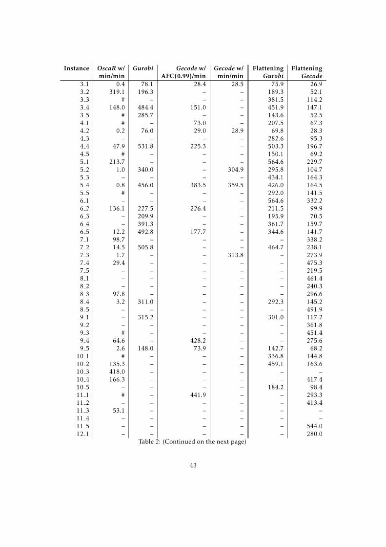
Instance OscaR w/ Gurobi Gecode w/ Gecode w/ Flattening Flatteningmin/min AFC(0.99)/min min/min Gurobi Gecode

3 1 0.4 78.1 28.4 28.5 75.9 26.93 2 319.1 196.3 – – 189.3 52.13 3 # – – – 381.5 114.23 4 148.0 484.4 151.0 – 451.9 147.13 5 # 285.7 – – 143.6 52.54 1 # – 73.0 – 207.5 67.34 2 0.2 76.0 29.0 28.9 69.8 28.34 3 – – – – 282.6 95.34 4 47.9 531.8 225.3 – 503.3 196.74 5 # – – – 150.1 69.25 1 213.7 – – – 564.6 229.75 2 1.0 340.0 – 304.9 295.8 104.75 3 – – – – 434.1 164.35 4 0.8 456.0 383.5 359.5 426.0 164.55 5 # – – – 292.0 141.56 1 – – – – 564.6 332.26 2 136.1 227.5 226.4 – 211.5 99.96 3 – 209.9 – – 195.9 70.56 4 – 391.3 – – 361.7 159.76 5 12.2 492.8 177.7 – 344.6 141.77 1 98.7 – – – – 338.27 2 14.5 505.8 – – 464.7 238.17 3 1.7 – – 313.8 – 273.97 4 29.4 – – – – 475.37 5 – – – – – 219.58 1 – – – – – 461.48 2 – – – – – 240.38 3 97.8 – – – – 296.68 4 3.2 311.0 – – 292.3 145.28 5 – – – – – 491.99 1 – 315.2 – – 301.0 117.29 2 – – – – – 361.89 3 # – – – – 451.49 4 64.6 – 428.2 – – 275.69 5 2.6 148.0 73.9 – 142.7 68.2

10 1 # – – – 336.8 144.810 2 135.3 – – – 459.1 163.610 3 418.0 – – – – –10 4 166.3 – – – – 417.410 5 – – – – 184.2 98.411 1 # – 441.9 – – 293.311 2 – – – – – 413.411 3 53.1 – – – – –11 4 – – – – – –11 5 – – – – – 544.012 1 – – – – – 280.0

Table 2: (Continued on the next page)

43

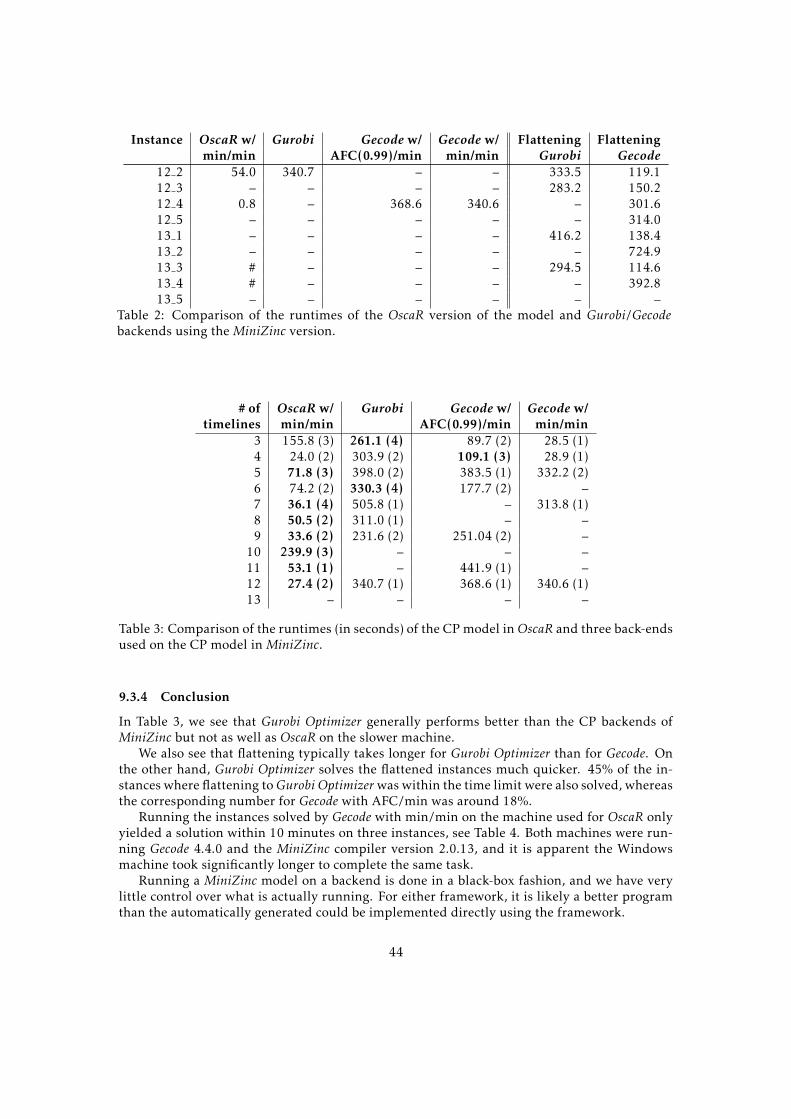
Instance OscaR w/ Gurobi Gecode w/ Gecode w/ Flattening Flatteningmin/min AFC(0.99)/min min/min Gurobi Gecode

12 2 54.0 340.7 – – 333.5 119.112 3 – – – – 283.2 150.212 4 0.8 – 368.6 340.6 – 301.612 5 – – – – – 314.013 1 – – – – 416.2 138.413 2 – – – – – 724.913 3 # – – – 294.5 114.613 4 # – – – – 392.813 5 – – – – – –

Table 2: Comparison of the runtimes of the OscaR version of the model and Gurobi/Gecodebackends using the MiniZinc version.

# of OscaR w/ Gurobi Gecode w/ Gecode w/timelines min/min AFC(0.99)/min min/min

3 155.8 (3) 261.1 (4) 89.7 (2) 28.5 (1)4 24.0 (2) 303.9 (2) 109.1 (3) 28.9 (1)5 71.8 (3) 398.0 (2) 383.5 (1) 332.2 (2)6 74.2 (2) 330.3 (4) 177.7 (2) –7 36.1 (4) 505.8 (1) – 313.8 (1)8 50.5 (2) 311.0 (1) – –9 33.6 (2) 231.6 (2) 251.04 (2) –

10 239.9 (3) – – –11 53.1 (1) – 441.9 (1) –12 27.4 (2) 340.7 (1) 368.6 (1) 340.6 (1)13 – – – –

Table 3: Comparison of the runtimes (in seconds) of the CPmodel inOscaR and three back-endsused on the CP model in MiniZinc.

9.3.4 Conclusion

In Table 3, we see that Gurobi Optimizer generally performs better than the CP backends ofMiniZinc but not as well as OscaR on the slower machine.

We also see that flattening typically takes longer for Gurobi Optimizer than for Gecode. Onthe other hand, Gurobi Optimizer solves the flattened instances much quicker. 45% of the in-stances where flattening toGurobi Optimizerwas within the time limit were also solved, whereasthe corresponding number for Gecode with AFC/min was around 18%.

Running the instances solved by Gecode with min/min on the machine used for OscaR onlyyielded a solution within 10 minutes on three instances, see Table 4. Both machines were run-ning Gecode 4.4.0 and the MiniZinc compiler version 2.0.13, and it is apparent the Windowsmachine took significantly longer to complete the same task.

Running a MiniZinc model on a backend is done in a black-box fashion, and we have verylittle control over what is actually running. For either framework, it is likely a better programthan the automatically generated could be implemented directly using the framework.

44

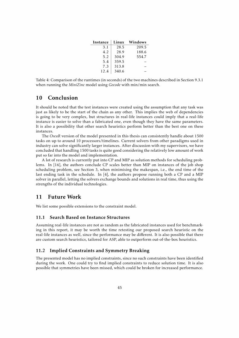
Instance Linux Windows3 1 28.5 209.54 2 28.9 188.65 2 304.9 554.75 4 359.5 –7 3 313.8 –

12 4 340.6 –

Table 4: Comparison of the runtimes (in seconds) of the twomachines described in Section 9.3.1when running the MiniZinc model using Gecode with min/min search.

10 ConclusionIt should be noted that the test instances were created using the assumption that any task wasjust as likely to be the start of the chain as any other. This implies the web of dependenciesis going to be very complex, but structures in real-life instances could imply that a real-lifeinstance is easier to solve than a fabricated one, even though they have the same parameters.It is also a possibility that other search heuristics perform better than the best one on theseinstances.

The OscaR version of the model presented in this thesis can consistently handle about 1500tasks on up to around 10 processors/timelines. Current solvers from other paradigms used inindustry can solve significantly larger instances. After discussion with my supervisors, we haveconcluded that handling 1500 tasks is quite good considering the relatively low amount of workput so far into the model and implementation.

A lot of research is currently put into CP and MIP as solution methods for scheduling prob-lems. In [16], the authors conclude CP scales better than MIP on instances of the job shopscheduling problem, see Section 3, when minimising the makespan, i.e., the end time of thelast ending task in the schedule. In [4], the authors propose running both a CP and a MIPsolver in parallel, letting the solvers exchange bounds and solutions in real time, thus using thestrengths of the individual technologies.

11 Future WorkWe list some possible extensions to the constraint model.

11.1 Search Based on Instance StructuresAssuming real-life instances are not as random as the fabricated instances used for benchmark-ing in this report, it may be worth the time retesting our proposed search heuristic on thereal-life instances as well, since the performance may be different. It is also possible that thereare custom search heuristics, tailored for ASP, able to outperform out-of-the-box heuristics.

11.2 Implied Constraints and Symmetry BreakingThe presented model has no implied constraints, since no such constraints have been identifiedduring the work. One could try to find implied constraints to reduce solution time. It is alsopossible that symmetries have been missed, which could be broken for increased performance.

45

11.3 OptimisationIn this report, we have only made attempts to create a model testing feasibility by trying to finda feasible schedule. In an extension, one could instead modify the presented model to find an,in some sense, optimal schedule. For instance, one could let T be a variable and minimise it,thus maximising the number of finished cycles per time unit.

11.4 Limited Discrepancy SearchLimited discrepancy search (LDS) [12] uses the following idea: if we are doing a tree search andare able to sort the branches by the probability that we will find a solution in that branch,putting the best branch to the left, we can instruct the solver to first search all the leftmostbranches and gradually try branches to the right. For instance, assume we have a problemwhere variables can take values in 1..10 and each node branches into 10 subtrees, one for eachvalue. Furthermore, say that we think that a lot of the variables should be 1. We can then firsttry “all variables are 1”, then all branches having “all 1 except one”, then “all 1 except 2” andso on.

Assume we are in the middle of running a CP solver for the ASP, branching using min/min,where some of the variables, but not all, have been fixed. The next variable used to branch on,say x, is then going to be given its smallest value in the left branch, and in the right branchthe solver is going to remove that smallest value. In this particular problem, there is a highprobability the domain is one or a few ranges of values.

Given that the lowest value in the domain of x does not work, the conditional probabilitythe next lowest value in the domain does work should be slim. Whether a task starts at a or a+1is a small difference for large values of the timeline length. In other words, it could be a goodidea to try LDS.

LDS is patented in the USA, and it is therefore necessary to acquire a licence for using LDSthere. The patent holder, according to [28], has ensured all applications for a non-commerciallicence will be granted.

46

References[1] Ahmad Al-Sheikh. ‘Resource Allocation in Hard Real-Time Avionic Systems:

Scheduling and Routing Problems’. PhD thesis. INSA de Toulouse, France, 2011.

[2] Frederic Boussemart, Guillaume Cavory and Christophe Lecoutre. ‘Solving the cyclic jobshop scheduling problem with linear precedence constraints using CP techniques’. In:Systems, Man and Cybernetics, 2002 IEEE International Conference on. Vol. 7. IEEE, 2002.

[3] Denise L. Draper et al. ‘Cyclic Scheduling’. In: Proceedings of the 16th International JointConference on Artificial Intelligence. Vol. 2. Morgan Kaufmann Publishers Inc, 1999, pp. 1016–1021.

[4] Daniel Fontaine, Laurent Michel and Pascal Van Hentenryck. ‘Parallel Composition ofScheduling Solvers’. In: CP-AI-OR 2016. Ed. by Claude-Guy Quimper. Vol. 9676. LectureNotes in Computer Science. Springer, 2016, pp. 159–169.

[5] Steven Gay et al. ‘Conflict Ordering Search for Scheduling Problems’. In: Principles andPractice of Constraint Programming: 21st International Conference, CP 2015. Ed. by GillesPesant. Vol. 9255. Lecture Notes in Computer Science. Springer, 2015, pp. 140–148.

[6] Gecode Team. Gecode: A Generic Constraint Development Environment. 2006. url: http://www.gecode.org.

[7] Global Constraint Catalog. http://sofdem.github.io/gccat/. Accessed: 2016-01-28.

[8] Global Constraint Catalog, specification of Disjunctive. http : / / sofdem . github . io /gccat/gccat/Cdisjunctive_or_same_start.html. Accessed: 2016-01-28.

[9] Gurobi Optimization Inc. Gurobi Optimizer Reference Manual. 2015. url: http://www.gurobi.com.

[10] Claire Hanen. ‘Study of a NP-hard cyclic scheduling problem: The recurrent job-shop’.In: European Journal of Operational Research 72 (1994), pp. 82–101.

[11] Claire Hanen and Alix Munier. ‘Cyclic Scheduling on Parallel Processors: An Overview’.In: Scheduling Theory and Its Applications. John Wiley & Sons, 1995. Chap. 9.

[12] William D. Harvey and Matthew L. Ginsberg. ‘Limited discrepancy search’. In: IJCAI (1).1995, pp. 607–615.

[13] Trevor Hastie, Robert Tibshirani and Jerome Friedman. The Elements of Statistical Learning– Data Mining, Inference, and Prediction. Second edition. Springer, 2009, pp. 587–588.

[14] Tin Kam Ho. ‘Random Decision Forests’. In: Third International Conference on DocumentAnalysis and Recognition (Vol. 1). ICDAR ’95. IEEE Computer Society, 1995, pp. 278–282.

[15] Hermann Kopetz. Real-Time Systems: Design Principles for Distributed Embedded Applica-tions. Second edition. Springer Science & Business Media, 2011.

[16] Wen-Yang Ku and J. Christopher Beck. Revisiting Off-the-Shelf Mixed Integer Programmingand Constraint Programming Models for Job Shop Scheduling. Tech. rep. MIE-OR-TR2014-01. University of Toronto, Canada, 2014. url: https://mie.utoronto.ca/research/technical-reports/reports/JSP.pdf.

[17] Jean-Louis Lauriere. ‘A Language and a Program for Stating and Solving CombinatorialProblems.’ In: Artificial Intelligence 10.1 (1978), pp. 29–127.

[18] Christophe Lecoutre et al. ‘Reasoning from last conflict(s) in constraint programming’.In: Artificial Intelligence 173.18 (2009), pp. 1592–1614.

47

http://www.gecode.org

http://www.gecode.org

http://sofdem.github.io/gccat/

http://sofdem.github.io/gccat/gccat/Cdisjunctive_or_same_start.html

http://sofdem.github.io/gccat/gccat/Cdisjunctive_or_same_start.html

http://www.gurobi.com

http://www.gurobi.com

https://mie.utoronto.ca/research/technical-reports/reports/JSP.pdf

https://mie.utoronto.ca/research/technical-reports/reports/JSP.pdf

[19] Kim Marriot and Peter J. Stuckey. A MiniZinc Tutorial. http://www.minizinc.org/downloads/doc-latest/minizinc-tute.pdf. 2015.

[20] MiniZinc website. http://www.minizinc.org/. Accessed: 2016-01-26. 2015.

[21] Alix Munier. ‘The Basic Cyclic Scheduling Problem with Linear Precedence Constraints’.In: Discrete Applied Mathematics 64.3 (1996), pp. 219–238.

[22] OscaR Team. OscaR: Scala in OR. Available from http://www.oscarlib.org. 2012.

[23] Claude Le Pape et al. ‘Time-versus-Capacity Compromises in Project Scheduling’. In:Proceedings of the Thirteenth Workshop of the U.K. Planning Special Interest Group. 1994.url: http://citeseerx.ist.psu.edu/viewdoc/download?doi=10.1.1.57.4187&rep=rep1&type=pdf.

[24] R Development Core Team. R: A Language and Environment for Statistical Computing.ISBN 3-900051-07-0. R Foundation for Statistical Computing. Vienna, Austria, 2008. url:http://www.R-project.org.

[25] James W. Ramsey. Integrated Modular Avionics: Less is More.http://www.aviationtoday.com/av/commercial/Integrated-Modular-Avionics-Less-is-More_8420.html. Accessed: 2016-03-01. 2007.

[26] Jean-Charles Regin. ‘A filtering algorithm for constraints of difference in CSPs’. In:AAAI 1994.Ed. by Barbara Hayes-Roth and Richard E. Korf. AAAI Press, 1994, pp. 362–367.

[27] Lior Rokach and Oded Maimon. ‘Top-Down Induction of Decision Trees Classifiers – ASurvey’. In: Transactions on Systems, Man, and Cybernetics. Vol. 35. IEEE, 2005, pp. 476–487.

[28] Christian Schulte. Message to the Gecode users group: Licensing information regarding LDS.Accessed: 2016-06-02. url: http://www.gecode.org/pipermail/users/2010-October/003076.html.

[29] Wind River Systems. ARINC 653 – An Avionics Standard for Safe, Partitioned Systems.http : / / www . computersociety . it / wp - content / uploads / 2008 / 08 / ieee - cc -arinc653_final.pdf. Accessed: 2016-03-01. 2008.

48

http://www.minizinc.org/downloads/doc-latest/minizinc-tute.pdf

http://www.minizinc.org/downloads/doc-latest/minizinc-tute.pdf

http://www.minizinc.org/

http://citeseerx.ist.psu.edu/viewdoc/download?doi=10.1.1.57.4187&rep=rep1&type=pdf

http://citeseerx.ist.psu.edu/viewdoc/download?doi=10.1.1.57.4187&rep=rep1&type=pdf

http://www.R-project.org

http://www.aviationtoday.com/av/commercial/Integrated-Modular-Avionics-Less-is-More_8420.html

http://www.aviationtoday.com/av/commercial/Integrated-Modular-Avionics-Less-is-More_8420.html

http://www.gecode.org/pipermail/users/2010-October/003076.html

http://www.gecode.org/pipermail/users/2010-October/003076.html

http://www.computersociety.it/wp-content/uploads/2008/08/ieee-cc-arinc653_final.pdf

http://www.computersociety.it/wp-content/uploads/2008/08/ieee-cc-arinc653_final.pdf

pre-runtime scheduling of an avionics system -...

Documents