precaution versus mercantilism: reserve accumulation ... · pdf filemdg3 ita3 phl2 fin3 isr2...
TRANSCRIPT

Precaution Versus Mercantilism:Reserve Accumulation, Capital Controls,
and the Real Exchange Rate
Woo Jin Choi † Alan M. Taylor ‡
† Korea Development Institute
‡ University of California, Davis; NBER; and CEPR
CEPR-SNB-BoI ConferenceForeign Exchange Market Intervention: Conventional or Unconventional Policy?
Jerusalem7–8 December 2017
0 / 34

Motivating Questions
How does a nation’s current wealth affect its future RER & trade balances?
• Traditional answer is higher NFA =⇒ stronger RER, lower TB (Hume)
• Standard theory: neoclassical model of private sector, TBt = −r∗NFA0
• Standard evidence: seminal work by Lane and Milesi-Ferretti (2002/04)
• Logic: if you become wealthier you want to consume out of that wealth
Might this view be incomplete?
• New assumptions: role of government and its motives
• Some NFA wealth is not held by private sector (reserves)
• Government may have motives to prefer NFA ↑ (insurance/“precaution”)
• Government may have motives to prefer TB ↑ (externality/“mercantilism”)
What does this paper do?
• Break the simple association between NFA and TB
• Revisit/extend the LMF results with evidence that NFAxR 6= RSRV
• Optimal policy on 2 dimensions will require 2 instruments
• Present a theoretical model of capital controls and reserve accumulation
1 / 34

Reserve Accumulation: Facts
One of the most striking phenomena in global macro for last two decades.• By 2011 global reserves exceeded $10 trillion (14% of World GDP).• Large increase concentrated in developing countries.
01
02
03
0P
erc
en
tag
e o
f G
DP
(u
nw
eig
hte
d)
1980 1990 2000 2010Year
Developing Advanced
Avg. Reserve Accumulation / GDP (Source : IMF IFS)
decomposition summary
2 / 34

Reserves Accumulations: Rationales
In theories of reserve accumulation, two motives are usually considered separately:
Mercantilist motive• (Net) export in mfg. increases productivity (learning-by-doing externality).• Amassing reserves devalues real exchange rate, boosts mfg. exports.• Aizenman and Lee (2007), Jeanne (2013), Benigno and Fornaro (2012),
Korinek and Serven (2016).
Precautionary motive• Precautionary stockpiling as an insurance against BOP/financial crisis.• Amassing reserves creates buffer for using in a sudden stop/flight.• Obstfeld, Shambaugh and Taylor (2010), Jeanne and Ranciere (2011),
Bianchi, Hatchondo, and Martinez (2016).
We construct a simple integrated theoretical framework to account for realexchange rate determination incorporating BOTH views in one model.
We compare the predictions of the model to our data driven empirical findings.
3 / 34

Reserves Accumulations: Rationales
In theories of reserve accumulation, two motives are usually considered separately:
Mercantilist motive• (Net) export in mfg. increases productivity (learning-by-doing externality).• Amassing reserves devalues real exchange rate, boosts mfg. exports.• Aizenman and Lee (2007), Jeanne (2013), Benigno and Fornaro (2012),
Korinek and Serven (2016).
Precautionary motive• Precautionary stockpiling as an insurance against BOP/financial crisis.• Amassing reserves creates buffer for using in a sudden stop/flight.• Obstfeld, Shambaugh and Taylor (2010), Jeanne and Ranciere (2011),
Bianchi, Hatchondo, and Martinez (2016).
We construct a simple integrated theoretical framework to account for realexchange rate determination incorporating BOTH views in one model.
We compare the predictions of the model to our data driven empirical findings.3 / 34

Preview: Model Intuition
Two distortions: financial crisis cost (ξ) and LBD externality (ν).Two policy instruments: reserves (rsrv) and capital controls (tax indexed by κ).
Start from baseline: no financial crisis (ξ = 0), no LBD externality (ν = 0).
Laissez faire. Government chooses no reserves (rsrv = 0) and no capital controls(κ = 0), and so the laissez faire equilibrium (0,0) below is socially optimal.
0
Polic
y: ca
pital
cont
rol
0 Policy: reserve accumulation
4 / 34

Preview: Model Intuition
Deviate from baseline: increase crisis cost (ξ ↑), no LBD externality (ν = 0).
Pure precautionary motive. Government increases reserves (rsrv ↑) but uses no capitalcontrols (κ = 0), and the socially optimal equilibrium moves to the right.
0
Polic
y: ca
pital
cont
rol
0 Policy: reserve accumulation
5 / 34

Preview: Model Intuition
Deviate from baseline: no financial crisis (ξ = 0), increase LBD externality (ν ↑).
Pure mercantilist motive. Government increases reserves (rsrv ↑) and uses capitalcontrols (κ ↑), and the socially optimal equilibrium moves up and right.
(Why? Ricardian equivalence, so controls are needed to ensure offsetting effects ofprivate capital flows are only partial, then externality kicks in via TB ↑ and RER deval.)
0
Polic
y: ca
pital
cont
rol
0 Policy: reserve accumulation
6 / 34

Preview: Model Intuition
Deviate more: when 2 distortions are present (ξ ↑, ν ↑).
Policy tradeoff. Like before, but both policies are costly so there is a tradeoff when weare away from the extreme cases when only 0 or 1 distortions are present.
(Clearest for precautionary motive: when this rises, all else equal, the policymakersusbtitutes and the mercantilist motive is dialed back: reserves rise on net, but capitalcontrols are relaxed)
0
Polic
y: ca
pital
cont
rol
0 Policy: reserve accumulation 7 / 34
Our Goal
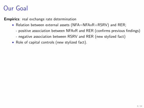
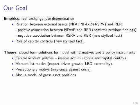
Empirics: real exchange rate determination
• Relation between external assets (NFA=NFAxR+RSRV) and RER;
- positive association between NFAxR and RER (confirms previous findings)
- negative association between RSRV and RER (new stylized fact)
• Role of capital controls (new stylized fact).
Theory: closed form solutions for model with 2 motives and 2 policy instruments
• Capital account policies – reserve accumulations and capital controls.
• Mercantilist motive (export-driven growth, LBD externality).
• Precautionary motive (insurance against crisis).
• Also, a model of gross asset positions.
Additional empirics: trade balance v. growth relationship consistent with theory
• association between capital account policies and trade surplus.
• association between capital account policies and growth of GDP / TFP.
8 / 34
Our Goal
Empirics: real exchange rate determination
• Relation between external assets (NFA=NFAxR+RSRV) and RER;
- positive association between NFAxR and RER (confirms previous findings)
- negative association between RSRV and RER (new stylized fact)
• Role of capital controls (new stylized fact).
Theory: closed form solutions for model with 2 motives and 2 policy instruments
• Capital account policies – reserve accumulations and capital controls.
• Mercantilist motive (export-driven growth, LBD externality).
• Precautionary motive (insurance against crisis).
• Also, a model of gross asset positions.
Additional empirics: trade balance v. growth relationship consistent with theory
• association between capital account policies and trade surplus.
• association between capital account policies and growth of GDP / TFP.
8 / 34

Empirics: Data
• 22 advanced countries and 53 developing countries, covering 1975 to 2007(2011).
• Data Source : IFS-IMF, DOTS-IMF, External Wealth of Nations Mark IIfrom Lane and Milesi-Ferretti (2007), Penn World Table (7,9), WorldBank, OECD, and BIS Statistics, Barro and Lee (2013), Chinn and Ito(2008), Edwards (2007), Fernandez, Klein, Rebucci, Schindler, andUribe(2015), Quinn and Toyota (2008).
• We split the sample into subperiods (as in LMF):
1975–1985 : Period 11986–1996 : Period 21997–2007 : Period 32008–2011 : Period 4
9 / 34
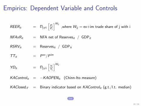
Empirics: Dependent Variable and Controls
REERit = Πj 6=i
[Pi
Pj
]Wij
,where Wij = ex+im trade share of j with i
NFAxRit = NFA net of Reservesit / GDPit
RSRVit = Reservesit / GDPit
TTit = Pex/P im
YDit = Πj 6=i
[Yi
Yj
]Wij
KAControlit = −KAOPENit (Chinn-Ito measure)
KAClosediT = Binary indicator based on KAControlit (g.t./l.t. median)
link
10 / 34
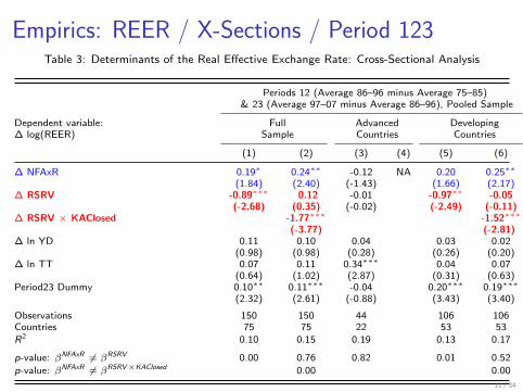
Empirics: REER / X-Sections / Period 123Table 3: Determinants of the Real Effective Exchange Rate: Cross-Sectional Analysis
Periods 12 (Average 86–96 minus Average 75–85)& 23 (Average 97–07 minus Average 86–96), Pooled Sample
Dependent variable: Full Advanced Developing∆ log(REER) Sample Countries Countries
(1) (2) (3) (4) (5) (6)
∆ NFAxR 0.19∗ 0.24∗∗ -0.12 NA 0.20 0.25∗∗
(1.84) (2.40) (-1.43) (1.66) (2.17)∆ RSRV -0.89∗∗∗ 0.12 -0.01 -0.97∗∗ -0.05
(-2.68) (0.35) (-0.02) (-2.49) (-0.11)∆ RSRV × KAClosed -1.77∗∗∗ -1.52∗∗∗
(-3.77) (-2.81)∆ ln YD 0.11 0.10 0.04 0.03 0.02
(0.98) (0.98) (0.28) (0.26) (0.20)∆ ln TT 0.07 0.11 0.34∗∗∗ 0.04 0.07
(0.64) (1.02) (2.87) (0.31) (0.63)Period23 Dummy 0.10∗∗ 0.11∗∗∗ -0.04 0.20∗∗∗ 0.19∗∗∗
(2.32) (2.61) (-0.88) (3.43) (3.40)
Observations 150 150 44 106 106Countries 75 75 22 53 53R2 0.10 0.15 0.19 0.13 0.17
p-value: βNFAxR 6= βRSRV 0.00 0.76 0.82 0.01 0.52
p-value: βNFAxR 6= βRSRV×KAClosed 0.00 0.00
11 / 34

Empirics: REER / X-Sections / Period 123
Figure 1a: Real Exchange Rate Determination: Developing Countries, Period 123 (1975-2007)
PRY3
NGA2
SYR2
MDG2
GMB3JOR2BDI3
CIV2KOR3
BDI2CHN3
TTO2THA2
GRC3PRT3
THA3JOR3
TGO3
NZL2
GMB2HND2
SLB2
ISL3ESP3FIN3
TUR3
NER2
ARG3
IDN2
ECU2IDN3
IND3GBR3
LKA2NPL2CYP2BRA3CMR2AUS2
CHN2
DZA3
NLD3KEN2PHL3
TZA2
MAR2SEN3
NPL3
BOL3
COL3FRA2
DOM2
SWE2GTM3
BHR3
USA3HND3
IRN3
AUT3
FIN2
SAU3PAK3NZL3
MYS2
AUS3CYP3ITA3TTO3
IND2TUR2
ISL2
VEN2
USA2
CMR3
GRC2DOM3
DEU3COL2
PHL2SEN2
MYS3
MEX2
ESP2
FJI3
BOL2
FRA3
MEX3ITA2URY3
SWE3
EGY3
CAN2
MAR3GBR2PER3
ISR3
DNK2EGY2
LKA3NLD2
DZA2CHL2
PER2
AUT2
PAK2
FJI2URY2
NER3
ARG2
PNG2CHL3
GTM2
BEL2
JPN3
SYR3CHE2
PRY2
ECU3PRT2IRL2TZA3DEU2
JPN2
DNK3
IRN2
SLB3
KEN3
JAM2
KOR2
CRI2CRI3
VEN3
ISR2
CAN3
MDG3NOR2
LBY3
BRA2
PNG3CIV3IRL3
BEL3
JAM3
TGO2CHE3
LBY2
NOR3
NGA3
SAU2
BHR2
-1-.5
0.5
1d
ln(R
EER)
-1 -.5 0 .5 1dNFAxR
coef = .23685162, (robust) se = .09866104, t = 2.4
(a) dNFAxR
12 / 34

Empirics: REER / X-Sections / Period 123
Figure 1b: Real Exchange Rate Determination: Developing Countries, Period 123 (1975-2007)
TTO2
SAU2
BHR3IRL3
PRT3
JOR2ESP3NLD3
BHR2
IRL2
DEU3BEL3
GBR3AUT3
GRC3
ITA3SWE3ECU3ISR2
CHE2
DOM3
DEU2CHL3FIN3
USA3
CRI3FRA3LKA3CHN3CYP3KOR2CYP2CHE3
KOR3
TGO3IND3FJI3
NER3
NZL3
CHN2EGY3
TUR3
BRA3
VEN2
COL3
PAK3ISL3ARG3
PRY2
GTM2
PRY3THA3BDI3AUS3
DOM2
FRA2
KEN2NPL3TZA3
IRN3
AUT2VEN3
MDG3
KEN3
CMR3SEN3IND2
MAR3
NGA3HND3
PHL3
SYR3
NOR3
THA2
ITA2
PAK2
CIV3LKA2CAN3
EGY2
TUR2COL2
HND2
BRA2JPN2
PNG3
GBR2BDI2USA2
MAR2NPL2
CHL2BOL2
BEL2
CRI2FJI2
SLB3CMR2SEN2
TZA2
ARG2ISL2
PNG2TGO2
DZA2
SYR2IRN2
PHL2CAN2
CIV2
NER2
NGA2
NLD2
ECU2MDG2SLB2URY2
IDN2
MEX3AUS2
LBY2
GMB3
PER2
DNK2
LBY3DZA3MEX2
FIN2ESP2GTM3SWE2
JAM2
NOR2DNK3
GRC2NZL2
URY3JAM3
IDN3BOL3
GMB2ISR3
PER3
JPN3MYS2
SAU3
PRT2
MYS3
TTO3
JOR3
-1-.5
0.5
1d
ln(R
EER)
-.3 -.2 -.1 0 .1 .2dRSRV
coef = .12011033, (robust) se = .34743816, t = .35
(b) dRSRV
13 / 34

Empirics: REER / X-Sections / Period 123
Figure 1c: Real Exchange Rate Determination: Developing Countries, Period 123 (1975-2007)
JOR3
TTO3
MYS3SAU3
PRT2
ISR3PER3
JPN3BOL3MYS2IDN3
JAM3URY3
PNG2DNK3
IRN2
NOR3
NOR2GTM3GMB2MEX3
CAN3
ESP2
JAM2
NZL2
TGO3
DNK2VEN3GRC2
BRA2
SWE2
CHE3TGO2
PRY2
FIN2
CRI3
DZA2PAK2
MEX2
SLB2
AUS3
NER3
URY2
LBY2
JPN2
NLD2NZL3CMR2
CHL3LKA3CAN2BEL2FRA3FJI3CYP2
PER2
ISL2
BEL3
GBR2ITA2
PNG3
KOR2BDI3
USA3ISL3HND2USA2
IND2
SLB3KEN2ECU3
AUT2
NGA2
AUS2
IDN2
ECU2
SWE3
ARG2MDG3ITA3PHL2FIN3ISR2COL3SEN2AUT3
BHR2TUR2
BOL2DEU3COL2
DEU2
FRA2
SYR2
EGY3
CIV2
GBR3
GTM2
DOM3GMB3
KEN3
VEN2
CHE2IRL2GRC3
FJI2
CYP3
CRI2CMR3
BRA3
CIV3LKA2PAK3NPL2
TZA2
NER2TZA3
DOM2
PRY3
CHN2
NLD3MAR2IRL3
ESP3NPL3
TUR3
ARG3PHL3
MDG2
IRN3
NGA3BDI2
CHL2
IND3
SEN3
THA2JOR2THA3
SYR3
PRT3MAR3EGY2
BHR3
KOR3CHN3HND3
SAU2
DZA3LBY3
TTO2
-1.5
-1-.5
0.5
1d
ln(R
EER)
-.2 -.1 0 .1 .2dRSRV * KAClosed
coef = -1.7728668, (robust) se = .47044226, t = -3.77
(c) dRSRV * KAClosed
14 / 34

Empirics: REER / X-Sections / Period 12
Table 4: Determinants of the Real Effective Exchange Rate: Cross-Sectional Analysis
Period 12 (Average 86–96 minus Average 75–85)
Dependent variable: Full Advanced Developing∆ log(REER) Sample Countries Countries
(1) (2) (3) (4) (5) (6)
∆ NFAxR 0.38∗∗ 0.39∗∗ 0.19 0.15 0.33∗ 0.34∗
(2.19) (2.22) (0.73) (0.56) (1.73) (1.75)∆ RSRV 0.32 0.62 0.21 0.10 0.12 0.35
(0.50) (0.81) (0.31) (0.14) (0.18) (0.42)∆ RSRV × KAClosed -1.53 1.79 -1.01
(-0.86) (0.95) (-0.54)∆ ln YD -0.10 -0.09 -0.33 -0.25 -0.18 -0.17
(-0.60) (-0.56) (-0.81) (-0.54) (-1.05) (-1.03)∆ ln TT 0.43∗∗ 0.40∗∗ 0.45∗∗ 0.49∗∗ 0.36∗ 0.34∗
(2.47) (2.30) (2.52) (2.55) (1.74) (1.69)
Observations 75 75 22 22 53 53Countries 75 75 22 22 53 53R2 0.16 0.17 0.17 0.18 0.12 0.13
p-value: βNFAxR 6= βRSRV 0.93 0.77 0.98 0.95 0.79 0.99
p-value: βNFAxR 6= βRSRV×KAClosed 0.29 0.42 0.49
15 / 34

Empirics: REER / X-Sections / Period 23
Table 5: Determinants of the Real Effective Exchange Rate: Cross-Sectional Analysis
Period 23 (Average 97–07 minus Average 86–96)
Dependent variable: Full Advanced Developing∆ log(REER) Sample Countries Countries
(1) (2) (3) (4) (5) (6)
∆ NFAxR 0.15∗∗ 0.19∗∗∗ -0.17 NA 0.22∗∗ 0.28∗∗∗
(2.12) (2.83) (-1.50) (2.21) (2.96)∆ RSRV -0.96∗∗∗ -0.23 -0.12 -1.06∗∗∗ -0.08
(-3.37) (-0.62) (-0.14) (-2.72) (-0.15)∆ RSRV × KAClosed -1.06∗∗ -1.31∗∗
(-2.33) (-2.40)∆ ln YD 0.13 0.14∗ -0.03 0.16 0.15
(1.57) (1.74) (-0.11) (1.62) (1.52)∆ ln TT -0.16 -0.14 0.34 -0.15 -0.14
(-1.22) (-1.12) (1.69) (-1.10) (-1.05)
Observations 75 75 22 53 53Countries 75 75 22 53 53
R2 0.18 0.22 0.16 0.18 0.24
p-value: βNFAxR 6= βRSRV 0.00 0.28 0.96 0.01 0.50
p-value: βNFAxR 6= βRSRV×KAClosed 0.01 0.01
16 / 34

Other Specifications and Robustness
Annual panel with fixed effect; link
• Consistent with cross-sectional analysis, but statistically more significant.
Robustness :
• Continuous, instead of binary, measure of capital controls. link
• Without oil exporters. link
• Other REER measures. link
• Other capital control measures. link
• Crisis periods. link
• Dynamic OLS specification, incorporating possible cointegration betweenvariables.
17 / 34

Basic Model: Exogenous Capital Account Policies
Develop a theory to account for new stylized facts from the empirical work.
Small open economy, 2 goods, 2 periods, 2 financial markets (domestic and int’l).
Infinitesimally small but identical agents.
Consumption good is
ct =
((θT) 1σ cTt
σ−1σ + (θN)
1σ cNt
σ−1σ
) σσ−1
.
Utility maximization
max{cT0,1, cN0,1, d∗, a}
{u(c0) +
1
1 + r∗u(c1)
},
where u(·) is standard CRRA utility function with risk-aversion parameter γ,
18 / 34

Basic Model: Exogenous Capital Account Policies
subject to
cT0 + p0cN0 + a + τ(d∗, κ) ≤ (1 + ω)yT + p0y
N + d∗ + T0,
cT1 + p1cN1 + (1 + r∗)d∗ ≤ (1 + g)yT + p1y
N + (1 + r)a + T1,
where
cTt , cNt T and NT consumption
yT , yN T and NT endowment
pt the price of the nontradable goods in period t
d∗ external private debt
a domestic public asset (= reserves)
ω shock to initial level of wealth (endowment) of T sector
g growth of future endowment of T sector
r∗, r international and domestic interest rates
τ(d∗, κ) “Pigouvian or Tobin” tax on d∗(indexed by policy κ)
Tt government lump-sum transfer (taxes are rebated)
19 / 34
Basic Model: Exogenous Capital Account Policies
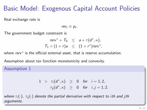
Real exchange rate is
rert ≡ pt .
The government budget constraint is
rsrv∗ + T0 ≤ a + τ(d∗, κ),
T1 + (1 + r)a ≤ (1 + r∗)rsrv∗,
where rsrv∗ is the official external asset, that is reserve accumulation.
Assumption about tax function monotonicity and convexity.
Assumption 1
1 > τi (d∗, κ) ≥ 0 for i = 1, 2,
τij(d∗, κ) ≥ 0 for i , j = 1, 2.
where τi (·), τij(·) denote the partial derivative with respect to ith and jtharguments.
20 / 34
Basic Model: Exogenous Capital Account Policies
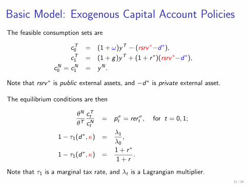
The feasible consumption sets are
cT0 = (1 + ω)yT − (rsrv∗−d∗),cT1 = (1 + g)yT + (1 + r∗)(rsrv∗−d∗),
cN0 = cN1 = yN .
Note that rsrv∗ is public external assets, and −d∗ is private external asset.
The equilibrium conditions are then
θN
θTcTtcNt
= pσt = rerσt , for t = 0, 1;
1− τ1(d∗, κ) =λ1
λ0,
1− τ1(d∗, κ) =1 + r∗
1 + r.
Note that τ1 is a marginal tax rate, and λt is a Lagrangian multiplier.
21 / 34

Basic Model: Propositions - Standard Results
Standard wealth effect:
Proposition 1a
Given the level of reserve accumulation (rsrv∗) and the degree of capital controlparameter (κ), and increase in the current endowment of tradable goods (ω) willcause an appreciation of the current real exchange rate,
∂rer0∂ω
≥ 0.
Proposition 1b
Given the level of reserve accumulation (rsrv∗) and the degree of capital controlparameter (κ), and increase in the current endowment of tradable goods (ω) willcause an increase in NFA ex. Reserves (−d∗)
∂ (−d∗)∂ω
≥ 0.
22 / 34

Basic Model: Propositions - New Results
Reserve accumulation rsrv∗ as a fiscal instrument:
Proposition 2
Given current endowment (ω) and the degree of capital control index (κ),increasing reserve accumulation (rsrv∗) will depreciate the current real exchangerate. That is,
∂rer0∂rsrv∗
≤ 0.
Capital control κ with τ12(·) ≥ 0:
Proposition 3
Given current endowment (ω) and reserve accumulation (rsrv∗), increasing thedegree of capital control index (κ) will depreciate the current real exchange rate,That is,
∂rer0∂κ
≤ 0.
23 / 34

Full Model: Endogenous Capital Account Policies
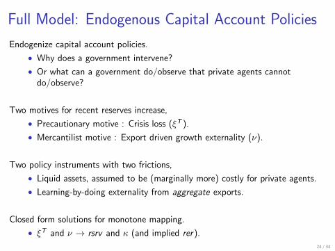
Endogenize capital account policies.
• Why does a government intervene?
• Or what can a government do/observe that private agents cannotdo/observe?
Two motives for recent reserves increase,
• Precautionary motive : Crisis loss (ξT ).
• Mercantilist motive : Export driven growth externality (ν).
Two policy instruments with two frictions,
• Liquid assets, assumed to be (marginally more) costly for private agents.
• Learning-by-doing externality from aggregate exports.
Closed form solutions for monotone mapping.
• ξT and ν → rsrv and κ (and implied rer).
24 / 34

Full Model: Endogenous Capital Account Policies
Endogenize capital account policies.
• Why does a government intervene?
• Or what can a government do/observe that private agents cannotdo/observe?
Two motives for recent reserves increase,
• Precautionary motive : Crisis loss (ξT ).
• Mercantilist motive : Export driven growth externality (ν).
Two policy instruments with two frictions,
• Liquid assets, assumed to be (marginally more) costly for private agents.
• Learning-by-doing externality from aggregate exports.
Closed form solutions for monotone mapping.
• ξT and ν → rsrv and κ (and implied rer).
24 / 34

Full Model: Endogenous Capital Account Policies :
Setup
First period t = 0 is divided into two sub-periods;
• t = 0− : Decision / contract for financial transaction.
• t = 0+ : State realizes. Financial contract needs to be honored.
At t = 0+, crisis with fixed probability π,
• Output loss : ξT (ξN) share of in tradable (nontradable) endowments.
• Exclusion from international financial market.
• But government rsrv can be liquidated (at a cost η) if crisis occurs.
Learning by doing externality;
• g = g + g(ex0, ν), if no crisis,
• g = g , if crisis.
25 / 34

Full Model: Endogenous Capital Account Policies
Constrained Social Planner’s Problem
Feasible consumption sets (where hats denote the crisis state)
cT0 = (1 + ω)yT − (rsrv∗ − d∗),
cT1 = (1 + g + g(ex0, ν)) yT + (1 + r∗)(rsrv∗ − d∗),
cT0 = (1 + ω − ξT )yT − η(rsrv∗, yT )− (−d∗),cT1 = (1 + g)yT + (1 + r∗)(−d∗),
cN0 = yN ,
cN1 = yN ,
cN0 = (1− ξN)yN ,
cN1 = yN .
26 / 34

Full Model: Endogenous Capital Account Policies
Constrained Social Planner’s Problem
Aggregate export,
ex0 = (1 + ω)yT − cT0 = rsrv∗ − d∗.
Growth rate,
g(ex0, ν)yT = ν(rsrv∗ − d∗).
First order conditions for consumption with Lagrange Multipliers,
λ0 =1 + r∗ + ν
1 + r∗λ1,
λ0 =1 + r∗
1 + r∗λ1.
27 / 34

Full Model: Endogenous Capital Account Policies
Constrained Social Planner’s Problem
Seek closed form solutions for rsrv and κ (and implied d and rer).
For tractability now assume also: log utility (γ = 1), unit elasticity between T &NT (σ = 1), and fixed cost for liquidation (η). Then, at the social optimum:
−d∗opt1 =1
2 + r∗(−(1 + g) + (1 + ω) + (−ξT − η)
)· yT ,
rsrv∗opt1 =1
2 + r∗
(ν(1 + g)
1 + r∗ + ν− (−ξT − η)
)· yT ,
reropt0 =θN
θT· 1 + r∗
2 + r∗·(
1 + ω +1 + g
1 + r∗ + ν
)· y
T
yN.
ω : current productivityξT : crisis lossν : growth externalityη : liquidation penalty
28 / 34

Full Model: Endogenous Capital Account Policies
Constrained Social Planner’s Problem
Proposition 4
Fixing all other parameters, if an economy has a higher output loss in a crisis(ξT ), optimal reserve accumulation increases while the real exchange rate is notaffected.
∂rsrv∗opt1
∂ξT=
∂ − d∗opt1
∂ξT> 0,
∂reropt0
∂ξT= 0.
29 / 34

Full Model: Endogenous Capital Account Policies
Constrained Social Planner’s Problem
Proposition 5
Fixing all other parameters, if an economy has a higher growth externality (ν),optimal reserve accumulation increases while the real exchange rate is depreciated.
∂rsrv∗opt1
∂ν> 0,
∂ − d∗opt1
∂ν= 0,
∂reropt0
∂ν< 0.
30 / 34

Full Model: Endogenous Capital Account Policies
Optimal Capital Account Policy
The Optimal Capital Account Policy is to set rsrv∗=rsrv∗opt1 , and optimalcapital control κ satisfying
1− τ1(d∗opt1 , κ) =(1− π)λ∗opt1 + πλ∗opt1
(1− π)λ∗opt0 + πλ∗opt0
.
Theorem 1 (Precaution Versus Mercantilism)
All else equal, if an economy has a higher output loss in a crisis (ξT ), the optimaldegree of capital control decreases. And if an economy has a higher growthexternality (ν), the optimal degree of capital control increases. That is,
∂κopt
∂ξT≤ 0, and
∂κopt
∂ν≥ 0.
link
31 / 34

Capital Account Policy and Growth
Capital account policy and growth.
• Is the policy statistically associated with growth?
Focus on period 23,
• Cross section and annual Panel.
link
32 / 34

Empirics: Capital Account Policy and GrowthTable 17: Cross Section: Capital Account Policy and Growth of Real GDP and TFP
Period 2 and 3 (1986–2007)
Dependent variable: Real GDP per Capita Growth TFP Growth
All w/o Oil All w/o Oil
(1) (2) (3) (4)
∆ RSRV -0.65∗∗ -0.54 -0.47∗∗ -0.61∗∗
(-2.02) (-1.01) (-2.37) (-2.48)∆ RSRV × KAClosed 1.66∗∗∗ 1.33∗ 0.59∗∗ 0.66∗∗
(2.77) (1.80) (2.49) (2.37)Initial Real GDP per capita or TFP 0.06 0.03 -0.54∗∗∗ -0.57∗∗∗
(1.30) (0.59) (-7.28) (-6.04)Schooling 0.03∗∗ 0.03∗ 0.01 0.01
(2.24) (1.90) (1.43) (1.13)Inst. Quality -0.06 -0.03 0.03∗∗∗ 0.03∗
(-1.66) (-0.87) (2.98) (1.80)Trade Openness 0.15∗∗∗ 0.05 0.01 0.01
(3.01) (0.57) (0.56) (0.27)Credit to GDP -0.00 -0.00 -0.00 -0.00
(-0.33) (-0.09) (-0.77) (-0.32)Terms of Trade (% change) 0.09 0.06 0.03 -0.01
(0.97) (0.63) (0.52) (-0.17)
Observations 64 54 61 52Countries 64 54 61 52R2 0.39 0.29 0.70 0.69
33 / 34

Conclusion
We provide new stylized facts.
• Capital account policy – reserves and capital controls – is associated withreal exchange rate depreciation
• And it is more pronounced in developing countries over the last twodecades.
We provide new guidance for real exchange rate determinations.
• The model incorporates both Mercantilist and Precautionary motivestogether.
• Embeds different rationale for private and public external asset holdings.
• Consistent with empirical evidence on NFA, reserves, RER, trade balance,and GDP growth.
34 / 34

Reserve Accumulation : Balance Sheet
DecompositionWe can decompose Net Foreign Asset (NFA)
= Total Foreign Assets - Total Foreign Liabilities
= (FDIA+EQA+DEBTA+Reserve)− (FDIL+EQL+DEBTL)
= Foreign Asset net of Reserve− Foreign Liabilities + RES
= NFAxR + RES.
As of 2011, in developing countries reserve accumulation is
• 22.2% of GDP, 39.8% of Total Foreign Assets, and 143% of DEBTA.
In Advanced countries reserve accumulation is
• 8.9% of GDP, 4.2% of Total Foreign Assets, and 10.7% of DEBTA.
back
34 / 34

Reserve Accumulation : Cross Country EvidenceAs of Year 2011
Percentage of
Rank Country Res (Bil.$) GDP Total Liability Total Asset Debt Asset
1 China 3202.8 42.7 99.8 67.5 331.02 Japan 1258.2 21.3 30.9 16.9 27.93 Saudi Arabia 540.7 80.8 176.5 51.8 197.54 Russia 453.9 22.3 41.3 38.0 123.15 Brazil 350.4 13.4 23.6 46.1 188.06 Korea 304.3 25.3 36.3 40.5 171.67 Hong Kong 285.3 114.8 12.0 9.2 24.88 Switzerland 279.4 40.1 10.5 8.0 18.59 India 271.3 14.9 37.0 66.8 1171.6
10 Singapore 237.5 86.3 13.0 10.1 18.811 Algeria 182.8 91.4 630.7 95.5 2865.612 Thailand 167.4 45.2 53.0 60.6 300.813 Mexico 144.0 12.3 17.8 34.1 90.014 United States 136.9 0.9 0.5 0.6 1.915 Malaysia 131.8 44.2 40.4 39.1 188.016 Indonesia 106.5 11.9 21.7 57.2 298.917 Libya 104.8 302.0 388.2 45.5 158.518 Poland 92.6 17.5 18.9 45.9 270.219 Denmark 81.7 23.9 11.6 10.4 22.720 United Kingdom 79.3 3.1 0.5 0.5 0.921 Turkey 78.3 10.1 15.7 46.2 124.4
back 34 / 34

Reserves, Capital Flows, and Trade FlowsIn our framework, real exchange rate determination is all about forced saving
• If the private agent perceives reserves as their wealth, there is no need todecrease the current consumption (Ricardian Equivalence).
• Thus to force them to decrease consumption, and increase external saving,there need to be capital account restriction.
• We need reserves + capital controls
back
34 / 34
Empirics: Econometric Specification
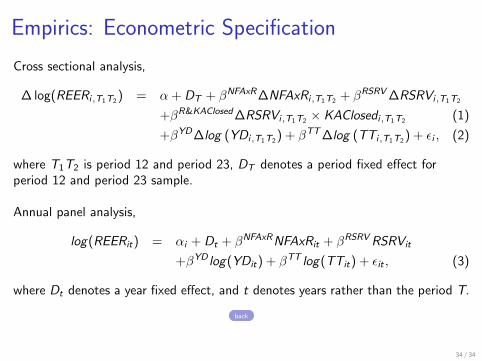
Cross sectional analysis,
∆ log(REERi,T1T2 ) = α + DT + βNFAxR∆NFAxRi,T1T2 + βRSRV ∆RSRVi,T1T2
+βR&KAClosed∆RSRVi,T1T2 × KAClosedi,T1T2 (1)
+βYD∆log (YDi,T1T2 ) + βTT∆log (TTi,T1T2 ) + εi , (2)
where T1T2 is period 12 and period 23, DT denotes a period fixed effect forperiod 12 and period 23 sample.
Annual panel analysis,
log(REERit) = αi + Dt + βNFAxRNFAxRit + βRSRVRSRVit
+βYD log(YDit) + βTT log(TTit) + εit , (3)
where Dt denotes a year fixed effect, and t denotes years rather than the period T.
back
34 / 34

Empirics: REER / Annual Panel / Period 123Table 6: Determinants of the Real Effective Exchange Rate: Annual Panel with Fixed Effects
Period 123 (1975–2007)
Dependent variable: Full Advanced Developing Financially Financially∆ log(REER) Sample Countries Countries Open Closed
(1) (2) (3) (4) (5)
NFAxR 0.17*** -0.03 0.19** 0.12 0.21**(2.74) (-0.63) (2.55) (1.56) (2.47)
RSRV -0.98*** 0.20 -0.89*** -0.24 -1.28***(-3.39) (0.63) (-2.78) (-0.84) (-3.88)
ln YD 0.16** 0.05 0.10 0.22 0.11*(2.10) (0.39) (1.28) (0.91) (1.86)
ln TT -0.03 0.12 -0.06 0.06 -0.08(-0.56) (1.54) (-0.90) (1.07) (-0.90)
Observations 2,475 726 1,749 1,254 1,221Countries 75 22 53 38 37R2 0.188 0.23 0.273 0.092 0.31
p-value: βNFAxR 6= βRSRV 0.000 0.506 0.003 0.257 0.000
back
34 / 34

Empirics: REER / Annual Panel / Period 12Table 7: Determinants of the Real Effective Exchange Rate: Annual Panel with Fixed Effects
Period 12 (1975–1996)
Dependent variable: Full Advanced Developing Financially Financially∆ log(REER) Sample Countries Countries Open Closed
(1) (2) (3) (4) (5)
NFAxR 0.32*** 0.22* 0.30** 0.14 0.42**(2.83) (1.74) (2.40) (1.39) (2.65)
RSRV -0.48* 0.38 -0.57** -0.33 -1.06***(-1.75) (0.88) (-2.04) (-1.13) (-2.95)
ln YD 0.04 -0.10 -0.05 0.42*** -0.21(0.31) (-0.37) (-0.35) (2.85) (-1.51)
ln TT 0.02 0.13 -0.02 0.11 -0.06(0.36) (1.50) (-0.20) (1.42) (-0.55)
Observations 1,650 484 1,166 836 814Countries 75 22 53 38 37R2 0.158 0.26 0.25 0.24 0.209
p-value: βNFAxR 6= βRSRV 0.020 0.725 0.016 0.164 0.001
back
34 / 34

Empirics: REER / Annual Panel / Period 23Table 8: Determinants of the Real Effective Exchange Rate: Annual Panel with Fixed Effects
Period 23 (1986–2007)
Dependent variable: Full Advanced Developing Financially Financially∆ log(REER) Sample Countries Countries Open Closed
(1) (2) (3) (4) (5)
NFAxR 0.13** -0.07 0.17** 0.11** 0.23**(2.21) (-1.57) (2.19) (2.06) (2.65)
RSRV -0.90*** -0.06 -0.91** -0.41* -1.19***(-3.07) (-0.24) (-2.59) (-1.77) (-3.33)
ln YD 0.14* 0.05 0.14 -0.10 0.19**(1.69) (0.43) (1.50) (-0.57) (2.08)
ln TT -0.18** 0.11 -0.19** -0.04 -0.26***(-2.38) (1.05) (-2.37) (-0.36) (-3.00)
Observations 1,650 484 1,166 836 814Countries 75 22 53 38 37R2 0.174 0.17 0.21 0.067 0.267
p-value: βNFAxR 6= βRSRV 0.001 0.986 0.003 0.033 0.000
back
34 / 34

Empirics: REER / X-Sections / Cts. KAControlTable A1: Determinants of the Real Effective Exchange Rate: Cross-Sectional Analysis,Continuous Capital Control Measures
Periods 12 (Average 86–96 minus Average 75–85)Periods 23 (Average 97–07 minus Average 86–96), Pooled Sample
Dependent variable: Full Advanced Developing∆ log(REER) Sample Countries Countries
(1) (2) (3) (4) (5) (6)
∆ NFAxR 0.18∗ 0.25∗∗ -0.11 -0.11 0.20 0.31∗∗(1.67) (2.41) (-1.47) (-1.44) (1.65) (2.60)
∆ RSRV -0.66∗ -0.70∗∗∗ -0.09 0.05 -0.96∗∗ -0.79∗∗∗(-1.92) (-2.82) (-0.22) (0.09) (-2.45) (-3.24)
∆ RSRV × KAControl -0.57∗∗∗ 0.09 -0.84∗∗∗(-2.82) (0.21) (-3.90)
KAControl -0.04∗∗ -0.02 0.01 0.01 -0.00 0.03(-2.21) (-1.23) (0.35) (0.27) (-0.16) (1.35)
∆ ln YD 0.05 0.07 0.02 -0.00 0.03 0.01(0.49) (0.68) (0.09) (-0.01) (0.24) (0.07)
∆ ln TT 0.09 0.10 0.35∗∗∗ 0.35∗∗∗ 0.04 0.04(0.82) (1.01) (3.02) (2.93) (0.36) (0.40)
Time Dummy 0.07 0.08∗ -0.03 -0.03 0.19∗∗∗ 0.19∗∗∗(1.55) (1.74) (-0.54) (-0.53) (3.21) (3.23)
Observations 150 150 44 44 106 106Countries 75 75 22 22 53 53
R2 0.13 0.17 0.20 0.20 0.13 0.20
p-value: βNFAxR 6= βRSRV 0.03 0.00 0.96 0.77 0.01 0.00
p-value: βNFAxR 6= βRSRV×KAClosed 0.00 0.62 0.00
link
34 / 34

Empirics: REER / Annual Panel / Cts. KAControlTable 11: Determinants of Real Effective Exchange Rate: Annual Panel with - ContinuousCapital Controls
Period 123 (1975–2007)
Dependent variable: Full Sample w/o Oil Exporting Countries
log(REER) Full Advanced Developing Full Advanced DevelopingSample Countries Countries Sample Countries Countries
(1) (2) (3) (4) (5) (6)
NFAxR 0.15∗∗∗ -0.05 0.20∗∗∗ 0.22∗∗∗ 0.02 0.33∗∗∗(2.81) (-0.92) (2.87) (3.90) (0.37) (6.52)
RSRV -0.85∗∗∗ 0.39 -0.86∗∗∗ -0.61∗∗∗ 0.30 -0.75∗∗∗(-3.82) (0.78) (-3.77) (-2.91) (1.00) (-3.17)
RSRV × KAcontrol -0.22∗∗ 0.32 -0.26∗∗ -0.10 0.09 -0.37∗∗∗(-2.16) (1.25) (-2.35) (-0.99) (0.45) (-3.30)
KAControl -0.00 -0.04 0.01 -0.04∗∗ -0.05∗∗ 0.03(-0.08) (-1.60) (0.28) (-2.27) (-2.71) (1.35)
ln YD 0.14∗ -0.04 0.16∗ 0.08 -0.08 0.16∗(1.89) (-0.40) (1.92) (0.90) (-0.48) (1.73)
ln TT -0.17∗∗ 0.11 -0.17∗∗ 0.01 0.18 -0.03(-2.20) (0.89) (-2.13) (0.13) (1.41) (-0.52)
Obs. 1650 484 1166 1987 687 1300Num. of Cty. 75 22 53 61 21 40
R2 0.19 0.08 0.21 0.19 0.19 0.20
p-value: βNFAxR 6= βRSRV KAcon 0.00 0.16 0.00 0.02 0.72 0.00
back
34 / 34

Empirics: REER / Annual Panel / Other KAClosedTable 12: Determinants of the Real Effective Exchange Rate: Annual Panel with Fixed Effects,Other Capital Control Measures
Edwards Quinn and Toyoda Fernando et. al.Dependent variable: Period123 Period123 Period 23
log(REER) Financially Financially Financially Financially Financially FinanciallyOpen Closed Open Closed Open Closed
(1) (2) (3) (4) (5) (6)
NFAxR 0.17** 0.17* 0.22** 0.13 0.04 0.20**(2.29) (1.76) (2.22) (1.12) (0.88) (2.63)
RSRV -0.34 -1.16*** -0.18 -1.37*** -1.04** -0.54***(-1.08) (-3.40) (-0.39) (-4.65) (-2.21) (-2.88)
lnYD 0.36** 0.09 -0.09 0.08 -0.47* 0.00(2.06) (1.06) (-0.25) (0.90) (-1.78) (0.01)
lnTT 0.08** -0.11 0.02 -0.10 -0.18** -0.42***(2.23) (-1.10) (0.28) (-0.93) (-2.50) (-3.78)
Obs. 1,188 1,188 1,089 1,056 660 660Num. of Cty. 36 36 33 32 30 30R2 0.21 0.22 0.09 0.26 0.17 0.23
p-value: βNFAxR 6= βRSRV 0.14 0.00 0.09 0.00 0.03 0.00
back
34 / 34

Empirics: REER / Annual Panel / Crisis PeriodTable 13: Determinants of the Real Effective Exchange Rate: Annual Panel with Fixed EffectsWith Crisis Period
Dependent variable: Full Advanced Developing
log(REER) Period1234 Period34 Period1234 Period34 Period1234 Period34
(1) (2) (3) (4) (5) (6)
NFAxR 0.08* 0.02 0.03 0.04* 0.17*** 0.06(1.91) (1.31) (1.33) (2.02) (2.73) (1.11)
RSRV -0.73*** -0.45*** -0.09 -0.34 -0.72*** -0.44***(-6.03) (-5.25) (-0.51) (-1.56) (-4.69) (-4.11)
ln YD 0.16** 0.14 -0.03 0.32 0.09 0.11(2.32) (1.29) (-0.31) (1.54) (1.49) (0.88)
ln TT -0.02 -0.15* 0.12 0.21** -0.05 -0.18*(-0.37) (-1.67) (1.27) (2.60) (-0.80) (-1.90)
Obs. 2,775 1,125 814 330 1,961 795Num. of Cty. 75 75 22 22 53 53R2 0.179 0.199 0.243 0.399 0.267 0.235
p-value: βNFAxR 6= βRSRV 0.00 0.00 0.49 0.08 0.00 0.00
back
34 / 34

Empirics: REER / Annual Panel / w/o OilTable 14: Determinants of Real Effective Exchange Rate: Annual Panel with Fixed EffectsWithout Oil Exporting Countries
Period 123 (1975–2007)
Dependent variable: Full Advanced Developing Financially Financiallylog(REER) Sample Countries Countries Open Closed
(1) (2) (3) (4) (5)
NFAxR 0.22*** -0.017 0.27*** 0.10 0.28***(4.11) (-0.29) (4.19) (1.32) (3.84)
RSRV -0.66*** 0.31 -0.33 -0.48 -0.57**(-2.84) (1.04) (-1.24) (-1.34) (-2.10)
ln YD 0.080 0.068 0.0027 -0.047 0.056(0.95) (0.53) (0.032) (-0.14) (0.92)
ln TT -0.0048 0.16 -0.045 0.11 -0.068(-0.083) (1.70) (-0.78) (1.42) (-0.88)
Obs. 2013 693 1320 990 1023Num. of Cty. 63 21 40 30 31R2 0.16 0.24 0.30 0.08 0.36
p-value: βNFAxR 6= βRSRV 0.00 0.33 0.04 0.12 0.01
back
34 / 34

Empirics: REER / Annual Panel / IMF REERTable 15: Determinants of the Real Effective Exchange Rate: Annual Panel with Fixed Effects,IMF REER Index
1980–2007 (IMF REER available from 1980 onwards)
Dependent variable: Full Advanced Developing Financially Financiallylog(REER) Sample Countries Countries Open Closed
(1) (2) (3) (4) (5)
NFAxR 0.16*** -0.07 0.25*** 0.04 0.22**(2.82) (-1.53) (2.95) (0.56) (2.29)
RSRV -0.73*** 0.27 -0.68** -0.22 -0.91***(-3.23) (1.63) (-2.72) (-0.72) (-3.58)
ln YD 0.24* 0.10 0.10 0.39** 0.07(1.94) (0.68) (1.01) (2.21) (0.76)
ln TT -0.06 0.20* -0.09 0.08 -0.15**(-0.96) (1.85) (-1.51) (0.99) (-2.25)
Obs. 1,534 631 903 942 592Num. of Cty. 54 22 32 33 21R2 0.33 0.15 0.51 0.21 0.53
p-value: βNFAxR 6= βRSRV 0.00 0.09 0.00 0.44 0.00
back
34 / 34

Empirics: REER / Annual Panel / BIS REERTable 16: Determinants of the Real Effective Exchange Rate: Annual Panel with Fixed Effects,BIS REER Index
1994–2007 (BIS REER available from 1994 onwards)
Dependent variable: Full Advanced Developing Financially Financiallylog(REER) Sample Countries Countries Open Closed
(1) (2) (3) (4) (5)
NFAxR 0.04 -0.09** 0.21* -0.01 0.17(0.67) (-2.32) (2.06) (-0.09) (1.69)
RSRV -0.40*** -0.11 -0.28** -0.47*** -0.29*(-3.60) (-0.40) (-2.13) (-3.81) (-1.95)
ln YD 0.27** 0.32** 0.21 0.36* 0.19(2.24) (2.08) (1.53) (1.97) (1.32)
ln TT -0.21** 0.24** -0.30*** -0.03 -0.31***(-2.63) (2.60) (-4.52) (-0.33) (-4.51)
Observations 574 308 266 392 182Countries 41 21 19 28 13R2 0.23 0.39 0.38 0.24 0.37
p-value: βNFAxR 6= βRSRV 0.00 0.94 0.01 0.00 0.01
back
34 / 34
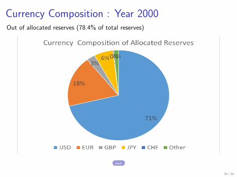
Currency Composition : Year 2000Out of allocated reserves (78.4% of total reserves)
back
34 / 34

Trade Balance : Econometric Specification
Cross Sectional Analysis
∆TradeSurplusi,T1T2 = α + DT + βNFAxR∆NFAxRi,T1T2 + βRSRV ∆RSRVi,T1T2
∆βR&KAClosedRSRVi,T1T2 × KAClosedi,T1T2 + εi
(4)
where T1T2 is period 12 and period 23, DT denotes a period fixed effect forperiod 12 and period 23 sample.
Annual Panel Analysis
log(REERit) = αi + Dt + βNFAxRNFAxRit + βRSRVRSRVit + εit
(5)
where Dt denotes a year fixed effect, and t denotes years rather than the period T.
back
34 / 34

Empirical Results : Capital Account Policy and
Trade BalanceTable 10: Trade Balances and Reserve Accumulations: Annual Panel with Fixed Effects
Period 123 (1975–2007)
Dependent variable: Full Advanced Developing Financially FinanciallyNet Exports Sample Countries Countries Open Closed
(1) (2) (3) (4) (5)
NFAxR 0.00 0.06∗ -0.01 0.01 -0.00(0.22) (2.01) (-0.42) (0.30) (-0.12)
RSRV 0.16∗∗ -0.25 0.20∗∗ 0.11 0.24∗∗
(2.16) (-1.40) (2.61) (1.03) (2.21)
Observations 2379 705 1674 1211 1168Countries 75 22 53 38 37R2 0.08 0.30 0.09 0.08 0.10
p-value: βNFAxR 6= βRSRV 0.06 0.12 0.02 0.41 0.05
back
34 / 34

Capital Account Policy - RSRV and KAControl
Scatter-plot : Period3 1997-2007
USA3GBR3 AUT3
BEL3
DNK3FRA3DEU3ITA3NLD3 SWE3 CHE3CAN3 JPN3FIN3
GRC3
ISL3
IRL3PRT3ESP3
TUR3
AUS3
NZL3
ARG3
BOL3
BRA3
CHL3
COL3
CRI3
DOM3
SLV3
GTM3
HND3
MEX3
PRY3
PER3URY3JAM3
CYP3
ISR3
JOR3
EGY3
LKA3
IND3
KOR3
MYS3
NPL3PAK3
PHL3
THA3
BDI3
CMR3
GMB3
CIV3
KEN3
MDG3
MAR3NER3 SEN3TZA3TGO3SLB3 FJI3
PNG3
CHN3
−2−1
01
2Av
erag
e C
apita
l Acc
ount
Con
trol I
ndex
0 .1 .2 .3 .4Average Reserve Accumulation (1997−2007)
back
34 / 34

Growth : Econometric Specification
Cross Sectional Analysis
∆log(yi ) = α + βRSRV ∆RSRVi + βR&KAClosed∆RSRVi × KAClosedi
+βInitialGDP log(yi,0) + γ′Zi + εi , (6)
where y is the average real GDP per capita or TFP for period 2 or 3. The initialvalue of real GDP per capita or TFP comes from the the last year of the period 1.Z stands for all other controls.
Annual Panel Analysis
log(yi,t)− log(yi,t−1) = αi + Dt + βRSRV (RSRVi,t−1 − RSRVi,t−2)
+βInitial log(yi,t−1) + γ′Zi,t + εi,t . (7)
back
34 / 34

Empirical Results : Capital Account Policy and
rGDP GrowthTable 17a: Annual Panel: Capital Account Policy and Growth of Real GDP per Capita
Period 2 & Period 3 (1986-2007)
Dependent variable: All Sample
rGDP Growth All Fin.Opn. Fin.Cl. Adv. EM Dev.
(1) (2) (3) (4) (5) (6)
Lagged ∆ RSRV 0.07 0.04 0.23∗∗ 0.01 0.19∗∗ 0.02(1.18) (0.56) (2.56) (0.06) (2.60) (0.31)
Initial rGDP -0.05∗∗ -0.09∗∗∗ -0.02 -0.08∗∗∗ -0.10∗∗∗ -0.02(-2.54) (-4.62) (-0.69) (-3.10) (-3.62) (-0.91)
Schooling 0.01 0.01∗ 0.00 0.00 0.04∗∗ 0.01(1.65) (2.00) (0.03) (1.19) (2.90) (1.02)
Inst. Quality 0.01∗∗∗ 0.01∗∗∗ 0.00 0.00∗ 0.01∗∗ 0.01∗
(2.93) (3.90) (0.81) (1.82) (2.60) (1.90)Trade Openness 0.03∗ 0.03∗∗∗ 0.04 0.02∗∗∗ -0.04 0.05
(1.69) (3.51) (1.28) (3.51) (-1.31) (1.62)Credit to GDP -0.00∗∗∗ -0.00∗∗∗ -0.00∗∗ -0.00 0.00 -0.00∗∗
(-3.80) (-3.08) (-2.16) (-1.09) (0.03) (-2.26)Terms of Trade -0.01 0.04 -0.04∗ 0.03 -0.11∗∗∗ 0.04∗
(-0.42) (1.36) (-2.05) (0.55) (-10.11) (1.85)
Obs. 1231 724 507 424 248 559Num. of Cty. 64 38 26 22 13 29R2 0.18 0.26 0.22 0.44 0.63 0.20
back
34 / 34

Empirical Results : Capital Account Policy and
rGDP Growth w/o OilTable 17b: Annual Panel: Capital Account Policy and Growth of Real GDP per Capita
Period 2 & Period 3 (1986-2007)
Dependent variable: w/o Oil Exporting Countries
rGDP Growth All Fin.Opn. Fin.Cl. Adv. EM Dev.
(1) (2) (3) (4) (5) (6)
Lagged ∆ RSRV 0.03 -0.05 0.23∗∗ -0.06 0.27∗∗∗ -0.03(0.38) (-0.49) (2.51) (-0.57) (3.18) (-0.26)
Initial rGDP -0.09∗∗∗ -0.11∗∗∗ -0.08∗∗∗ -0.09∗∗∗ -0.10∗∗∗ -0.08∗∗∗
(-6.72) (-4.86) (-5.28) (-3.41) (-3.39) (-3.69)Schooling 0.01∗∗ 0.01∗∗ 0.02∗ 0.00 0.04∗∗ 0.01
(2.30) (2.11) (1.84) (0.89) (2.54) (1.33)Inst. Quality 0.01∗∗∗ 0.00∗∗∗ 0.01∗∗ 0.00∗ 0.00 0.01∗
(3.30) (2.81) (2.52) (1.99) (1.38) (1.98)Trade Openness 0.01∗ 0.03∗∗∗ -0.03 0.02∗∗∗ -0.06∗ -0.02
(1.75) (3.08) (-0.91) (2.88) (-1.85) (-0.63)Credit to GDP -0.00∗∗∗ -0.00∗∗ -0.00 -0.00 -0.00 -0.00
(-3.20) (-2.49) (-1.60) (-0.57) (-0.11) (-1.35)Terms of Trade -0.04 -0.02 -0.05∗ -0.03 -0.11∗∗∗ 0.01
(-1.67) (-0.67) (-1.90) (-0.99) (-10.45) (0.51)
Obs. 1037 609 428 405 208 424Num. of Cty. 54 32 22 21 11 22R2 0.24 0.27 0.32 0.48 0.66 0.23
back
34 / 34
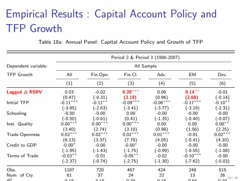
Empirical Results : Capital Account Policy and
TFP GrowthTable 18a: Annual Panel: Capital Account Policy and Growth of TFP
Period 2 & Period 3 (1986-2007)
Dependent variable: All Sample
TFP Growth All Fin.Opn. Fin.Cl. Adv. EM Dev.
(1) (2) (3) (4) (5) (6)
Lagged ∆ RSRV 0.03 -0.02 0.20∗∗∗ 0.06 0.14∗∗ -0.01(0.47) (-0.31) (3.19) (0.96) (2.60) (-0.14)
Initial TFP -0.11∗∗∗ -0.11∗∗ -0.09∗∗∗ -0.06∗∗∗ -0.17∗∗∗ -0.10∗∗
(-3.95) (-2.63) (-3.41) (-3.77) (-3.19) (-2.31)Schooling -0.00 -0.00 0.00 -0.00 -0.00 -0.00
(-0.50) (-0.61) (0.41) (-1.35) (-0.40) (-0.07)Inst. Quality 0.00∗∗∗ 0.00∗∗∗ 0.00∗∗∗ 0.00 0.00 0.00∗∗
(3.40) (2.74) (3.10) (0.98) (1.56) (2.25)Trade Openness 0.02∗∗∗ 0.02∗∗∗ 0.02∗∗∗ 0.01∗∗∗ -0.01 0.02∗∗∗
(6.13) (3.37) (7.78) (4.05) (-0.41) (4.10)Credit to GDP -0.00∗ -0.00 -0.00∗ -0.00 -0.00 -0.00
(-1.95) (-1.43) (-1.75) (-0.99) (-0.55) (-1.08)Terms of Trade -0.03∗∗ -0.01 -0.05∗∗ -0.02 -0.10∗∗∗ -0.00
(-2.37) (-0.74) (-2.75) (-1.30) (-7.62) (-0.03)
Obs. 1187 720 467 424 248 515Num. of Cty. 61 37 24 22 13 26R2 0.18 0.15 0.30 0.18 0.56 0.19
back
34 / 34

Empirical Results : Capital Account Policy and
TFP Growth w/o OilTable 18b: Annual Panel: Capital Account Policy and Growth of TFP
Period 2 & Period 3 (1986-2007)
Dependent variable: w/o Oil Exporting Countries
TFP Growth All Fin.Opn. Fin.Cl. Adv. EM Dev.
(1) (2) (3) (4) (5) (6)
Lagged ∆ RSRV 0.07∗ 0.03 0.17∗∗∗ 0.05 0.20∗∗ 0.04(1.79) (0.64) (2.92) (0.71) (2.86) (0.92)
Initial TFP -0.11∗∗∗ -0.15∗∗∗ -0.07∗∗ -0.06∗∗∗ -0.20∗∗∗ -0.10∗∗∗
(-4.57) (-4.21) (-2.63) (-3.28) (-3.38) (-3.01)Schooling -0.00 -0.00 -0.00 -0.00 -0.00 -0.00
(-0.84) (-0.93) (-0.44) (-1.35) (-0.22) (-0.56)Inst. Quality 0.00∗∗∗ 0.00∗∗ 0.00∗∗∗ 0.00 0.00 0.00∗∗
(3.02) (2.68) (2.92) (0.59) (0.53) (2.43)Trade Openness 0.01∗∗∗ 0.02∗∗∗ 0.03 0.01∗∗∗ -0.00 0.02
(4.17) (3.27) (1.17) (4.15) (-0.27) (0.86)Credit to GDP -0.00∗∗ -0.00 -0.00∗∗ -0.00 -0.00 -0.00
(-2.20) (-1.46) (-2.17) (-1.07) (-1.28) (-1.14)Terms of Trade -0.03∗ -0.01 -0.05∗ -0.02 -0.10∗∗∗ 0.01
(-1.93) (-0.67) (-2.07) (-1.52) (-6.75) (0.67)
Obs. 1013 605 408 405 208 400Num. of Cty. 52 31 21 21 11 20R2 0.21 0.24 0.27 0.19 0.65 0.21
back
34 / 34