Master thesisData Science

Radboud University

Precipitation Nowcasting using GenerativeAdversarial Networks

Author:Koert Schreurs

Supervisor:Yuliya Shapovalova

External Supervisors (KNMI):Maurice Schmeits

Kiri Whan

Second Assessor:Tom Heskes

August 26, 2021

Abstract

Radar extrapolation-based methods and machine learning models typically produce blurryprecipitation nowcasts, which are unrealistic. To overcome these limitations, previous researchhas developed a generative adversarial network to nowcast precipitation (AENN). The AENNcombines a reconstruction loss with an adversarial loss. In this thesis we explore the use ofGANs for nowcasting precipitation in the Netherlands. We compare the AENN model to thestate-of-the-art extrapolation-based model S-PROG. Furthermore, we examine the impact ofthe adversarial loss by comparing two models with the same architecture, where one receivesan adversarial loss and the other does not. Our results show that the adversarial loss reducesthe blurriness of the nowcasts and increases the machine learning model’s performance formoderate to high rain intensities. Additionally, an extensive evaluation shows that the AENNmodel performs better at forecasting rain intensities below 2.0 mm/h than S-PROG and S-PROG performs better at predicting moderate to heavy precipitation intensities above 2.0mm/h. However, none of the models were found to be skillful at predicting moderate to heavyrainfall at a scale of 1 km at a lead time of 30 or more minutes. Further research should bedone to improve the performance of the GAN on higher precipitation intensities by using areconstruction loss that gives more weight to errors in heavy rainfall.

Acknowledgements

I would first like to thank my supervisor from Radboud University, Yuliya Shapovalova, whowas always approachable for discussions and provided valuable guidance throughout my thesis.Also, I would like to thank my supervisors from KNMI, Maurice Schmeits and Kiri Whan,for their great support. I really appreciated our weekly discussions, which were really helpfuland kept me motivated. Furthermore, I also would like to thank Hidde Leijnse (KNMI) andAart Overeem (KNMI), for their valuable insights on radar data and clutter. Further, I wishto thank Eva van der Kooij, for her help with the python Pysteps module. Additionally, Iwould like to thank my parents for their support throughout my study and my uncle, John,for reviewing my thesis on writing errors. Finally, I would like to thank my family, friendsand girlfriend for their encouragement and the much needed distractions.

1

Contents

1 Introduction 4

2 Related Work 6

3 Data 83.1 Clutter . . . . . . . . . . . . . . . . . . . . . . . . . . . . . . . . . . . . . . . . 9

4 Generative Adversarial Networks 144.1 Background . . . . . . . . . . . . . . . . . . . . . . . . . . . . . . . . . . . . . 144.2 Loss . . . . . . . . . . . . . . . . . . . . . . . . . . . . . . . . . . . . . . . . . 144.3 Preprocessing . . . . . . . . . . . . . . . . . . . . . . . . . . . . . . . . . . . . 164.4 Generator . . . . . . . . . . . . . . . . . . . . . . . . . . . . . . . . . . . . . . 164.5 Discriminator . . . . . . . . . . . . . . . . . . . . . . . . . . . . . . . . . . . . 174.6 Hyperparameter Tuning . . . . . . . . . . . . . . . . . . . . . . . . . . . . . . 174.7 Experimental Settings . . . . . . . . . . . . . . . . . . . . . . . . . . . . . . . 20

5 Baseline 225.1 Radar Extrapolation . . . . . . . . . . . . . . . . . . . . . . . . . . . . . . . . 22

5.1.1 Spectral Prognosis (S-PROG) . . . . . . . . . . . . . . . . . . . . . . . 225.2 Non-adversarial Generator (NAG) . . . . . . . . . . . . . . . . . . . . . . . . 23

6 Evaluation 246.1 Continuous Scores . . . . . . . . . . . . . . . . . . . . . . . . . . . . . . . . . 246.2 Categorical Scores . . . . . . . . . . . . . . . . . . . . . . . . . . . . . . . . . 24

6.2.1 Fractions Skill score . . . . . . . . . . . . . . . . . . . . . . . . . . . . 256.3 Train Test Split . . . . . . . . . . . . . . . . . . . . . . . . . . . . . . . . . . . 27

7 Results 287.1 Nowcasting Performance . . . . . . . . . . . . . . . . . . . . . . . . . . . . . . 287.2 Influence of Data Splitting . . . . . . . . . . . . . . . . . . . . . . . . . . . . . 317.3 Visualization of the Nowcast Methods . . . . . . . . . . . . . . . . . . . . . . 33

8 Discussion 36

9 Conclusion 40

2

A Appendix 47A.1 Clutter-removal using Gradients . . . . . . . . . . . . . . . . . . . . . . . . . 47A.2 Hyperparameter Tuning . . . . . . . . . . . . . . . . . . . . . . . . . . . . . . 50

A.2.1 Label Smoothing . . . . . . . . . . . . . . . . . . . . . . . . . . . . . . 50A.2.2 Learning Rate . . . . . . . . . . . . . . . . . . . . . . . . . . . . . . . 50

A.3 Artifact in GAN output . . . . . . . . . . . . . . . . . . . . . . . . . . . . . . 51A.4 MFBS dataset . . . . . . . . . . . . . . . . . . . . . . . . . . . . . . . . . . . 52

3

Chapter 1

Introduction

Rain has a large influence on everyday life. Reliable precipitation forecasts are essential in thedecision-making of industries such as agriculture [30], traffic [11], aviation [37] and construc-tion [53]. Precipitation nowcasting, i.e. short-term forecasts of up to 6 hours, are importantfor water-related risk management. Warning systems rely on nowcasts in order to generatea warning in time for a user to take preventative actions [58, 17]. Given that the frequencyand intensity of heavy rainfall events is expected to increase due to climate change, the needfor accurate precipitation nowcasting becomes ever more important [3].

Traditionally nowcasts are made using Numerical Weather Prediction (NWP) models orradar extrapolation-based models [5]. NWP models use physics-based models to forecastthe weather. These models require a substantial amount of computation power and theirspatial and temporal resolution is often too low for precipitation nowcasting. Extrapolation-based models, such as optical flow [10], use observations obtained by weather radars to makeforecasts. Optical flow models extrapolate by computing a motion field from past radar dataand advecting the most recent radar observations along this trajectory. Radar extrapolation-based models have a higher spatial and temporal resolution than NWP models. Optical-flowmethods are designed with the assumptions of Lagrangian persistence in mind, which assumesthat 1) the total rain intensity remains constant and 2) the motion field remains constant[19]. However, Lagrangian persistence does not always hold as the motion and intensity canvary with respect to time and thus these assumptions can hinder the model’s performance.

Recent studies have successfully applied machine learning (ML) for weather nowcasting [66,54, 61]. Machine learning methods, such as deep learning (DL), take advantage of the largeamount of available historical weather data. These models are not hindered by the assumptionof Lagrangian persistence. However, the deep learning approaches tend to result in predic-tions that are smooth/blurry and look unrealistic as result of optimizing with a standard lossfunction like mean-squared-error (MSE) [60]. A class of generative ML frameworks calledGenerative Adversarial Network (GAN) has been to shown to address this issue [26, 33, 59].Jing et al. proposed the Adversarial Extrapolation Neural Network (AENN) GAN model thatoutperformed other state-of-the-art models [33]. In the GAN framework two DL models arepitted against each other in an adversarial way. The generator generates synthetic samplesand the discriminator has to discriminate between real and synthetic samples. The genera-tive model does not train to minimize the distance to a target image, but it trains to fool

4

the discriminator. Ideally, this results in the generating learning to approximate the targetdistribution, resulting in realistic forecasts.

In this thesis, we explore the use of GANs to perform precipitation nowcasting over theNetherlands. The GAN model AENN was trained and evaluated on Dutch precipitationradar data made available by the Royal Dutch Meteorological Institute (KNMI). Addition-ally, we included a more extensive verification compared to previous studies. The GAN modelwas compared to the state-of-the-art optical flow model Spectral Prognosis (S-PROG) [52].Furthermore, we demonstrated the influence of an adversarial loss by comparing a generatortrained with adversarial loss and without it.

The remaining part of this thesis is organized as follows. In Chapter 2 further background isgiven on machine learning in weather prediction. Chapter 3 gives details about the datasetused and explains the methodology that was used to select samples from the dataset. Chapter4 provides details about the GAN model that was used in this study. Chapter 5 explains themodels that were used as a baseline for the GAN model. Chapter 6 discusses the evaluationmetrics that were used. The results are presented in Chapter 7 and discussed in Chapter 8.Chapter 9 discusses the conclusions.

5

Chapter 2

Related Work

In this Chapter we present a brief overview of related work on machine learning in weatherforecasting.

Radar extrapolation is a sequence prediction problem. Therefore, it is closely linked to re-current neural networks like long short-term memory (LSTM) [27] and gated recurrent unit(GRU) [13]. Additionally, radar echo maps can be represented as images making the taskof radar extrapolation also a computer vision problem. Therefore, the task is also linked toconvolutional neural networks (CNN) that can deal with spatial structures in the data.

Sutskever et al. proposed a general sequence-to-sequence LSTM framework for sequenceprediction [56]. Shi et al. extended this framework to deal with the radar extrapolationproblem[66]. The authors proposed a novel convolutional LSTM (ConvLSTM) model for pre-cipitation nowcasting. The sequence-to-sequence framework was extended by using multipleConvLSTM layers to create an encoding-forecasting framework. The ConvLSTM model pro-vides a framework for dealing with spatiotemporal relationships. The Critical Success Index(CSI), False Alarm Rate (FAR), Probability of Detection (POD), and correlation scores ofpredicting 0.5 mm/h rain rate threshold was used to evaluate the model. The authors showthat their model outperforms the state-of-the-art optical flow model ROVER. In a follow uppaper, Shi et al. showed that other categories of RNN, like GRU, can also be extended intoa ConvRNN framework [54]. Furthermore, the authors proposed the Trajectory GRU (Tra-jGRU) model, which improves upon ConvRNN models. Unlike the ConvRNN models, TheTrajGRU can learn location-variant structure. Additionally, they introduced Balanced MeanSquared Error (B-MSE) loss function. The B-MSE loss function penalizes errors on heavyprecipitation more, resulting in better performance on heavier precipitation. Recent work byVan der Kooij assessed the performance of the TrajGRU model in the Netherlands [61]. Theauthor showed that the TrajGRU was able to outperform the optical-flow method S-PROG.

A common downside of using deep learning approaches to forecast precipitation is that theresults look blurry and are not realistic. GAN have seen great success in generating realisticsynthetics images [21]. GANs have also been used for weather forecasting. Bihlo used an en-semble of GANs for forecasting different weather variables [9]. The predicted variables werethe geopotential height of the 500hPa pressure level, the two-meter temperature and the totalprecipitation for the next 24 hours in Europe. The GAN model was able to reach a good per-

6

formance on all variables except for total precipitation. Furthermore, Dai used an ensembleof GANs for post-processing NWP forecasts of cloud-cover [16]. The author showed that theGAN model outperformed traditional state-of-the-art port-processing models. Furthermore,the GAN’s output was less blurry and looked more realistic when compared to other deeplearning approaches.

Some notable work has also been done on nowcasting precipitation using GANs. Hay-atbini et al. proposed a conditional GAN to estimate precipitation [26]. Two models weredeveloped for this task. They first trained a model to predict a rain/no-rain binary map.Then the regression model predicts for each rainy pixel its quantity. The latter was done witha GAN network. The authors used the U-Net architecture [50] for the generator model. Theregression model uses a combination of MSE loss and adversarial loss. The proposed modelwas shown to outperform other baseline models that were trained without an adversarialloss component. Furthermore, Tian et al. propose a GAN model (GA-ConvGRU) where thegenerator uses a ConvGRU framework and the discriminator is a CNN [59]. The generatorwas trained with a loss function that combines MSE and the adversarial loss. The authorsused two years for training data and excluded images with an average rainfall rate below0.01 mm/h. The authors evaluate their model by using the metrics POD, FAR, CSI andHeidke Skill Score (HSS) [65, Chapter 8.2] in combination with thresholds of 0.5, 5, 10, and30 mm/h. The GA-ConvGRU was shown to obtain a better POD score than ConvGRU acrossall thresholds, however for the other metrics the two models performed similarly. Addition-ally, the authors showed that their GAN model yield more realistic results when compared tothe ConvGRU framework. Besides Jing et al. proposed the Adversarial Extrapolation NeuralNetwork (AENN) model, which is a GAN framework with one generator and two discrimi-nators [33]. This model improves upon the ConvLSTM framework by adding an adversarialloss to the generator. The generator creates an echo frame sequence predicting 0.5, 1 and1.5 hours ahead. The ConvLSTM framework was used for the generator part of the network.Furthermore, the AENN model consists of two discriminators. One looks at individual framesand the other looks at the sequence. For the verification metrics the authors used the POD,FAR, CSI and HSS scores with a threshold of 0.5 mm/h. The AENN model was comparedwith a state-of-the-art optical flow model and with the ConvLSTM model. The AENN modelwas able to obtain the best POD, CSI and HSS score, however the ConvLSTM was able toachieve a better FAR score. The authors showed that the output of AENN is more realisticand less blurry than the output of the ConvLSTM model.

7

Chapter 3

Data

The precipitation data that was used was collected by KNMI. KNMI has two radars, locatedin Herwijnen and Den Helder, which measure radar reflectively in dBZ every five minutes.The radar product estimates rainfall accumulation over 5 minutes by converting the dBZvalues to rain intensity by using the Z-R relationship [41]: Z = 200R1.6, where Z is the radarreflectivity factor in dB and R is the rainfall rate in mm/h. The two radars cover the Nether-lands plus areas over sea and across the Belgian and German borders.

The real-time radar product [8] is available every 5 minutes. A mean field bias correctionis applied to this data by using automatic rain gauges. From this point on we will call thisdataset the real-time (RT) dataset. An example of a few radar scans from this dataset canbe seen in Figure 3.1.

The images in the RT dataset have an image size of 765 by 700 pixels. Each pixel repre-sents a grid of 1 km by 1 km. The radar images are made at an altitude of 1.5 km. Theaccumulation values were converted to rain rates (mm/h) by multiplying the rain accumula-tion in 5 minutes by a factor of 12. The values were clipped at a maximum of 100 mm/h.Values above this are likely to be caused by hail or by echoes from sources other than pre-cipitation (i.e., clutter). This reduces the impact of false extremes, while still allowing topredict high precipitation values. Additionally, we proposed a method to reduce clutter in

Figure 3.1: Examples from the real-time radar product. The same colormap is used through-out the thesis for precipitation radar images.

8

the dataset, which is described in section 3.1. This method discards radar scans that havehigh probability of containing clutter.

Furthermore, we also discarded samples that had very low mean amounts of precipitation.Most of the time it does not rain in the Netherlands. Therefore, a large part of the dataconsists of samples without rain. The focus of this thesis lies on forecasting precipitation.Therefore, a set of rainy events was sampled from the real-time data set. We define a rainyevent as 6 consecutive 5 minute samples with rain and a radar scan was labeled as rainy if theaverage rain intensity per pixel exceeds 0.01 mm/h. A total of 41% of the data was labeled ascontaining rain. Of all 30 minute slices in the data 38% were rainy events. Figure 3.2 showsthe percentage of rainy samples per month. The pixel statistics of the rainy samples can beseen in Figure 3.4b.

Figure 3.2: Percentage of rainy samples per month

3.1 Clutter

In this section we give some background what clutter is and why it is unwanted. Further-more, we will briefly discuss the different clutter removal methods that were explored and thereason why they were not used. Lastly we introduce a method that discards samples if theyare likely to contain clutter.

Unwanted echoes can be generated by objects that are not the target of the radar. These

9

echoes are called clutter. In this project any echoes generated by things other than precipi-tation are seen as clutter. Clutter can be caused by echoes returned from the various sourceslike the ground (ground clutter), the sea (sea clutter), airplanes, birds/insects, wind turbinesor ships. Clutter can have a negative impact on the performance of the model. Furthermore,having a lot of clutter in the dataset would give an unfair advantage to a machine learningmethod as such method is able to learn to deal with clutter while an extrapolation methodcannot do this. Additionally, the clutter results in the radar overestimating the total amountof precipitation, which could be misleading when labeling samples as rainy or non-rainy.

Multiple preprocessing methods are carried out by KNMI on the raw radar data to reducethe clutter before the final radar product is realized [64, 63, 28]. However, there is still clutterin the real-time radar product. Sea clutter and moving objects like ships and wind turbineremain hard to filter out. In Figure 3.3 you can see artifacts in the sea that are caused byclutter. The figure also shows that the clutter artifacts can be relatively large, spanningmultiple pixels.

A wide range of methods can be used to remove the clutter from the precipitation radardata itself. One of the simplest methods is to create a static clutter mask that discards pixelsthat have high probability to contain clutter [34, 15, 54]. Other methods rely on the fact thatrain and clutter have a different spatial decorrelation time, in order to distinguish groundclutter [2, 55]. Other studies have used data from sources other than radar, such as satelliteimages [12, 32] and predictions from a NWP model [7, 6]. Further studies have applied ma-chine learning to distinguish precipitation from clutter [31, 24]. It was beyond this research’sscope to perform an extensive removal of clutter in the real-time radar product. Nonetheless,we explored the use of different methods for the removal of clutter, such as applying cluttermasks, removing small-scale structures, and discarding pixels with high gradients. However,removing the clutter per sample was a challenging task and no adequate simple solution forthis problem was found. In the end we did not apply any clutter removal to our dataset di-rectly, but instead we proposed a method to discard samples that are likely to contain clutter.

In order to see which areas of the radar scan tend to contain clutter, we can look at thestatistics per pixel in the dataset. In Figure 3.4a the probability of a pixel exceeding a rainintensity threshold is shown. Places that tend to contain clutter are more likely to exceedthe rain thresholds. In Figure 3.4 you can see certain spots in the sea (sea clutter) and shiptracks that often contain clutter.

10

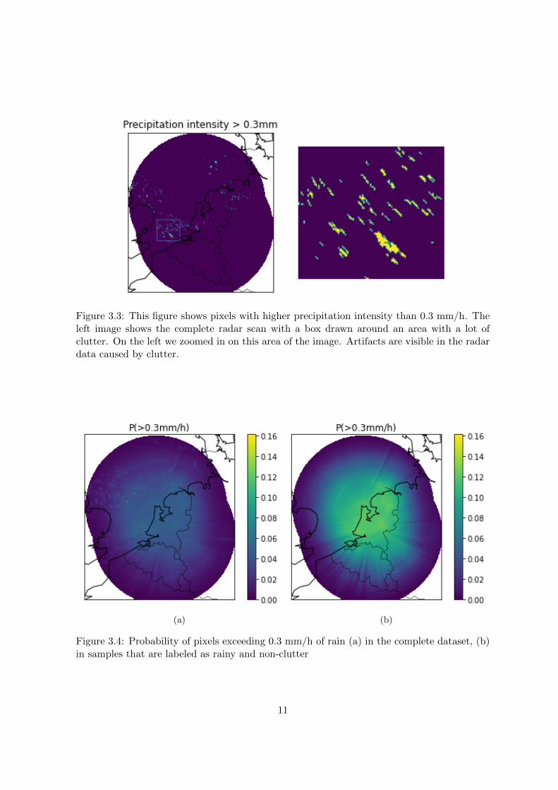
Figure 3.3: This figure shows pixels with higher precipitation intensity than 0.3 mm/h. Theleft image shows the complete radar scan with a box drawn around an area with a lot ofclutter. On the left we zoomed in on this area of the image. Artifacts are visible in the radardata caused by clutter.

(a) (b)

Figure 3.4: Probability of pixels exceeding 0.3 mm/h of rain (a) in the complete dataset, (b)in samples that are labeled as rainy and non-clutter

11

One possible method of removing clutter is to discard patches of non-zero pixels belowa certain size. Clutter artifacts often consist of only a few pixels while precipitation tendsto span larger areas. However, this method risks removing small local showers. We definea object as a cluster of 8-connected1 non-zero pixels. We can then remove objects with asize smaller than n. Choosing the right value of n is important. If n is too small, clutter isnot filtered out and if n is too big, real precipitation will be removed from the radar image.Figure 3.5 shows what happens if we remove objects that span less than 15 pixels. A lot ofthe sea clutter is removed, however removing an area of 15 km2 can also remove a lot of smallscale precipitation. Additionally, it did not remove all clutter in the images. Therefore, wedecided not to use this method of clutter removal.

Figure 3.5: Example of clutter removal by removing objects smaller than 15 pixels. Non-zeropixels are in yellow.

Another method to remove clutter is by eliminating pixels that have a high probability ofcontaining clutter. The pixel statistics reveal certain areas in the image that have a high prob-ability of containing clutter (see Figure 3.4a) By using these pixel statistics a static cluttermask can be made. However, downside of using a clutter mask is that it does not filter out allthe clutter. Not all clutter is static and can be filtered out by a clutter mask. Furthermore,the clutter mask will also filter out real precipitation. For these reasons we did not use aclutter mask in this thesis.

18-connected means a pixel has 8 neighbouring pixels. Two pixels are connected if they neighbour eachother in the horizontal, vertical or diagonal direction

12

Figure 3.6: Histogram of gradient magnitudes higher than 1 mm/h/km. A threshold was set

at a gradient magnitude of 30mm/hkm . Pixels above this threshold are seen as abnormal

Another approach that was explored was to detect clutter by looking at the gradient ofthe pixels in the radar image. Rainfall tends to gradually increase from low to high precipita-tion values, while clutter can cause sudden increases and decreases in radar reflectively, whichresults in abnormally large gradients. However, discarding pixels based on their gradientcan lead to problems when a cloud moves through areas that contain clutter or occasionallyprecipitation also contains high gradients. This makes it difficult to discard pixels based onthe magnitude of their gradient. Instead we propose to use the number of high gradients in aradar image as an indication of the amount of clutter in the radar scan. Images with a lot ofclutter can be discarded. The magnitude of the gradients was calculated by computing thegradient from left to right and top to bottom of the image and then taking the square root ofsum of squares. A histogram of gradient magnitudes is depicted in Figure 3.6. A thresholdwas set at a gradient magnitude of 30 mm/h/km. Pixels with a gradient bigger than thisthreshold are seen as abnormal. Samples with clutter can be discarded by setting anotherthreshold for the number of abnormal pixels allowed in the image and discarding radar scansthat exceed this threshold. It was empirically found that images with more than 50 abnormalpixels tend to contain clutter. Therefore, we discarded samples from the dataset if they havemore than 50 abnormal pixels. Random samples of radar scans with more and fewer than 50abnormal pixels can be seen in Appendix A.1 and A.2.

In conclusion, we reduced the amount of clutter in our dataset by discarding samples thatcontain many pixels with a high gradient. We showed that such samples often contain clutter.No further preprocessing of the data was done to remove clutter in the samples.

13

Chapter 4

Generative Adversarial Networks

4.1 Background

In the Generative adversarial Networks (GANs) framework two networks compete againsteach other [21]. The generator creates synthetic samples and the discriminator predicts ifits input comes from the training set or from the generator. The generator tries to fool thediscriminator into thinking its generated samples are real. On the other hand the goal of thediscriminator is to detect fake samples. The arms race between the two models leads to acontinuous improvement of both the discriminator and the generator. When one gets betterat its task, the other has to improve its game. Ideally after finishing training the generatorhas learned to approximate the target distribution. The discriminator can then no longerdifferentiate between the synthetic and the real samples. GANs have seen a broad rangeof applications such as text-to-image generation [67], generating artificial human faces [35]and image super-resolution [38]. Furthermore, GANs have recently been used successfully inmeteorology to forecast cloud cover [9, 16] and precipitation [26, 33, 59].

In this thesis the AENN model was trained and validated on the real-time radar product.The model receives an input of 30 minutes, consisting of 6 samples. The model is tasked withforecasting the precipitation at lead times of 30, 60 and 90 minutes. Additionally, we also ex-plored the use of machine learning for forecasting radar data that was further bias-corrected,but we failed to get reasonable results (see Appendix A.4). Given the time constraints of thisresearch, we instead focused on forecasting the real-time radar product.

4.2 Loss

The mechanisms of the GAN framework proposed by Goodfellow et al. can be described inthe following way [21]. Let D be the discriminator and G be the generator. The discrimi-nator D receives an input tensor and classifies whether it comes from the real distributionpr or from the generator pg. The generator G receives random noise z ∼ pz(z) as input andfinds a mapping that maximizes the probability of D labeling the generated image G(z) asreal, Ez∼pz [logD(G(z))]. The objective of the discriminator is to maximize its output on thereal samples x, Ex∼pr [logD(x)] and minimize its output for fake samples, Ez∼pz [logD(G(z))].Minimizing Ez∼pz [logD(G(z))] is the same as maximizing Ez∼pz [log((1−D(G(z))]. By com-bining these formula the GANs loss function can be written as a minimax game between G

14

and D:minG

maxD

V (D,G) = Ex∼pr [logD(x)] + Ez∼pz [log(1−D(G(z)))] (4.1)

GANs are capable of generating random realistic samples from a given dataset [21]. However,in this framework there is no control over the images that are generated.In order to make a proper forecast, the GAN output should be dependent on recent obser-vations. In a conditional GAN (cGAN) this control is achieved by conditioning G and D onanother variable c [21, 43]. The conditional value function of the cGAN can be defined as:

minG

maxD

Vc(D,G) = Ex∼pr [logD(x|c)] + E[log(1−D(G(c)))] (4.2)

Another method to make the GAN’s output conditional is to give the generator the addi-tional task to minimize the distance between G(c) and the target value y. This results inthe output having to match two criteria: 1) the nowcast should match the ground-truth asclose as possible, this is measured with the reconstruction loss (e.g. MSE or MAE). 2) thenowcast should also fool the discriminator into thinking the generated samples are real, thisis measured with the adversarial loss. Recent work on radar extrapolation using GANs haveused this approach either in combination with a cGAN [26, 33] or with just a GAN model[59]. As reconstruction loss, lrec, Jing et al. used the sum of the MSE and the MAE for theAENN’s generator model [33].

MSE =1

N

N∑n=1

3∑t=1

765∑i=1

700∑j=1

(yn,t(i, j)− xn,t(i, j))2 (4.3)

MAE =1

N

N∑n=1

3∑t=1

765∑i=1

700∑j=1

|yn,t(i, j)− xn,t(i, j)| (4.4)

where N is the number of samples, t is the lead time, yn is the target value of sample n, xnis the predicted value of n and i and j are the row and column index of the pixel. It wasempirically found that the model was more stable when only using the MSE as reconstructionloss, Lrec = Lmse. We speculate that the reason for this is that the MAE gives relatively moreweight to small mistakes. The radar scans in general contain a lot of pixels with no rain, thesepixels have a value of exactly 0. Being slightly off on a lot of these pixels significantly lowersthe MAE. The MSE is less sensitive to this. The AENN generator uses a ReLU activation[44] in its final layer that sets negative values to 0. A strategy to get a low MAE would beto make sure the network’s output is always negative. Then the ReLU activation causes theoutput of the network to become exactly 0, resulting in a lower MAE score. However, theReLU has gradient of 0 for negative values. Therefore, the model cannot use gradient descentto get out of this local minimum and gets stuck during training.

In the AENN model there are two discriminators:

1. The frame discriminator, Dfra, judges each individual frame independently. The objec-tive function of the frame discriminator, Lfra, is to maximize for time t the sum overn ∈ (6, 12, 18)1 in Eq. 4.1, with x = xt+n and G receives as input c = (xt−5, xt−4, xt−3, xt−2, xt−1, xt)instead of noise variable z.

1Note that the interval between samples is 5 min., so the lead times of 30, 60 and 90 min. correspond tothe samples t+ 6, t+ 12 and t+ 18, respectively

15

2. The sequence discriminator, Dseq, is a cGAN and receives as input the sequence of ob-servations and either the target values or the predictions. The objective of the sequencediscriminator, Lseq, is to maximize Eq. 4.2 with c = (xt−5, xt−4, xt−3, xt−2, xt−1, xt) andx = (xt+6, xt+12, xt+18)

The generator tries to minimize the objective function of both discriminators. The completevalue function of the AENN model as used in this paper can be described as follows:

minG

maxDfra,Dseq

Vaenn(Dfra, Dseq, G) = λadvLfra + λadvLseq + λrecLmse (4.5)

where λadv, λrec are the weights for the adversarial loss and the reconstruction loss, respec-tively.

4.3 Preprocessing

The AENN model was designed to work with input and output image dimensions of 256 by256 pixels. To comply with this, preprocessing was done to downscale the dataset to 256 by256 pixels. In our original datasets the images have a dimension of 765 by 700. For the realtime dataset zero padding was used to make the images a square of 768 by 768. Afterward,bilinear interpolation [18] was applied in order to reduce the image size by a factor of three,making its size 256 by 256 pixels. As in the original AENN paper, we converted the rainfallrate values to dBZ values using the Z-R relationship(Z = 200R1.6) [41]. Furthermore, min-max normalization was used to normalize the values between 0 and 1. The preprocessingsteps were undone during the validation and testing of the model.

4.4 Generator

The generator receives an input sequence of past radar observations and outputs another se-quence of radar images that make up the forecast of the model. This task is called sequence tosequence prediction. The network uses an encoder-decoder architecture [56, 66]. The spatialfeatures of the input sequences are first encoded into a feature space by using multiple convo-lution layers. These layers are strided causing the dimensionality of the input to be reducedafter each layer. This encourages the model to learn a compact representation of the inputdata. The sequence of encoded images is then processed by Convolution Recurrent NeuralNetwork (ConvRNN) layers. These layers can deal with both spatial and temporal patterns inthe data. The ConvRNN forecasts encoded images. These encoded images are then decodedby the decoder part of the network that consists of strided transposed convolutional layerswhich upsample the output to the desired dimensions. In Figure 4.1 the architecture of thegenerator is depicted.

The encoder consists of 3 convolutional layers. These layers have 32, 64 and 128 filters,respectively. All layers have a stride of 2 by 2, such that after each layer the image dimen-sions are halved. The first layer has a kernel size of 5 by 5 and the other layers have akernel size of 3 by 3. In the original AENN model an ConvLSTM was used to deal withtemporal-spatial dependencies. In this project we explore the use of ConvGRU instead of aConvLSTM for this layer. Two ConvGRU layers are used, the first one encodes the spatial-temporal sequence into a feature space. The second ConvGRU unrolls this feature space into

16

a prediction. Both layers have 128 filters and a kernel size of 3 by 3. The decoder part ofthe network is the encoder in reverse. It uses 3 transposed convolutional layers with 64, 32,1 filters, respectively. All layers have a stride of 2 and a kernel size of 3. The last layer usesa Rectified Linear Unit (ReLU) activation (f(x) = max(0, x)) [44]. This prevents the modelfrom predicting negative precipitation levels. The other layers use a leaky ReLU activation,f(x) = max(αx, x), where the slope α was set to 0.2 [40]. The slope prevents the problem ofa zero-gradient that is present in the ReLU activation function. A zero-gradient can be prob-lematic as no gradient-based optimization can be performed to adjust the neurons weights.This can result in a neuron becoming inactive forever because it is only able to update itsweights when it is active.

4.5 Discriminator

The AENN uses two discriminators. One only looks at a single frame and the other looks atthe complete sequence. The generator tries to create both a realistic image as well as a realis-tic sequence. The two discriminators share the same network architecture. The architectureof the discriminator is visualized in Figure 4.2.

The discriminator consists of 5 convolutional layers. These layers have 32, 64, 128, 256 and512 filters, respectively. A kernel size of 3 by 3 is used except for the first layer which has akernel size of 5 by 5. Each layer has a stride of 2 by 2. The last convolutional layer is followedby an average pooling layer which is then followed by a dense layer with 1 output. The lastlayer uses a sigmoid activation function. The other layers use a leaky ReLU activation with aslope of 0.2. The frame discriminator receives an input of length 1 is provided, which is eitherthe prediction or the target at a lead time 30, 60 or 90 minutes. The sequence discriminatorreceives an input of length 9, which consists of half an hour of observations together with theforecasts or targets at the three lead times.

4.6 Hyperparameter Tuning

Various tests were done in order to find optimal parameter settings for the AENN model.Because of time constraints no extensive hyperparameter search was done, therefore the finalhyperparameter setting is likely not the most optimal. We iteratively changed hyperparame-ters of the AENN model to see if it improved the model’s results on the validation set. Thehyperparameter setting that obtained the highest performance on the validation set was kept.

Neural network classifiers can be prone to producing extremely confident predictions, es-pecially when the input is constructed in an adversarial manner [22]. This is not good forregularization. A technique called label smoothing can be used to counteract this. Labelsmoothing has been shown to improve stability and training of GAN models [51, 57]. Wecan apply label smoothing to the GAN by providing the discriminator with smoothed targetssuch as 0.1 and 0.9 instead of 0 and 1. The target label y can be smoothed with the formula:

y ∗ (1.0− α) + 0.5 ∗ α (4.6)

where α controls the amount of smoothing, when α is 0 no smoothing occurs. We comparedthe effect of label smoothing (α = 0.2) versus no label smoothing (α = 0). It was found that

17

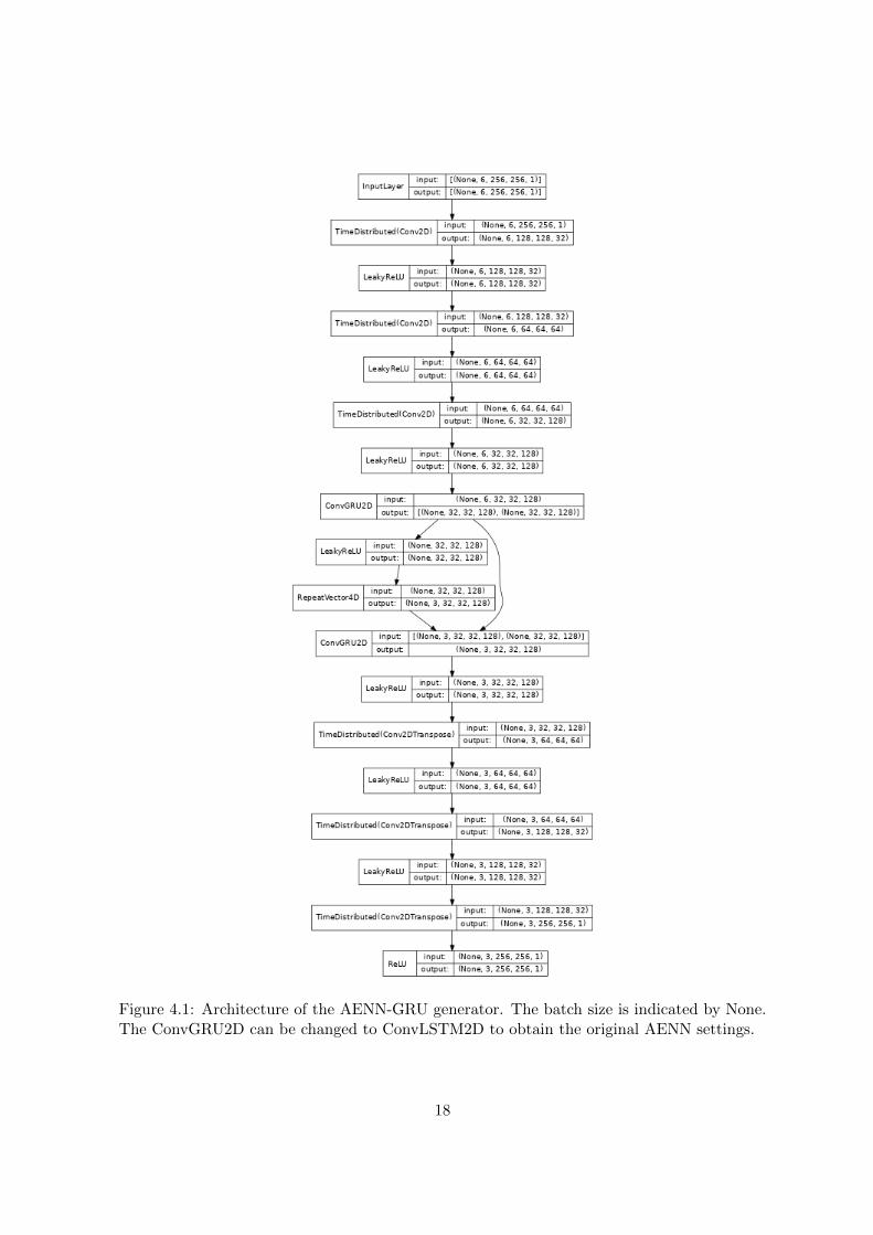
Figure 4.1: Architecture of the AENN-GRU generator. The batch size is indicated by None.The ConvGRU2D can be changed to ConvLSTM2D to obtain the original AENN settings.

18

Figure 4.2: Architecture of the sequence discriminator. The frame discriminator has the samearchitecture except the input sequence length is 1 instead of 9. The batch size is indicatedby None.

19

CSI MSE

Threshold (mm/h) Lead times(min.)

0 0.5 5 10 30 30 60 90

S-PROG 0.487 0.346 0.094 0.033 0.001 0.182 0.223 0.264

AENN 0.461 0.353 0.047 0.010 0.000 0.143 0.170 0.195

AENN-ConvGRU 0.491 0.343 0.070 0.016 0.000 0.150 0.190 0.213

Table 4.1: Comparison between AENN, AENN-ConvGRU and the S-PROG baseline in termsof CSI across all lead times per rain threshold in mm/h (higher is better) and MSE per leadtime in minutes (lower is better). The best result is indicated in bold and the second bestresult is underlined.

smoothing the labels of the discriminator slightly improved the GAN’s validation performance(see Appendix A.3) . Therefore, from this point on label smoothing with an α of 0.2 wasapplied to the AENN model.

Additionally, we compared the performance of the AENN model with different ConvRNNlayers. The AENN model uses ConvLSTM for the ConvRNN layers. However, recent studieshave explored the use of ConvGRU layers in precipitation nowcasting [54, 59]. We comparedthe AENN model with ConvLSTM layers (AENN) versus the AENN model with ConvGRUlayers (AENN-ConvGRU). In Table 4.1 a comparison between AENN and AENN-ConvGRUand the baseline S-PROG is depicted. The CSI scores were computed across all lead times. Itwas found that the AENN had a lower MSE on the validation dataset. However, the CSI scoresreveal that the AENN-ConvGRU is better at predicting precipitation of intensities above 5.0mm/h. Given that correctly predicting higher levels of precipitation is more important to us,we opted to use the AENN-ConvGRU model from this point on.

Lastly we experimented with using different learning rates for the generator and discrim-inator of the AENN model. The learning rates that were considered were: 1× 10−4, 5× 10−5

and 1× 10−5 . It was found that lowering the learning rate did not improve performance ofthe AENN model (see Appendix A.4). Therefore, we kept the learning rate at its originalvalue of 1× 10−4.

4.7 Experimental Settings

The model was implemented in python using the Tensorflow Keras library [1]. The codeis available on Github2. The weights of the neurons were set by using the Glorot uniforminitialization [20] with 0 bias. The weight of the reconstruction loss, λrec, was set to 1 and theweight of the adversarial loss, λadv, was set to 0.003 as proposed in the original AENN paper.Both the generator and the discriminators use an Adam optimizer [36] with learning rate of0.0001. ConvGRU was used for the ConvRNN part of the AENN model. Furthermore, thegenerator was trained 3 times for every update step of the discriminator. The best model interms of validation reconstruction loss was selected after 100 epochs with early stopping after20 epochs of seeing no improvements, in terms of validation reconstruction loss. The batch

2https://github.com/KoertS/precipitation-nowcasting-using-GANs

20

size was set to 16, which was the largest possible value that could fit in memory. From nowon, we will simply refer to this model with these settings as the GAN model.

21

Chapter 5

Baseline

The performance of the GAN was compared with two other models. The radar extrapolation-based model S-PROG [23] serves as a baseline for the GAN. Furthermore, we compared theGAN generator with a generator that was trained without adversarial loss, in order to assessthe improvements that the adversarial loss provides.

5.1 Radar Extrapolation

Extrapolation-based models make predictions by moving the precipitation along its mostrecent direction with its most recent speed. The trajectory is derived from recent observations.Unlike the GAN model these models do not need training. In order to make an extrapolation-based forecast the following two steps need to be performed:

1. First a motion field has to be computed based upon recent observations.

2. Secondly, the motion field is used to move the precipitation along its current trajectory.

These steps come from the assumption of Lagrangian persistence [19]. This assumption entailsthat the precipitation will move with the same speed in the same direction over the course ofthe forecasting period.

5.1.1 Spectral Prognosis (S-PROG)

Research has shown that the lifetime of precipitation is dependent on its spatial scale [62, 23].Large-scale rain features generally have a longer lifetime than small-scale rain features. Seedproposed the Spectral Prognosis (S-PROG) model [52]. This extrapolation-based model han-dles different scales of precipitation in different ways. S-PROG decomposes the precipitationfield into a multiplicative cascade. The different levels of the cascade represent different scalerain features.

An implementation of the S-PROG algorithm is available in the Python library [47]. Pystepsis an open-source library for precipitation nowcasting. Imhoff et al. compared multiple open-source precipitation nowcasting algorithms with each other [29]. The algorithms that werecompared are: Rainymotion Sparse, Rainymotion DenseRotation, Pysteps deterministic (S-PROG) and Pysteps probabilistic (STEPS) with 20 ensemble members. The authors foundthat Pysteps deterministic had the longest average decorrelation times. Furthermore, they

22

showed that in general the two Pysteps algorithms outperform the Rainymotion algorithms.The authors speculate that most errors come from the algorithms not taking into account thegrowth and dissipation processes. In this study we used the same S-PROG setup as in Imhoffet al.. The setup consists of the following steps. First, the rain rates were converted to dBZvalues. After that, the motion field was determined by using a dense Lucas-Kanade opticalflow method [39]. Semi-Lagrangian backward extrapolation was applied to the reflectivityfield. The order of the autoregressive model was set to 2 and eight cascade levels were used.With a probability matching method, the statistics of the forecast are matched with those ofthe observations based on the mean of the observations. Lastly the forecast was transformedback from dBZ to rain rate (mm/h).

5.2 Non-adversarial Generator (NAG)

The adversarial loss forces the GAN model to make predictions that look like the real data.If we leave this adversarial loss, this restriction is left out. To examine the influence ofthe adversarial loss, we implemented a non-adversarial generator (NAG). The NAG sharesthe exact same architecture as the GAN’s generator. Furthermore, we used the exact samesettings for the NAG model as for the GAN model. The only difference is that the NAG’sloss function consists of only the MSE component without any adversarial loss. The weightof the adversarial loss, λadv, was set to 0. The expectation is that this model will outperformthe GAN model in terms of MSE, as its only objective is to minimize this score. However,we also expect that the predictions of NAG will look smoother and more unrealistic than theGAN’s predictions because the NAG does not have an adversarial loss.

23

Chapter 6

Evaluation

Before we can compare models to the target values, we need to apply some post processing tothe machine learning models’ output. The predictions are denormalized and then convertedback from dBZ to rainfall rate by using the Z-R relationship (Z = 200R1.6) [41]. We evaluatethe model on the original image with size of 765 by 700. The model output’s is of size 256 by256, so in order to compute the metrics we need to upsample the output. We used bilinearinterpolation to upsample the model’s output to a size of 768 by 768 (factor of 3). Then weapplied cropping to get to the dimensions of 765 by 700.

A number of different metrics were used in order to evaluate the model and the baselinemethods. The metrics can be divided into continuous scores and categorical scores.

6.1 Continuous Scores

The two continuous score metrics that were considered are the Mean Squared Error (MSE)and the Mean Absolute Error (MAE). The metrics are calculated for the lead times 30, 60and 90 minutes. The MSE and MAE are defined as follows:

MSE =1

N

N∑n=1

765∑i=1

700∑j=1

(yn(i, j)− xn(i, j))2

(6.1)

MAE =1

N

N∑n=1

765∑i=1

700∑j=1

|yn(i, j)− xn(i, j)|

(6.2)

where N is the number of samples, yn is the target value of sample n, xn is the predictedvalue of n and i and j are the row and column index of the pixel.

6.2 Categorical Scores

The categorical scores show the performance of the model on different levels of rain intensity.The scores can be computed by converting the target and the predictions to binary images bysetting a rain threshold. To see the model performance on different rain intensities, we used 7different rainfall rate thresholds. The thresholds used are: 0., 0.5, 1.0, 2.0, 5.0, 10.0 and 30.0mm/h. Pixels above the threshold are labeled as 1 and pixels below are labeled as 0. Thisallows us to compute a confusion matrix (also known as a contingency table; see Table 6.1).

24

Predicted Positive Predicted Negative

Actual Positive True Positive (TP) False Negative (FN)

Actual Negative False Positive (FP) True Negative (TN)

Table 6.1: Confusion Matrix

By using this matrix we calculate various verification scores that are commonly used inmeteorology. The scores that are used are the Probability of Detection (POD; also calledrecall), the Critical Success Index (CSI), the False Alarm Ratio (FAR) and the bias (for moreinformation see [65, Chapter 8.2]). These metrics are defined as follows:

POD =TP

TP + FN(6.3)

FAR =FP

TP + FP(6.4)

CSI =TP

TP + FN + FP(6.5)

bias =TP + FP

TP + FN(6.6)

The CSI (also called threat score) and the bias can be expressed in terms of POD and thesuccess ratio (SR = 1 - FAR).

CSI =1

1SR + 1

POD − 1(6.7) bias =

POD

SR(6.8)

In a performance diagram, this relation is used to visualize all 4 terms in a single plot [49].Figure 6.1 shows an example of such diagram. The x-axis is the SR (1-FAR) and the y-axisindicates the POD score. Lines are drawn to indicate different biases (dashed lines) and CSIvalues (curved lines). The optimal model would lay in the upper right corner.

6.2.1 Fractions Skill score

The Fractions Skill Score (FSS) is a spatial verification measure that assesses the performanceof forecasts on different scales for a given rain rate threshold [48]. In order to compute theFSS a window with a scale of n is moved across the image to compute the fraction of pixelsinside the window with a value of 1 (i.e., if the pixel has exceeded the threshold). This resultsin a matrix of fractions in the observed image O(n) and in the forecast image F (n). The FSSis then defined as:

FSS(n) = 1− MSE(n)

MSE(n)ref(6.9)

where MSE(n) is the MSE between O(n) and F (n) and the reference, MSE(n)ref , is thelargest possible MSE between the observation and the forecast:

MSE(n)ref =1

NxNy

Nx∑i=1

Ny∑j=1

O(n)2i,j +

Nx∑i=1

Ny∑j=1

F (n)2i,j

(6.10)

where Nx and Ny are the number of rows and columns in the radar data and i and j indicatethe row and column index of the fraction matrices, respectively.

25

Figure 6.1: This figure shows a performance diagram. The SR and POD are plotted on the x-and y-axis, respectively. The dashed line shows the bias frequencies and the solid lines showsthe CSI scores.

26

Dataset Period Nr. Sequences

Training 2008-01-01 till 2018-12-31 67105

Validation 2019-01-01 till 2019-12-31 6570

Testing 2020-01-01 till 2020-12-31 6324

Table 6.2: Dataset for training, validation and testing

Dataset Period Nr. Sequences

Training 2008-01-01 till 2020-12-31 67105

Testing 2008-01-01 till 2020-12-31 6324

Table 6.3: Randomly split dataset for training and testing. The training and testing sampleswere randomly selected without replacement.

The FSS can range from 0 to 1, with 1 being a perfect forecast. As the scale increasesthe FSS generally increases as well. A model is seen as skillful at lead time t if its FSS scoreat t is higher than the skill of a random forecast, FSSrandom = 0.5 + f0

2 , where f0 is thewindow size divided by the size of the domain. The FSS score allows us to determine for eachmodel the maximum skillful lead time at different scales for different rain intensity thresholds.

6.3 Train Test Split

The authors of the AENN model randomly split their data into a training, validation andtest set. However, as we are dealing with time series data, splitting the data at random canbe problematic. When the model is trained using data that is not available in a real scenario,data leakage occurs. Realistically, the model cannot have seen future data, therefore its vali-dation when data leakage is present will overestimate its performance in a real-world scenario.For the purpose of preventing data leakage, we separated the dataset chronologically. Thefirst 11 years of the dataset were used for training. The most recent available year (2020) wasused as a testing set and the year before that as a validation set. The number of rain eventsper set can be seen in Table 6.2

Furthermore, we compare the performance when using random splitting instead of chrono-logical splitting to emphasize the importance of splitting time series data correctly. Theexpectation is that randomly splitting will result in data leakage, which will result in themodel obtaining a better score on its test set than a model that was trained and tested onchronologically split data. We randomly selected the same number of training and testingsamples for the randomly split dataset (Table 6.3) as we did for the chronologically splitdataset.

27

Chapter 7

Results

In this chapter we present the experimental results. In particular, we compare the forecastingperformance of the proposed GAN model versus the baseline model S-PROG and the non-adversarial neural network (NAG). Additionally, we investigate how splitting the data forcross-validation affects the forecasting performance of the GAN model. Furthermore, weshow some examples of nowcasts made by the different models to illustrate their differences.All results shown in this chapter are for nowcasts made on the independent test set. No morechanges were made to the model from this point on.

7.1 Nowcasting Performance

In this section we compare the performance of the GAN with the baseline models S-PROGand NAG in terms of forecasting performance. Performance was measured with continuousscores, MSE and MAE, as well as with the categorical scores CSI, FAR, POD and bias. Fur-thermore, we show the MSE and MAE by location on the radar map to visualize where themodels makes errors. Lastly, we computed the fractions skill score to obtain the maximumskillful lead times for forecasting different rain intensities at various scales.

Figure 7.1 shows the performance of all models in terms of their MSE and MAE for dif-ferent lead times. The S-PROG model obtained the worst MSE and MAE scores on allthresholds. The NAG model performed the best out of all three models at all lead times,followed by the GAN model.

Furthermore, we visualize the MSE and MAE per location for the different models. Thiscan be seen in Figure 7.2a. In order to better show the complete error landscape the colorbarwas set to range from 0 to the 99.9 percentile of the MSE or MAE across all models. Theoutliers are seen as bright yellow dots in this figure. This shows that there is still some clutterin the data and that all the models have trouble dealing with this. Furthermore, all modelsshow a greater average error near the radars in Herwijnen and Den Helder.

The differences in MSE and MAE per location is shown in Figure 7.2b. Here the color-bar shows the range from the 0.1 percentile till the 99.9 percentile of the MSE or MAE ofthe models. The MAE pattern of the GAN shows that the model tends to wrongly predictprecipitation in the lower right corner of the image, which is also visible in Figure 7.2a. Fur-thermore, a grid pattern of dots is visible where the model performance worse than in therest of the image. Furthermore, an area in the top left corner is visible where the ML models

28

(a) (b)

Figure 7.1: Performance of the models (S-PROG, GAN, NAG) measured with continuousscores in mm/h (a) mean squared error, (b) mean absolute error

CSI Threshold (mm/h) 0.0 0.5 1.0 2.0 5.0 10.0 30.0

S-PROG 0.487 0.350 0.280 0.189 0.073 0.022 0.003

GAN 0.494 0.354 0.283 0.182 0.054 0.011 0.000

NAG 0.302 0.363 0.263 0.137 0.022 0.001 0.000

Table 7.1: CSI scores of the different models on different precipitation rate thresholds. Thebest results are indicated in bold, the second best results are underlined.

outperform S-PROG.

Furthermore, Table 7.1 shows the CSI score of the models for different thresholds of pre-cipitation. A higher CSI score means a better performance. The GAN model performed beston predicting rain versus no rain (threshold of 0.0 mm/h). For a threshold of 0.5 mm/hthe NAG model obtained the best result and S-PROG performed the worst. However, theS-PROG model performed the best on predicting higher rain intensities equal to or above 2.0mm/h. The GAN model outperforms the NAG model on all precipitation thresholds except0.5 mm/h.

Additionally, in Figure 7.3 performance diagrams show the POD, SR, CSI and bias ofthe models at different thresholds and lead times. The rain rate thresholds of 10.0 mm/hand 30.0 mm/h were excluded as none of the models are skillful at predicting those and thePOD and SR are close to 0 for those thresholds. The further to the right the higher thesuccess ratio of the model and the further to the top the higher the POD. Deviations fromthe diagonal indicate the bias of the model. A model has a positive bias when it is above thediagonal and a negative bias if it is below the diagonal (see Chapter 6 for more information).In this diagram the model closest to the top right corner can be seen as the best model.The diagrams show that rainfall intensities of 0.5 mm/h or higher are underestimated by themodels and this bias becomes larger as the rain threshold increases.

29

(a)

(b)

Figure 7.2: (a) MSE (upper row) and MAE (lower row) per location, (b) Difference in MSE(upper row) and MAE (lower row) between GAN and S-PROG (left column) and NAG andS-PROG (right column)

30

Figure 7.3: Performance diagrams for different thresholds. S-PROG is depicted by triangles,the GAN model by circles and the NAG model by squares. The colors indicate different leadtimes ( red = 30min., blue = 60min., black = 90min.)

Lastly, the FSS was computed for the scales of 1, 3, 5, 17, 33 and 65 km, for the threedifferent lead times and on rain intensity thresholds of 0.0, 0.5, 1.0, 2.0, 5.0, 10.0 and 30.0mm/h. The maximum skillful lead time of a model for each scale and intensity is the highestlead time that reaches a skillful forecast (FSS > 0.5 + f0

2 ; subsection 6.2.1). Figure 7.4ashows the maximum skillful lead times of the baseline S-PROG model. Figure 7.4b and7.4c respectively show the difference in maximum lead times between S-PROG and GANand S-PROG and NAG. None of the models are skillful at predicting 10 or 30 mm/h at theconsidered lead times of 30 min. and higher. Rain intensities of 2.0 mm/h and 5.0 mm/h areonly possible to be skillfully predicted at a lead time of ≥ 30 min. on a scale of ≥ 2 km and≥ 16 km, respectively. The GAN model increases the maximum skillful lead times, comparedto S-PROG, of predicting 0.5 mm/h on a scale of 5 km, 1.0 mm/h on the scale of 5, 17 and33 km and also increase the skillful lead time on 2.0 mm/h on scales of 17 and 65 km by 30minutes. However, its maximum lead time decreases by 30 minutes, relatively to S-PROG,in predicting rain thresholds of 5.0 mm/h on a scale of 16 km. The skillful lead time of theNAG model is 30 minutes lower than S-PROG when predicting rain rates of 2.0 mm/h onscales of 3, 33 and 65 km, and when forecasting rain rates of 5.0 mm/h on scales of 17, 33and 65 km.

7.2 Influence of Data Splitting

In this section we discuss the influence of splitting the data into training, validation andtesting sets at random or chronologically. In the original AENN paper [33] the model wastrained and tested on a random split of training and testing data. However, this leads to

31

(a) (b) (c)

Figure 7.4: A model is seen as skillful at lead time t if the FSS score is higher than 0.5 + f02

(subsection 6.2.1)(a) Maximum skillful lead time S-PROG, (b) Difference in skillful lead times between GANand S-PROG, (c) Difference in skillful lead times between NAG and S-PROG

an unrealistic situation. The model’s training set contains information about future samplesrelative to the samples in the test set. In a real-world scenario the model would not have anyinformation about future samples. This phenomenon is called data leakage (see Chapter 6.3).In order to make a realistic training situation, we split the dataset across time. In this sectionwe compare the results for the model trained on randomly split data versus the model trainedon chronologically split data. Figure 7.5 compares the performance of a model trained on arandomly split training-testing data (GAN Random Split) versus the GAN model that wastrained on chronologically split data (GAN). No significant difference in performance betweenthe random splitting and the chronological splitting method. The two models obtain a similarperformance in terms of MAE on a lead time of 30 and 90 minutes and in terms of MSE onlead time of 30 minutes. Furthermore, the GAN Random Split performs worse in terms ofMSE on lead times of 60 and 90 minutes, and the GAN performs worse in terms of MAE ona lead time of 60 minutes.

(a) (b)

Figure 7.5: Performance of the GAN trained and tested on the chronologically splitdataset(GAN) versus when trained on randomly split training and testing set(GAN Ran-dom Split), (a) mean squared error, (b) mean absolute error

32

7.3 Visualization of the Nowcast Methods

In this section we give some examples of nowcasts made by the different models. The S-PROG and NAG model both show signs of blurring especially for later lead times of 60 and90 minutes. The GAN model does not seem to produce blurry predictions. However, at leadtimes of 60 and 90 minutes the GAN starts to wrongly forecast precipitation in the lower rightcorner of the image. The visualization of the MAE per location in Figure 7.2 also showedthat the GAN tends to make mistakes in this area.

33

Figure 7.6: Example of nowcasts made by the 3 different models for a rainy event that initiatesat 2020-02-16 19:00-19:30. The target images and the predictions are shown for the lead times30, 60 and 90 minutes (20:00, 20:30 and 21:00, respectively)

34

Figure 7.7: Example of nowcasts made by the 3 different models for a rainy event that initiatesat 2020-06-27 15:00-15:30. The target images and the predictions are shown for the lead times30, 60 and 90 minutes (16:00, 16:30 and 17:00, respectively)

35

Chapter 8

Discussion

Our results showed that the machine learning GAN model scores higher on predicting lightrain (≤2.0 mm/h) in terms of the CSI score for the lead times of 60 and 90 minutes. Thisis consistent with the work of Jing et al. [33] who also showed that the AENN GAN modeloutperformed traditional extrapolation methods when evaluating on a threshold of 0.5 mm/h.However, a more extensive evaluation showed that the baseline optical flow model S-PROGperforms better than the ML methods on predicting heavier precipitation of more than 2.0mm/h, while Jing et al. only tested the nowcasting performance at 0.5 mm/h. Given thatheavier rainfall has a bigger impact and is more dangerous than lighter rain, it is importantto take into consideration metrics that measure the model’s performances at higher rain ratethresholds. Though the AENN model does not perform well on predicting rain intensitiesabove 2.0 mm/h, we also showed that even a state-of-the-art radar extrapolation methodcannot skillfully predict such high rain intensities at a scale of 1 km at lead times of 30 min-utes or more. This goes to show how difficult this task is. However, the ConvGRU GANmodel (GA-ConvGRU) proposed in [59] was reported to outperform an optical-flow basedbaseline method for the higher rain intensities. The GA-ConvGRU has over 20 million train-able parameters while the AENN model has close to 2 million trainable parameters. Theincreased capacity of the GA-ConvGRU might be an explanation for the better performanceat higher precipitation thresholds. Future work needs to be done to investigate if increasingthe model’s capacity improves forecasts of heavier precipitation.

Furthermore, Figure 7.1 showed that the two machine learning models, GAN and NAG,both outperformed the optical flow model S-PROG in terms of MSE and MAE. However, thelow MSE and MAE of the ML models are likely explained by their ability to predict lightrain (≤2.0 mm/h), which is much more common than the heavier precipitation intensities.On the basis of MSE and MAE, the S-PROG performance is the worst. However, the CSIscores reveal that the S-PROG algorithm is better at predicting moderate to high intensityprecipitation. The continuous scores do not provide a complete picture of the performanceof a precipitation nowcasting model, so it is vital to evaluate such model with multiple met-rics. Furthermore, these findings also show the downsides of using MSE as a loss functionfor precipitation nowcasting. Optimizing for MSE leads to the model only learning to predictlight precipitation well, while in a real-world scenario the ability to forecast heavy rain inten-sities is important. We showed that the adversarial loss improves the forecasts of higher rainintensities which is consistent with the work in [26]. Another study proposed the balanced

36

MSE (B-MSE) and balanced MAE (B-MAE) as a loss function for precipitation nowcasting[54]. In the B-MSE and B-MAE more weight is assigned to heavier precipitation during thecalculation of the MSE and MAE. The balanced MSE (B-MSE) and balanced MAE (B-MAE)was reported to increase the model’s performance on predicting heavier rainfall.

Furthermore, the visualization of forecasts of the different models (Chapter 7.3) demon-strated that a model trained on only MSE (i.e. NAG) showed blurry forecasts which areunrealistic. This is also the case for extrapolation-based models like S-PROG. The predic-tions of the GAN model were not blurry.

In summary, we can conclude that the MSE does not seem to correlate well with humanjudgement of what makes good forecasts. Our findings are in line with previous researchthat showed that optimizing for a low MSE results in blurry output [42] and a bias towardspredicting low rain intensity thresholds [54]. The adversarial loss was shown to help withboth of these problems. Further research on precipitation nowcasting should try to avoidoptimizing MSE and instead use a loss that encourages the model to learn to predict higherrain intensities better, like for example the B-MSE [54].

Visualization of the average error per pixel revealed that there are some strange artifactspresent in the output of the GAN model (see Figure 7.2). Firstly, Figure 7.2b showed thatthe errors of the GAN form a repeated pattern like a grid. We do not know for sure whatcaused this. We speculate that these artifacts are caused by the transposed convolution lay-ers. Studies have reported that these can cause a checkerboard like pattern to emerge inthe neural network’s output [45]. Applying bilinear interpolation upscaling to this patternmight transform the checkerboard artifacts into the form of a grid. The generator with noadversarial loss did not show this pattern. However, it is possible for a neural network tolearn to adjust its weight in order to avoid the checkerboard artifact [45]. We suspect theGAN model was not able to learn to do this. Resize-convolution layers have been shown toeliminate checkerboard artifacts [45]. Further research needs to be done to see if the grid likeerror pattern of the GAN disappears if resize-convolution layers are used instead of transposedconvolution layers.

Secondly, the MAE pattern of the GAN model (Figure 7.2a) showed an area in the bot-tom right corner where the GAN tends to make mistakes. A closer inspection of the GANnowcasts (Figure 7.6 and Figure 7.7) shows that the GAN predicted the same precipitationfield in this area for lead times of 60 and 90 minutes for the two different rain events. Thegenerator appears to have learned to always predict the same precipitation amount in thesame part of the image in order to fool the discriminator. This artifact is not present duringall stages of the training of the GAN model (see Appendix A.5). One way to avoid this is tovisually inspect the output of the GAN model during training and select the model with thebest reconstruction loss that does not show artifacts.

The error patterns showed that there is still some clutter in the dataset. In Figure 7.2aoutliers in terms of MSE per pixel can be seen in areas over sea; these are likely pixels thathave high probability of containing clutter. All models show a high MAE at an area nearthe coast of England. Around this area offshore wind turbines are located [14]. We specu-late that the errors in the models occur because of the clutter caused by the wind turbines.The ML methods have a lower average error around this area (see Figure 7.2b). The MLmodels have an unfair advantage in this respect, as they can learn to predict clutter andextrapolation-based methods cannot do this.

37

Furthermore, the error maps for the models show certain patterns and structures. Thesepatterns are most apparent in the Figure 7.2a, which shows the MAE per location. Onaverage the models make the largest mistakes at areas close to the radars in Herwijnen andDen Helder. Bright band may be responsible for this. Bright band is a region of enhancedreflectivity associated with the melting of snow [4, 25]. The melting of snow happens ata specific elevation and when the radar beam moves through this layer it will pick up anincreased reflectivity. As the radar scans in an upward direction, this can produce a circularband of higher reflectivity around the radar. The radar overestimates reflections near itself,so the errors there are also greater. Furthermore, one can see a circular curve further awayfrom the radar in the North Sea and across Belgium and Germany. We speculate that theseartifacts can be explained by the fact that the radars have limited range. The circular curvesare likely associated with the transition from two radars to one radar.

Furthermore, originating from the radars location cone-shaped areas can be seen wherethe models’ errors are lower. These are probably areas where the reflectivity is underestimateddue to blockage of the radar beams.

Ideally, the real-time radar product would have been further corrected for bias and clut-tered. Reducing the clutter in the dataset would make the comparison between ML andextrapolation-based methods fairer. One way to do this would be to validate over the areaabove the Netherlands. Most clutter is above sea so this would reduce the amount of clutterin the validation set. Furthermore, a more extensive bias-correction has been done on oneof KNMI’s radar products by using manual gauges. This dataset is however not available inreal time. Future research should focus on the image-to-image translation from the real-timeradar data to the further bias-corrected radar data. In this thesis we initially tried to do this,but the machine learning models were not able to perform this task well (Appendix A.4). Wespeculate that extra information like temperature and wind speed is needed to do well onthis task. Given the time constraints of this research, we instead focused on forecasting thereal-time radar data.

Furthermore, the Fraction Skill Score (FSS) was used to estimate the maximum skillful leadtimes for the model for different rain intensities and scales. This revealed that none of themodels are skillful at predicting rain of intensities above 2.0 mm/h at a scale of 1 km. WhileS-PROG outperforms the other models on moderate to high precipitation, a random forecastis still better at forecasting rain above 2.0 mm/h on lead times of 30 or more minutes. How-ever,our results are limited to the lead times that the AENN model was designed for, whichare 30, 60, and 90 minutes. Recent research showed that S-PROG is able to skillfully predictrain intensities above 2.0 mm/h on lead times shorter than 30 minutes [61]. Further researchshould include shorter lead times with smaller intervals between them. This would give amore detailed view of the differences between the models.

It was expected that randomly splitting the dataset into training and testing would leadto leakage and thus result in a better performance on the test set. However, against expecta-tions the model trained and tested on randomly split data did not perform significantly betterthan the model trained on chronologically split data. We speculate that the reason that therandom split model does not perform better is that the amount of leakage is limited. The rainyevents were labeled (see Chapter 3) such that only 38% percent of the 30 minute sequencesare included into the final dataset. Therefore, there tends to be a gap between consecutivesamples in terms of time. Precipitation is temporally correlated, so samples closer in time

38

tend to be more similar to each other than samples far away in time. Leakage would occurwhen rainy events close in time end up in training and testing datasets and it is likely the casethat such cases are limited. Thus the amount of data leakage would also be limited, whichwould explain why the model trained on randomly split data did not obtain a significantlybetter validation score when compared to the other model.

39

Chapter 9

Conclusion

In this thesis we investigated the use of generative adversarial networks to nowcast precipi-tation in the Netherlands. A GAN model based on AENN [33] was implemented and trainedon historical Dutch weather radar data. The GAN’s loss function consists of a combinationof adversarial loss and reconstruction loss (MSE). Furthermore, we presented a method toreduce the amount of clutter in the radar dataset. The GAN model was compared to the op-tical flow algorithm S-PROG [52]. Additionally, we analysed the influence of the adversarialloss by comparing two models with the same architecture, where one receives an adversarialloss (GAN) and the other does not (NAG). The machine learning models were trained andevaluated on lead times of 30, 60 and 90 minutes.

The results showed that the GAN model performed the best on forecasting light precipi-tation of 1.0 mm/h or lower and for moderate to heavy rainfall with intensities above 2.0mm/h the optical flow model S-PROG performed better. However, neither S-PROG nor themachine learning models were skillful at predicting moderate to heavy rainfall at a scale of 1km at a lead time of ≥ 30 minutes. Furthermore, only the GAN model was able to producerealistic-looking forecasts, the other two models produced blurry forecasts.

Future work on precipitation nowcasting should avoid the use of mean-square-error as aloss function as this causes two problems: 1) it leads to blurry images and 2) it results ina low skill at forecasting moderate to high intensity rainfall. Adding adversarial loss to themachine learning model (GAN) was shown to reduce the blurriness of the predictions andincreased the model’s performance on moderate to high rain intensities. However, the pre-dictions of the GAN model showed unnatural artifacts, which we believe are related to thecheckerboard artifacts common in deep neural networks. Further work is needed to addressthis problem. In addition, the GAN forecasts moderate to high precipitation intensities worsethan the S-PROG model. Further research could improve the GAN’s performance on higherrain intensities by using reconstruction loss that assigns more weight to heavier precipitation,like B-MSE or B-MAE [54].

40

Bibliography

[1] Abadi, M., Agarwal, A., Barham, P., Brevdo, E., Chen, Z., Citro, C., Cor-rado, G. S., Davis, A., Dean, J., Devin, M., Ghemawat, S., Goodfellow, I.,Harp, A., Irving, G., Isard, M., Jia, Y., Jozefowicz, R., Kaiser, L., Kudlur,M., Levenberg, J., Mane, D., Monga, R., Moore, S., Murray, D., Olah, C.,Schuster, M., Shlens, J., Steiner, B., Sutskever, I., Talwar, K., Tucker, P.,Vanhoucke, V., Vasudevan, V., Viegas, F., Vinyals, O., Warden, P., Wat-tenberg, M., Wicke, M., Yu, Y., and Zheng, X. TensorFlow: Large-scale machinelearning on heterogeneous systems, 2015. Software available from tensorflow.org.

[2] Aoyagi, J. Ground clutter rejection by MTI weather radar. In 18th Conference onRadar Meteorology (1978), pp. 358–363.

[3] Attema, J., Bakker, A., Beersma, J., Bessembinder, J., Boers, R., Brandsma,T., van den Brink, H., Drijfhout, S., Eskes, H., Haarsma, R., et al. KNMI’14:Climate change scenarios for the 21st century—a Netherlands perspective. KNMI: DeBilt, The Netherlands (2014).

[4] Austin, P. M., and Bemis, A. C. A quantitative study of the “bright band” in radarprecipitation echoes. Journal of Atmospheric Sciences 7, 2 (1950), 145–151.

[5] Bauer, P., Thorpe, A., and Brunet, G. The quiet revolution of numerical weatherprediction. Nature 525, 7567 (2015), 47–55.

[6] Bebbington, D., Rae, S., Bech, J., Codina, B., and Picanyol, M. Modellingof weather radar echoes from anomalous propagation using a hybrid parabolic equationmethod and NWP model data. Natural Hazards and Earth System Sciences 7, 3 (2007),391–398.

[7] Bech, J., Codina, B., and Lorente, J. Forecasting weather radar propagationconditions. Meteorology and Atmospheric Physics 96, 3 (2007), 229–243.

[8] Beekhuis, H., and Holleman, I. From pulse to product, highlights of the digital-IF upgrade of the Dutch national radar network. In Proceedings of the 5th EuropeanConference on Radar in Meteorology and Hydrology, Helsinki, Finland (2008), vol. 30.

[9] Bihlo, A. A generative adversarial network approach to (ensemble) weather prediction.Neural networks : the official journal of the International Neural Network Society 139(2021), 1–16.

41

[10] Bowler, N. E., Pierce, C. E., and Seed, A. Development of a precipitation now-casting algorithm based upon optical flow techniques. Journal of Hydrology 288, 1-2(2004), 74–91.

[11] Changnon, S. A. Effects of summer precipitation on urban transportation. ClimaticChange 32, 4 (1996), 481–494.

[12] Cheng, M., and Brown, R. Delineation of precipitation areas by correlation of Me-teosat visible and infrared data with radar data. Monthly weather review 123, 9 (1995),2743–2757.

[13] Cho, K., van Merrienboer, B., Gulcehre, C., Bahdanau, D., Bougares, F.,Schwenk, H., and Bengio, Y. Learning phrase representations using RNN encoder–decoder for statistical machine translation. In Proceedings of the 2014 Conference onEmpirical Methods in Natural Language Processing (EMNLP) (Doha, Qatar, Oct. 2014),Association for Computational Linguistics, pp. 1724–1734.

[14] Crabtree, C. J., Zappala, D., and Hogg, S. I. Wind energy: UK experiences andoffshore operational challenges. Proceedings of the Institution of Mechanical Engineers,Part A: Journal of Power and Energy 229, 7 (2015), 727–746.

[15] Crum, T., Ciardi, E., and Sandifer, J. Wind farms: Coming soon to a WSR-88Dnear you. Nexrad Now 18 (2008), 1–7.

[16] Dai, Y. Post-processing cloud cover forecasts using Generative Adversarial Networks .Master’s thesis, Swiss Federal Institute of Technology Zurich, Switzerland, 2020.

[17] De Luca, D. Rainfall Nowcasting Models for Early Warning Systems. Nova Publisher:Hauppauge, NY, USA, 2013.

[18] Fadnavis, S. Image interpolation techniques in digital image processing: an overview.International Journal of Engineering Research and Applications 4, 10 (2014), 70–73.

[19] Germann, U., and Zawadzki, I. Scale-dependence of the predictability of precipitationfrom continental radar images. part I: Description of the methodology. Monthly WeatherReview 130, 12 (2002), 2859–2873.

[20] Glorot, X., and Bengio, Y. Understanding the difficulty of training deep feedforwardneural networks. In Proceedings of the thirteenth international conference on artificialintelligence and statistics (2010), JMLR Workshop and Conference Proceedings, pp. 249–256.

[21] Goodfellow, I., Pouget-Abadie, J., Mirza, M., Xu, B., Warde-Farley, D.,Ozair, S., Courville, A., and Bengio, Y. Generative adversarial networks. Advancesin Neural Information Processing Systems 3 (06 2014), 2672–2680.

[22] Goodfellow, I. J., Shlens, J., and Szegedy, C. Explaining and harnessing adver-sarial examples. In Proceedings of the International Conference on Learning Represen-tations (2014).

42

[23] Grecu, M., and Krajewski, W. A large-sample investigation of statistical proceduresfor radar-based short-term quantitative precipitation forecasting. Journal of hydrology239, 1-4 (2000), 69–84.

[24] Grecu, M., and Krajewski, W. F. An efficient methodology for detection of anoma-lous propagation echoes in radar reflectivity data using neural networks. Journal ofatmospheric and oceanic technology 17, 2 (2000), 121–129.

[25] Hall, W., Rico-Ramirez, M. A., and Kramer, S. Classification and correction ofthe bright band using an operational C-band polarimetric radar. Journal of Hydrology531 (2015), 248–258.

[26] Hayatbini, N., Kong, B., Hsu, K.-l., Nguyen, P., Sorooshian, S., Stephens,G., Fowlkes, C., Nemani, R., and Ganguly, S. Conditional generative adversarialnetworks (cGANs) for near real-time precipitation estimation from multispectral GOES-16 satellite Imageries—PERSIANN-cGAN. Remote Sensing 11, 19 (2019), 2193.

[27] Hochreiter, S., and Schmidhuber, J. Long short-term memory. Neural computation9, 8 (1997), 1735–1780.

[28] Holleman, I., and Beekhuis, H. Review of the KNMI clutter removal scheme. KNMIDe Bilt, 2005.

[29] Imhoff, R., Brauer, C., Overeem, A., Weerts, A., and Uijlenhoet, R. Spatialand temporal evaluation of radar rainfall nowcasting techniques on 1,533 events. WaterResources Research 56, 8 (2020), e2019WR026723.

[30] Ingram, K., Roncoli, M., and Kirshen, P. Opportunities and constraints for farm-ers of West Africa to use seasonal precipitation forecasts with Burkina Faso as a casestudy. Agricultural systems 74, 3 (2002), 331–349.

[31] Islam, T., Rico-Ramirez, M. A., Han, D., and Srivastava, P. K. Artificialintelligence techniques for clutter identification with polarimetric radar signatures. At-mospheric Research 109 (2012), 95–113.

[32] Jensen, T. B., Gill, R. S., Overgaard, S., Hansen, L. K., and Nielsen, A. A.Detecting weather radar clutter using satellite-based nowcasting products. In Proceedingsof the Fourth European Conference on Radar in Meteorology and Hydrology (ERAD)(2006).

[33] Jing, J., Li, Q., Ding, X., Sun, N., Tang, R., and Cai, Y. AENN: a generative ad-versarial neural network for weather radar echo extrapolation. The International Archivesof Photogrammetry, Remote Sensing and Spatial Information Sciences 42 (2019), 89–94.

[34] Joss, J., Waldvogel, A., and Collier, C. Precipitation measurement and hydrol-ogy. In Radar in meteorology. Springer, 1990, pp. 577–606.

[35] Karras, T., Laine, S., and Aila, T. A style-based generator architecture for gener-ative adversarial networks. In Proceedings of the IEEE/CVF Conference on ComputerVision and Pattern Recognition (2019), pp. 4401–4410.

43

[36] Kingma, D. P., and Ba, J. Adam: A method for stochastic optimization. arXivpreprint arXiv:1412.6980 (2014).

[37] Kulesa, G. Weather and aviation: How does weather affect the safety and operationsof airports and aviation, and how does FAA work to manage weather-related effects? InThe Potential Impacts of Climate Change on Transportation (2003).

[38] Ledig, C., Theis, L., Huszar, F., Caballero, J., Cunningham, A., Acosta, A.,Aitken, A., Tejani, A., Totz, J., Wang, Z., et al. Photo-realistic single imagesuper-resolution using a generative adversarial network. In Proceedings of the IEEEconference on computer vision and pattern recognition (2017), pp. 4681–4690.

[39] Lucas, B. D., Kanade, T., et al. An iterative image registration technique with anapplication to stereo vision. In Proceedings of the 7th International Joint Conference onArtificial Intelligence (IJCAI ’81) (1981), Vancouver, British Columbia.

[40] Maas, A. L., Hannun, A. Y., Ng, A. Y., et al. Rectifier nonlinearities improveneural network acoustic models. In Proceedings of Machine Learning Research (2013),vol. 30, Citeseer, p. 3.

[41] Marshall, J., and Palmer, W. The distribution of raindrops with size. Journal ofAtmospheric Sciences 5 (07 1948), 165–166.

[42] Mathieu, M., Couprie, C., and LeCun, Y. Deep multi-scale video prediction beyondmean square error. In International Conference on Learning Representations (2015),p. pp. 1–14.

[43] Mirza, M., and Osindero, S. Conditional generative adversarial nets. arXiv preprintarXiv:1411.1784 (2014).

[44] Nair, V., and Hinton, G. E. Rectified linear units improve restricted boltzmann ma-chines. In Proceedings of the 27th International Conference on International Conferenceon Machine Learning (Madison, WI, USA, 2010), ICML’10, Omnipress, p. 807–814.

[45] Odena, A., Dumoulin, V., and Olah, C. Deconvolution and checkerboard artifacts.Distill 1 (10 2016).

[46] Overeem, A., Holleman, I., and Buishand, A. Derivation of a 10-year radar-basedclimatology of rainfall. Journal of Applied Meteorology and Climatology 48, 7 (2009),1448–1463.

[47] Pulkkinen, S., Nerini, D., Perez Hortal, A. A., Velasco-Forero, C., Seed,A., Germann, U., and Foresti, L. Pysteps: an open-source python library forprobabilistic precipitation nowcasting (v1. 0). Geoscientific Model Development 12, 10(2019), 4185–4219.

[48] Roberts, N. M., and Lean, H. W. Scale-selective verification of rainfall accumulationsfrom high-resolution forecasts of convective events. Monthly Weather Review 136, 1(2008), 78–97.

[49] Roebber, P. J. Visualizing multiple measures of forecast quality. Weather and Fore-casting 24, 2 (2009), 601–608.

44

[50] Ronneberger, O., Fischer, P., and Brox, T. U-net: Convolutional networks forbiomedical image segmentation. In International Conference on Medical image computingand computer-assisted intervention (2015), Springer, pp. 234–241.

[51] Salimans, T., Goodfellow, I., Zaremba, W., Cheung, V., Radford, A., andChen, X. Improved techniques for training GANs. In Proceedings of the 30th Inter-national Conference on Neural Information Processing Systems (Red Hook, NY, USA,2016), NIPS’16, Curran Associates Inc., p. 2234–2242.

[52] Seed, A. A dynamic and spatial scaling approach to advection forecasting. Journal ofApplied Meteorology 42, 3 (2003), 381–388.

[53] Senouci, A., Al-Abbasi, M., and Eldin, N. N. Impact of weather conditions onconstruction labour productivity in Qatar. Middle East Journal of Management 5, 1(2018), 34–49.

[54] Shi, X., Gao, Z., Lausen, L., Wang, H., Yeung, D.-Y., Wong, W.-k., andWOO, W.-c. Deep learning for precipitation nowcasting: A benchmark and a newmodel. In Advances in Neural Information Processing Systems (2017), I. Guyon, U. V.Luxburg, S. Bengio, H. Wallach, R. Fergus, S. Vishwanathan, and R. Garnett, Eds.,vol. 30, Curran Associates, Inc.

[55] Sugier, J., du Chatelet, J. P., Roquain, P., and Smith, A. Detection and removalof clutter and anaprop in radar data using a statistical scheme based on echo fluctuation.Proceedings of ERAD (2002) (2002), 17–24.

[56] Sutskever, I., Vinyals, O., and Le, Q. V. Sequence to sequence learning with neuralnetworks. In Advances in neural information processing systems (2014), pp. 3104–3112.

[57] Szegedy, C., Vanhoucke, V., Ioffe, S., Shlens, J., and Wojna, Z. Rethinkingthe Inception architecture for computer vision. In Proceedings of the IEEE conferenceon computer vision and pattern recognition (2016), pp. 2818–2826.

[58] Thirugnanam, H., Ramesh, M. V., and Rangan, V. P. Enhancing the reliability oflandslide early warning systems by machine learning. Landslides 17, 9 (2020), 2231–2246.

[59] Tian, L., Li, X., Ye, Y., Xie, P., and Li, Y. A generative adversarial gated recurrentunit model for precipitation nowcasting. IEEE Geoscience and Remote Sensing Letters17, 4 (2019), 601–605.

[60] Tran, Q.-K., and Song, S.-k. Computer vision in precipitation nowcasting: Applyingimage quality assessment metrics for training deep neural networks. Atmosphere 10, 5(2019), 244.

[61] van der Kooij, E. Nowcasting heavy precipitation in the Netherlands: a deep learningapproach. Master’s thesis, Delft University of Technology, the Netherlands, 2021.

[62] Venugopal, V., Foufoula-Georgiou, E., and Sapozhnikov, V. Evidence of dy-namic scaling in space-time rainfall. Journal of Geophysical Research: Atmospheres 104,D24 (1999), 31599–31610.

45

[63] Wessels, H., and Beekhuis, J. Stepwise procedure for suppression of anoma-lous ground clutter. In COST-75 Seminar on Advanced Radar Systems, EUR (1994),vol. 16013, pp. 270–277.

[64] Wessels, H. R., and Beekhuis, J. Automatic suppression of anomalous propagationclutter for noncoherent weather radars. NASA STI/Recon Technical Report N 94 (1992),17407.

[65] Wilks, D. S. Statistical methods in the atmospheric sciences, vol. 100. Academic press,2011.

[66] Xingjian, S., Chen, Z., Wang, H., Yeung, D.-Y., Wong, W.-K., and Woo,W.-c. Convolutional LSTM network: A machine learning approach for precipitationnowcasting. In Advances in neural information processing systems (2015), pp. 802–810.

[67] Zhang, H., Xu, T., Li, H., Zhang, S., Wang, X., Huang, X., and Metaxas, D. N.StackGAN: Text to photo-realistic image synthesis with stacked generative adversarialnetworks. In Proceedings of the IEEE international conference on computer vision (2017),pp. 5907–5915.

46

Appendix A

Appendix

A.1 Clutter-removal using Gradients

Samples are seen as rainy if the average precipitation per pixel is above 0.01 mm/h. Non-rainysamples were discarded as well as rainy samples that have to many high gradients. A pixel isseen as abnormal if it has a gradient of 30 mm/h/km or higher. Below two figures are shownthat depict 25 random samples of the rainy samples that were discarded because they haveto many abnormal pixels and 25 random rainy samples that were not discarded.

47

Figure A.1: Random sample of rainy images that were discarded because they contain toomany abnormal pixels. Most of the images contain clutter, visible by the small isolated specks(mostly above sea)

48

Figure A.2: Random sample of rainy images that do not contain to many abnormal pixels

49

A.2 Hyperparameter Tuning

A.2.1 Label Smoothing

Figure A.3: Performance when using label smoothing (label smoothing factor of 0.2) versusno label smoothing at all (label smoothing factor of 0). Note that the MSE is not terms ofmm/h but it is calculated on the normalized dBZ values. The models were run for 10 epochswith early stopping after 5 epochs of no improvement.

A.2.2 Learning Rate

Figure A.4: Comparison of the model performance when using different learning rates (lr).The MSE is calculated on the normalized dBZ values

50

A.3 Artifact in GAN output

The GAN seems to have learned to forecast the same precipitation in the bottom right cornerof the image in order to fool the GAN. By looking at the predictions at two different pointsduring training we can see that this behavior is not present during all stages of the training(see Figure A.5). The best reconstruction loss was obtained by the GAN after 5 epochs oftraining, however this model shows artifacts in bottom right corner which were revealed byplotting the average MAE per pixel (Figure 7.2a).

Figure A.5: Visualization of a target in the validation set (left) and the predictions of theGAN model after 4 epochs (middle) and 5 epochs (right) of training

51

A.4 MFBS dataset

During this research project, we also tried to forecast another radar product given the real-time radar observations. The other radar product is not available in real time. This dataset,called MFBS, contains data that was corrected using automatic and manual rain gauges [46]1.This dataset gives a more accurate measurement of precipitation in the Netherlands than theRT dataset. This dataset is not available in real time as the manual rain gauge values areonly updated once per day. Furthermore, the dataset is only available over a limited area,namely the Netherlands plus an additional few tens of kilometers over the borders and overwater. Figure A.6 shows a side by side comparison of a radar scan from the two datasets onthe same time.

Figure A.6: Example of real time radar scan (left) and MFBS radar data (right), date-time:2019-06-06 23:50.

The MFBS dataset was preprocessed just like the RT dataset however an extra preprocessingstep was performed. The MFBS dataset has the same size as the RT dataset, however theMFBS dataset is masked such that only pixels over the Netherlands can have a non-zerovalue. As a result, many pixels in the image are redundant since they are always masked.We took a center crop of 384 by 384 pixels in order to reduce the image size by half. After-wards, the same downscaling and normalizing procedure was performed as for the RT dataset.

We were not able to achieve good results on this task using the machine learning models.We speculate that extra information like temperature and wind speed is needed to do well onthis task. Given the limited time frame of this study, we instead focused on forecasting of thereal-time radar data. In Figure A.7 you can see an example of the forecasts of the MFBS data.

1The MFBS dataset is available at: https://dataplatform.knmi.nl/dataset/

rad-nl25-rac-mfbs-em-5min-netcdf4-2-0

52

(a) (b)

Figure A.7: Example of forecasts of the MFBS data. We found the models were not able todo well on this task

53