precision measurement with diboson at the lhc - arxiv.org · precision measurement with diboson at...
TRANSCRIPT

Precision Measurement with Diboson at the LHC
Da Liua and Lian-Tao Wangb
aHigh Energy Physics Division, Argonne National Laboratory, Argonne, IL 60439b Department of Physics, Enrico Fermi Institute, and Kavli Institute for Cosmological
Physics,University of Chicago, 5640 S Ellis Ave, Chicago, IL 60637, USA
Abstract
Precision measurements at the LHC can provide probes of new physics, and they arecomplementary to direct searches. The high energy distribution of di-boson processes(WW,WZ, V h) is a promising place, with the possibility of significant improvement insensitivity as the data accumulates. We focus on the semi-leptonic final states, and makeprojections of the reach for future runs of the LHC with integrated luminosities of 300fb−1 and 3 ab−1. We emphasize the importance of tagging the polarization of the vec-tor bosons, in particular for the WW and WZ channels. We employ a combination ofkinematical distributions of both the W and Z, and their decay products to select the lon-gitudinally polarized W and Z. We have also included our projections for the reach usingthe associated production of vector boson and the Higgs. We demonstrate that di-bosonmeasurement in the semi-leptonic channel can surpass the sensitivity of the precision mea-surement at LEP, and they can be significantly more sensitive than the HL-LHC h→ Zγmeasurements. Compared with fully leptonic decaying WZ channel, the reach from semi-leptonic channel can be better with effective suppression of the reducible background andsystematic error. We have also considered the reaches on the new physics mass scale indifferent new physics scenarios, including the Strongly Interacting-Light Higgs (SILH), theStrongly Coupled Multi-pole Interaction (Remedios), and the class of models with partiallycomposite fermions. We find that in the SILH and non-compact Remedios scenario withlarge coupling g∗ > 7, measurements in the di-boson channel is more sensitive than theDrell-Yan di-lepton channel at the HL-LHC.
1 Introduction
Precision measurement at the LHC will be one of its most important legacies. Electroweak sym-metry breaking is one of the central questions of the Standard Model. Focusing on electroweaksector of the Standard Model (SM), precision measurements can provide valuable lessons whichwill help us address this question.
With the assumption that new physics particles would not be produced directly at the LHC,we parameterize their effect by a set of dimension 6 effective field theory (EFT) operators [1–3].
1
arX
iv:1
804.
0868
8v1
[he
p-ph
] 2
3 A
pr 2
018

In this paper, we focus on operators relevant to electroweak precision measurements. Suchmeasurements have been carried out at LEP [4], with typical precisions on the order of 10−3.This can be interpreted as constraining the scale of new physics to be higher than Λ ∼2 TeV. Atthe LHC, effects of new physics can potentially grow with energy. For example, if the leadingeffect is through interference between dim-6 operator and the SM, it could grow with energy as∝ E2/Λ2. In this case, since energies around TeV can be probed at the LHC, we only need a20% measurement to achieve a reach similar to that of LEP precision measurements. In orderto fully take advantage of this effect, it is important to focus on final states whose amplitude notonly grows like E2, but also interferes with a approximately constant SM amplitude. In practice,this requires carefully designed cuts to select such final states. As we review in Section 2, inthe two-vector-boson channels (WW and WZ), an obvious channel would be the productionof longitudinally polarized vector bosons. Polarization tagging would be crucial to separate itfrom channels with other polarizations. At the same time, such inference is guaranteed for theV h channel.
The present bounds on these operators from LHC di-boson processes have been studied inRef. [5–14]. The prospects of probing these operators in the tri-lepton channel, WZ → 3`ν andthe di-lepton channel WW → 2`2ν has been studied in Ref. [15,16], while the Higgs associatedproduction channels for the SM case have also been considered in Ref. [17, 18]. In this paper,we focus our attention on the semi-leptonic channel of WW, WZ production. In comparisonwith the pure leptonic channel, the semi-leptonic channel has larger rate. At the same time,it presents new challenges. Not being able to clearly distinguishing hadronically decaying Wand Z, we will have to consider them together. Unlike the WZ channel, WW channel doesnot have the sharp “amplitude zero” feature in the central region. In this paper, we employadditional information from the distribution of the decay products of the vector boson to helptagging its polarization. We have also included our analysis for the V h channel, which are inbroad agreement with the results in Ref. [15]. Based on these analysis, we make projections forthe sensitivity to new physics.
The rest of this paper is organized as follows. In Section 2, we describe the EFT frameworkof our analysis, and offer general discussions of key aspects in the analysis of di-boson channels.We present our analysis of the potential of the semi-leptonic channel, which is the main result ofthis paper, in Section 3. In Section 4, we apply the result of our analysis to estimate reaches innew physics scale in several more specific scenarios. Our conclusions are contained in Section 5.
2 General Considerations
After integrating out new physics, the SM Lagrangian is modified by the addition of higherdimensional operators. We have
L = LSM +∑i
ciΛ2Oi + · · · (1)
2

where Λ has no ~ dimension and it should be interpreted as a mass threshold. We have onlyincluded dimension 6 operators. The operators most relevant for the di-boson channel are
OW =ig
2
(H†σa
←→D µH
)DνW a
µν , OB =ig′
2
(H†←→D µH
)∂νBµν ,
O2W = −1
2DµW a
µνDρWaρν , O2B = −1
2∂µBµν∂ρB
ρν ,
OHW = ig(DµH)†σa(DνH)W aµν , OHB = ig′(DµH)†(DνH)Bµν ,
O3W =1
3!gεabcW
aνµ W b
νρWcρµ, OT =
g2
2(H†←→D µH)(H†
←→D µ)H,
OuR = ig′2(H†←→D µH
)uRγ
µuR, OdR = ig′2(H†←→D µH
)dRγ
µdR,
OqL = ig′2(H†←→D µH
)qLγ
µqL, O(3)qL = ig2
(H†σa
←→D µH
)qLσ
aγµqL,
(2)
where H†←→D µH ≡ H†DµH−(DµH)†H. From this list, we will not further consider T -parameter
operator OT . It has been well constrained by LEP experiment, and it is unlikely that LHCmeasurement can reach a comparable level. We have also not included the operator OH =
12f2
(∂|H|2)2 in the list. It modifies the Higgs gauge boson coupling. Current results of Higgscoupling measurement have already constrained f & 800 GeV, and the precision can reachf & 1200 GeV with HL-LHC. It will lead to strong WLWL(hh) scattering, as dictated bythe Goldstone Equivalent Theorem [19, 20]. However, the effect is more prominent at higherenergies ∼ (f/v)2×TeV. The sensitivities of LHC to OH in the di-boson channels are weak,reaching f & 350 GeV at the HL LHC in the double Higgs final states [21] and f & 550 GeVat the HL LHC in the same sign di-lepton channel of W±W± [22]. It can’t compete with Higgscoupling measurement.
The contributions of these operators to scattering amplitudes depend on the final states.We will consider the so called di-boson processes qq → V1V2 and qq → V h, where V = W±, Z.With our normalization, the largest SM amplitude is a constant1. For dim-6 operators, theircontributions to the amplitudes can grow at most as E2. Hence, we should look for a channelwith interference between the SM and new physics amplitude grows as E2, or at least growswith energy. In order to have the energy growing behavior, it is not enough to just have thecontribution of dim-6 operators to the amplitude to grow with energy. It is crucial to have thecorresponding SM amplitude not decreasing at least as fast with energy. This condition can inprinciple be relaxed if the SM background interfering with the signal is the only SM background.In this case, we can have good sensitivity as long as S/
√B grows with energy. A SM background
decrease with energy can in principle satisfy this condition, even if the interference piece does notgrow. However, in practice, such cases are difficult to find. There are almost always (ir)reducibleSM backgrounds which do not decrease with energy. Hence, the channels which have interferencepiece growing with energy remain our best hope.
Perhaps the most straightforward cases to consider are the Wh and Zh channels. In thiscase, new physics amplitude interfere with the full Standard Model amplitude. The only chal-
1There are also t-channel poles in the forward region, here for simplicity we are focusing on the central region.
3

qLqR → W+W−
(hW+ , hW−) SM OW OHW OB OHB O3W
(±,∓) 1 0 0 0 0 0
(0, 0) 1 E2
Λ2E2
Λ2E2
Λ2E2
Λ2 0
(0,±), (±, 0) mW
EEmW
Λ2EmW
Λ2EmW
Λ2EmW
Λ2EmW
Λ2
(±,±)m2
W
E2
m2W
Λ2
m2W
Λ2
m2W
Λ2 0 E2
Λ2
qRqL → W+W−
(hW+ , hW−) SM OW OHW OB OHB O3W
(±,∓) 0 0 0 0 0 0
(0, 0) 1m2
W
Λ2
m2W
Λ2E2
Λ2E2
Λ2 0
(0,±), (±, 0) mW
E
m2Wm2
Z
Λ2E2EmW
Λ2EmW
Λ2EmW
Λ2
m2Wm2
Z
Λ2E2
(±,±)m2
W
E2
m2W
Λ2
m2W
Λ2
m2W
Λ2 0m2
W
Λ2
Table 1: High energy behaviour for the helicity amplitudes qq → W+W−, where we omit thegauge couplings g2, g′2 in front of the amplitudes [23]. O2W,2B has similar behaviour as OW,B. Ecan be thought as half of the partonic center of mass energy (i.e. the energy of single W boson).The zeros in the table mean that there are no such amplitude contribution at all in the zeromass limit of the quarks. For the WZ, the only non-zero amplitudes are for the left-handedquarks and only OW,HW operators have energy growing behaviour in the purely longitudinalhelicity state.
lenge would be to identify the final states amid the reducible SM backgrounds. This has beendemonstrated to be feasible [24]. In particular, boost technologies play an important role inseparating signal from reducible background. At the same time, the boosted regime is alsoprecisely the place for enhancing the new physics effect. Further studies of this channel havebeen presented recently [17,18].
The channels with two vector gauge bosons are more complicated. From Table 1 (seealso [25]), we conclude that the most promising channels are those with longitudinally po-larized vector bosons, as the interference piece grows with energy as ∝ E2. Hence, we expectisolating events with longitudinal polarized vector bosons will be particularly important. Therecan be two strategies in achieving this goal. One is to take advantage of the fact that final statewith different polarizations have different kinematical distribution [23]. A particularly usefulexample is the so-called “amplitude zero” in the transversely polarized WZ final states [26,27].In this case, using kinematical cuts which select the central region enhances the longitudinallypolarized component. This approach has been used in Ref. [15].
The second strategy is directly tagging the polarization of a gauge boson from the angulardistribution of its decay products. Such a polarization tagging can be challenging. The basic
4

difference would be in the angular distribution of the decay product in the rest frame of the gaugeboson. Even with perfect reconstruction and identification, one would not expect the differencebetween different polarizations to be much more than order one. In practice, one strategywould be to reconstruct the rest frame of the gauge boson, and use the angular distribution ofthe decay product [28]. The systematically error in the reconstruction needs to be taken intoaccount. Another strategy would be to use the kinematical feature of the decay product in thelab frame. This has the advantage of skipping the step of reconstructing the rest frame of thegauge boson. However, some of the information of the angular distribution will be washed out.
Observable δO/OSM
W+LW
−L
[(cW + cHW − c2W )T 3
f + (cB + cHB − c2B)Yf t2w
]E2
Λ2 , cfE2
Λ2
W+T W
−T c3W
m2W
Λ2 + c23W
E4
Λ4 , cTWWE4
Λ4
W±L ZL
(cW + cHW − c2W + 4c
(3)qL
)E2
Λ2
W±T ZT (γ) c3W
m2W
Λ2 + c23W
E4
Λ4 , cTWBE4
Λ4
W±L h
(cW + cHW − c2W + 4c
(3)qL
)E2
Λ2
Zh[(cW + cHW − c2W )T 3
f − (cB + cHB − c2B)Yf t2w
]E2
Λ2 , cfE2
Λ2
ZTZT (cTWW + t4wcTBB − 2T 3f t
2wcTWB)E
4
Λ4
γγ (cTWW + cTBB + 2T 3f cTWB)E
4
Λ4
S (cW + cB)m2
W
Λ2
h→ Zγ (cHW − cHB) (4πv)2
Λ2
h→ W+W− (cW + cHW )m2
W
Λ2
Table 2: Observables for probing the higher dimensional operators. cf denotes the Wilson coef-ficients of the fermionic operators in Eq. (2). For reference, we have also included contributionsfrom potential dim-8 operators with Wilson coefficients denoted by cTX . See Appendix C ofRef. [29] for the definition of the dimension-8 operators.
A list of diboson channels and other observables, and the contributions from new physicsoperators, are presented in Table 2. For reference, we have also included the contribution of dim-8 operators, where we refer to Appendix C of Ref. [29] for the definitions. We see that each of theobservables receive contributions from multiple operators. More specifically, the contributions
5

to di-boson production in the high energy limit depend on the following combinations [15]:
c(3)qL
= cW + cHW − c2W + 4c(3)qL ,
c(1)uL
= cB + cHB − c2B + 4cqL,
c(1)dL
= cB + cHB − c2B − 4cqL,
c(1)uR
= cB + cHB − c2B + 3cuR ,
c(1)dR
= cB + cHB − c2B − 6cdR .
(3)
This result can be understood easily by using the following operator relations (together withadditional equations of motion) to rewrite operators OHW,HB,OW,B,O2W,2B in terms of the
operators with more fields, such as OWW,WB,BB,OfL,R,O4f ,Oyf , and so on [2, 3].
OB = OHB +OBB +1
4OWB , OWB = gg′(H†σaH)W a
µνBµν , OBB = g′2H†HBµνB
µν ,
OW = OHW +1
4OWW +
1
4OWB , OWW = g2H†HW a
µνWaµν . (4)
The resulting set of operators are called the Warsaw basis [1]. For example, from the firstrelation on the first line of Eq. (4), the operators OB and OHB contribute in the same way tolongitudinal di-boson final states, since OWB and OBB only contribute to the production of thetransverse di-boson final states. Similarly, the operator OB can be related to the OfL,R operatorsby equations of motion of the hyper-charge gauge field.
It is impossible to distinguish separate contributions from operators within each combinationfrom di-boson measurement. Besides di-boson production, one of the most important observableis the oblique S-parameter [30], which has been well constrained by LEP precision electroweakmeasurement [4]. It depends on a different combination of the operators OW +OB. Therefore,it is complementary to the di-boson measurement at the LHC. At the same time, we do notexpect large cancellation among operators short of large fine-tuning or special symmetry. Inthis case, we can view the LEP measurement of the S-parameter as setting a generic limit onsize of OW and OB, and use that as a target for the LHC experiments. Similar argument alsoapplies to the measurement of Higgs rare decay h→ Zγ at the HL-LHC, which will be sensitiveto the operator combination OHW − OHB. For this measurement at the HL-LHC, we will usethe projections made in Ref. [31].
So far, our discussion is at the level of parton level cross section. The observable cross sectionis obtained after convolution with parton distribution functions. Taking this into account, thesignal cross section scales with energy as
σsig ∝MSM
(E
Λ
)d−4(1
E
)nL+2
, (5)
where d is the dimension of the EFT operator responsible for the signal, and MSM is the SMamplitude with which the new physics amplitude interferes. nL parameterizes the dependence
6

of parton luminosity on the parton center of mass energy. Parton luminosity is a sharp fallingfunction of E. Typically, nL is a large power, around 4 - 6. If the search channel is statisticsdominated, we have
S√B∝(E
Λ
)d−4(1
E
)nL/2+1
×√L, (6)
where L is the integrated luminosity. To obtain this qualitatively scaling behavior, we have madethe crude approximation that σbkg ∼ |MSM|2. This means the sensitivity of different energy bindepends on the dimension of the EFT operator to be probed. For example, for d = 6 operatorsin Eq. (2), lower energy bins have higher sensitivity. On the other hand, for probing d = 8 EFToperators, we expect higher energy bins yield better sensitivity. However, the assumption ofstatistics domination is certainly not realistic. Systematical error is very important particularlyfor precision measurements. Lower energy bins, typically with a smaller S/B, will be moreaffected (and sometimes dominated) by systematics. Therefore, in reality, the most sensitiveenergy bin is typically determined by a trade off between systematics and statistics.
3 Semi-leptonic channel of di-bososn processes
We will focus on the following semi-leptonically decaying channels at the LHC:
pp→ WV → `νqq, BR(W+W− → `νqq) = 29.2%, BR(W±Z → `νqq) = 15.1%
pp→ Wh→ `νbb, BR = 12.6%
pp→ Zh→ `+`−bb, BR = 3.92%
pp→ Zh→ ννbb, BR = 11.6%
(7)
where ` = e, µ and V = W,Z. We have listed the branching ratios of the semileptonic finalstates under consideration.
For the Monte Carlo simulation, we first implement the dimension-six operators in Eq. (2)in an UFO model by using FeynRules [32]. We then use MadGraph5 [33] to simulate the signaland background events at LO. The cross sections of the processes considered in this paper is alsocalculated using MadGraph5 at the LO. For the studies in this paper, we have used NNPDF2.3LO1 [34] as the parton distribution functions.
3.1 WV processes
We start from the semi-leptonic final states from the WV processes. The longitudinal modesof WV tend to be produced more centrally than the transverse ones. Two possible kinematicalvariables which can capture this feature are the transverse momentum, pVT , and the scatteringangle in the parton center of mass frame, θV , of the vector bosons. In Fig. 1, we plotted thecontours of the production cross section of longitudinally polarized vector bosons σLL, and itsratio to the total cross section, σLL/σtot, in the | cos θV | − pVT plane. We see that the WLZLcan be dominant in the central region, while WLWL is at most 10% of the total rate. This is
7

0.0010.010.11
0.02
0.05
0.1
0.3
0.5
0.8
σ��[��] σ��/σ���
��� ��� ��� ��� ���� �������
���
���
���
���
���[���]
|���θ�|
��→�±� @ ������ /�����/���
0.0001
0.0010.010.11
0.01
0.05
0.1
0.12
σ��[��] σ��/σ���
��� ��� ��� ��� ���� �������
���
���
���
���
���[���]
|���θ�|
��→�+�- @ ������ /�����/���
Figure 1: Contours of production cross section of longitudinally polarized vector bosons σLL andits ratio to total cross section, σLL/σtot, in the | cos θV | − pVT plane. θV is the scattering angle inthe parton center-of-mass frame. Left (right) panel is for WZ (WW ) production. We require|ηV | < 2.5.
due to the presence (absence) of the so called “amplitude zero” in WZ (WW ) channels [26].The behavior of the contours can be understood qualitatively. In the high energy regime, wecan approximately neglect effects of the gauge boson masses mW,Z . The differential productioncross section for vector bosons with helicity hV 1 and hV 2 from initial parton i and j is:
d2σhV 1hV 2
dpVT d cos θV=
1
128πNc
∑ij
β
E2
dLijdE
dE
dpVT× |MhV 1hV 2
ij (θV , E)|2 (8)
where E is the energy for single vector boson in the partonic center-of-mass frame. We have:
pVT = p sin θV , β =p
E,
dE
dpVT=
pVTE sin2 θV
=β
sin θV. (9)
with p = |~p| denotes the magnitude of the three-momentum of the gauge boson in the partonic-center-of-mass frame. For simplicity, we define the helicity states in the partonic-center-of massframe.
dLij
dEis the parton luminosity defined as:
dLijdE
=8E
S
∫ 1
s/S
dx
xfi(x, µ)fj(s/Sx, µ), s = 4E2. (10)
where s denote the square of partonic center-of-mass energy and S means the proton-protoncenter-of-mass energy square. First, we consider the WW production. To get a qualitative
8

understanding, we can ignore the contribution from hypercharge gauge coupling since it is smallin comparison with the SU(2)L contribution. In the high-energy limit, we have
|MTTWW |2 =
g4
32
(s2
t2+s2
u2
)sin2 θV (1 + cos2 θV ), |MLL
WW |2 =g4
32sin2 θV , (11)
where the amplitudes are summed over initial states uu and uu. These are even functionsof cos θV . Including the contribution from dd + dd does not change the form of the squaredamplitudes. Thus, the parton luminosity can be factored out, and the ratio d2σLLWW/d
2σTTWW
only depends on the ratio of the squared amplitudes
d2σLLWW
d2σTTWW
∼ 1
8
(1− cos2 θV )2
(1 + cos2 θV )2. (12)
Since the total cross section is dominated by the production of the transversely polarized W s,Eq. (12) explains the flat contours for this ratio in the right panel of Fig. 1 in the large pTregime. The factor 1/8 in front of the right hand side of Eq. (12) also explains the small value∼ 0.1 in the most central region with cos θV → 0.
A very similar analysis applies to WZ except that there is an amplitude-zero for the trans-verse mode production in the central region. More specifically (again neglecting the contributionfrom the hypercharge), the squared amplitudes for the production of longitudinally and trans-versely polarized modes are
|MTTWZ |2 =
g4
32
(st− s
u
)2
sin2 θV (1 + cos2 θV ), |MLLWZ |2 =
g4
16sin2 θV . (13)
As in the case of WW production, the squared amplitudes are the same for initial states ud+ duand du + ud. Eq. (13) then explains the flat behavior for the contours of the ratio in the leftpanel of Fig. 1. In contrast to the WW channel, here the transverse amplitude vanishes in thecos θV ∼ 0. The ratio of the polarized production cross section is
d2σLLWZ
d2σTTWZ
∼ 1
8 cos2 θV
1− cos2 θV1 + cos2 θV
(14)
where it is clear that the longitudinal component is dominant in the central region, also shownin Fig. 1. Since it can be challenging to fully distinguish hadronic W and Z at the LHC, bothsignal and background will receive contribution from both WW and WZ channels. Therefore,event selection based on simple kinematical cuts such as pVT and cos θV will always suffer fromthe contamination from the transversely polarized W s and may not achieve optimal results.
For the semi-leptonic channel, polarization tagging using the information of the decay prod-ucts can provide additional information to further enhance the signal. Such a strategy has beenconsidered in Ref. [28]. Here, we further explore its use in the case under consideration. Thebasic strategy is based on the well-known results that the distribution of the polar angle θ∗ forthe lepton in the W -rest frame is different for longitudinally and the transversely polarized Wbosons. The z−axis is typically chosen as the direction of the momentum of the W -boson in
9

L-No smearing
L-Smearing (5%,15%)
L-Smearing (15%,15%)
T-No smearing
T-Smearing (5%,15%)
T-smearing (15%,15%)
-��� -��� -��� ��� ��� ��� ���
����
����
����
����
����
���θ*
�(���θ*)/����
��� � (�) > �� ���� |η�| < ���� ���� ∈ [���� ���]���
L-No smearing
L-Smearing (5%,15%)
L-Smearing (15%,15%)
T-No smearing
T-Smearing (5%,15%)
T-smearing (15%,15%)
-��� -��� -��� ��� ��� ��� ���
����
����
����
����
����
���θ*
�(���θ*)/����
��� � (�) > �� ���� |η�| < ���� ���� ∈ [���� ����]���
Figure 2: Distribution of the cos θ∗ for the longitudinal W and transverse W -bosons with pT,W ∈[200, 400] GeV (left plot) and pT,W ∈ [800, 1000] GeV (right plot). The transverse W bosonsinclude both + and − helicities. The distributions are normalized to one. The blue and the redlines are for the truth-level leptons and neutrinos, obtained from MadGraph5 [33] LO simulation.The brown and orange lines are obtained by smearing the truth-level energy of leptons by 5%and neutrino by 15%. The black and purple lines are obtained by smearing the truth-levelenergy of both leptons and neutrino by 15%.
the laboratory frame [28]. The probability distributions of the polar angle for different helicitystates in the W+ decay are given by (see Appendix B)
P+ =3
8(1− cos θ∗)2, P− =
3
8(1 + cos θ∗)2, P0 =
3
4sin2 θ∗ (15)
Note that cos θ∗ can be obtained directly from the momenta of the lepton and neutrino in thelaboratory frame as2 (see Appendix B for a more detailed derivation):
cos θ∗ =E` − Eν|~p` + ~pν |
. (16)
Normalized distributions of reconstructed cos θ∗ from longitudinally and transversely polarizedW s are shown in Fig. 2 3. A major uncertainty in reconstructing the rest frame of the W bosonis the detector resolution in measuring the momenta of its decay products. As an example, wecan use the CMS detector performance during LHC Run 1 [35]. For the electrons with pT ∼45GeV, the energy resolution is better than 2% in the central region (|η| < 0.8), and is 2%-5%elsewhere. For the muons, the energy resolution is 1.3 - 2.0% in the barrel and better than 6%in the endcaps in the pT region of [20,100] GeV. For the high pT muons, the resolution in the
2 In practice, the transverse momentum of the neutrino is identified with the missing energy. The longitudinalmomentum of the neutrino is obtained by imposing the mass shell conditions for the neutrino and the W boson.
3Note that for the quarks from hadronically decaying W boson, the distribution is the same. However, it isnot possible to construct similar simple observables since we can not identify the charge of the quark very well.Instead, some jet substructure variables need to be used to take advantage of this information.
10

pT,W ∈ [200, 400] GeV
Cut |ηW,Z | < 2.5 pT,`(ν) > 25 GeV, |η`| < 2.5 | cos θ∗| < 0.6 εpT ,η × εcos θ∗
efficiency L 0.572 0.943 0.810 0.764efficiency T 0.572 0.776 0.665 0.516
pT,W ∈ [800, 1000] GeV
Cut |ηW,Z | < 2.5 pT,`(ν) > 25 GeV, |η`| < 2.5 | cos θ∗| < 0.6 εpT ,η × εcos θ∗
efficiency L 0.853 0.995 0.791 0.787efficiency T 0.854 0.921 0.553 0.509
Table 3: Two benchmarks for the longitudinal and transverse poarization tagging. The trans-verse W bosons include both + and − helicities with equal probability.
barrel is better than 10% up to 1 TeV. The jet energy resolution is approximately given by thefollowing formula:
∆E
Eu
100%√E[ GeV]
⊕ 5% (17)
Usually, the transverse missing energy resolution is dominated by the hadronic activity of theevent. Similar results can be found for the ATLAS detector [36]. To estimate the resolutioneffects on the cos θ∗ distribution, we included the Gaussian smearing of lepton and neutrinoenergy scale with following two benchmark resolutions:
(1)∆E`E`
= 5%,∆EνEν
= 15%,
(2)∆E`E`
= 15%,∆EνEν
= 15%
(18)
where the second benchmark can be thought as the smearing effects in the hadronically decayingW boson. From the plots, we can see that the distribution is relatively stable under suchsmearing. This is due to the fact that cos θ∗ is reconstructed as a ratio, as shown in Eq. (16).
From Fig. 2 and Eq. (16), we see that the decay products are more central (forward) forlongitudinally (transversely) polarized W s. This implies that the energies of the lepton and theneutrino in the lab frame tend to be symmetric for the longitudinally polarized W boson. On theother hand, the decay products of W s with transverse polarization are more asymmetric. Oneof them tends to be hard, while the other tends to be soft. Due to these kinematical differences,the pT , η cut on the charged leptons will already have some differential power on the longitudinaland transverse W s. In addition, we can impose a cut on the reconstructed cos θ∗ directly tofurther distinguish the two polarizations. In Table 3, we have presented the effect of these cutsin two different kinematical regimes, one with moderately boosted W -boson pT,W ∈ [200, 400]GeV, and the other with highly boosted W boson pT,W ∈ [800, 1000] GeV. Table 3 shows that
11
cos θ∗ cuts can help with the signal significantly for highly boosted region. For the moderatelyboosted region, pT , η cuts on leptons are already quite useful in suppressing the contaminationfrom transverse W s. The addition of a cut on cos θ∗ does not significantly improve it. Basedon this discussion, in the following analysis, we will use the following values for the polarizationtagging:
εL ≡ εLpT ,η × εLcos θ∗ = 0.75, εT ≡ εTpT ,η × ε
Tcos θ∗ = 0.5. (19)
The difference in the distribution of decay products also has a direct impact on tagging thehadronically decaying W -boson using the jet substructure method, with the longitudinal W -tagging efficiency higher by 40% (see Ref. [37]). One can also use jet substructure observablesto develop a polarization tagger based on these kinematical features. We will leave this inter-esting topic for a future study. For this moment, we will assume the same polarization taggingefficiencies for the hadronically decaying W,Z gauge bosons as Eq. (19).4
�����
��� ��� ��� ��� ��� ��� ��� ��������
�����
�����
�����
�����
�����
�����
��� ��[���]
σ��→��� �
��/σ��→���
����� ������� ��(����) ��� ��(���) �� ��� �����
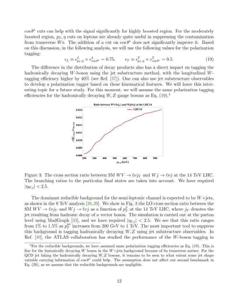
Figure 3: The cross section ratio between SM WV → `νjV and Wj → `νj at the 14 TeV LHC.The branching ratios to the particular final states are taken into account. We have required|ηW,j| < 2.5.
The dominant reducible background for the semi-leptonic channel is expected to be W+jets,as shown in the 8 TeV analysis [38,39]. We show in Fig. 3 the LO cross section ratio between theSM WV → `νjV and Wj → `νj as a function of pVT at the 14 TeV LHC, where jV denotes thejet resulting from hadronic decay of a vector boson. The simulation is carried out at the partonlevel using MadGraph [33], and we have required |ηV,j| < 2.5. We see that this ratio rangesfrom 1% to 1.5% as pjet
T increases from 200 GeV to 1 TeV. The most important tool to suppressthis background is tagging hadronically decaying W,Z using jet substructure observables. InRef. [40], the ATLAS collaboration has studied the performance of the W -boson tagging in
4For the reducible backgrounds, we have assumed same polarization tagging efficiencies as Eq. (19). This isfine for the leptonically decaying W boson in the W+jets background because of its transverse nature. For theQCD jet faking the hadronically decaying W,Z bosons, it remains to be seen to what extent some jet shapevariable carrying information of cos θ∗ could help. The assumption does not affect our second benchmark inEq. (20), as we assume that the reducible backgrounds are negligible.
12

Run 2, and made projections of the efficiency of W -tagging and the rejection of the QCD-jetbackground. A benchmark point in the pjet
T range [500, 1000] GeV for the W -tagging efficiencyis εtag
W = 0.3, while the miss-tagging efficiency for QCD-jet is εmissj = 0.004. Combining this with
the cross section ratio shown in Fig. 3, we could suppress the reducible background W+jetsto the same order of SM WV production in the semi-leptonic channel. Ref. [40] doesn’t showthe results for the W tagging efficiency below 0.3. In an earlier study of Ref. [41], the ATLAScollaboration has shown the W -tagging efficiency below 0.3, but with higher overall mistaggingefficiency for the QCD-jet. For the εtag
W = 0.3, the miss-tagging rate is εmissj = 0.006, while
for εtagW = 0.1, the miss-tagging rate is εmiss
j = 0.0014. Compared with Ref. [41], Ref. [40] has
improved the QCD jet mis-tagging rate by 33% for the εtagW = 0.3. If we assume the same
improvement can be achieved for the case of εtagW = 0.1, the mis-tagging rate for QCD jet
becomes εmissj = 0.0009. The resulting reducible background for WV channel is roughly 20% of
the SM WV process and thus is sub-dominant. In our study, we will assume that for εtagW = 0.1,
the reducible backgrounds can be reduced to a negligible level. We choose the following twobenchmarks for the performance of vector boson tagging.
εtagV = 0.3, nred = nirred
εtagV = 0.1, nred = 0
(20)
where V denotes the hadronically decaying W,Z bosons. nirred is the number of irreduciblebackground events, which comes from SM WV production. nred is the number of reduciblebackground events which mostly comes from SM W+jets production. We have assumed thatthe tagging efficiencies for hadronically decaying Zs and W s are similar.
To summarize, the cross section in the semi-leptonically decaying channel from WV produc-tion is given by
σsemi−lep =∑
p,p′=L,T
σpp′
WW (pT,W > 200 GeV, |ηW | < 2.5)×BRWW→`νjj × εtagV × εp × εp′
+∑
p,p′=L,T
σpp′
WZ(pT,V > 200 GeV, |ηV | < 2.5)×BRWZ→`νjj × εtagV × εp × εp′ ,
(21)
with various efficiencies taking on benchmark values discussed in this section.
3.2 V h production
For the V h(bb) processes, the longitudinal component is dominant in the high-energy regionfor the SM. Therefore, we would not need to worry about contamination from final stateswith transverse polarization. In this case, suppressing the reducible background is essential toenhance the new physics effects. The dominant reducible backgrounds are V bb, tt, and singletop processes. It has been firmly established that the use of jet substructure method can beeffective in separating signal from background in the kinematical regime where Higgs has asizable boost [17, 24]. This is also the regime where new physics effects considered here areenhanced. In particular, Ref. [17] studied the prospect for the discovery of the SM-like Higgs
13

using boosted Higgs tagging method, mainly in the Wh → `νbb channel. They demonstratedthat, in the kinematic region pVT > 200 GeV, a signal to background ratio of SSM/Bred ∼ 0.2is achievable. Here, SSM refers to the rate of SM Wh associated production, while Bred isthe rate of the reducible background. The signal efficiency obtained by the analysis using jetsubstructure in Ref. [17] depending on the pT bins. For the bins [200,400], [400,600], and > 600GeV, the efficiencies are 0.1, 0.2, and 0.3, respectively.5 More recently, Ref. [18] has studied thisSM processes in the 0, 1, and 2-lepton states at the 13 TeV LHC using a combination of boostedHiggs tagging variables. They obtained SSM/Bred ∼ 1 with signal efficiency εtot ∼ 0.1 in thekinematic region pVT > 200 GeV. Of course, such phenomenological studies of the performanceof the Higgs taggers and background rejection power are not fully realistic, they will needto be further studied by the experimental collaborations. At the same time, we also expectpotential improvement both on the optimization of the variables and the reduction experimentalsystematics. In our projection for the potential of HL-LHC, we will use the following benchmark:
εtot = 0.1, nred = nirred (22)
in the 0, 1, and 2 -lepton channels of V h production, focusing on the boosted regions pT,V > 200GeV. Here, nirred refers to the number of events from the SM V h production.
3.3 Reach of the scale of new physics
Based on our analysis of the semi-leptonic channels of di-boson production, we now turn tothe reach of new physics, parameterized by the dimension-6 EFT operators in Eq. (2), throughprecision measurement in this channels. We make projections for the 95% confidence level reachof the scale Λ, denoted as Λ95%, while setting the corresponding Wilson coefficient ci = 1.
As shown in Table 2, production of di-boson final states in the high energy limit only dependson certain combination of the EFT operators. Hence, in generating signal events, it is sufficientto include one of the operators in the combination. In particular, we generate the events usingOHW operator for the combination c
(3)qL , while for the combination cB+cHB−c2B, we use operator
OHB. We are not going to discuss the U(1)Y current-current fermionic operators (OuR,OdR,OqL),
as the sensitivity to them is expected to be similar to that of OHB. We “turn on” one operator ata time. Including multiple operator at the same time can lead to potential correlations and flatdirections. We will leave a more comprehensive treatment for a future study. We first show thebound from WV,Wh channels in each di-boson invariant mass (or equivalently parton center ofmass energy) bin in Fig. 4 for integrated luminosities L = 300fb−1 or L = 3ab−1. For the studiesof semi-leptonically decaying channel of WV by CMS at 8 TeV [38], the systematics is dominatedby the W + jets background normalization, which is around 20%. We expect that significantimprovement in the HL-LHC, and the systematics can be reduced. Similar expectations applyto the V h channels. In making this figure, we have assumed that the systematical error is 5%.For our final combined results presented later, we vary the systematics between 3% and 10%.
For the WV channel, in each di-boson invariant mass bin, we divided the partonic scatteringangle cos θV into four bins [0, 0.2], [0.2, 0.4], [0.4, 0.6], [0.6, 1.0]. Then, we combined the bins
5The number of events in each bin is given by: ni = σ × BR× εitot.
14

ϵL = 0.75, ϵT = 0.5
mWV= Λ95%
L = 3 ab-1, Δsys = 5%
L = 300 fb-1, Δsys = 5%
mWh = Λ95%*4π/g
��� ���� ���� ���� ���� �����
����
����
����
����
��� [���]
��
%[���
]��→��(����) @ ������ ���
(�) = �� ϵ� = ���� ���� = ���
ϵL = 0.75, ϵT = 0.5
mWV= Λ95%
L = 3 ab-1, Δsys = 5%
L = 300 fb-1, Δsys = 5%
mWh = Λ95%*4π/g
��� ���� ���� ���� ���� �����
����
����
����
����
��� [���]
��
%[���
]
��→��(����) @ ������ ���(�) = �� ϵ� = ���� ���� = �
L = 3 ab-1, Δsys = 5%
L = 300 fb-1, Δsys = 5%
mWh= Λ95%
mWh = Λ95%*4π/g
��� ���� ���� ���� �����
����
����
����
����
��� [���]
��
%[���
]
��→��(����) @ ������ ���(�) = �� ϵ = ���� ���� = ���
Figure 4: Λ95%, the 95% lower limit on the scale Λ at the LHC is shown as a function of partoncenter of mass energy mWV . The Wilson coefficient is set to be c
(3)qL = 1, and the limit is set
using channels pp → WV → `νqq (upper two plots) and pp → Wh → `νbb (lower plot) forintegrated luminosities L = 300 fb−1 (solid blue) and L = 3 ab−1 (solid black). The dashedred line, for mWV = Λ95%, is the condition for the consistency of weakly coupled effective fieldtheory. The dashed orange line, for mWV = 4π
gΛ95%, is the condition for the consistency of most
strongly coupled effective field theory (operator enhanced by (4π)2/g2). If the limit Λ95% > mWV
in a particular mWV bin, it is consistent with SM effective field theory. For WV process, wehave explored two benchmark values for the boosted V -jet tagging efficiency and the reduciblebackground, i.e. εV = 0.3, nred = nSM (upper left) and εV = 0.1, nred = 0 (upper right). Inaddition, we assume that the W (V ) polarization tagging efficiencies are εL = 0.75, εT = 0.5.
with number of event greater than 5. This effectively put a cut on cos θV which enhances thelongitudinal new physics signal. From Fig. 4, we can see that higher energy bins, or equivalentlylarger mWV or mWh bins, generically yield better reaches. This is due to the inclusion of thesystematical error, which limits the effectiveness of lower energy bins. For the high-luminosityLHC (L = 3 ab−1), the reach of the cut-off Λ95% in each di-boson invariant mass bin is largerthan the value of mWV (mWh). Therefore, the reach is consistent with effective field assumptions
15
mWV=Λ 95%
L = 3 ab-1, Δsys = 5%
L = 300 fb-1, Δsys = 5%
mWh= Λ95%*
4π /g
��� ���� ���� ���� ���� ���� ���� �����
���
����
����
����
����
����
��� [���]
��
%[���
]��→��(����) @ ������ ��� = �� ϵ� = ���� ���� = ���
mWV=Λ 95%
L = 3 ab-1, Δsys = 5%
L = 300 fb-1, Δsys = 5%
mWh= Λ95%*
4π /g
��� ���� ���� ���� ���� ���� ���� �����
���
����
����
����
����
����
��� [���]
��
%[���
]
��→��(����) @ ������ ��� = �� ϵ� = ���� ���� = �
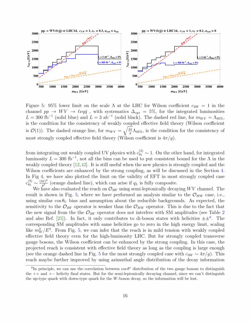
Figure 5: 95% lower limit on the scale Λ at the LHC for Wilson coefficient c3W = 1 in thechannel pp → WV → `νqq , with systematics ∆sys = 5%, for the integrated luminositiesL = 300 fb−1 (solid blue) and L = 3 ab−1 (solid black). The dashed red line, for mWV = Λ95%,is the condition for the consistency of weakly coupled effective field theory (Wilson coefficient
is O(1)). The dashed orange line, for mWV =√
4πg
Λ95%, is the condition for the consistency of
most strongly coupled effective field theory (Wilson coefficient is 4π/g).
from integrating out weakly coupled UV physics with c(3)qL ∼ 1. On the other hand, for integrated
luminosity L = 300 fb−1, not all the bins can be used to put consistent bound for the Λ in theweakly coupled theory [12,42]. It is still useful when the new physics is strongly coupled and theWilson coefficients are enhanced by the strong coupling, as will be discussed in the Section 4.In Fig 4, we have also plotted the limit on the validity of EFT in most strongly coupled case
c(3)qL ∼
(4π)2
g2(orange dashed line), which can arise if qL is fully composite.
We have also evaluated the reach on O3W using semi-leptonically decaying WV channel. Theresult is shown in Fig. 5, where we have performed an analysis similar to the OHW case, i.e.,using similar cos θV bins and assumption about the reducible backgrounds. As expected, thesensitivity to the O3W operator is weaker than the OHW operator. This is due to the fact thatthe new signal from the the O3W operator does not interfere with SM amplitudes (see Table 2and also Ref. [25]). In fact, it only contributes to di-boson states with helicities ±±6. Thecorresponding SM amplitudes with same helicities go to zero in the high energy limit, scalinglike m2
W/E2. From Fig. 5, we can infer that the reach is in mild tension with weakly coupled
effective field theory even for the high-luminosity LHC. But for strongly coupled transversegauge bosons, the Wilson coefficient can be enhanced by the strong coupling. In this case, theprojected reach is consistent with effective field theory as long as the coupling is large enough(see the orange dashed line in Fig. 5 for the most strongly coupled case with c3W ∼ 4π/g). Thisreach maybe further improved by using azimuthal angle distribution of the decay information
6In principle, we can use the correlation between cos θ∗ distribution of the two gauge bosons to distinguishthe ++ and +− helicity final states. But for the semi-leptonically decaying channel, since we can’t distinguishthe up-type quark with down-type quark for the W -boson decay, so the information will be lost.
16

of the W,Z bosons, which results in interference with leading non-vanishing SM amplitude (seeRef. [43, 44]). We will not explore this possibility further here.
cqL(3) = 1, L = 3 ab-1
cqL(3) = 1, L = 300 fb-1
cHB = 1, L = 3 ab-1
cHB = 1, L = 300 fb-1
c3W = 1, L = 3 ab-1
c3W = 1, L = 300 fb-1
�
����
����
����
����
����
��(����) ��(����) ��(����) ��(����)
��%[���
]
����� �� ������ Δ��� ∈ [�%���%]� �� = �
������ ���� ����� ������������OW + OB, LEP S-parameter
OHW - OHB, HL-LHC h → Z γ
OL3 q LEP δgZbL bL
Figure 6: Reach in different channels at the 14 TeV LHC for different combinations of theoperators assuming the systematical error varying from 3% to 10%. The grey and blue regionsdenote the reach of the scale in the case of c
(3)qL = 1 for integrated luminosities L = 3 ab−1
and L = 300 fb−1, respectively. The red and magenta regions denote the reach in the case ofcB + cHB − c2B = 1 for integrated luminosities L = 3 ab−1 and L = 300 fb−1. The orangeand purple regions denote the reach of the size of O3W operator with c3W = 1, for integratedluminosities L = 3 ab−1 and L = 300 fb−1. We also show the present bound from LEP S-parameter on the combination of operators OW and OB with cW + cB = 1 (red dashed line),
the bound from LEP δgZbLbL measurement on the operator c(3)qL = 1/4 (purple dashed line),
based on flavour-universal effects. The case of cHW − cHB = 1 is shown in orange dashed linefrom 3 ab−1 HL-LHC measurement of h → Zγ decay partial width, with a projected precisionof ∼ 20% from Ref. [31].
Finally, we combine all the bins and make projections on the reach of cut-off Λ for differentoperators in different processes. The results are summarized in Fig. 6. We have varied thesystematics from 3% to 10%. For the semi-leptonically decaying WV channel, we only showthe benchmark values for εtag
V = 0.3, nred = nirred. For the second benchmark point of Eq. (20),there is no big difference except the dependence on the systematic uncertainty is weaker. This isbecause of the assumption of zero reducible background. From Fig. 6, we can infer that for thecase of c
(3)qL = 1, the most important bound comes from both Wh(`νbb) and WV (`νjj) channels.
Taking ∆sys = 5% as a benchmark point, the reaches in these two channels are comparable,around 3.8(2.5) TeV in the WV (`νjj) channel for integrated luminosities L = 3 ab−1(300 fb−1),
and 4.0(2.3) TeV for the Wh channel. Note that c(3)qL is the combination of the operators
17

c(3)qL = cW + cHW − c2W + 4c
(3)qL . If we assume that there is no big cancellation in different
Wilson coefficients, we can compare the reach from Di-boson processes with the bound fromEWPT at the LEP and Higgs coupling measurement at the HL-LHC, even though the later twodepend on different combinations of operators (see Table 2 ). The operator OW will contributeto the S-parameter [30, 45]. Suppose it is the dominant contribution, the bound is ∼ 2.5 TeVat 95% CL for cW = 1. OHW will contribute to the Higgs rare process h → Zγ. The h → Zγmeasurement at HL-LHC will put a limit around 1.7 TeV [31] for cHW = 1. For the flavour-
universal operator O(3)qL , from LEP δgZbLbL measurement, the bound is around 1.1 TeV for
c(3)qL = 1/4 [46,47]7. We have shown the three bounds as the red, orange, purple dashed lines in
Fig. 6. The comparison above shows diboson measurement is very promising to probe the newphysics scenario in which the operators considered here give the most important effect. For theoperator O2W , it will contribute to the four fermion operator by equation of motion, especiallyit will contribute to Drell-Yan processes qq → `+`−. This has been studied in Ref. [48] and theexpected reach is 13.4 TeV at the HL-LHC for c2W = 1. Usually, this operator will be suppressedby a factor of g2/g2
∗. However, in certain scenario with strong multi-pole interactions (the socalled Remedios scenario) in Ref. [29], this operator may become as relevant as others. We willdiscuss this in detail in the next section. For the operator combinations of cB + cHB − c2B, thereach is relatively weak (1.3 TeV at the HL-LHC ) from di-boson process. This is a result of thesmallness of the hyper-charge coupling g′. This makes it difficult to compete with S-parameterand hZγ measurement, and the reach is also not consistent with weakly coupled effective fieldtheory. We finally mention that the bound for O3W is 2.4 (1.9)TeV at the 3 ab−1 (300 fb−1),which is also only meaningful if its Wilson coefficient is enhanced by a strong coupling.
4 Reach of new physics scales in different scenarios
In Section 3, we have presented the projection on the reach of Λ in an model independent waywith unit Wilson coefficients (c
(3)qL = 1, c3W = 1 etc). In different new physics scenarios, the
size of Wilson coefficients can be quite different. Assuming that the new physics is broadlycharacterized by a mass scale of new states m∗ and a coupling g∗, the Wilson coefficients are
ci ∼gn∗gnSM
(g2∗
16π2
)nLoop
, n ≤ n(Oi)− 2 (23)
where gSM denotes the SM gauge and Yukawa couplings g, g′, yf . n(Oi) is the number of fields inthe operator Oi. In particular, n(OW,B,HW,HB,3W ) = 3, n(O2W,2B) = 2, and n(OqL,R) = 4. Notethat a covariant derivative is not counted as a field. nLoop is the number of loops needed togenerate the operator. Note that n can also be negative. The bounds Λ95% obtained in theprevious section can be easily translated into the bounds on the mass scale m∗, as functions ofWilson coefficients ci:
m∗ > Λci=195% ×
√ci (24)
7 c(3)qL = 1/4 is chosen such that c
(3)qL = 1 (see Eq. (3)).
18

In the following, we will consider the Strong-Interacting-Light-Higgs (SILH), strong multi-poleinteraction (Remedios), and the (partially) composite fermion scenarios.
4.1 SILH scenario
We start with the SILH scenario [49]. There are two basic assumptions. First, the Higgs and thelongitudinal components of the SM gauge bosons are pseudo-Nambu-Goldstone-bosons associ-ated with the global symmetry breaking in a strongly interacting sector [50]. In addition, the SMfermions acquire masses from their linear mixing with corresponding strongly interacting sectorstates (the so-called partial compositeness [51]). This leads to the following power-countingrules for the Wilson coefficients:
• Each Higgs and Goldstone fields will be associated with a strong coupling g∗ in the op-erators which preserve the global symmetries of the strongly interacting sector, includingthose which are non-linearly realized.
• Explicitly breaking of the strongly interacting sector symmetries will be associated withSM gauge couplings and Yukawa couplings, g, g′, and yf .
Following these rules, we have summarized the size of the Wilson coefficients of the operatorsfor the SILH scenario in the second row of Table 4. None of the operators considered in ourpaper is enhanced by the strong coupling g∗, mainly due to the fact that the transverselypolarized gauge bosons belong to the elementary sector. In the second row of Table 5, wesummarize the reach of the mass scales in the SILH scenario from HL-LHC measurements ofdi-boson, h→ Zγ, h→ γγ [31], and di-lepton processes. For comparison, we have also includedthe bound from S-parameter measurement. In comparison with other measurements, di-bosonprocesses have the best reach in the SILH scenario.
Model O2W O2B O3W OHW OHB OW,B OBBSILH
g2
g2∗
g′2
g2∗
g2
16π2
g2∗16π2
g2∗16π2 1 g2
16π2
Remedios 1 1 g∗g
Remedios+MCHM 1 1 g∗g
1 1 1 1
Remedios+ISO(4) 1 1 g∗g
g∗g
1 1 1
Table 4: Power counting of the size of the Wilson coefficients in different scenario, where g∗ de-notes the coupling in the strong sector. For completeness, we have addedOBB = g′2H†HBµνB
µν .
4.2 Strong multi-pole interaction (Remedios) scenario
Ref. [29] considers the possibility that the SM transverse gauge bosons are part of the strongdynamics. This so called Remedios scenario is based on the observation that the normal SM
19

Model Di-boson S-parameter LHC h→ Zγ LHC h→ γγ LHC dilepton
SILH 4.0 2.5 1.7√
g∗4π
0.34 0.69√
4πg∗
Remedios 10.6√
g∗4π
13.4
Remedios+MCHM 10.6√
g∗4π
2.5 1.7 6.5 13.4
Remedios+ISO(4) 17.6√
g∗4π
2.5 7.5√
g∗4π
6.5 13.4
Table 5: The bounds (in TeV) for different scenarios from different measurements. The LHCmeasurement are prospectives at the integrated luminosity L = 3 ab−1.
gauge interactions (mono-pole) and multi-pole interactions (involving the field strength andits derivatives) have different symmetry structure. Therefore, they can have different couplingstrengths in principle. The small Standard Model couplings, such as g, control the renormalizableinteractions between the gauge boson and the fermions. At the same time, the large coupling g∗determines the strength of the multi-pole interactions of the gauge bosons with the resonancesof the strong sector. This will lead to the following new power-counting rules for the gaugebosons:
• The field strengths of the gauge boson and their derivatives are associated with a strongcoupling g∗, if the interactions preserve the global symmetries of the strong sector. Thenormal gauge interactions are realized by changing the partial derivative to covariantderivative: ∂µ → Dµ = ∂µ − igAµ.
In this case, the O3W operator is enhanced by the strong coupling, while the O2W,2B operatorshave O(1) Wilson coefficients. The power counting of these operators considered in this scenariohave been summarized in the third row of Table 4. We can consider further the scenarios thatboth transverse gauge bosons and Higgs bosons are part of the strong dynamics. Depending onthe symmetry of the strong sector, we have two benchmark scenarios:
• Remedios + MCHM: the symmetry breaking of the strong sector will be SO(5)× SU(2)×U(1)X → SO(4) × SU(2) × U(1)X , where another global symmetry SU(2) is needed tostablize the Higgs potential.
• Remedios +ISO(4): the symmetry breaking of the strong sector will be ISO(4)×U(1)X →SO(4)× U(1)X , where the ISO(4) is the non-compact group SO(4) o T 4.
The corresponding power-counting rules for the size of the Wilson coefficients are presentedin the fourth and fifth rows of Table 4. We summarize the reaches for these three benchmarkscenarios from different measurements of Table 5. Several comments are in order. If only the fieldstrengths are strongly coupled (3rd row), the most relevant operators are O2W with O(1) Wilsoncoefficients and O3W with enhanced Wilson coefficient ∼ O(g∗/g). Di-lepton measurements atHL-LHC will reach 13.4 TeV. The reach from Di-boson measurements are weaker, which is
20

10.6 TeV for the most strongly interacting case g∗ = 4π. The projection is similar for theRemedios + MCHM scenario. For theRemedios + ISO(4) scenario, OHW is enhanced by thestrong coupling g∗. Its Wilson coefficient is g∗/g. As a result, Di-boson measurement can reachhigher ∼ 17.6
√g∗/4π TeV, which becomes better than Di-lepton measurement for large coupling
g∗ & 7.
4.3 Partially Composite fermions
Finally, we discuss the fermionic operators. We focus on the operators O(3)qL , and we expect the
conclusions for other fermionic operators are similar. We will also focus on the flavor-universaleffects, that are invariant under SU(3) flavor transformation. Other effects will be suppressedby the Yukawa couplings under the assumption of minimal flavor violation (MFV) [52]. As
discussed before, the LHC Diboson measurement (Λc(3)qL = 1
4
95% ∼ 4 TeV) will be much better than
the LEP measurement Λc(3)qL = 1
4
95% ∼ 1.1 TeV) for such effects. Now if we assume that the SMfermions have some degrees of compositeness εqL (for example partial compositeness scenario in
Ref. [51]), the size of Wilson coefficient of the O(3)qL by power counting is:
c(3)qLL ∼ 1
4
g2∗g2ε2qL (25)
where we have factored out a 1/4 factor to be consistent with above consideration. The HL-LHCDi-boson measurement will reach the mass scale:
m∗ & 77g∗4πεqL TeV @95%CL (26)
In the meantime, the following four-fermion operator will also be present in the low energyeffective field theory:
L4f =g2∗ε
4qL
m2∗qLγ
µqLqLγµqL (27)
This will lead to energy growing behaviour in the di-jet processes at the LHC. The presentbound from ATLAS di-jet measurement [53] at the 13 TeV with the integrated luminosity of15.7fb−1 is given by (see Ref. [54,55]):
m∗ & 62g∗4π
(εqL)2 TeV @95%CL (28)
Ref. [56] has studied the prospectives on the following operator at the HL-LHC with 13 TeVcenter-of mass energy8:
−g2∗ε
4q
2m2∗
(∑q
qγµTAq
)2
(29)
8Actually, this operator arises from − 12 (DµG
Aµν)2 by equation of motion of the gluon fields.
21

where TA is the generators of QCD SU(3)c group. The expected 95% CL bound on the scale is
m∗ & 83g∗4π
(εqL)2 TeV @95%CL (30)
Although this operator is different from the one in Eq. (27), it can provide a rough idea aboutwhat the scale is probed in the di-jet process at the HL-LHC. We can see that for the smallervalues of εq < 0.9, the LHC Di-boson measurement can be more promising than the di-jetprocess.
5 Conclusions
The future runs of the LHC in the next decade or so will collect nearly thirty times more datathan currently available. There is great potential to improve the precision measurements withthis new data set. The measurements with SM electroweak sector is particularly important, asit is closely related to new physics associated with electroweak symmetry breaking. Studies ofDi-boson channels, V V and V h where V can be SM W and Z, give a promising window intosuch new physics. Such measurements can be complementary to the direct search of new physicsparticles. In certain scenarios, new physics particles can be too heavy to be produced at theLHC. At the same time, their presence can lead to observable effects in precision measurements.
In this paper, we parameterize the new physics effects with dimension 6 EFT operators.We focus on operators which are most relevant for the di-boson final states. In particular, westudy the reach in the semi-leptonic final states. In order to fully take advantage of the largereffect of EFT operators at higher energies, we need to select final states which interfere with theSM background. While this is guaranteed for the V h channel, we have to select longitudinallypolarized W and Z in the WW and WZ channels. There are two possible strategies to achievepolarization tagging. First, the angular distributions of longitudinally and transversely polarizedgauge bosons are different. This effect is most dramatic in the WZ final state with the so calledamplitude zero in the central region for the transverse vector bosons. This has been crucial forthe analysis in the pure leptonic channel [15]. For the semi-leptonic channel we studied here,since we can not distinguish hadronic W and Z very well, this effect is less prominent. Anotherapproach is to directly tag the polarization of the gauge boson by the angular distributionof their decay products. In our study, we use a combination of both approaches. Since theprecision measurements typically focus on cases where S/B is small, the sensitivity dependscrucially on systematic error and background estimates (in particular reducible background).For the reducible background of semi-leptonic WV channel, we have considered the dominantbackground W+jets at parton level and applied the W -tagging efficiency and QCD-jet mis-tagging efficiency based on the study of Ref. [40]. The resulting two benchmarks are summarizedin Eq. (20). For the V h(bb) channel, we have adopted the study of Ref. [18] about the reduciblebackgrounds in the 0,1, and 2 lepton channels, which leads to Eq. (22) as our benchmark in thesechannels. Our results shows that precision measurement at the LHC can have good sensitivityin probing new physics at multiple-TeV scale. It can surpass the sensitivity of LEP precisionmeasurements, such as those from the S-parameter and Z coupling measurements. Compared
22

with fully leptonic decaying WZ channels, the semi-leptonic decay WV channel has order ofmagnitude larger rate. At the same time, semi-leptonic decay channels suffer from large reduciblebackgrounds. During the up coming runs of the LHC, we expect significant improvement inunderstanding the reducible background and reducing systematics. Anticipating this, we makeoptimistic projections of the reducible background for the semi-leptonic decay channels based
on extrapolations of ATLAS study. Based on this, our result (Λc(3)qL
95% ∼ 4 TeV) is better than
the fully leptonic WZ channel (Λc(3)qL
95% ∼ 3.2 TeV) studied in Ref. [15]. As an application of ourresult, we derived the reach of the new physics scale in several new physics scenarios. In the SILHscenario, which models the generic feature of composite Higgs models, the diboson measurementcan be more sensitive than other experimental observables. For the scenario with strong multipleinteractions (the so called Remedios), di-boson is either slightly weaker or comparable with themeasurements in di-lepton channel.
It is worth emphasizing that the estimates we made here are based on our assumptionsabout systematics and efficiencies achievable at the HL-LHC. More detailed and realistic studies,presumably based on real data and full fledged simulations, would be necessary to determine theprecise reach. In this sense, the numbers presented here are better considered as benchmarksor targets, which could give us good reach in these channels. We have also identified severaldirections in which improvements can be crucial to enhance the sensitivity in the di-bosonchannel. Obviously, any new technique to tag the polarization of the vector bosons can be veryhelpful. A major direction to pursue is the tagging of polarization of the hadronic W and Z. Inaddition, distinguishing hadronic W and Z can also be very helpful in enhancing longitudinalfinal states.
6 Acknowledgement
We are grateful to Andrea Tesi for numerous helpful discussion and collaboration during theearly stages of this work. We would also like to thank Francesco Riva, Andrea Wulzer forhelpful discussions and thank Nurfikri Norjoharuddeen, Oliver Majersky and Ece Akilli forbringing Ref. [41] to our attention. LTW is supported by the DOE grant DE-SC0013642. DL issupported in part by the U.S. Department of Energy under Contract No. DE-AC02-06CH11357.
A Cross sections of the Di-boson processes at the LHC
In Table 6, we have reported the cross section for the di-boson processes at the 14TeV LHCas a function of the cut-off Λ in each pT bin with the Wilson coefficient cHW setting to one.The cross sections are calculated using MadGraph [33] at LO simulation with parton level cuts|ηW,Z,h| < 2.5. We can see clearly that the new physics effects manifest in the purely longitudinalhelicity final states of W,Z gauge bosons and the Higgs boson with energy growing behaviour.It results in the fact that the coefficients of 1/Λ2 become larger as the pT increases. In addition,the ratios between the coefficients of 1/Λ4 and that of 1/Λ2 grow as the pT becomes larger,
23

which indicates that the larger value of Λ is needed for 1/Λ2 terms dominate. For the processesincluding one transverse gauge bosons and one longitudinal gauge bosons (including the Higgsboson), the cross sections are comparable to the transverse one in the low pT bin [0, 400] GeV anddecrease very fast as pT increases. It results in below 5% of LL one for the WW,WZ processesand below 1% of VLh for the V h processes for the largest pT bin. For the SM WW , the purelytransverse helicity final states TT dominate over LL by a factor of 16 in the moderately boostedregion pT ∈ [200, 400] GeV and a factor of 12 in the highly boosted region pT ∈ [1000, 1500]GeV. While for the WZ process, the TT cross section is only a factor of 3 of the LL one in themoderately boosted region and becomes comparable to LL in the highly boosted bin. This isdue to amplitude zero in this process as discussed in the main text.
σ [fb], pT [GeV] [0,200] [200, 400] [400,600]
W±L ZL 784(1 + 0.116
Λ2 + 0.00625Λ4
)58.5
(1 + 0.682
Λ2 + 0.141Λ4
)4.84
(1 + 2.09
Λ2 + 1.24Λ4
)W±L(T )ZT (L) 1614
(1 + 0.0610
Λ2 + 0.00181Λ4
)23.0
(1 + 0.419
Λ2 + 0.0611Λ4
)0.598
(1 + 1.40
Λ2 + 0.623Λ4
)W±T ZT 5755 164 12.0
W+LW
−L 1416
(1 + 0.0318
Λ2 + 0.00203Λ4
)34.0
(1 + 0.597
Λ2 + 0.121Λ4
)2.75
(1 + 1.83
Λ2 + 1.05Λ4
)W+L(T )W
−T (L) 4866
(1 + 0.00758
Λ2 + 0.000489Λ4
)34.6
(1 + 0.130
Λ2 + 0.0207Λ4
)0.848
(1 + 0.429
Λ2 + 0.213Λ4
)W+T W
−T 17987 523 39.1
W±L h 387(1 + 0.149
Λ2 + 0.00776Λ4
)46.5
(1 + 0.712
Λ2 + 0.148Λ4
)4.30
(1 + 2.13
Λ2 + 1.24Λ4
)W±T h 270
(1 + 0.0302
Λ2 + 0.000146Λ4
)4.93
(1 + 0.0287
Λ2 + 0.000217Λ4
)0.140
(1 + 0.0271
Λ2 + 0.000275Λ4
)ZLh 198
(1 + 0.134
Λ2 + 0.00731Λ4
)24.5
(1 + 0.628
Λ2 + 0.136Λ4
)2.24
(1 + 1.90
Λ2 + 1.14Λ4
)ZTh 154
(1 + 0.0361
Λ2 + 0.000353Λ4
)3.30
(1 + 0.0688
Λ2 + 0.00501Λ4
)0.0941
(1 + 0.165
Λ2 + 0.0413Λ4
)σ [fb], pT [GeV] [600,800] [800,1000] [1000,1500]
W±L ZL 0.799(1 + 4.30
Λ2 + 4.87Λ4
)0.188
(1 + 6.92
Λ2 + 13.4Λ4
)0.0749
(1 + 11.9
Λ2 + 39.1Λ4
)W±L(T )ZT (L) 0.0471
(1 + 2.91
Λ2 + 2.60Λ4
)0.00634
(1 + 4.89
Λ2 + 7.34Λ4
)0.00149
(1 + 8.01
Λ2 + 20.6Λ4
)W±T ZT 1.74 0.357 0.121
W+LW
−L 0.442
(1 + 3.74
Λ2 + 4.13Λ4
)0.102
(1 + 6.13
Λ2 + 11.4Λ4
)0.0405
(1 + 10.4
Λ2 + 32.6Λ4
)W+L(T )W
−T (L) 0.0652
(1 + 0.888
Λ2 + 0.889Λ4
)0.00873
(1 + 1.49
Λ2 + 2.47Λ4
)0.00204
(1 + 2.43
Λ2 + 6.79Λ4
)W+T W
−T 5.92 1.28 0.475
W±L h 0.726(1 + 4.22
Λ2 + 4.83Λ4
)0.169
(1 + 7.15
Λ2 + 13.3Λ4
)0.0671
(1 + 12.2
Λ2 + 38.7Λ4
)W±T h 0.0112
(1 + 0.0283
Λ2 + 0.000218Λ4
)0.00153 0.000364
ZLh 0.367(1 + 3.82
Λ2 + 4.50Λ4
)0.0835
(1 + 6.27
Λ2 + 12.4Λ4
)0.0327
(1 + 11.0
Λ2 + 35.9Λ4
)ZTh 0.00737
(1 + 0.318
Λ2 + 0.165Λ4
)0.000991
(1 + 0.523
Λ2 + 0.455Λ4
)0.000231
(1 + 0.838
Λ2 + 1.24Λ4
)
Table 6: Helicity cross sections (in fb) for the di-boson processes at the 14 TeV LHC as afunction of the cut-off Λ (in TeV) in each pT bin with the Wilson coefficient cHW setting to one.
24

B Polarization measurement of the W boson
To measure the W polarization, we need to study the angular distribution of its decay products.We choose the polarization axis to be the direction of the W in the laboratory frame. Theamplitude for the W+(pW )→ l+(p`)ν(pν) is:
M =g√2uL(pν)γ
µνL(p`)ε∗µ(pW ) (31)
Let’s start from the rest frame of the W+. We parametrize the momenta of leptons as follows:
p∗` = (k,~k) = (k, k sin θ∗ cosϕ∗, k sin θ∗ sinϕ∗, k cos θ∗),
p∗ν = (k,−~k) = (k,−k sin θ∗ cosϕ∗,−k sin θ∗ sinϕ∗,−k cos θ∗)(32)
where k = |~k| = mW/2. The general expressions for the helicity spinors are given by:
ξL(p∗`) =
(−e−iϕ∗/2 sin θ∗
2
eiϕ∗/2 cos θ∗
2
), ξR(p∗`) =
(e−iϕ
∗/2 cos θ∗
2
eiϕ∗/2 sin θ∗
2
)ξL(p∗ν) =
(e−iϕ
∗/2 cos θ∗
2
eiϕ∗/2 sin θ∗
2
), ξR(p∗ν) =
(−e−iϕ∗/2 sin θ∗
2
eiϕ∗/2 cos θ∗
2
) (33)
and the left-handed current is as follows:
uL(p∗ν)γµνL(p∗`) = 2k(0,−eiϕ∗ cos2 θ
∗
2+ e−iϕ
∗sin2 θ
∗
2, ieiϕ
∗cos2 θ
∗
2+ ie−iϕ
∗sin2 θ
∗
2, sin θ∗)µ (34)
By using the formulae of the polarization vectors:
ε+µ =1√2
01i0
, ε−µ =1√2
01−i0
, ε0µ =
0001
, (35)
we can easily obtain the helicity amplitudes:
M+ = −gke−iϕ∗(1− cos θ∗), M− = gkeiϕ8
(1 + cos θ∗), M0 = −√
2gk sin θ∗ (36)
which leads to the distribution in Eq. (15). Turn to the laboratory frame and suppose that wecan reconstruct the z-momentum of the neutrino by imposing the condition that the system oflepton-neutrino should correctly reproduce the mass of the W boson. The momentum of thecharged lepton and neutrino in the laboratory frame can be obtained from the momentum inthe W+ rest frame by a Lorentz boost:
E` = γ(k + ~v · ~k
), ~p` = ~k + ~v
(γk +
γ − 1
v2~v · ~k
)Eν = γ
(k − ~v · ~k
), ~pν = −~k + ~v
(γk − γ − 1
v2~v · ~k
) (37)
25

where ~v = ~pWEW
, v = |~v| is the velocity of the W+ in the laboratory frame. Then the formulaeof cos θ∗ can be obtained by the energy difference of the lepton and neutrino in the laboratoryframe as follows:
cos θ∗ =~v · ~kkv
=E` − Eν|~pW |
=|~p`| − |~pν ||~p` + ~pν |
(38)
where we have used:k =
mW
2, |~pW | = mWγv (39)
References
[1] B. Grzadkowski, M. Iskrzynski, M. Misiak, and J. Rosiek, Dimension-Six Terms in the StandardModel Lagrangian, JHEP 10 (2010) 085, [arXiv:1008.4884].
[2] J. Elias-Miro, J. R. Espinosa, E. Masso, and A. Pomarol, Higgs windows to new physics throughd=6 operators: constraints and one-loop anomalous dimensions, JHEP 11 (2013) 066,[arXiv:1308.1879].
[3] R. Contino, M. Ghezzi, C. Grojean, M. Muhlleitner, and M. Spira, Effective Lagrangian for alight Higgs-like scalar, JHEP 07 (2013) 035, [arXiv:1303.3876].
[4] Tevatron Electroweak Working Group, CDF, DELPHI, SLD Electroweak and HeavyFlavour Groups, ALEPH, LEP Electroweak Working Group, SLD, OPAL, D0, L3Collaboration, L. E. W. Group, Precision Electroweak Measurements and Constraints on theStandard Model, arXiv:1012.2367.
[5] J. Ellis, V. Sanz, and T. You, Complete Higgs Sector Constraints on Dimension-6 Operators,JHEP 07 (2014) 036, [arXiv:1404.3667].
[6] A. Falkowski and F. Riva, Model-independent precision constraints on dimension-6 operators,JHEP 02 (2015) 039, [arXiv:1411.0669].
[7] A. Falkowski, M. Gonzalez-Alonso, A. Greljo, and D. Marzocca, Global constraints on anomaloustriple gauge couplings in effective field theory approach, Phys. Rev. Lett. 116 (2016), no. 1011801, [arXiv:1508.00581].
[8] A. Butter, O. J. P. Eboli, J. Gonzalez-Fraile, M. C. Gonzalez-Garcia, T. Plehn, and M. Rauch,The Gauge-Higgs Legacy of the LHC Run I, JHEP 07 (2016) 152, [arXiv:1604.03105].
[9] Z. Zhang, Time to Go Beyond Triple-Gauge-Boson-Coupling Interpretation of W PairProduction, Phys. Rev. Lett. 118 (2017), no. 1 011803, [arXiv:1610.01618].
[10] A. Falkowski, M. Gonzalez-Alonso, A. Greljo, D. Marzocca, and M. Son, Anomalous TripleGauge Couplings in the Effective Field Theory Approach at the LHC, JHEP 02 (2017) 115,[arXiv:1609.06312].
[11] D. R. Green, P. Meade, and M.-A. Pleier, Multiboson interactions at the LHC, Rev. Mod. Phys.89 (2017), no. 3 035008, [arXiv:1610.07572].
26

[12] A. Biekotter, A. Knochel, M. Kramer, D. Liu, and F. Riva, Vices and virtues of Higgs effectivefield theories at large energy, Phys. Rev. D91 (2015) 055029, [arXiv:1406.7320].
[13] J. Baglio, S. Dawson, and I. M. Lewis, An NLO QCD effective field theory analysis of W+W−
production at the LHC including fermionic operators, Phys. Rev. D96 (2017), no. 7 073003,[arXiv:1708.03332].
[14] J. Ellis, C. W. Murphy, V. Sanz, and T. You, Updated Global SMEFT Fit to Higgs, Diboson andElectroweak Data, arXiv:1803.03252.
[15] R. Franceschini, G. Panico, A. Pomarol, F. Riva, and A. Wulzer, Electroweak Precision Tests inHigh-Energy Diboson Processes, JHEP 02 (2018) 111, [arXiv:1712.01310].
[16] M. Chiesa, A. Denner, and J.-N. Lang, Anomalous triple-gauge-boson interactions invector-boson pair production with RECOLA2, arXiv:1804.01477.
[17] J. M. Butterworth, I. Ochoa, and T. Scanlon, Boosted Higgs → bb in vector-boson associatedproduction at 14 TeV, Eur. Phys. J. C75 (2015), no. 8 366, [arXiv:1506.04973].
[18] F. Tian, Combined analysis of jet substructure for Higgs decay to bb in vector boson associatedproduction at the 13 TeV LHC, arXiv:1701.08413.
[19] M. S. Chanowitz and M. K. Gaillard, The TeV Physics of Strongly Interacting W’s and Z’s,Nucl. Phys. B261 (1985) 379–431.
[20] A. Wulzer, An Equivalent Gauge and the Equivalence Theorem, Nucl. Phys. B885 (2014)97–126, [arXiv:1309.6055].
[21] R. Contino, C. Grojean, M. Moretti, F. Piccinini, and R. Rattazzi, Strong Double HiggsProduction at the LHC, JHEP 05 (2010) 089, [arXiv:1002.1011].
[22] M. Szleper, The Higgs boson and the physics of WW scattering before and after Higgs discovery,arXiv:1412.8367.
[23] K. Hagiwara, R. D. Peccei, D. Zeppenfeld, and K. Hikasa, Probing the Weak Boson Sector ine+e− →W+W−, Nucl. Phys. B282 (1987) 253–307.
[24] J. M. Butterworth, A. R. Davison, M. Rubin, and G. P. Salam, Jet substructure as a new Higgssearch channel at the LHC, Phys. Rev. Lett. 100 (2008) 242001, [arXiv:0802.2470].
[25] A. Azatov, R. Contino, C. S. Machado, and F. Riva, Helicity selection rules and noninterferencefor BSM amplitudes, Phys. Rev. D95 (2017), no. 6 065014, [arXiv:1607.05236].
[26] U. Baur, T. Han, and J. Ohnemus, Amplitude zeros in W±Z production, Phys. Rev. Lett. 72(1994) 3941–3944, [hep-ph/9403248].
[27] C. Frye, M. Freytsis, J. Scholtz, and M. J. Strassler, Precision Diboson Observables for the LHC,JHEP 03 (2016) 171, [arXiv:1510.08451].
[28] T. Han, D. Krohn, L.-T. Wang, and W. Zhu, New Physics Signals in Longitudinal Gauge BosonScattering at the LHC, JHEP 03 (2010) 082, [arXiv:0911.3656].
27

[29] D. Liu, A. Pomarol, R. Rattazzi, and F. Riva, Patterns of Strong Coupling for LHC Searches,JHEP 11 (2016) 141, [arXiv:1603.03064].
[30] M. E. Peskin and T. Takeuchi, Estimation of oblique electroweak corrections, Phys. Rev. D46(1992) 381–409.
[31] S. Dawson et al., Working Group Report: Higgs Boson, in Proceedings, 2013 CommunitySummer Study on the Future of U.S. Particle Physics: Snowmass on the Mississippi (CSS2013):Minneapolis, MN, USA, July 29-August 6, 2013, 2013. arXiv:1310.8361.
[32] A. Alloul, N. D. Christensen, C. Degrande, C. Duhr, and B. Fuks, FeynRules 2.0 - A completetoolbox for tree-level phenomenology, Comput. Phys. Commun. 185 (2014) 2250–2300,[arXiv:1310.1921].
[33] J. Alwall, R. Frederix, S. Frixione, V. Hirschi, F. Maltoni, O. Mattelaer, H. S. Shao, T. Stelzer,P. Torrielli, and M. Zaro, The automated computation of tree-level and next-to-leading orderdifferential cross sections, and their matching to parton shower simulations, JHEP 07 (2014)079, [arXiv:1405.0301].
[34] R. D. Ball et al., Parton distributions with LHC data, Nucl. Phys. B867 (2013) 244–289,[arXiv:1207.1303].
[35] CMS Collaboration, S. Goy Lopez, CMS Detector Performance during LHC Run 1 andprojections for Run 2, Nucl. Part. Phys. Proc. 273-275 (2016) 1048–1054.
[36] ATLAS Collaboration, G. Aad et al., Expected Performance of the ATLAS Experiment -Detector, Trigger and Physics, arXiv:0901.0512.
[37] CMS Collaboration, V. Khachatryan et al., Identification techniques for highly boosted W bosonsthat decay into hadrons, JHEP 12 (2014) 017, [arXiv:1410.4227].
[38] CMS Collaboration, A. M. Sirunyan et al., Search for anomalous couplings in boostedWW/WZ→ `νqq production in proton-proton collisions at
√s = 8 TeV, Phys. Lett. B772
(2017) 21–42, [arXiv:1703.06095].
[39] ATLAS Collaboration, M. Aaboud et al., Measurement of WW/WZ → `νqq′ production withthe hadronically decaying boson reconstructed as one or two jets in pp collisions at
√s = 8 TeV
with ATLAS, and constraints on anomalous gauge couplings, Eur. Phys. J. C77 (2017), no. 8563, [arXiv:1706.01702].
[40] ATLAS Collaboration, T. A. collaboration, Performance of Top Quark and W Boson Taggingin Run 2 with ATLAS, .
[41] Identification of boosted, hadronically-decaying W and Z bosons in√s = 13 TeV Monte Carlo
Simulations for ATLAS, Tech. Rep. ATL-PHYS-PUB-2015-033, CERN, Geneva, Aug, 2015.
[42] R. Contino, A. Falkowski, F. Goertz, C. Grojean, and F. Riva, On the Validity of the EffectiveField Theory Approach to SM Precision Tests, JHEP 07 (2016) 144, [arXiv:1604.06444].
28

[43] A. Azatov, J. Elias-Miro, Y. Reyimuaji, and E. Venturini, Novel measurements of anomaloustriple gauge couplings for the LHC, JHEP 10 (2017) 027, [arXiv:1707.08060].
[44] G. Panico, F. Riva, and A. Wulzer, Diboson Interference Resurrection, Phys. Lett. B776 (2018)473–480, [arXiv:1708.07823].
[45] R. Barbieri, A. Pomarol, R. Rattazzi, and A. Strumia, Electroweak symmetry breaking afterLEP-1 and LEP-2, Nucl. Phys. B703 (2004) 127–146, [hep-ph/0405040].
[46] A. Pomarol and F. Riva, Towards the Ultimate SM Fit to Close in on Higgs Physics, JHEP 01(2014) 151, [arXiv:1308.2803].
[47] J. Ellis, V. Sanz, and T. You, The Effective Standard Model after LHC Run I, JHEP 03 (2015)157, [arXiv:1410.7703].
[48] M. Farina, G. Panico, D. Pappadopulo, J. T. Ruderman, R. Torre, and A. Wulzer, Energy helpsaccuracy: electroweak precision tests at hadron colliders, Phys. Lett. B772 (2017) 210–215,[arXiv:1609.08157].
[49] G. F. Giudice, C. Grojean, A. Pomarol, and R. Rattazzi, The Strongly-Interacting Light Higgs,JHEP 06 (2007) 045, [hep-ph/0703164].
[50] K. Agashe, R. Contino, and A. Pomarol, The Minimal composite Higgs model, Nucl. Phys. B719(2005) 165–187, [hep-ph/0412089].
[51] D. B. Kaplan, Flavor at SSC energies: A New mechanism for dynamically generated fermionmasses, Nucl. Phys. B365 (1991) 259–278.
[52] G. D’Ambrosio, G. F. Giudice, G. Isidori, and A. Strumia, Minimal flavor violation: AnEffective field theory approach, Nucl. Phys. B645 (2002) 155–187, [hep-ph/0207036].
[53] ATLAS Collaboration, T. A. collaboration, Search for New Phenomena in Dijet Events with theATLAS Detector at
√s=13 TeV with 2015 and 2016 data, .
[54] B. Bellazzini, F. Riva, J. Serra, and F. Sgarlata, The other effective fermion compositeness,JHEP 11 (2017) 020, [arXiv:1706.03070].
[55] O. Domenech, A. Pomarol, and J. Serra, Probing the SM with Dijets at the LHC, Phys. Rev.D85 (2012) 074030, [arXiv:1201.6510].
[56] S. Alioli, M. Farina, D. Pappadopulo, and J. T. Ruderman, Precision Probes of QCD at HighEnergies, JHEP 07 (2017) 097, [arXiv:1706.03068].
29