Preconditioners for Karush–Kuhn–Tucker Systemsarising in Optimal Control

Astrid Battermann

Thesis submitted to the Faculty of the Virginia Polytechnic Institute and State Universityin partial fulfillment of the requirements for the degree of

MASTER OF SCIENCEIN

MATHEMATICS

APPROVED:Matthias Heinkenschloss, Chair

Christopher BeattieJohn A. Burns

June 14, 1996Blacksburg, Virginia

Keywords: Preconditioning, Karush–Kuhn–Tucker Systems, Indefinite Systems,Quadratic Programming, Optimal Control

Copyright 1996, Astrid Battermann

PRECONDITIONERS FOR KARUSH–KUHN–TUCKER SYSTEMSARISING IN OPTIMAL CONTROL

Astrid Battermann

Committee Chairman: Dr. Matthias Heinkenschloss

Mathematics

(ABSTRACT)

This work is concerned with the construction of preconditioners for indefinite linear sys-tems. The systems under investigation arise in the numerical solution of quadratic pro-gramming problems, for example in the form of Karush–Kuhn–Tucker (KKT) optimalityconditions or in interior–point methods. Therefore, the system matrix is referred to as aKKT matrix. It is not the purpose of this thesis to investigate systems arising from generalquadratic programming problems, but to study systems arising in linear quadratic controlproblems governed by partial differential equations.

The KKT matrix is symmetric, nonsingular, and indefinite. For the solution of the lin-ear systems generalizations of the conjugate gradient method, MINRES and SYMMLQ, areused. The performance of these iterative solution methods depends on the eigenvalue distri-bution of the matrix and of the cost of the multiplication of the system matrix with a vector.To increase the performance of these methods, one tries to transform the system to favorablychange its eigenvalue distribution. This is called preconditioning and the nonsingular trans-formation matrices are called preconditioners. Since the overall performance of the iterativemethods also depends on the cost of matrix–vector multiplications, the preconditioner hasto be constructed so that it can be applied efficiently.

The preconditioners designed in this thesis are positive definite and they maintain thesymmetry of the system. For the construction of the preconditioners we strongly exploit thestructure of the underlying system. The preconditioners are composed of preconditionersfor the submatrices in the KKT system. Therefore, known efficient preconditioners can bereadily adapted to this context. The derivation of the preconditioners is motivated by theproperties of the KKT matrices arising in optimal control problems. An analysis of thepreconditioners is given and various cases which are important for interior point methodsare treated separately. The preconditioners are tested on a typical problem, a Neumannboundary control for an elliptic equation. In many important situations the preconditionerssubstantially reduce the number of iterations needed by the solvers. In some cases, it caneven be shown that the number of iterations for the preconditioned system is independentof the refinement of the discretization of the partial differential equation.

Acknowledgments

I would like to express my sincere gratitude to my advisor and committee chairman, Dr.Matthias Heinkenschloss, for his support and guidance which made this work possible.

I want to thank Dr. Burns and Dr. Beattie for serving on my committee. They werealways encouraging and supportive.

Special thanks to all people in ICAM. I am glad that I got to know them.

I owe a lot to my parents. Their support was very important during this year.

iii

Contents

1 Introduction 11.1 Motivation . . . . . . . . . . . . . . . . . . . . . . . . . . . . . . . . . . . . . 11.2 Outline of the Thesis . . . . . . . . . . . . . . . . . . . . . . . . . . . . . . . 3

2 The Quadratic Programming Problem and the KKT Matrix 42.1 The Quadratic Programming Problem . . . . . . . . . . . . . . . . . . . . . 42.2 Interior–Point Methods for the Solution of the Quadratic Programming Problem 62.3 Three Cases . . . . . . . . . . . . . . . . . . . . . . . . . . . . . . . . . . . . 8

2.3.1 No Bound Constraints . . . . . . . . . . . . . . . . . . . . . . . . . . 82.3.2 Bound Constraints for u . . . . . . . . . . . . . . . . . . . . . . . . . 82.3.3 Bound Constraints for u and y . . . . . . . . . . . . . . . . . . . . . . 9

3 Eigenvalue Estimates 123.1 The Eigenvalue Distribution . . . . . . . . . . . . . . . . . . . . . . . . . . . 123.2 A Theorem by Rusten and Winther . . . . . . . . . . . . . . . . . . . . . . . 13

4 SYMMLQ AND MINRES 164.1 Introduction to SYMMLQ and MINRES . . . . . . . . . . . . . . . . . . . . 164.2 Derivation of SYMMLQ and MINRES . . . . . . . . . . . . . . . . . . . . . 174.3 Convergence Analysis . . . . . . . . . . . . . . . . . . . . . . . . . . . . . . . 20

4.3.1 Convergence Results for MINRES . . . . . . . . . . . . . . . . . . . . 244.3.2 Convergence Results for SYMMLQ . . . . . . . . . . . . . . . . . . . 34

4.4 Implementation of SYMMLQ and MINRES . . . . . . . . . . . . . . . . . . 344.4.1 Orthogonal Bases for the Krylov Subspaces . . . . . . . . . . . . . . . 374.4.2 SYMMLQ . . . . . . . . . . . . . . . . . . . . . . . . . . . . . . . . . 414.4.3 MINRES . . . . . . . . . . . . . . . . . . . . . . . . . . . . . . . . . . 48

5 Preconditioning 525.1 The Issue of Preconditioning . . . . . . . . . . . . . . . . . . . . . . . . . . . 525.2 The Preconditioned Algorithms . . . . . . . . . . . . . . . . . . . . . . . . . 53

iv

6 The Preconditioners 616.1 Introduction . . . . . . . . . . . . . . . . . . . . . . . . . . . . . . . . . . . . 616.2 The First Preconditioner . . . . . . . . . . . . . . . . . . . . . . . . . . . . . 63

6.2.1 Derivation of the First Preconditioner . . . . . . . . . . . . . . . . . . 636.2.2 Expected Performance of the First Preconditioner . . . . . . . . . . . 676.2.3 Comparison with Gill, Murray, Ponceleon and Saunders . . . . . . . . 696.2.4 Application of the First Preconditioner . . . . . . . . . . . . . . . . . 70

6.3 The Second Preconditioner . . . . . . . . . . . . . . . . . . . . . . . . . . . . 706.3.1 Derivation of the Ideal Second Preconditioner . . . . . . . . . . . . . 716.3.2 Derivation of the General Second Preconditioner . . . . . . . . . . . . 726.3.3 Expected Performance of the Second Preconditioner . . . . . . . . . . 746.3.4 Application of the Second Preconditioner . . . . . . . . . . . . . . . . 756.3.5 Quality of the Solution . . . . . . . . . . . . . . . . . . . . . . . . . . 76

6.4 The Third Preconditioner . . . . . . . . . . . . . . . . . . . . . . . . . . . . 796.4.1 Derivation of the Third Preconditioner . . . . . . . . . . . . . . . . . 796.4.2 Expected Performance of the Third Preconditioner . . . . . . . . . . 806.4.3 Application of the Third Preconditioner . . . . . . . . . . . . . . . . 816.4.4 Quality of the Solution . . . . . . . . . . . . . . . . . . . . . . . . . . 82

7 Applications 857.1 Neumann Control for an Elliptic Equation . . . . . . . . . . . . . . . . . . . 857.2 The Problem Discretization . . . . . . . . . . . . . . . . . . . . . . . . . . . 857.3 Eigenvalues of FEM Matrices . . . . . . . . . . . . . . . . . . . . . . . . . . 887.4 Condition Number of the KKT–System . . . . . . . . . . . . . . . . . . . . . 907.5 Numerical Results without a Preconditioner . . . . . . . . . . . . . . . . . . 927.6 Numerical Results with the First Preconditioner . . . . . . . . . . . . . . . . 1007.7 Numerical Results with the Second Preconditioner . . . . . . . . . . . . . . . 1097.8 Numerical Results with the Third Preconditioner . . . . . . . . . . . . . . . 117

8 Conclusion and Future Work 1258.1 Conclusion . . . . . . . . . . . . . . . . . . . . . . . . . . . . . . . . . . . . . 1258.2 Future Work . . . . . . . . . . . . . . . . . . . . . . . . . . . . . . . . . . . . 126

v

List of Figures

7.1 The grid for nx = ny = 5. . . . . . . . . . . . . . . . . . . . . . . . . . . . . 867.2 The eigenvalues and singular values of the submatrices in K for nx = ny = 20

and α = 1, Dy = 0, Du = 0. . . . . . . . . . . . . . . . . . . . . . . . . . . . 947.3 The eigenvalues of the KKT–system for nx = ny = 20 and α = 1, Dy = 0,

Du = 0. . . . . . . . . . . . . . . . . . . . . . . . . . . . . . . . . . . . . . . 957.5 The eigenvalues and singular values of the submatrices before preconditioning

for a grid nx = ny = 20 with Du = 104 · I , Du = 0, α = 1. . . . . . . . . . . 977.6 The eigenvalues of the KKT-system before preconditioning for nx = ny = 20

with Du = 104 · I , Dy = 0, α = 1. . . . . . . . . . . . . . . . . . . . . . . . . 977.7 The eigenvalues of the KKT–system before preconditioning for nx = ny = 20

with Dy = 104 · I , Du = 0, α = 1 . . . . . . . . . . . . . . . . . . . . . . . . 987.4 The residuals, the absolute and the relative error of MINRES– and SYMMLQ–

iterates on the system K for nx = ny = 5 with Dy = 0, Du = 0, α = 1. . . . 997.8 The eigenvalues and singular values of the preconditioned submatrices in

P−11 KP−T1 with α = 1, Dy = 0, Du = 0 for nx = ny = 20. . . . . . . . . . . . 102

7.9 The eigenvalues of the preconditioned KKT–matrix P−11 KP−T1 with α = 1,

Dy = 0, Du = 0 for nx = ny = 20. . . . . . . . . . . . . . . . . . . . . . . . . 1037.10 The eigenvalues and singular values of the submatrices in P−1

1 KP−T1 withDu = 104 · I , Dy = 0, α = 1 for nx = ny = 20. . . . . . . . . . . . . . . . . . 105

7.11 The eigenvalues of P−11 KP−T1 with Du = 104 · I , Dy = 0, α = 1 for nx = ny =

20. . . . . . . . . . . . . . . . . . . . . . . . . . . . . . . . . . . . . . . . . 1057.13 The eigenvalues of P−1

1 KP−T1 with Dy = 104 · I , Du = 0, α = 1 for nx = ny =20. . . . . . . . . . . . . . . . . . . . . . . . . . . . . . . . . . . . . . . . . 107

7.12 The residuals, the absolute and the relative error of MINRES– and SYMMLQ–iterates on the system P−1

1 KP−T1 for nx = ny = 5 with α = 1, Dy = 0, Du = 0. 1087.14 The eigenvalues and singular values of the preconditioned submatrices in

P−12 KP−T2 for nx = ny = 20, α = 1, Dy = 0, Du = 0. . . . . . . . . . . . . . 110

7.15 The eigenvalues of the preconditioned KKT–matrix P−12 KP−T2 for nx = ny =

20, α = 1, Dy = 0, Du = 0. . . . . . . . . . . . . . . . . . . . . . . . . . . . 1117.16 The eigenvalues of the KKT matrix P−1

2 KP−T2 with Dy = 104 · I , α = 1,Du = 0 for nx = ny = 20. . . . . . . . . . . . . . . . . . . . . . . . . . . . . 114

vi

7.17 The residuals, the absolute and the relative error of MINRES– and SYMMLQ–iterates on the system P−1

2 KP−T2 for nx = ny = 10 with Dy = 0, Du = 0,α = 1. . . . . . . . . . . . . . . . . . . . . . . . . . . . . . . . . . . . . . . . 115

7.18 The residuals, the absolute and the relative error of MINRES– and SYMMLQ–iterates on the system P−1

2 KP−T2 for nx = ny = 10 with Dy = 0, Du = 0,α = 10−5. . . . . . . . . . . . . . . . . . . . . . . . . . . . . . . . . . . . . . 116

7.19 The eigenvalues of the submatrices in P−13 KP−T3 for nx = ny = 20, α = 1,

Dy = 0, Du = 0. . . . . . . . . . . . . . . . . . . . . . . . . . . . . . . . . . 1187.20 The eigenvalues of the preconditioned KKT–matrix P−1

3 KP−T3 for nx = ny =20, α = 1, Dy = 0, Du = 0. . . . . . . . . . . . . . . . . . . . . . . . . . . . 119

7.21 The eigenvalues of the submatrices in P−13 KP−T3 for nx = ny = 20, α = 10−5,

Dy = 0, Du = 0. . . . . . . . . . . . . . . . . . . . . . . . . . . . . . . . . . 1207.22 The eigenvalues of the preconditioned KKT–matrix P−1

3 KP−T3 for nx = ny =20, α = 10−5, Dy = 0, Du = 0. . . . . . . . . . . . . . . . . . . . . . . . . . 121

7.23 The residuals, the absolute and the relative error of MINRES– and SYMMLQ–iterates on the system P−1

3 KP−T3 for nx = ny = 10 with Dy = 0, Du = 0,α = 1. . . . . . . . . . . . . . . . . . . . . . . . . . . . . . . . . . . . . . . . 123

7.24 The residuals, the absolute and the relative error of MINRES– and SYMMLQ–iterates on the system P−1

3 KP−T3 for nx = ny = 10 with Dy = 0, Du = 0,α = 10−7. . . . . . . . . . . . . . . . . . . . . . . . . . . . . . . . . . . . . . 124

vii

List of Tables

7.1 Computed and estimated spectrum of K with α = 1, Dy = 0, Du = 0. . . . 947.2 Iterations of MINRES and SYMMLQ on K with α = 1, Dy = 0, Du = 0. . . 957.3 Condition numbers of the system K and the submatrices for different grid

sizes. . . . . . . . . . . . . . . . . . . . . . . . . . . . . . . . . . . . . . . . 957.4 Largest value of α for that MINRES and SYMMLQ can no longer compute

a solution to the system with K within the required accuracy in less than2m+ n steps. . . . . . . . . . . . . . . . . . . . . . . . . . . . . . . . . . . . 96

7.5 Iterations of MINRES and SYMMLQ for K with α = 1 and Du = 104 · I ,Dy = 0. . . . . . . . . . . . . . . . . . . . . . . . . . . . . . . . . . . . . . . 98

7.6 Iterations of MINRES and SYMMLQ for K with α = 1 and Dy = 104 · I ,Du = 0. . . . . . . . . . . . . . . . . . . . . . . . . . . . . . . . . . . . . . . 98

7.7 Computed and estimated spectrum of P−11 KP−T1 with α = 1, Dy = 0, Du = 0. 102

7.8 Condition numbers of the preconditioned system P−11 KP−T1 with α = 1, Dy =

0, Du = 0 and the submatrices for different grid sizes. . . . . . . . . . . . . 1037.9 Iterations of MINRES and SYMMLQ for P−1

1 KP−T1 with α = 1, Dy = 0, Du =0. . . . . . . . . . . . . . . . . . . . . . . . . . . . . . . . . . . . . . . . . . 103

7.10 Computed and estimated spectrum of P−11 KP−T1 with α = 10−5, Dy = 0,

Du = 0. . . . . . . . . . . . . . . . . . . . . . . . . . . . . . . . . . . . . . . 1047.11 Iterations of MINRES and SYMMLQ for P−1

1 KP−T1 with α = 10−5, Dy = 0,Du = 0. . . . . . . . . . . . . . . . . . . . . . . . . . . . . . . . . . . . . . . 104

7.12 Largest value of α for that MINRES and SYMMLQ can no longer compute asolution for P−1

1 KP−11 with Dy = 0, Du = 0 within the required accuracy in

less than 2m+ n steps. . . . . . . . . . . . . . . . . . . . . . . . . . . . . . 1047.13 Iterations of MINRES and SYMMLQ for P−1

1 KP−T1 with Du = 104 ·I , Dy = 0,α = 1. . . . . . . . . . . . . . . . . . . . . . . . . . . . . . . . . . . . . . . . 106

7.14 Iterations of MINRES and SYMMLQ for P−11 KP−T1 with α = 1 and Dy = 104,

Du = 0. . . . . . . . . . . . . . . . . . . . . . . . . . . . . . . . . . . . . . . 1077.15 Computed spectrum of P−1

2 KP−T2 with α = 1, Dy = 0, Du = 0. . . . . . . . 1107.16 Condition numbers of the preconditioned system P−1

2 KP−T2 and the subma-trices for different gridsizes; α = 1, Dy = 0, Du = 0. . . . . . . . . . . . . . 111

7.17 Iterations of MINRES and SYMMLQ for P−12 KP−T2 with α = 1, Dy = 0,

Du = 0. . . . . . . . . . . . . . . . . . . . . . . . . . . . . . . . . . . . . . . 1127.18 Computed spectrum of P−1

2 KP−T2 with α = 10−5, Dy = 0, Du = 0. . . . . . 113

viii

7.19 Largest value of α for that MINRES and SYMMLQ can no longer compute asolution to the system with P−1

2 KP−12 (Dy = 0, Du = 0) within the required

accuracy in less than the maximal number of steps. . . . . . . . . . . . . . . 1137.20 Iterations of MINRES and SYMMLQ for P−1

2 KP−T2 with Du = 104 ·I , α = 1,Dy = 0. . . . . . . . . . . . . . . . . . . . . . . . . . . . . . . . . . . . . . . 113

7.21 Iterations of MINRES and SYMMLQ for P−12 KP−T2 with α = 1 and Dy =

104 · I , Du = 0. . . . . . . . . . . . . . . . . . . . . . . . . . . . . . . . . . . 1147.22 Computed spectrum of P−1

3 KP−T3 with α = 1, Dy = 0, Du = 0. . . . . . . . 1187.23 Iterations of MINRES and SYMMLQ on P−1

3 KP−T3 with α = 1, Dy = 0,Du = 0. . . . . . . . . . . . . . . . . . . . . . . . . . . . . . . . . . . . . . . 119

7.24 Condition numbers of P−13 KP−T3 and W THW with α = 1, Dy = 0, Du = 0. 119

7.25 Computed spectrum of P−13 KP−T3 with α = 10−5, Dy = 0, Du = 0. . . . . . 120

7.26 Iterations of MINRES on P−13 KP−T3 for decreasing values of α with Dy = 0,

Du = 0. The values of α are given on the top line. . . . . . . . . . . . . . . 1207.27 Iterations of MINRES and SYMMLQ on P−1

3 KP−T3 with Du = 104 · I , α = 1,Dy = 0. . . . . . . . . . . . . . . . . . . . . . . . . . . . . . . . . . . . . . . 122

7.28 Iterations of MINRES and SYMMLQ for P−13 KP−T3 with Dy = 104 · I , α = 1,

Du = 0. . . . . . . . . . . . . . . . . . . . . . . . . . . . . . . . . . . . . . . 122

ix

Chapter 1

Introduction

1.1 Motivation

In this work we are concerned with the construction of preconditioners for the indefinitelinear system Hy 0 AT

0 Hu BT

A B 0

yup

=

−c−db

, (1.1)

wherey ∈ IRm, u ∈ IRn, p ∈ IRm, c ∈ IRm, d ∈ IRn, b ∈ IRm,Hy ∈ IRm×m, Hu ∈ IRn×n, A ∈ IRm×m, B ∈ IRm×n.

(1.2)

The systems we are interested in arise in the numerical solution of quadratic programmingproblems

Minimize1

2yTMyy +

α

2uTMuu+ cTy + dTu (1.3)

subject toAy +Bu = b (1.4)

andylow ≤ y ≤ yupp,

ulow ≤ u ≤ uupp

(1.5)

by interior–point methods. In this case, the matrices Hy and Hu are of the form

Hy = My +Dy and Hu = α ·Mu +Du

with nonnegative diagonal matrices Dy ∈ IRm×m, Du ∈ IRn×n, and α ∈ IR.Since the system (1.1) is related to the Karush–Kuhn–Tucker optimality conditions, we

refer to it as a Karush–Kuhn–Tucker system. The system matrix in (1.1) will be called aKarush–Kuhn–Tucker (KKT) matrix and denoted by K.

We do not investigate systems (1.1) arising from general quadratic programming prob-lems, but study systems arising in linear quadratic control problems governed by partial

1

differential equations. A typical example is the Neumann boundary control for an ellipticequation, given as follows:

Minimize1

2

∫Ω

(y(x)− yd(x))2dx+α

2

∫∂Ωu2(x)ds (1.6)

over all (y, u) satisfying the state equation

−∆y(x) + y(x) = f(x) x ∈ Ω,∂∂ny(x) = u(x) x ∈ ∂Ω.

(1.7)

After discretization with finite elements, this leads to a quadratic programming problem ofthe form (1.3) to (1.5). In this situation it can be assumed that A ∈ IRm×m is nonsingular,which corresponds to the unique solvability of the discretized differential equation. Moreover,we assume that Hy and Hu are positive definite. In our applications the matrices My and Mu

are positive definite. Since Dy and Du are nonnegative diagonal matrices the assumption ofpositive definiteness of Hy and Hu is satisfied if α > 0. So the system matrix is nonsingular.Since the submatrices Hy and Hu are symmetric, the KKT–matrix is symmetric. It can beshown that the KKT–matrix is indefinite.

For the solution of linear systems of the form (1.1) we use iterative solution methods.Systems arising from the discretization of differential equations tend to be very large. Consid-ering this, iterative solvers are a suitable approach. A well known iterative solution method,frequently used for large and sparse systems, is the conjugate gradient method. However,the conjugate gradient method can not be used for systems of the form (1.1), because theKarush–Kuhn–Tucker matrix is indefinite. Instead, we employ the Krylov subspace meth-ods MINRES and SYMMLQ, derived by Paige and Saunders [13], to solve the linear system.These are generalizations of the conjugate gradient method, applicable for symmetric indefi-nite systems. What makes these iterative solution methods particularly attractive is the factthat they only require products with the system matrix. Thus it is not necessary to actuallyassemble the entire system. Moreover, the sparsity structure of the system can be exploited.Matrices arising from the discretization of differential equations usually have few nonzeroentries. Taking advantage of the sparsity structure of the matrix in the implementation isoften easily realized with a special routine to compute the matrix–vector product. However,MINRES and SYMMLQ may require a large number of iterations to compute a solution tothe system (1.1). The convergence of MINRES and SYMMLQ depend on the distribution ofthe eigenvalues of K. Large spreads and little clustering in the spectrum of K leads to slowconvergence of the iterative methods. Therefore, one tries to find a linear system K equiva-lent to the original one, but with ’better’ eigenvalue distribution. Transforming the originalsystem into an equivalent system by similarity transformations to improve the performanceof solution methods on the system is called preconditioning. If one wants to maintain sym-metry, one tries to find similarity transformations K = P−1KP−T so that K has a ’better’eigenvalue distribution than K. What is meant by a ’better’ eigenvalue distribution will bemade precise later in this thesis.

The construction of preconditioners for the system (1.1) in the situation outlined earlieris the main purpose of this work. In the design of preconditioners one has to outbalance

2

between the efficiency of preconditioners regarding their application and the degree to whichthey improve the eigenvalue distribution. Assuming nonsingularity, the condition number ofany matrix can be reduced to one. But the costs are often judged too high.

The preconditioners M = PP T we suggest are positive definite. Furthermore, theymaintain the symmetry of the system. For the construction of our preconditioners we stronglyexploit the structure of the underlying system (1.1). A factorization of the system is notattempted. Our preconditioners are composed of preconditioners for the submatrices Hy,Hu and A.

1.2 Outline of the Thesis

The thesis is organized as follows.In § 2 we investigate the quadratic programming problem (1.3) to (1.5). We discuss

the Necessary and Sufficient Optimality Conditions, the Karush–Kuhn–Tucker Conditions,and briefly describe interior–point methods for the solution of the system arising from theKKT–conditions. This will give us some insight into the structure of the systems consideredin the remainder of this work.

Results on the eigenvalue distribution of this system are reviewed in § 3.The iterative solution methods MINRES and SYMMLQ are presented in § 4. Since

their convergence behavior is a point of main interest to us, a large part of that chapter isdedicated to convergence analysis.

The general notion of preconditioning is reviewed in § 5. Subsequently, we derive thechanges that are necessary in the implementation of MINRES and SYMMLQ to incorporatepreconditioners.

In § 6 we present the preconditioners designed in this work. These are derived andanalyzed based on the properties of the system matrix K established earlier. We investigatethe expected gain in the solution process due to changes in the spectrum is of interest aswell as the costs of applying the preconditioners.

We test the preconditioners on a typical problem in § 7.1. This application is the Neu-mann boundary control for an elliptic equation mentioned earlier. It gives rise to a systemmatrix of the form (1.1). Our analysis covers the original linear system and the numericalresults for the preconditioned systems. We will see that in some important situations we cansubstantially lower the number of iterations needed by MINRES and SYMMLQ. In somecases the number of iterations is independent of the mesh used in the discretization of theproblem.

A conclusion is drawn in § 8.1, and we look ahead on future work in § 8.2.

Most of the results in § 2 through § 5 can be found in the literature. However, theseresults are adapted and presented in a form suitable to motivate the design and allow theanalysis of the preconditioners. Most of the material in § 6 and § 7 is original work.

3

Chapter 2

The Quadratic Programming Problemand the KKT Matrix

The systems (1.1) for which we want to construct preconditioners arise in methods for thesolution of quadratic programming problems. To construct efficient preconditioners we firsthave to examine the structure of the system matrix K arising in these applications. Thisis the purpose of this section. First we will review some results concerning the quadraticprogramming problem and then we will sketch interior–point methods for its solution. It isnot the purpose of this section to give a comprehensive overview, but rather to focus on theaspects important for the design of preconditioners. In this section we will also introducesome notation and motivate some of the assumptions that will be made.

2.1 The Quadratic Programming Problem

We consider the quadratic programming problem in standard form:

Minimize1

2

(yu

)T (Myy Myu

Muy Muu

)(yu

)T+

(cd

)T (yu

)(2.1)

subject toAy +Bu = b (2.2)

andy ≥ 0, u ≥ 0. (2.3)

Using straightforward extensions, bound constraints of the form

ylow ≤ y ≤ yupp,

ulow ≤ u ≤ uupp

(2.4)

can be handled as well. However, to reduce the complexity of notation, we restrict our at-tention to the standard form (2.1) to (2.3). The problem (2.1) to (2.3) is called quadratic

4

programming problem. In the following we will often use QP to denote the quadratic pro-gramming problem.

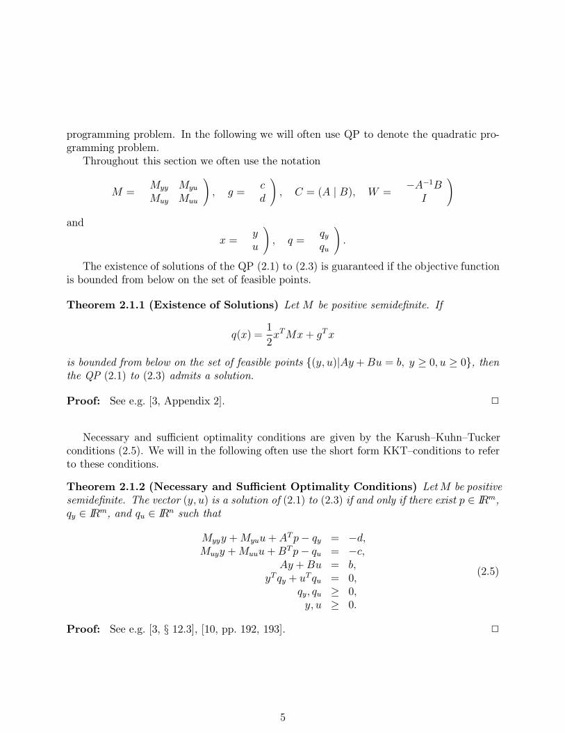
Throughout this section we often use the notation

M =

(Myy Myu

Muy Muu

), g =

(cd

), C = (A | B), W =

(−A−1B

I

)

and

x =

(yu

), q =

(qyqu

).

The existence of solutions of the QP (2.1) to (2.3) is guaranteed if the objective functionis bounded from below on the set of feasible points.

Theorem 2.1.1 (Existence of Solutions) Let M be positive semidefinite. If

q(x) =1

2xTMx+ gTx

is bounded from below on the set of feasible points (y, u)|Ay+Bu = b, y ≥ 0, u ≥ 0, thenthe QP (2.1) to (2.3) admits a solution.

Proof: See e.g. [3, Appendix 2]. 2

Necessary and sufficient optimality conditions are given by the Karush–Kuhn–Tuckerconditions (2.5). We will in the following often use the short form KKT–conditions to referto these conditions.

Theorem 2.1.2 (Necessary and Sufficient Optimality Conditions) LetM be positivesemidefinite. The vector (y, u) is a solution of (2.1) to (2.3) if and only if there exist p ∈ IRm,qy ∈ IRm, and qu ∈ IRn such that

Myyy +Myuu+ATp− qy = −d,Muyy +Muuu+BTp− qu = −c,

Ay +Bu = b,yTqy + uTqu = 0,

qy, qu ≥ 0,y, u ≥ 0.

(2.5)

Proof: See e.g. [3, § 12.3], [10, pp. 192, 193]. 2

5

2.2 Interior–Point Methods for the Solution of the Quadratic

Programming Problem

In the presence of bound constraints (2.3) interior–point methods, in particular primal–dualNewton interior–point algorithms are very attractive methods for the solution of large–scale QPs. Unlike active set methods, which usually move along the boundary of the set(y, u) | y ≥ 0, u ≥ 0, interior–point methods, as suggested by the name, generate iterates(y, u) that are in the interior, i.e. satisfy y > 0, u > 0. This property allows interior–pointmethods to generate iterates that cut through the feasible set and move towards an optimumrather than exchanging one active index at a time and marching along the boundary towardsan optimum. In many cases, this property allows one to prove polynomial complexity ofinterior–point methods. See e.g. [17] for an overview of interior–point methods. We willsketch primal–dual Newton interior–point methods and barrier methods for the solution ofthe QP (2.1) to (2.3).

We will employ the notation usual in interior–point methods: For a given vector x, thediagonal matrix with diagonal entries equal to the entries of x is denoted by X. Throughoutthis section, e denotes the vector of ones: e = (1, . . . , 1).

The construction of primal–dual Newton interior–point is based on the so–called per-turbed KKT conditions corresponding to (2.5), which are given by

Mx+ CTp− q = −g,Cx = b,

XQe = θe,(2.6)

and x, q > 0, where θ > 0. To move from a current iterate (x, p, q) with x, q > 0 to the nextiterate (x+, p+, q+), primal–dual Newton interior–point methods compute the Newton step(∆x,∆p,∆q) for the perturbed KKT conditions (2.6) and set

(x+, p+, q+) = (x+ αx∆x, p+ αp∆p, q + αq∆q),

where the step sizes αx, αp, αq ∈ (0, 1] are chosen so that x+, q+ > 0. Then the perturbationparameter θ is updated based on xT+q+ and the previous step is repeated. We refer to theliterature, e.g. [4], [17], [18], for details. We will focus on the relation of the Newton systemwith the system (1.1) under consideration.

The Newton system for the perturbed KKT–conditions (2.6) is given by M CT −IC 0 0Q 0 X

∆x

∆p∆q

= −

Mx+ CTp− q + gCx− b

XQe− θe

. (2.7)

The nonsymmetric system (2.7) can be reduced to a symmetric system. If we use the lastequation in (2.7) to eliminate ∆q,

∆q = −X−1Q∆x−Qe+ θX−1e (2.8)

6

then we arrive at the system M +X−1Q CT

C 0

∆x

∆p

= − Mx + CTp+ g − θX−1e

Cx− b

(2.9)

or, using the original notation, Myy + Y −1Qy Myu AT

Muy Muu + U−1Qu BT

A B 0

∆y

∆u∆p

= −

Myyy +Myuu+ATp+ c− θY −1eMuyy +Muuu+BTp + d− θU−1e

Ay +Bu− b

.(2.10)

If Myu = 0,Muy = 0, the system (2.10) is of the form (1.1). As variables yj or ui approachthe bound, i.e. approach zero, large quantities are added to the diagonals (j, j) or (i, i),respectively. In actual computations more care must be taken during the reduction of thesystem (2.7) to avoid cancellation in the reduction process due to very large elements in X−1,see e.g. [5]. A stable reduction of the system (2.7) is discussed in [5]. The unknowns andthe right hand side in that reduced system differ from those in (2.10). However, the systemmatrix in the stable reduction is equal to the system matrix in (2.10). For our purposes itis therefore not necessary to present the lengthier stable reduction and we refer to [5] fordetails.

For completeness we also mention barrier methods for the solution of the QP (2.1) to(2.3). In a barrier method with logarithmic barrier function, one generates a sequence ofiterates (y, u, p) with y > 0, u > 0 by approximately minimizing

Minimize1

2

(yu

)T (Myy Myu

Muy Muu

)(yu

)+

(cd

)T (yu

)− µ

m∑i=1

ln(yi)− µn∑i=1

ln(ui)

(2.11)subject to

Ay +Bu = b (2.12)

and y, u > 0. During the iteration, the positive barrier parameter µ is adjusted so thatµ → 0. The minimization is performed by Newton’s method. The KKT conditions for theproblem (2.11), (2.12) are given by

Mx− µX−1e+ CTp = −g,Cx = b.

(2.13)

The Newton system for (2.13) is given by(M + µX−2 CT

C 0

)(∆x∆p

)= −

(Mx− µX−1e+ CTp + g,

Cx− b.

). (2.14)

If Myu = 0,Muy = 0, the system (2.14) is of the form (1.1). As before, large quantities areadded to the diagonals (j, j) or (i, i), as variables yj or ui approach the bound, i.e. approachzero, respectively. For more details on the barrier method we refer to [17]. For a discussion ofthe relation, in particular the differences, between barrier methods and primal–dual Newtoninterior–point methods see [4].

7

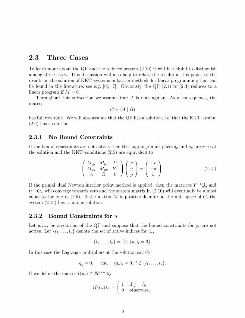
2.3 Three Cases

To learn more about the QP and the reduced system (2.10) it will be helpful to distinguishamong three cases. This discussion will also help to relate the results in this paper to theresults on the solution of KKT–systems in barrier methods for linear programming that canbe found in the literature, see e.g. [6], [7]. Obviously, the QP (2.1) to (2.3) reduces to alinear program if M = 0.

Throughout this subsection we assume that A is nonsingular. As a consequence, thematrix

C = (A | B)

has full row rank. We will also assume that the QP has a solution, i.e. that the KKT–system(2.5) has a solution.

2.3.1 No Bound Constraints

If the bound constraints are not active, then the Lagrange multipliers qy and qu are zero atthe solution and the KKT–conditions (2.5) are equivalent to Myy Myu AT

Muy Muu BT

A B 0

yup

=

−c−db

. (2.15)

If the primal–dual Newton interior–point method is applied, then the matrices Y −1Qy andU−1Qu will converge towards zero and the system matrix in (2.10) will eventually be almostequal to the one in (2.5). If the matrix M is positive definite on the null–space of C, thesystem (2.15) has a unique solution.

2.3.2 Bound Constraints for u

Let y∗, u∗ be a solution of the QP and suppose that the bound constraints for y∗ are notactive. Let l1, . . . , lk denote the set of active indices for u∗,

l1, . . . , lk = i | (u∗)i = 0.

In this case the Lagrange multipliers at the solution satisfy

qy = 0, and (qu)i = 0, i /∈ l1, . . . , lk.

If we define the matrix I(u∗) ∈ IRk×n by

(I(u∗))ij =

1 if j = li,0 otherwise,

8

then the KKT conditions (2.5) are equivalent toMyy Myu AT 0Muy Muu BT I(u∗)T

A B 0 00 I(u∗) 0 0

yupqau

=

−c−db0

, (2.16)

where qau denotes the Lagrange multipliers corresponding to the active indices. Since A isnonsingular, the matrix

C =

(A B0 I(u∗)

)has full row rank. Therefore, the system (2.16) is uniquely solvable, provided the matrix Mis positive definite on the null-space of C.

If M = 0, then the QP reduces to an LP. In this case the solution of the optimizationproblem can be found in a vertex. The columns of C = (A | B) corresponding to thepositive components of the vertex (y∗, u∗) are linearly independent, see e.g. [3, § 2]. Since,by assumption, y∗ > 0 and A is nonsingular, we can conclude that u∗ = 0. Consequently,I(u∗) ∈ IRn×n is the identity matrix. In the language of linear programming, y∗ are the basisvariables and u∗ are the nonbasis variables. Thus, we have exactlym positive basis variables.This case is called the nondegenerate case in linear programming.

It has been observed, e.g. [6], [7], that in the nondegenerate case the KKT systems inbarrier methods for linear programming can be preconditioned effectively. This will also betrue in our case. If only bounds on u are active, efficient preconditioners can be constructedfor the problems investigated in this paper. However, in our applications, ill–conditioningalso arises from the matrices A. Although proven to be nonsingular, the matrices A arisingin our applications have a wide spectrum which causes a large spread in the spectrum of theKKT matrix K. This will be investigated in more detail in Section 6.

2.3.3 Bound Constraints for u and y

Let y∗, u∗ be a solution of the QP. Furthermore, let lu1 , . . . , luku denote the set of activeindices for u∗,

lu1 , . . . , luku = i | (u∗)i = 0and let ly1 , . . . , lyky denote the set of active indices for y∗,

ly1, . . . , lyky = i | (y∗)i = 0.

In this case the Lagrange multipliers at the solution satisfy

(qy)i = 0, i /∈ ly1, . . . , lyky and (qu)i = 0, i /∈ lu1 , . . . , luku.

If we define the matrices I(y∗) ∈ IRky×m, I(u∗) ∈ IRku×n by

(I(y∗))ij =

1 if j = lyi ,0 otherwise,

and (I(u∗))ij =

1 if j = lui ,0 otherwise,

9

then the KKT conditions (2.5) are equivalent toMyy Myu AT I(y∗)T 0Muy Muu BT 0 I(u∗)T

A B 0 0 0I(y∗) 0 0 0 0

0 I(u∗) 0 0 0

yupqayqau

=

−c−db00

, (2.17)

where qay , qau denote the Lagrange multipliers corresponding to the active indices.

The assumption that A is nonsingular is not sufficient to guarantee that the matrix

C =

A BI(y∗) 0

0 I(u∗)

(2.18)

has full row rank. If C does not have full rank, then the system (2.17) does not have aunique solution. In fact, in this case there exists (δp, δqay , δq

au) 6= (0, 0, 0) with

(AT I(y∗)T 0BT 0 I(u∗)T

) δpδqayδqau

=

(00

),

and, thus,Myy Myu AT I(y∗)T 0Muy Muu BT 0 I(u∗)T

A B 0 0 0I(y∗) 0 0 0 0

0 I(u∗) 0 0 0

yu

p + tδpqay + tδqayqau + tδqau

=

−c−db00

∀ t ∈ IR.

Thus, in this case the Lagrange multipliers (p, qay , qau) are not uniquely determined.

If M = 0, then the QP reduces to an LP and the solution of the optimization problemcan be found in a vertex (y∗, u∗). In this case the columns of C = (A | B) correspondingto the positive components of the vertex (y∗, u∗) are linearly independent. Thus, at most mcomponents of (y∗, u∗) can be positive. If less than m components of (y∗, u∗) are positive thevertex is called degenerate, see e.g. [3, § 2].

In the nondegenerate case, i.e. if m components of (y∗, u∗) are positive, then we can finda column permutation Π for the matrix C defined in (2.18) such that

C Π =

A BI(y∗) 0

0 I(u∗)

Π =

(CB CN0 I

),

where CB ∈ IRm×m is the nonsingular basis matrix and I ∈ IRn×n denotes the identity. Thisshows that in the nondegenerate case the matrix C has full row rank. In the degenerate

10

case, however, l < m components of (y∗, u∗) are positive. Thus,

C =

A BI(y∗) 0

0 I(u∗)

∈ IR(m+(m+n−l))×(m+n)

and 2m+ n− l > m+ n. Hence, the matrix C cannot have full row rank.This shows that the degenerate case occurs if and only if C does not have full row rank.For the construction of preconditioners in barrier methods for linear programming the

degenerate case is the difficult one. For example, the preconditioners discussed in [6], arefar less effective in reducing the condition number of the KKT matrix in the degeneratecase than they are in the nondegenerate case, cf. Tables 1 and 2 in [6]. Unfortunately, butnot surprisingly this will also be the case in our situation. If bounds are only imposed onthe controls u, efficient and rather general preconditioners can be derived. However, if stateconstraints, i.e. bounds on y, are present and active, then the design of preconditioners ismuch more difficult. We will investigate this in detail in Section 6.

11

Chapter 3

Eigenvalue Estimates

The eigenvalue distribution of the Karush–Kuhn–Tucker system is of great importance forthe iterative solution methods we use. The convergence of MINRES and SYMMLQ dependsmainly on the eigenvalue distribution of the system.

First we will study the numbers of positive, negative and zero eigenvalues of

K =

Hy 0 AT

0 Hu BT

A B 0

, (3.1)

then we estimate the eigenvalues of the entire system by the eigenvalues and singular valuesof the constituting submatrices.

We assume that A is invertible, and we use the notation

H =

(Hy 00 Hu

), C = (A | B), W =

(−A−1B

I

).

3.1 The Eigenvalue Distribution

To find out about the eigenvalue distribution of K, we apply congruence transformations.From the decomposition I 0 0

−(A−1B)T I 00 0 A−1

Hy 0 AT

0 Hu BT

A B 0

I −A−1B 0

0 I 00 0 A−T

=

Hy (Hy| 0) W I

W T(Hy0

)W TH W 0

I 0 0

(3.2)

12

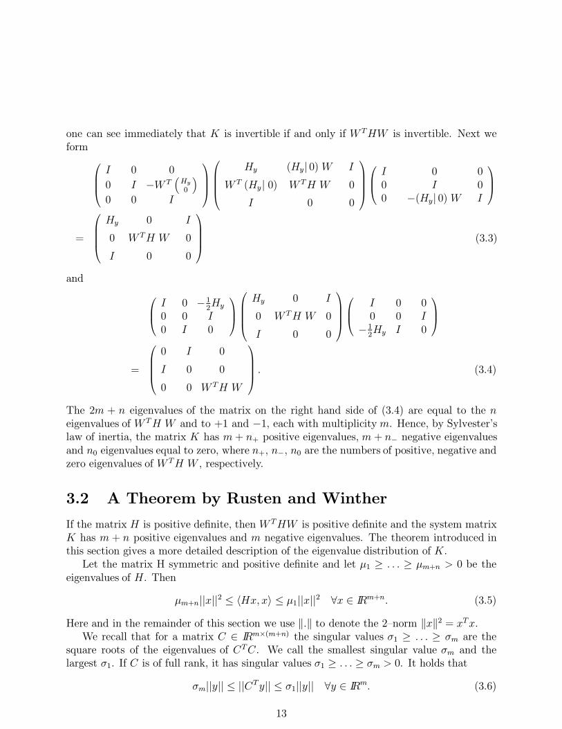
one can see immediately that K is invertible if and only if W THW is invertible. Next weform

I 0 0

0 I −W T(Hy0

)0 0 I

Hy (Hy| 0) W I

W T (Hy | 0) W TH W 0

I 0 0

I 0 0

0 I 00 −(Hy| 0) W I

=

Hy 0 I

0 W TH W 0

I 0 0

(3.3)

and I 0 −12Hy

0 0 I0 I 0

Hy 0 I

0 W TH W 0

I 0 0

I 0 0

0 0 I−1

2Hy I 0

=

0 I 0

I 0 0

0 0 W TH W

. (3.4)

The 2m + n eigenvalues of the matrix on the right hand side of (3.4) are equal to the neigenvalues of W TH W and to +1 and −1, each with multiplicity m. Hence, by Sylvester’slaw of inertia, the matrix K has m+ n+ positive eigenvalues, m + n− negative eigenvaluesand n0 eigenvalues equal to zero, where n+, n−, n0 are the numbers of positive, negative andzero eigenvalues of W TH W , respectively.

3.2 A Theorem by Rusten and Winther

If the matrix H is positive definite, then W THW is positive definite and the system matrixK has m + n positive eigenvalues and m negative eigenvalues. The theorem introduced inthis section gives a more detailed description of the eigenvalue distribution of K.

Let the matrix H symmetric and positive definite and let µ1 ≥ . . . ≥ µm+n > 0 be theeigenvalues of H. Then

µm+n||x||2 ≤ 〈Hx, x〉 ≤ µ1||x||2 ∀x ∈ IRm+n. (3.5)

Here and in the remainder of this section we use ‖.‖ to denote the 2–norm ‖x‖2 = xTx.We recall that for a matrix C ∈ IRm×(m+n) the singular values σ1 ≥ . . . ≥ σm are the

square roots of the eigenvalues of CTC. We call the smallest singular value σm and thelargest σ1. If C is of full rank, it has singular values σ1 ≥ . . . ≥ σm > 0. It holds that

σm||y|| ≤ ||CTy|| ≤ σ1||y|| ∀y ∈ IRm. (3.6)

13

andσm||x|| ≤ ||Cx|| ≤ σ1||x|| ∀x ∈ N(C)⊥ (3.7)

Note that this implies that the right inequality holds for all x ∈ IRm+n.

For a system matrix of this structure, the following result holds which is taken from [14]:

Theorem 3.2.1 Let µ1 ≥ µ2 ≥ . . . ≥ µm+n > 0 be the eigenvalues of H, let σ1 ≥ . . . ≥σm > 0 be the singular values of CT . The eigenvalues λ1 ≥ . . . ≥ λm+n > 0 > λm+n+1 ≥. . . ≥ λ2m+n of K satisfy

λ2m+n ≥1

2(µm+n −

√µ2m+n + 4σ2

1), (3.8)

λm+n+1 ≤1

2(µ1 −

õ2

1 + 4σ2m), (3.9)

λm+n ≥ µm+n, (3.10)

λ1 ≤1

2(µ1 +

õ2

1 + 4σ21). (3.11)

Proof: Let λ ∈ Λ(K) and let (x, y) be the corresponding eigenvector, i.e.

Hx+ CTy = λx, (3.12)

Cx = λy. (3.13)

Note that if x = 0, then y = 0 by (3.13). This is not admissible for an eigenvector (x, y).Hence x 6= 0.

1. First we bound the positive eigenvalues. Let λ be a positive eigenvalue of K. Combin-ing the inner product of (3.12) with x and the inner product of (3.13) with y yields

xTHx+ λ||y||2 = λ||x||2.

Since by (3.5)µm+n||x||2 ≤ xTHx = λ||x||2 − λ||y||2,

we have(µm+n − λ)||x||2 ≤ −λ||y||2 ≤ 0,

and thusλ ≥ µm+n.

To derive an upper bound, use (3.13) in the form y = 1λCx and the inner product of

(3.12) with x to obtain

xTHx+1

λxTCTCx = λ||x||2.

14

Using (3.5) and (3.7) we derive the inequality

(λ2 − µ1λ− σ21)||x||2 ≤ 0.

The roots of λ2 − µ1λ− σ1 = 0 are 12(µ1 ±

õ2

1 + 4σ21).

Since ||x||2 is positive, we conclude

λ ≤ 1

2(µ1 +

õ2

1 + 4σ21).

2. Now consider a negative eigenvalue λ of K.

The derivation of a lower bound for the negative eigenvalues is similar to the derivationof the upper bound for the positive eigenvalues.

To derive an upper bound for the negative eigenvalues, let x = v+w, where v ∈ N(C)⊥

and w ∈ N(C). Taking the inner product of (3.12) with v and substituting y from (3.13)into this expression we get, using orthogonality,

vTHw = −vTHv − 1

λ||Cv||2 + λ||v||2.

Using the bounds (3.5) and (3.7) we obtain

vTHw ≥ (λ− µ1 −1

λσ2m)||v||2. (3.14)

To proceed, we must find a bound for vTHw. This is achieved by taking the innerproduct of (3.12) with w and using (3.5). Since w ∈ N(C)⊥ we get

wTHx+ wTCTy = wTHv + wTHw = λwTx = λwTw.

Thus with λ− µm+n < 0 this implies

wTHv ≤ (λ− µm+n)||w||2 ≤ 0.

Together with (3.14) and the symmetry of H we obtain

0 ≥ (λ− µ1 −σ2m

λ)||v||2, and thus 0 ≤ (λ2 − µ1λ− σ2

m)||v||2.

If v = 0, (3.13) implies y = 0 and (3.12) reduces to Hw = λw. Since λ is negative andH positive definite, this is a contradiction. It follows that (λ2−µ1λ−σ2

m) ≥ 0, leadingto the final estimate

λ ≤ 1

2(µ1 −

õ2

1 + 4σ2m).

2

15

Chapter 4

SYMMLQ AND MINRES

4.1 Introduction to SYMMLQ and MINRES

The Karush–Kuhn–Tucker systems we want to solve are of the form Hy 0 AT

0 Hu BT

A B 0

yup

=

cdb

, (4.1)

where Hy and Hu are symmetric.In our applications, the system matrix is very large and sparse. Usually we only compute

the blocks and do not really assemble them into an entire system matrix. Therefore we wantto use iterative solvers that only require matrix–vector products. Moreover, the matricesin our applications are not always explicitly known. Only their action on vectors can becomputed, so that an iterative approach may even be the only appropriate way to handlethe arising systems.

An effective and popular method for symmetric positive definite systems is the conjugategradient method. However, since the system matrix in (4.1) is symmetric indefinite, theconjugate gradient method is not applicable. For symmetric indefinite systems Paige andSaunders [13] have derived two iterative methods, MINRES and SYMMLQ, which can beviewed as generalizations of the conjugate gradient method for the solution of indefinitesystems. These methods will introduced and analyzed in this chapter.

In this chapter we do not use the notation (4.1), but the notation generally used for linearsystems. Instead of (4.1) we consider

Ax = b, (4.2)

where A ∈ IRn×n is symmetric indefinite.We use the notation

‖x‖ = ‖x‖2 =√xTx and 〈x, y〉 = xTy.

The presentation in this chapter closely follows [9].

16

4.2 Derivation of SYMMLQ and MINRES

An iterative method for the solution of symmetric positive definite linear systems, suitablefor large and sparse problems

Ax = b (4.3)

is the conjugate gradient method. MINRES and SYMMLQ are generalizations of the con-jugate gradient method for the symmetric indefinite case. Because SYMMLQ and MINRESare closely related to the conjugate gradient method, we give a brief introduction to theconjugate gradient method.

The derivation of the conjugate gradient method can be based on the fact that for positivedefinite matrices A the problem (4.3) is equivalent to the minimization problem

minx∈IRn

F (x) =1

2〈x,Ax〉 − 〈x, b〉. (4.4)

In the positive definite case, the minimization problem has a unique solution. The minimizeris x = A−1b. This makes (4.4) and (4.3) interchangeable.

By construction of the method, the conjugate gradient method really solves

Ax = r0, (4.5)

where r0 is the initial residual r0 = b − Ax0. We do not want to assume that our startingvector is x0 = 0. If x0 6= 0 is a more appropriate initial guess, we apply the conjugategradient method to (4.3) with b replaced by r0 = b − Ax0. Equally, we write (4.4) in theform

minx∈IRn

F (x) =1

2〈x,Ax〉 − 〈x, r0〉. (4.6)

The starting point in the derivation of the conjugate gradient method is to consider howone one might go about minimizing the functional F in (4.6). A classical approach is thesteepest descent or gradient method. Because of symmetry of A, the gradient of F is givenby

∇F (x) = Ax− r0.

If the gradient is nonzero there exists a positive scalar α such that

F (x− α∇F (x)) < F (x).

We now adopt an iterative point of view. Given the iterate xj in step j we take the directionof the negative gradient to get to the next iterate

xj+1 = xj − αj∇F (xj) = xj − αj(Axj − r0) = xj − αjrj,

where rj = Axj − r0 denotes the residual in iteration j. We choose the step size α such thatF is minimized along the step. The solution is

αj =〈rj, Axj − r0〉〈rj, Arj〉

.

17

With this choice, the ’exact step size’, a drawback of the gradient method becomesapparent. It holds that successive gradients and steps are orthogonal. This usually leads tounsatisfactory convergence behavior of the gradient method. The reason is that we computea new iterate that is optimal with respect to the search direction rj, but not with respect tothe previously used search directions.

Nevertheless, we do not totally discard this choice of a search direction. Our goal nowis to construct a method which preserves the optimality with respect to previously useddirections and that effects improvement in the minimization problem (4.6).

We say that xj ∈ spanp0, . . . , pj is optimal with respect to p0, . . . , pj if

〈Axj − r0, v〉 = 0 ∀v ∈ spanp0, . . . , pj. (4.7)

If p0, . . . , pj−1 are search directions from the previous iterations and if xj is the currentiterate, optimal with respect to spanp0, . . . , pj−1, then we want to construct a new iteratexj+1 with the help of a new search direction pj such that if we take the exact step sj = αjpj,the new iterate is optimal with respect to pj and to spanp0, . . . , pj−1, i.e. we want pj , xj+1

such thatF (xj+1) = min

x∈spanp0,...,pj−1,pjF (x).

Using the optimality of xj with respect to spanp0, . . . , pj−1, we find that for i = 0, . . . , j−1

0 = 〈Axj+1 − r0, pi〉= 〈A(xj + αjpj)− r0, pi〉= 〈Axj − r0, pi〉+ αj〈Apj , pi〉 (4.8)

= αj〈Apj , pi〉.

The property 〈Apj , pi〉 = 0, i 6= j, is the A–orthogonality of pj with respect to the directionsp0, . . . , pj−1. So we have to search for a vector pj that is A–orthogonal to p0,. . . ,pj−1 in orderto get a new search direction.

If we are given A–orthogonal pi, i = 0, . . . , j − 1, and a current iterate xj that is optimalwith respect to the span of these search directions, then we can take the negative gradientas a descent direction and modify it in order to suffice the additional requirement. Using theGram–Schmidt Orthogonalization we construct pj from rj in subtracting those componentsof rj that are not A–orthogonal to the previous directions pi.

Suppose we have pi, i = 0, . . . , j − 1, such that 〈pi, Api〉 6= 0, i = 0, . . . , j − 1, and〈pi, Apk〉 = 0 for k 6= i, i, k = 0, . . . , j − 1, then

pj = rj −j−1∑i=0

〈rj , Api〉〈pi, Api〉

pi

is A–orthogonal to p0, . . . , pj−1. One can show that

spanp0, . . . , pi = spanr0, . . . , ri = spanr0, Ar0, . . . , Air0 = Ki+1(A, r0).

18

We have then Api ∈ spanr0, . . . , Ai+1r0 = spanp0, . . . , pi+1. Since xj is optimal withrespect to spanp0, . . . , pi−1 we get 〈rj , Api〉 = 0 for i = 0, 1, . . . , i− 2. Hence

pj = rj −〈rj , Apj−1〉〈pj−1 , Apj−1〉

pj−1.

The requirement that xj+1 is optimal with respect to pj yields

αj =〈rj, pj〉〈Apj , pj〉

=‖rj‖2

〈Apj , pj〉,

see (4.8) with i = j. The identity 〈rj , pj〉 = ‖rj‖2 follows from the construction of pj .In each step the conjugate gradient method computes the iterate xk in the Krylov sub-

spaceKk(A, r0) = spanr0, Ar0, . . . , A

k−1r0which minimizes F overKk(A, r0), i.e. the iterate xk solves (4.6). Problem (4.6) is equivalentto (4.7), i.e. to solving

〈Axk − r0, v〉 = 0 ∀v ∈ Kk(A, r0). (4.9)

The conjugate gradient method minimizes the error in the A–norm ‖.‖A. This norm isfor symmetric positive definite matrices A defined by ‖x‖A = xTAx. The minimization of‖e‖A follows from the identity

F (xj) = minx∈Kj(A,r0)

F (x)

= minx∈Kj(A,r0)

1

2〈x,Ax〉 − 〈x, r0〉

= minx∈Kj(A,r0)

1

2〈x,Ax〉 − 2〈x,Ax∗〉 + 〈x∗, Ax∗〉

= minx∈Kj(A,r0)

1

2〈x∗ − x,A(x∗ − x)〉

= minx∈Kj(A,r0)

1

2‖e‖A. (4.10)

If A is not positive definite, then (4.5) and (4.6) are not equivalent. In fact, (4.6) does nothave a solution if A has negative eigenvalues, and it may not have a solution if A is onlypositive semidefinite. Even though in this case the foregoing derivation is not applicable,one can try to extend the conjugate gradients method by trying to compute the iterates xkas a solution of (4.9). This leads to SYMMLQ.

SYMMLQ tries to compute the iterate xk ∈ Kk(A, r0) such that xk solves

〈r0 − Axk, v〉 = 0 ∀v ∈ Kk(A, r0). (4.11)

The vector xk ∈ Kk(A, r0) is called a Galerkin approximation to the solution x∗ of Ax = bover the Krylov subspace Kk(A, r0).

19

Unfortunately, (4.11) need not have a solution. Consider the following example:If

r0 =

(10

), A =

(0 11 1

),

then

K1(A, r0) = spanr0 =

(α0

): α ∈ IR

.

We have then with x = (x1, 0)T , v = (v1, 0)T ∈ K1(A, r0)

〈r0 −Ax, r0〉 = (1,−x1)T (v1, 0) = v1 6= 0

in general, so that the Galerkin approximation problem does not have a solution.

This is the reason why SYMMLQ uses a slightly different iterate which is derived fromthe implementation of this method and will be discussed in detail in Section 4.4. If A ispositive definite, then (4.9) has a unique solution, and SYMMLQ is equivalent to the methodof conjugate gradients. In this case, SYMMLQ minimizes the error ‖ej‖A in each step.

An alternative is MINRES. It is based on another approximation to the exact solution.In iteration k, k = 0, 1, . . ., MINRES computes xk ∈ Kk(A, r0) such that xk solves

minx∈Kk(A,r0)

‖r0 − Ax‖. (4.12)

This definition of an approximation is motivated by the use of the residual Axk − r0 asa measure for the closeness of the current iterate and the exact solution. The vector xk iscalled a minimum residual approximation to the solution x∗ of Ax = r0. The least squaresproblem (4.12) always has a unique solution. This will be shown in Theorem 4.4.5.

The implementation of SYMMLQ and MINRES will be discussed in Section 4.4.

4.3 Convergence Analysis

MINRES and SYMMLQ are, like the conjugate gradient method, n–step prodecures. Theirfinite termination will be established here. However, rounding errors may lead to a loss oforthogonality among theoretically orthogonal vectors and finite termination is not mathe-matically guaranteed. Moreover, when these iterative solvers are applied, n is usually sobig that O(n) iterations represent an unacceptable amount of work. As a consequence, it iscustomary to regard the methods as genuinely iterative techniques with termination basedupon an iteration maximum and the residual norm. With this point of view, the rate ofconvergence becomes important.

The convergence of Krylov subspace methods is related to properties of uniform bestapproximating polynomials. This relation is based on the fact that vectors in Krylov sub-spaces have a special representation. This representation will now be derived. We need thefollowing notation.

20

Let Πk denote the space of all polynomials of degree k or less, and Π1k the space of all

polynomials of degree k or less that are one at the origin, i.e.

Π1k = p ∈ Πk | p(0) = 1.

Recall that we use the 2–norm, i.e. ‖.‖ always means ‖.‖2.

Theorem 4.3.1 Let A ∈ IRn×n and let v ∈ IRn. Let Πk denote the space of polynomials ofdegree less or equal to k, then

Kk(A, v) = p(A)v | p ∈ Πk−1.

Proof: Let x ∈ Kk(A, v). Then x is a linear combination of v, Av, . . . , Ak−1v, i.e. thereare scalars αi ∈ IR , i = 0, . . . , k− 1, such that

x = α0v + α1Av + . . .+ αk−1Ak−1v =

k−1∑i=0

αiAiv = p(A)v

for the polynomial p defined by these coefficients. Clearly p ∈ Πk−1. Conversely, if x = p(A)vfor a polynomial p ∈ Πk−1, then x is an element of the Krylov subspace as a linear combi-nation of the basis vectors v, Av, . . . , Ak−1v. 2

We consider Krylov subspace methods solving the problem

Ax = r0

with r0 = Ax0 − b. However, we are interested in solutions x∗ of the problems Ax = b. Thiscorresponds to a variable transformation xk + x0 → xk. If xk are the iterates generated bythe Krylov subspace methods satisfying xk ∈ Kk(A, r0), then xk + x0 ∈ x0 + Kk(A, r0). Weconsider vectors x satisfying x+ x0 ∈ x0 + Kk(A, r0).

Theorem 4.3.1 establishes that vectors in the Krylov subspace have a special representa-tion, and due to this representation we have that x+x0 = x0+pk−1(A)r0 for some polynomialpk−1 ∈ Πk−1 of degree less or equal to k− 1. With this representation for x we can write theresidual r(x) = b− A(x+ x0) in the form

r(x) = b− A(x+ x0) = b− Ax0 − Ax = r0 −Ax = (I − Apk−1(A))r0 = p1k(A)r0. (4.13)

The polynomial p1k = (1− pk−1(.)) is of degree less or equal to k and satisfies p1

k(0) = 1. Sowe write p1

k ∈ Π1k. Similarly, the error e(x) = x∗ − x0 − x can be written as

e(x) = x∗ − x0 − x = x∗ − x0 − pk−1(A)r0 = (I − pk−1(A)A)(x∗− x0) = p1k(A)e0. (4.14)

The polynomial p1k = (1− pk−1(.)) in the representation of the residual is the same as in the

representation of the error.

21

If we consider the iterates xk, we write

rk = r(xk) = b− A(xk + x0)

andek = e(xk) = x∗ − (xk + x0).

The conjugate gradient method and its generalizations, MINRES and SYMMLQ, iterateon Krylov subspaces of increasing dimension that eventually are invariant subspaces of thesystem matrix A. One of the features these methods have in common is the finite conver-gence. This feature, obvious by construction of the subspace and the linear independence ofthe basis vectors, will now be formally shown.

Theorem 4.3.2 Let A ∈ IRn×n be nonsingular. Then there exists a polynomial p ∈ Πn−1

such thatA−1 = p(A).

Proof: The Hamilton–Cayley Theorem says that a matrix annihilates its own characteristicpolynomial, i.e. if A ∈ IRn×n and if pA(λ) = det(A−λI) denotes the characteristic polynomialof A, then

pA(A) = 0.

From this we can conclude the following: If pA(λ) =∑ni=0 aiλ

i, then a0 6= 0 if and only ifA is nonsingular, i.e. if λ = 0 is not an eigenvalue of A. In this case, we find that

I = A(−a−10

n∑i=1

aiAi−1).

Hence,

A−1 = −a−10

n∑i=1

aiAi−1

and we know that there exists a polynomial pn−1 of degree less or equal to n−1 such that theinverse of A can be written as a polynomial in A: A−1 = pn−1(A). In particular we obtain

A−1r0 = pn−1(A)r0.

2

If Akr0 ∈ Kk(A, r0) for some k, then Alr0 ∈ K(A, r0) for all l ≥ k. This meansthat we have encountered an invariant subspace for A. This implication will be shownin Lemma 4.3.4. The solution to Ax = r0 can be found in this subspace which is in the worstcase encountered for k = n, in more favorable circumstances for k n. From this we canconclude that there exists a polynomial pk−1 of degree less or equal to k − 1 such that

A−1r0 = pk−1(A)r0. (4.15)

22

Before investigating more specialized results concerning the convergence of the minimumresidual approximations, we state the result on the finite termination of Krylov minimumresidual methods.

Theorem 4.3.3 Let A ∈ IRn×n be a nonsingular matrix. If xk are minimum residual ap-proximations of x∗ on Kk(A, r0), then there exists k∗ ≤ n such that the residual rk∗ = b−Ax∗satisfies

‖rk∗‖ = 0.

Proof: From Theorem 4.3.2 we know that there exists a polynomial pk∗−1 of degree less orequal to k∗−1 ≤ n−1, such that x∗−x0 = A−1r0 = pk∗−1(A)r0 and so r0−Apk∗−1(A)r0 = 0.Hence,

‖rk∗‖ = minp∈Π1

k∗

‖p(A)r0‖ ≤ ‖(I − Apk∗−1(A))r0‖ = 0.

2

Likewise, we can show finite convergence for the Galerkin approximations. The previousproof relies on the minimization property of the MINRES iterates. Because SYMMLQ doesnot minimize the residual, we have to use another approach.

In the following lemma it will be shown that Krylov subspaces of maximal dimension areinvariant subspaces for the generating matrix. This means that if Ak ∈ Kk(A, v), then

A(Kl(A, v)) ⊂ Kk(A, v) ∀l ≥ k.

Lemma 4.3.4 If Akv ∈ Kk(A, v), then Alv ∈ Kk v for all l ≥ k.

Proof: The proof can be done by induction. Here only the actual induction step

Akv ∈ Kk(A, v) =⇒ Ak+1v ∈ Kk(A, v)

will be done. Since we know from Theorem 4.3.1 that Akv ∈ Kk(A, v) if and only if it hasa representation

Akv =k−1∑j=0

αjAjv,

for some scalars αj ∈ IR, we find by applying such a representation twice that

Ak+1v = AAkv =k−1∑j=0

ajAAjv =

k−2∑j=0

ajAj+1v + ak−1

k−1∑j=0

ajAjv ∈ Kk(A, v).

2

23

Theorem 4.3.5 Let A ∈ IRn×n be a nonsingular matrix. Suppose that the Galerkin ap-proximations xk of x∗ on Kk(A, r0) exist. Then there exists k∗ ≤ n such that the residualrk∗ = r0 − Ax∗ satisfies

rk∗ = 0.

Proof: For some k ∈ IN the Krylov subspace Kk(A, r0) is an invariant subspace for A, i.e.

∃ k ∈ IN : AKk(A, r0) ⊂ Kk(A, r0).

This is at least true for k = n, since Ki(A, r0) ⊂ IRn for all i. Suppose that Kk∗(A, r0) isan invariant subspace for A and that xk∗ ∈ Kk∗(A, r0) is the Galerkin approximation to thesolution x∗ of Ax = r0. Then by optimality we have

〈Axk∗ − r0, v〉 = 0 ∀v ∈ Kk∗(A, r0). (4.16)

Because of the invariance of Kk∗(A, r0) it holds

Axk∗ − r0 ∈ Kk∗(A, r0).

Using v = Axk∗ − r0 in (4.16) gives

‖Axk∗ − r0‖2 = ‖rk∗‖2 = 0.

2

4.3.1 Convergence Results for MINRES

The MINRES iterate xk satisfies ‖r0 −Axk‖ = minx∈Kk(A,r0) ‖r0 − Ax‖ and hence

‖rk‖ = ‖r0 − Axk‖ = ‖r0 − Apk−1(A)r0‖

for a polynomial pk−1 satisfying

‖rk‖ = ‖r0 − Apk−1(A)r0‖ = minp∈Πk−1

‖r0 − Ap(A)r0‖, (4.17)

or, equivalently,

‖rk‖ = ‖ r0 − Axk‖ = ‖r0 − Apk−1(A)r0‖ = ‖ p1k(A)r0 ‖

for a polynomial p1k ∈ Π1

k satisfying

‖ p1k(A)r0 ‖ = min

p∈Π1k

‖ p(A)r0 ‖.

24

Therefore we can use the norm of the residual rk = b − Axk to monitor the convergence ofMINRES.

Our main interest are symmetric indefinite system matrices. In this situation we will fromnow on use the following notation. If A ∈ IRn×n is nonsingular and symmetric indefinite,then all eigenvalues of A are contained in two intervals on the real line, one on the positive,one on the negative part. The spectrum is denoted by Λ(A) = Λ, and

Λ = [a, b] ∪ [c, d] for b < 0 < c

A set E ⊂ IR with the property E ⊃ Λ is called an inclusion set for the spectrum. Setting

λ = maxλ∈Λ|λ| and λ = min

λ∈Λ|λ|

we have [a, b] ⊂ [−λ,−λ], [c, d] ⊂ [λ, λ]. So, for example, E = [−λ,−λ]∪ [λ, λ] is an inclusionset. In addition to this, λi denotes the i–th largest eigenvalue, i.e.

λ1 ≥ . . . ≥ λl > 0 > λl+1 ≥ . . . ≥ λn.

Relation (4.17) and the minimization properties of MINRES imply the following result,see e. g. [15], [9], and for similar results for the conjugate gradient method see [1].

Theorem 4.3.6 Let A ∈ IRn×n be symmetric and Λ = λ1, . . . , λn denote its spectrum. Ifxk are minimum residual approximations to the solution of Ax = r0 on a Krylov sequence,then the following estimates hold for the corresponding residuals:

‖rk‖ ≤ minp∈Π1

k

maxi=1,...,n

|p(λi)| ‖r0‖, (4.18)

‖rk‖ ≤ minp∈Π1

2

maxi=1,...,n

|p(λi)| ‖rk−2‖. (4.19)

Proof: For symmetric matrices A there exists a similarity transformation such that A =V ΛV T where V is orthonormal and Λ is a diagonal matrix that contains the eigenvalues ofA.

Since V is orthonormal,

Aj = AA . . .A

= V ΛV TV ΛV T . . . V ΛV T

= V ΛΛ . . .ΛV T

= V ΛjV T

for all j ≥ 0. Thus p(A) = V p(Λ)V T holds for every polynomial p.

25

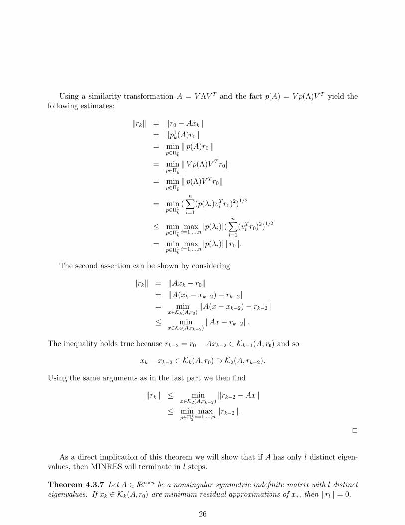
Using a similarity transformation A = V ΛV T and the fact p(A) = V p(Λ)V T yield thefollowing estimates:

‖rk‖ = ‖r0 −Axk‖= ‖p1

k(A)r0‖= min

p∈Π1k

‖ p(A)r0 ‖

= minp∈Π1

k

‖V p(Λ)V T r0‖

= minp∈Π1

k

‖ p(Λ)V Tr0‖

= minp∈Π1

k

(n∑i=1

(p(λi)vTi r0)2)1/2

≤ minp∈Π1

k

maxi=1,...,n

|p(λi)|(n∑i=1

(vTi r0)2)1/2

= minp∈Π1

k

maxi=1,...,n

|p(λi)| ‖r0‖.

The second assertion can be shown by considering

‖rk‖ = ‖Axk − r0‖= ‖A(xk − xk−2)− rk−2‖= min

x∈Kk(A,r0)‖A(x− xk−2)− rk−2‖

≤ minx∈K2(A,rk−2)

‖Ax− rk−2‖.

The inequality holds true because rk−2 = r0 − Axk−2 ∈ Kk−1(A, r0) and so

xk − xk−2 ∈ Kk(A, r0) ⊃ K2(A, rk−2).

Using the same arguments as in the last part we then find

‖rk‖ ≤ minx∈K2(A,rk−2)

‖rk−2 − Ax‖

≤ minp∈Π1

2

maxi=1,...,n

‖rk−2‖.

2

As a direct implication of this theorem we will show that if A has only l distinct eigen-values, then MINRES will terminate in l steps.

Theorem 4.3.7 Let A ∈ IRn×n be a nonsingular symmetric indefinite matrix with l distincteigenvalues. If xk ∈ Kk(A, r0) are minimum residual approximations of x∗, then ‖rl‖ = 0.

26

Proof: Let Λ = λ1, . . . , λl be the set of eigenvalues of A. The eigenvalues of A are theroots of the polynomial

p(x) =l∏

j=1

(1− x/λj),

which is of degree l. Since by (4.18) it holds

‖rl‖ ≤ minp∈Π1

l

maxi=1,...,n

|p(λi)| ‖r0‖ ≤ maxi=1,...,n

|p(λi)| ‖r0‖ = maxi=1,...,n

|l∏i=1

(1− λi/λj)| ‖r0‖ = 0,

we have the desired result. 2

Theorem 4.3.7 shows that the iterative process will stop after l steps if the system matrixhas l distinct eigenvalues. If this number l is small compared to the dimension of the system,we have a large computational gain. This result on its own already motivates preconditioning,which affects the eigenvalue distribution of the system matrix. Preconditioning will beintroduced in Section 5.

The convergence analysis of minimum residual approximations is closely related to theChebyshev approximation problem. We will therefore introduce briefly the Chebyshev ap-proximation problem and Chebyshev Polynomials. This presentation relies on [9] and [1].

Chebyshev Polynomials can be written in different forms. Consider first the function

Tk(cos θ) = cos(kθ), −π ≤ θ ≤ π.

Using the variable transformation x = cos(θ) we define for k ∈ IN0 the kth ChebyshevPolynomial Tk by

Tk = cos(k arccos(x)), x ∈ [−1, 1].

By the trigonometric identity

cos((k + 1)θ) = 2 cos(θ) cos(kθ)− cos((k − 1)θ)

we find that the Chebyshev Polynomials obey the three term recursion

T0(x) = 1, T1(x) = x, Tk+1(x) = 2xTk(x)− Tk−1(x), k = 2, 3, . . . (4.20)

This representation justifies the notion ’polynomial’. Moreover, this recursion can be used toextend the Chebyshev polynomials onto the whole real line. For every fixed x, the recursionin (4.20) has a characteristic equation λ2 = 2xλ− 1 whose roots are λ = x±

√x2 − 1. Using

these and the initial values T0(x) = 1, T1(x) = x, one finds that the Chebyshev Polynomialsare given by

Tk(x) =1

2

((x+

√x2 − 1)k + (x−

√x2 − 1)k

), k = 0, 1, . . . (4.21)

27

The problemminq∈Π1

k

maxx∈I|q(x)| (4.22)

for some closed and bounded interval I on the positive real line is a Chebyshev approximationproblem. For b > a > 0 the following result holds:

maxx∈[a,b]

|q∗k(x))| = minq∈Π1

k

maxx∈[a,b]

|q(x)|,

where

q∗k(x) = Tk

(b+ a− 2x

b− a

)/Tk

(b+ a

b− a

). (4.23)

The maximum is given by

maxx∈[a,b]

|q∗k(x)| =(Tk

(b+ a

b− a

))−1

. (4.24)

Here we require b > a > 0 because then we ascertain with b+ab−a > 1 that the denominator

in the definition of q∗k, Tk(b+ab−a), is not zero. This follows because all roots of the Chebyshev

Polynomial of order k, given by

x0i = cos

(2i− 1

k

π

2

), i = 1, . . . , k,

lie in [−1, 1]. Note that division by Tk(b+ab−a

)in the definition of q∗k normalizes it such that

q∗k ∈ Π1k.

Additionally, the following estimate of Tk(b+ab−a

)which will be used in Theorems 4.3.8,

4.3.9 and 4.3.10 holds. The estimate follows directly from the formulation (4.21). For k = 1it holds trivially

Tk

(b+ a

b− a

)=b+ a

b− a. (4.25)

For k > 1 we have from (4.21)

Tk

(b+ a

b− a

)=

1

2

(b+ a

b− a +2√ab

b− a

)k+

(b+ a

b− a −2√ab

b− a

)k=

1

2

((√a+√b)2

b− a

)k+

((√a−√b)2

b− a

)k=

1

2

√b/a+ 1√b/a− 1

k +

√b/a− 1√b/a+ 1

k

≥ 1

2

√b/a+ 1√b/a− 1

k , (4.26)

28

where the last inequality comes from the estimate c1 + c2 ≥ maxc1, c2 for positive realnumbers c1, c2.

With these tools we can now investigate convergence behavior of MINRES.The following standard convergence estimate can be found for example in [15].

Theorem 4.3.8 Let A ∈ IRn×n be a nonsingular, symmetric indefinite matrix. If xk ∈Kk(A, r0) are minimum residual approximations of x∗, then the residuals rk = r0−Axk obey

‖rk‖ ≤ 2(κ− 1

κ+ 1

)bk/2c‖r0‖,

where κ is the condition number of A given by κ = λ/λ. Here, λ = minλ∈Λ |λ|, λ =maxλ∈Λ |λ|, and bk/2c denotes the largest integer less or equal to k/2.

Proof: Knowing the result for the Chebyshev approximation problem we want to apply itto the recursion (4.18) already derived. To do this, we map the set [−λ,−λ]∪ [λ, λ], locatedon both sides of the origin, onto the interval [λ2, λ2] on the positive part of the real line.This is admissible since for p ∈ Π1

bk/2c the polynomial p(λ2) satisfies p(λ2) ∈ Π1k.

This established we find

‖rk‖/‖r0‖ ≤ minp∈Π1

k

maxλ≤|λ|≤λ

|p(λ)|

≤ minp∈Π1

bk/2c

maxλ≤|λ|≤λ

|p(λ2)|

≤ minp∈Π1

bk/2c

maxλ2≤λ≤λ2

|p(λ)|

=

(Tbk/2c

(κ2 + 1

κ2 − 1

))−1

≤ 2(κ− 1

κ + 1

)bk/2c.

The estimate follows from (4.26). 2

Considering the power bk/2c it is obvious that a decrease need not occur in every iteration.But it can be shown that a reduction in the residual is achieved at least after two iterations.

Theorem 4.3.9 Let A ∈ IRn×n be a nonsingular, symmetric indefinite matrix. If xk areminimum residual approximations on Kk(A, r0), then the residuals rk − r0 = Axk obey

‖rk‖ ≤(κ2 − 1

κ2 + 1

)‖rk−2‖,

where κ = λ/λ.

29

Proof: Analogously to the proof of Theorem 4.3.8 we find that, using (4.19), (4.24), and(4.25),

‖rk‖/‖rk−2‖ ≤ minp∈Π1

2

maxλ≤λ≤λ

|p(λi)|

≤ minp∈Π1

1

maxλ≤λ≤λ

|p(λ2i )|

≤ minp∈Π1

1

maxλ2≤λ≤λ2

|p(λi)|

=

(T1

(κ2 + 1

κ2 − 1

))−1

≤ κ2 − 1

κ2 + 1.

2

An assumption implicitly underlying Theorem 4.3.8 is that the intervals containing theeigenvalues of A are of equal size and that they have the same distance from the origin:

[a, b] ⊂ [−λ,−λ], [c, d] ⊂ [λ, λ].

If this is the case and if the eigenvalues are equally distributed, then the theorem gives agood description of the convergence behavior of MINRES. However, the distribution and theclustering of the eigenvalues will be important for the convergence of the method. If thereare few well separated clusters of eigenvalues, then the prediction will be pessimistic, andsharper results can actually be derived.

If there are few negative eigenvalues, then the following result is of interest:

Theorem 4.3.10 Let A ∈ IRn×n be a nonsingular, symmetric indefinite matrix with eigen-values

λ1 ≥ λ2 ≥ . . . ≥ λl > 0 > λl+1 ≥ . . . ≥ λn.If xk are minimum residual approximations of x∗ on Kk(A, ro), then

‖rk+n−l‖ ≤ 2

n∏i=l+1

λ1 − λi|λi|

(√κ− 1√κ+ 1

)k‖r0‖

for k ≥ 0, where κ = λ1

λl.

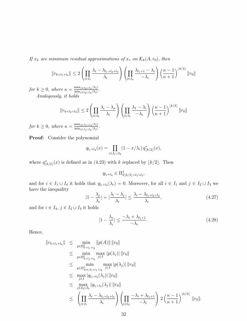
Proof: Consider the polynomial

qk+n−l(x) =n∏

i=l+1

(1− x/λi)q∗k(x),

30

where q∗k(x) is defined as in (4.23). Then qk+n−l ∈ Π1k+n−l, and for i ∈ l + 1, . . . , n it

holds that qk+n−l(λi) = 0. Moreover, for all i ∈ l+ 1, . . . , n and j ∈ 1, . . . , l we have theinequality

|1− λj/λi| = |λi − λj |/|λi| ≤ (λ1 − λi)/|λi|.Hence,

‖rk+n−l‖ ≤ minp∈Π1

k+n−l

‖p(A)‖ ‖r0‖

≤ maxj=1,...,n

|qk+n−l(λj)| ‖r0‖

= maxj=1,...,l

|qk+n−l(λj)| ‖r0‖

≤n∏

i=l+1

λ1 − λi|λi|

maxj=1,...,l

|q∗k(λj)| ‖r0‖.

The estimate is a simple consequence of the construction of qn+k−l. From the last expressionwe get immediately the assertion using (4.24) and (4.26). 2

This result is of interest, if, for one, there are only few negative eigenvalues, so that theestimate can be established after a small number of iterations, and if secondly the negativeeigenvalues are not too small, because otherwise the factor

∏(λ1 − λi)/|λi| will be large.

These situations do in general not occur in our applications. Nevertheless, we have in-cluded this result because it gives the idea how one might go about isolating some eigenvaluesin order to establish more refined convergence results than that in Theorem 4.3.8.

One situation we have found useful to look at is the case where there is one cluster oflarge eigenvalues and another cluster of eigenvalues of moderate size on the positive realline, and essentially the same distribution on the negative side of the origin. In this case thefollowing two results hold. They are generalizations of Theorem 4.3.10.

Theorem 4.3.11 Let A ∈ IRn×n be a nonsingular, symmetric indefinite matrix with eigen-values

λ1 ≥ . . . ≥ λl1 λl1+1 ≥ . . . ≥ λl1+l2 > 0,0 > λl1+l2+1 ≥ . . . ≥ λl1+l2+l3 λl1+l2+l3+1 ≥ . . . ≥ λn.

Let

I1 = 1, . . . , l1,I2 = l1 + 1, . . . , l1 + l2,I3 = l1 + l2 + 1, . . . , l1 + l2 + l3,I4 = l1 + l2 + l3 + 1, . . . , l1 + l2 + l3 + l4

= l1 + l2 + l3 + 1, . . . , n and

I = I1 ∪ I2 ∪ I3 ∪ I4.

31

If xk are minimum residual approximations of x∗ on Kk(A, r0), then

‖rk+l1+l4‖ ≤ 2

∏i∈I1

λi − λl1+l2+l3

λi

∏i∈I4

λl1+1 − λi−λi

(κ− 1

κ+ 1

)bk/2c‖r0‖

for k ≥ 0, where κ =maxj∈I2∪I3 |λj |minj∈I2∪I3 |λj|

.

Analogously, it holds

‖rk+l2+l3‖ ≤ 2

∏i∈I2

λi − λnλi

∏i∈I3

λ1 − λi−λi

(κ− 1

κ+ 1

)bk/2c‖r0‖

for k ≥ 0, where κ =maxj∈I1∪I4 |λj|minj∈I1∪I4 |λj |

.

Proof: Consider the polynomial

ql1+l4(x) =∏

i∈I1∪I4(1− x/λi) q∗bk/2c(x),

where q∗bk/2c(x) is defined as in (4.23) with k replaced by bk/2c. Then

ql1+l4 ∈ Π12bk/2c+l1+l4

,

and for i ∈ I1 ∪ I4 it holds that ql1+l4(λi) = 0. Moreover, for all i ∈ I1 and j ∈ I2 ∪ I3 wehave the inequality

|1− λjλi| = |λi − λj

λi| ≤ λi − λl1+l2+l3

λi, (4.27)

and for i ∈ I4, j ∈ I2 ∪ I3 it holds

|1− λjλi| ≤ −λi + λl1+1

−λi. (4.28)

Hence,

‖rk+l1+l4‖ ≤ minp∈Π1

k+l1+l4

‖p(A)‖ ‖r0‖

≤ minp∈Π1

k+l1+l4

maxj∈I|p(λj)| ‖r0‖

≤ minp∈Π1

2bk/2c+l1+l4

maxj∈I|p(λj)| ‖r0‖

≤ maxj∈I|ql1+l4(λj)| ‖r0‖

≤ maxj∈I2∪I3

|ql1+l4(λj)| ‖r0‖

≤∏i∈I1

λi − λl1+l2+l3

λi

∏i∈I4

−λi + λl1+1

−λi

2(κ− 1

κ+ 1

)bk/2c‖r0‖.

32

The estimate is a consequence of the construction of ql1+l4, following from (4.27), (4.28)and the estimates (4.24) and (4.26) for the Chebyshev approximation problem. The secondassertion can be shown by essentially the same arguments. 2

A special case of the situation analyzed in the previous theorem occurs in our applications.We encountered a distribution of eigenvalues where eigenvalues of moderate size were situatedin two clusters around the origin, and another cluster of large eigenvalues lay on the positiveside of the origin. This situation can be analyzed as a special case of the situation describedabove with l4 = 0.

Inclusion sets for the matrices we are interested in are often of the form

E = [−d,−ch2] ∪ [ch2, d]. (4.29)

Typically, h denotes a mesh parameter of increasingly small size. In this case

κ =d

ch2= O(h−2).

Rewriting the convergence governing factor in the form

κ− 1

κ+ 1= 1− 2

1

κ+ 1= 1− 2(

1

κ− 1

κ2 + κ) = 1− 2

1

κ+O(h4)

shows that convergence is determined by a factor

γ ≤ 1− 2h2c/d +O(h4)

for an inclusion set E of this form. It follows from the foregoing presentation (see (4.18 inparticular) that

‖rk‖‖r0‖

≤ minp∈Π1

k

maxi=1,...,n

|p(λi)| := γk. (4.30)

The factorγ = lim

k→∞γ

1/kk

is called the asymptotic convergence rate.If the eigenvalues of the indefinite matrix are not symmetric about the origin, but do

depend on a mesh size parameter, then the following result by Wathen, Fischer and Silvester[16] is of interest:

Theorem 4.3.12 Let A ∈ IRn×n be a nonsingular, symmetric indefinite matrix with eigen-values in the inclusion set

E = E(h) := [−a,−bh]∪ [ch2, d], a, b, c, d, h > 0. (4.31)

Then the asymptotic convergence rate γ can be estimated as follows:

γ ≤ 1− h3/2√bc/ad+O(h5/2).

33

This tells us that, although an asymmetric distribution of the eigenspectrum must ingeneral be judged disfavorably, we still profit from having a dependence of the spectrumbounds on a lower power of the small parameter h than in the symmetric case in (4.29).

4.3.2 Convergence Results for SYMMLQ

As we have seen in Section 4.2, if A is symmetric positive definite, one can use the functionvalue of F to measure convergence of the Galerkin approximation. This is a point common toboth SYMMLQ and the conjugate gradient method. However, since the conjugate gradientmethod can be applied only for positive definite matrices, whereas SYMMLQ works forindefinite matrices, too, where (4.4) has no solution, it is less clear how to measure progressin the indefinite case.

In the case of a positive definite system matrix, we can define the norm ‖.‖A by ‖x‖A =√xTAx and the corresponding scalar product 〈x, x〉A = xTAx. In Section 4.2 we have

derived the conjugate gradient method, and we have seen that the conjugate gradient methodminimizes the error ‖e‖A in every iteration, cf. (4.10). Since the conjugate gradient iteratesare the Galerkin approximations, we obtain for symmetric positive definite matrices A theestimate

‖ek‖A ≤ minp∈Π1

k

maxi=1,...,n

|p(λi)| ‖r0‖A,

corresponding to the result established for MINRES in (4.18). Since the estimates are exactlyof the same type, the convergence results derived above immediately carry over.

However, if A is indefinite, it defines no norm and corresponding scalar product, and thusthe initial estimate cannot be derived. Thus similar convergence results do not hold. Thisreflects the fact that the Galerkin approximation not necessarily exists in the indefinite case.

As for the minimum residual approximations, we still have finite convergence for theGalerkin approximations. This was already established in Theorem 4.3.5.

4.4 Implementation of SYMMLQ and MINRES

In Section 4.2 we have seen how the conjugate gradient method is derived and how thisapproach is motivated, namely by the minimization of the functional F given in (4.4). Thisapproach is no longer appropriate for the extension on the indefinite case. However, one canstill try to compute the approximation we relied on in the positive definite case in (4.9) oruse the approximation (4.12). In addition to this, another point of view motivates the choiceof Krylov subspaces.

Let X be an invariant subspace of A. X is an invariant subspace for A if and only ifAX = XB for some B ∈ IRm×m, where the m columns of X ∈ IRn×m span X . This meansthat the action of A on the m - dimensional subspace X is completely determined by B. Ifr0 ∈ X , then Ax = r0 can be solved in the following way: r0 = Xc holds for some c ∈ IRm,so solve By = c for y ∈ IRm, and the solution is x = Xy.

34

Thus the problem of dimension n × n is reduced to an m ×m system. This can resultin quite a computational advantage. So the plan is to find the smallest invariant subspacecontaining r0.

As we have seen in Section 4.2, the conjugate gradient method constructs a new searchdirection in every step of the iteration. The search directions p0, . . . , pj span the the Krylovsubspace of order j. Similarly, MINRES and SYMMLQ iterate on Krylov subspaces ofincreasing dimension. To proceed, we need to express the vectors in the Krylov subspace oforder j in terms of a basis for the subspace of order j + 1, i.e. to perform a change of basis.

We have the following transition from the basis for the j - dimensional subspace to thebasis of the j + 1 -dimensional:

AKj = [Ar0, A2r0, . . . , A

jr0]

= [r0, Ar0, A2r0, . . . , A

jr0]

0 . . . . . . 0

1. . .

...

0. . .

. . ....

.... . .

. . . 00 . . . 0 1

= Kj+1

0 . . . . . . 0

1. . .

...

0. . .

. . ....

.... . .

. . . 00 . . . 0 1

(4.32)

(4.33)

Here we simply employed the natural basis, given by the columns of Kj = [r0, . . . , Aj−1r0] forthe Krylov subspace Kj(A, r0) of order j. If we have orthogonal decompositions of the basismatrices Kj and Kj+1, i.e. Kj = QjRj , Kj+1 = Qj+1Rj+1, where Qj, Qj+1 are orthogonaland Rj, Rj+1 upper triangular, we see the following.

AQjRj = Qj+1Rj+1

(0T

Ik

)

AQj = Qj+1Rj+1

(0T

Ik

)R−1j

= Qj+1Hj+1, (4.34)

where Hk+1 can be shown to be upper Hessenberg. A matrix H ∈ IRn×m is called an upperHessenberg matrix if hij = 0 for all (i, j) with i > j+1. This means that H is upper diagonalwith possibly additional entries in the lower subdiagonal.

The previous presentation in (4.34) indicates the implementation of another basis ofthe Krylov subspace Ki(A, r0) of order i than the natural basis. In fact these vectors are

35

computationally near to linear dependence. Additionally, orthogonal bases often are of greatcomputational advantage. Their usage will be introduced in Section 4.4.1.

Upper Hessenberg matrices play an important role in the successive construction of aninvariant subspace. This becomes obvious in the following theorem.

Theorem 4.4.1 Let A ∈ IRn×n be symmetric and let v1, . . . , vm+1 be linearly independentsuch that

spanv1, . . . , vi = Ki(A, r0), i = 1, . . . ,m+ 1.

There exists an upper Hessenberg matrix Tm ∈ IR(m+1)×m such that

AVm = Vm+1Tm, (4.35)

where Vm+1 denotes the matrix with columns v1, . . . , vm+1. The upper Hessenberg matrix Tmis uniquely determined by A and v1, . . . , vm+1. If Vm+1 is orthonormal, then

V ∗mAVm = Tm, (4.36)

where Tm ∈ IRm×m is the matrix obtained from Tm by deleting the last row. In particular,Tm and Tm are tridiagonal.

Proof: Since spanv1, . . . , vi = Ki(A, r0), we obtain Avi ∈ Ki+1(A, r0). Moreover, sincev1, . . . , vi+1 is a basis of Ki+1(A, r0) there exist scalars tij, j = 1, . . . , i+ 1, such that

Avj =i+1∑j=1

tijvj.

The scalars tij, j = 1, . . . , i + 1, are uniquely determined by Avi and v1, . . . , vi+1. Setting

tij = 0, if i > j + 1,

and defining Tm to be the matrix with entries tij we obtain (4.35). We can see from theconstruction that Tm is an upper Hessenberg matrix. The equation (4.36) is an immediateresult of (4.35) and the orthogonality of Vm+1. If A is symmetric, then V ∗mAVm is symmetric.Therefore, the upper Hessenberg matrix Tm in (4.36) has to be symmetric. This impliesthat Tm has to be a tridiagonal matrix. 2

Theorem 4.4.2 Let A ∈ IRn×n and let v ∈ IRn.

1. Ki(QAQ∗, Qv) = QKi(A, v) for unitary Q.

2. Let vectors v1, . . . , vm be given such that

spanv1, . . . , vi = Ki(A, v1) ∀i = 1, . . . ,m,

thenspanv1, . . . , vi, Avi = Ki+1(A, v1) ∀i = 1, . . . ,m.

36

Proof:

1. This follows by the orthogonality of Q.

2. Sincespanv1, . . . , vi = spanv1, Av1, . . . , A

i−1v1,we find that

spanv1, . . . , vi, Avi ⊂ Ki+1(A, v)

On the other hand we have that

Ki+1(A, v1) = Ki(A, v1) ∪ (Aiv1)

and Ki(A, v1) = spanv1, . . . , vi. Moreover,

Aiv1 = AAi−1v1 ∈ AKi(A, v1) = spanAv1, . . . , Avi,

and, since spanv1, . . . , vi−1 = Ki−1(A, v1),

spanAv1, . . . , Avi−1 = AKi−1(A, vi) = span(Av1, . . . AAi−2v1

⊂ Ki(A, v1) = spanv1, . . . , vi.

Hence Ki−1(A, v1) ⊂ spanv − 1, . . . , vi, Avi.

2

Part 2 of the preceding theorem is important for the numerical computation of a solu-tion for the linear system Ax = r0. MINRES and SYMMLQ successively construct a basisv1, . . . , vi of Ki(A, r0). Instead of effectively computing powers Ai and then taking thematrix vector product Air0, a basis for Ki+1(A, r0) can then be computed for the expense ofone matrix - vector multiplication, namely Avi, because Ki+1(A, v1) = v1, . . . , vi, Avi. InPart 1 we see how a unitary transformation of A can be expressed in terms of the Krylovsubspace generated by A.

We now turn to the issue of computing orthogonal bases for the subspace underlying theiterative process.

4.4.1 Orthogonal Bases for the Krylov Subspaces

Using spanr0, . . . , Am−1r0 as a representation for Km(A, r0), the Gram–Schmidt algorithmsuccessively orthogonalizes the vectors Ajr0 against the previously obtained orthogonal vec-tors vi, i = 1, . . . , j. This is not done by computing Ajr0. Instead of using Ajr0 as the newcolumn and orthogonalizing it against the orthonormal vectors v1, . . . , vj already obtained,Avj is used for this process. This gives Kj+1 = (Kj , Avj).

37

Since the classical Gram–Schmidt is numerically unstable (see e.g. [8], p.218), one oftentakes refuge to the modified Gram–Schmidt process, which is in this context known as theArnoldi process.

Algorithm 4.4.3 (Arnoldi Process)

1. given r0 and m

2. set v1 = r0/‖r0‖

3. for j = 1, . . . ,m− 1

3.1. vj+1 = Avj

3.2. for i = 1, . . . , j

3.2.1. tij = 〈vj+1, vi〉3.2.2. vj+1 = vj+1 − tijvi

3.3. tj+1,j = ‖vj+1‖3.4. if tj+1,j = 0 stop

3.5. vj+1 = vj+1/tj+1,j

The Arnoldi process computes the entries tij, j = 1, . . . , i+ 1, of a matrix that representsthe change of basis as given in (4.32). If A is symmetric, and v1, . . . , vm are the vectorsgenerated by Algorithm (4.4.3), then we obtain from Theorem 4.4.1 that

V ∗mAVm = Tm

for a symmetric tridiagonal matrix Tm ∈ IRm×m. In particular we have that tij = 0 fori < j − 1. Therefore the j - th step of Algorithm (4.4.3) reduces to

vj+1 = Avj − 〈Avj, vj−1〉vj−1 − 〈Avj, vj〉vj (4.37)

vj+1 = vj+1/‖vj+1‖, (4.38)

where we formally set v0 = 0. This simplification shows that the new vector only has to beorthogonalized against the preceding two orthogonal basis vectors.

With δj = ‖vj‖, the orthogonality of vi, i = 1, . . . , j, and the symmetry of A we obtain

〈Avj, vj−1〉 = 〈vj, Avj−1〉= 〈vj, Avj−1 − 〈Avj−1, vj−2〉vj−2 − 〈Avj−1, vj−1〉vj−1〉= 〈vj, vj〉 = 1

δj‖vj‖2 = δj.

Furthermore,〈Avj, vj〉 = 〈Avj − δjvj−1, vj〉.

Using this representation, we obtain the so–called Lanczos Tridiagonalization:

38

Algorithm 4.4.4 (Lanczos Tridiagonalization)

1. given r0 and m

2. set v1 = r0, v0 = 0 and δ1 = ‖v1‖

3. for j = 1, . . . ,m− 1

3.1. if δj = 0 stop

3.2. vj = vj/δj

3.3. vj+1 = Avj − δjvj−1

3.4. γj = 〈vj+1, vj〉3.5. vj+1 = vj+1 − γjvj3.6. δj+1 = ‖vj+1‖

Note that the process stops if δj+1 = 0. This means that the potential new basis vectorAvj = vj+1 is linearly dependent of the preceding basis vectors. It lies entirely in the directionof the preceding basis vectors, and so the orthogonalization process only leaves over the zerovector. In our context this means that an invariant subspace is encountered.

From Algorithm 4.4.4 one can see that the vectors v1, . . . , vj+1 satisfy

V ∗j AVj = Tj, (4.39)

AVj = Vj+1Tj = VjTj + δj+1vj+1eTj , (4.40)

where Vj = [v1, . . . , vj], Vj+1 = [v1, . . . , vj+1] and Tj, Tj are tridiagonal matrices as given inTheorem 4.4.1.

The matrix Tj ∈ IRj×j is of the following form for all j = 1, . . . ,m:

Tj = tridiag(δj, γj, δj+1) =

γ1 δ2

δ2 γ2 δ3

. . .. . .

. . .

δj−1 γj−1 δjδj γj

, (4.41)

and Tj is obtained by deleting the last row of Tj ∈ IR(j+1)×j, where

Tj = tridiag(δj, γj, δj+1) =

γ1 δ2

δ2 γ2 δ3

. . .. . .

. . .

δj−1 γj−1 δjδj γj

δj+1

. (4.42)

39

With the help of these matrices we now derive an alternative formulation for the problemswe try to solve, i.e. for the approximations to the exact solution we seek.

Since spanv1 = spanr0 = K1(A, r0) we have

βv1 = βVme1 = r0, (4.43)

with β = ‖r0‖ ∈ IR. If v1, . . . , vj are orthonormal for j = 1, . . . ,m, then Theorem 4.4.1 and(4.43) yield that

0 = 〈Axj − r0, v〉 ∀v ∈ Kj(A, r0)= 〈AVjyj − r0, Vjy〉 ∀y ∈ IRj

= 〈AVjyj − Vjβe1, Vjy〉 ∀y ∈ IRj.

This holds if and only if

0 = 〈V ∗j AVjyj − βe1, y〉 ∀y ∈ IRj

= 〈Tjyj − βe1, y〉 ∀y ∈ IRj.

Thus the problem (4.11) is equivalent to solving

Tjy = βe1 = ‖r0‖e1. (4.44)

Similarly, the problem formulation (4.12) for MINRES can be written as

miny∈IRj

1

2‖AVjy − r0‖2 = min

y∈IRj1

2‖Vj+1Tjy − r0‖2. (4.45)

Since r0 = βVj+1e1 and, if v1, . . . , vj for all j = 1, . . . ,m are orthonormal, ‖Vj+1y‖ = ‖y‖ forall y ∈ IRj+1, this leads to the following problem equivalent to (4.12):

miny∈IRj

1

2‖Tjy − βe1‖2, (4.46)

where β = ‖r0‖.

In Section 4.2 we have seen that a solution zj to (4.44) may not exist if A is not positivedefinite. The least squares problem (4.46), however, is always uniquely solvable.

Theorem 4.4.5 Suppose that A is nonsingular and that δ2, . . . , δj are nonzero. If δj+1 6= 0,then

miny∈IRj‖Tjy − βe1‖2 (4.47)

has a unique solution yj ∈ IRj. If δj+1 = 0, then x = Vjyj solves Ax = r0, where yj solves(4.44) and, as a consequence, solves (4.47) with zero residual.

40

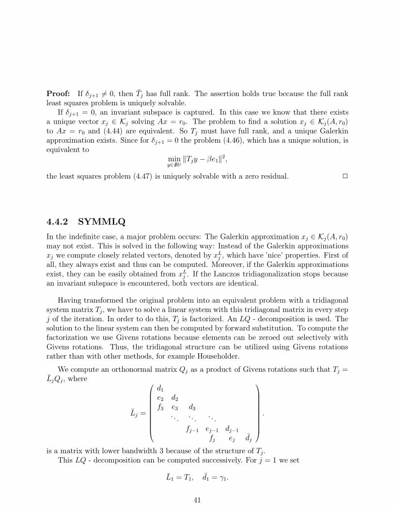
Proof: If δj+1 6= 0, then Tj has full rank. The assertion holds true because the full rankleast squares problem is uniquely solvable.

If δj+1 = 0, an invariant subspace is captured. In this case we know that there existsa unique vector xj ∈ Kj solving Ax = r0. The problem to find a solution xj ∈ Kj(A, r0)to Ax = r0 and (4.44) are equivalent. So Tj must have full rank, and a unique Galerkinapproximation exists. Since for δj+1 = 0 the problem (4.46), which has a unique solution, isequivalent to

miny∈IRj‖Tjy − βe1‖2,

the least squares problem (4.47) is uniquely solvable with a zero residual. 2

4.4.2 SYMMLQ

In the indefinite case, a major problem occurs: The Galerkin approximation xj ∈ Kj(A, r0)may not exist. This is solved in the following way: Instead of the Galerkin approximationsxj we compute closely related vectors, denoted by xLj , which have ’nice’ properties. First ofall, they always exist and thus can be computed. Moreover, if the Galerkin approximationsexist, they can be easily obtained from xLj . If the Lanczos tridiagonalization stops becausean invariant subspace is encountered, both vectors are identical.

Having transformed the original problem into an equivalent problem with a tridiagonalsystem matrix Tj, we have to solve a linear system with this tridiagonal matrix in every stepj of the iteration. In order to do this, Tj is factorized. An LQ - decomposition is used. Thesolution to the linear system can then be computed by forward substitution. To compute thefactorization we use Givens rotations because elements can be zeroed out selectively withGivens rotations. Thus, the tridiagonal structure can be utilized using Givens rotationsrather than with other methods, for example Householder.

We compute an orthonormal matrix Qj as a product of Givens rotations such that Tj =LjQj, where

Lj =

d1

e2 d2

f3 e3 d3

. . .. . .

. . .

fj−1 ej−1 dj−1

fj ej dj

.

is a matrix with lower bandwidth 3 because of the structure of Tj.This LQ - decomposition can be computed successively. For j = 1 we set

L1 = T1, d1 = γ1.

41

Assume that Givens rotations G2j, . . . , Gjj have been computed such that Tj is transformedinto the special lower triangular form

TjG2j · · ·Gjj = Lj.

Here the jth Givens rotation is

Gj =

11

. . .

1cj sjsj −cj

∈ IRj×j ,

and Gij , i ≤ j, denote

Gij =

(Gi 00 Ij−i

)∈ IRj×j,

so that Gjj = Gj . Then

Tj+1G2,j+1 . . . Gj,j+1 =

d1 0e2 d2 0f3 e3 d3 0

. . .. . .

. . . 0fj−1 ej−1 dj−1 0

fj ej dj δj+1

fj+1 ej+1 γj+1,

.

wherefj+1 = sjδj+1, ej+1 = −cjδj+1.

The application of the Givens rotation Gj+1

Gj+1 =

11

. . .

1cj+1 sj+1

sj+1 −cj+1

∈ IRj+1×j+1.

withdj =

√d2j + δ2

j+1, cj+1 = dj/dj , sj+1 = δj+1/dj (4.48)

42

(Gj+1 is designed to zero out the superdiagonal entry δj+1) to Tj+1G2,j+1, . . . , Gj,j+1 yields

Tj+1G2,j+1 · · ·Gj,j+1Gj+1,j+1 = Lj+1 =

d1

e2 d2

f3 e3 d3

. . .. . .

. . .

fj−1 ej−1 dj−1

fj ej djfj+1 ej+1 dj+1

.

with dj+1 = sj+1ej+1 − cj+1γj+1 and ej+1 = cj+1ej+1 + sj+1γj+1.

If δj+1 6= 0, then dj =√d2j + δ2

j+1 > 0. Clearly Lj+1 is singular if dj+1 = 0. If dj+1 6= 0and the Arnoldi process has not yet stopped with δj+1 = 0, then di > 0, i = 1, . . . , j, so thatLj+1 is nonsingular. Hence, Lj+1 is singular if and only if dj+1 = 0.

Additionally defineQj = GT

jj · · ·GT2j,

w1 = v1,Wj = (w1, . . . , wj−1, wj) = VjQ

Tj ,

zj = (ζ1, . . . , ζj−1, ζj) = Qjyj.

Since the Givens rotations Gj only transforms columns j and j − 1, we have that

Wj = VjQTj

= (w1, . . . , wj−1, wj)= (Vj−1|vj)G2,j . . . Gj−1,jGjj

= (Vj−1G2,j . . .Gj−1,j |vj)Gjj

= (Vj−1QTj−1|vj)Gjj

= (Wj−1|vj)Gjj

= (w1, . . . , wj−1, vj)Gjj .

Using the definition of Gjj we find that the columns j and j − 1 of Wj can be obtainedfrom

wj−1 = cjwj−1 + sjvj, wj = sjwj−1 − cjvj. (4.49)

With these definitions, the alternative formulation (4.44) for the SYMMLQ problem canbe written as

Tjyj = LjQjyj = Lj zj = ‖r0‖e1, (4.50)

and the Galerkin approximation for the solution of Ax = r0 is given by

xj = Vjyj = VjQTj Qjyj = Wj zj.

The vector zj is computed as the solution of (4.50). The transition to Wj amounts to anotherchange of basis. We derived the formulation (4.44) for the original problem in changing from

43

the ’natural’ basis r0, Ar0, . . . , Aj−1r0 to an orthonormal basis v1, . . . , vj of Kj(A, r0).Now we consider as the underlying basis the columns of Wj = VjQT

j . Storage of the full matrixWj can be prohibitive for large dimensional problems. Fortunately, it is not necessary tostore all previous basis vectors and explicitly form Wj zj. This will become obvious when arecursion for the iterates is derived.

The iterates xj = Wj zj are the Galerkin approximations for the solution of Ax = r0.Since we are interested in a solution of Ax = b and since r0 = b− Ax0, the approximationfor the solution x∗ is given by x0 + xj = Wj zj. The iterates x0 + xj will be denoted by xj,i.e. xj = x0 + Wjzj.

We have seen that the matrix Lj is singular if and only if dj = 0. In this case the Galerkinapproximation may not exist, and it is certainly not unique. To overcome this problem, wechange to slightly different iterates as we already indicated. In addition to Lj we defineLj ∈ IRj×j to be the matrix obtained from Lj by replacing dj with dj . The matrix Lj is theupper j × j - submatrix of Lj+1. Moreover, we set

Wj = (w1, . . . , wj−1, wj)

(Wj is obtained from Wj+1 by deleting the last column), and

zj = (ζ1, . . . , ζj−1, ζj),

where zj solvesLjzj = ‖r0‖ e1.

Wj is obtained from Wj+1 by deleting the last column. As it is suggested by the notation,the solution zj of Ljzj = ‖r0‖e1 effectively differs from the solution zj of Ljz = ‖r0‖e1 onlyin one component. The first j − 1 components of zj and zj are identical, and for the j-thcomponent we obtain that ζj = cj+1 ζj. This follows from the relation (4.48) between dj anddj .

SettingxLj = x0 +Wjzj,

the vectors xLj obey the recursion

xL0 = x0, xLj = x0 +Wj−1zj−1 + ζjwj = xLj−1 + ζjwj, j ≥ 1.

This recursion shows that it is not necessary to store all the vectors wj. Instead, the currentiterate is obtained as a linear combination of the previous vector xLj−1 and the latest basisvector. The vectors vj, wj can be formed, used and discarded one by one.

For the Galerkin approximation xj we have

xj = x0 + Wj zj = x0 +Wj−1zj−1 + ζjwj = xLj−1 + ζjwj.

This can be written asxj = xLj + ζj(wj/cj+1 − wj)

44

if we use the recursion for xLj and the relation ζj = cj+1ζj . The recursion (4.49) for wj, wjyields

cj+1wj = c2j+1wj + cj+1sj+1vj+1 = c2

j+1wj − sj+1(wj+1 − sj+1wj) = wj − sj+1wj+1

and thus we have the transition formula

xj = xLj + (ζjsj+1/cj+1)wj+1. (4.51)

Thus, one can use the recursion for xLj throughout the iteration and in the final step onecan use this formula to compute xj from xLj .

The iteration is terminated if the residual is small. The residual can be monitored duringthe iteration without knowing the current Galerkin approximation xj because the followingformula for the residual holds:

Axj − b = AVjyj − r0 = Vj(Tjyj − ‖r0‖e1) + δj+1vj+1eTj yj = δj+1vj+1y

(j)j ,

where the vector yj is the solution of (4.44) and y(j)j denotes the j-th component of yj. The

vector yj is not directly available, but its last component can be computed cheaply. FromTj = T Tj = QT

j LTj we obtain that

LTj yj = ‖r0‖Qje1.

Since Qj = GTjj · · ·GT

2j , the last row of the equation is given by

djy(j)j = ‖r0‖s2 · · · sj .

thus−rj = Axj − r0

= δj+1vj+1‖r0‖s2 · · · sj/dj= vj+1‖r0‖s2 · · · sj sj+1/cj+1,

(4.52)

and so‖rj‖ = ‖r0‖ |s2 . . . sj sj+1/cj+1| = ‖rj−1‖ |sj+1cj/cj+1|. (4.53)

If δj0 = 0 for some j0, then the Krylov space is invariant, i.e. Kj(A, r0) = Kj0−1(A, r0) forall j ≥ j0 − 1, and the solution is found. We are then in the situation AVm = VmTm. Thisis also shown by the formula for the residual: If δj0 = 0, then rj0−1 = 0, and xj0−1 solves thesystem.

The formulas (4.51), (4.52) and (4.53) are valid if and only if the Galerkin approximationsexist, i.e. if dj 6= 0. Because of the relation (4.48) this is equivalent to cj+1 6= 0.

Although the Galerkin approximation may not exist, the approximations xLj always exist.Therefore we compute these instead of the vectors xj throughout the iteration and use (4.51)to compute the Galerkin approximation at the end. To show that the method introducedabove is well–defined we need to show that Lj is nonsingular.

45

Lemma 4.4.6 Let A ∈ IRn×n be nonsingular, and let j0 be such that δj0+1 = 0, δ1, . . . δj0 6=0. Then Lj is nonsingular for j = 1, . . . , j0.

Proof: Let j ≤ j0 be the first index such that Lj is singular. Then d1, . . . dj−1 6= 0, anddj = 0. This means that dj = δj+1 = 0. With (4.39) this yields

AVj = VjTj.

Thus, since A is nonsingular and Vj is orthogonal, Tj is nonsingular. If δj+1 = 0, thenLj = Lj = TjQ

Tj . This shows that Lj cannot be singular. 2

If δj0 = 0, then the exact solution of Ax = b is found. In this case Lj0 = Lj0 and xj0 = xLj0.In theory, the iteration stops with δj+1 = 0, and then the iterates that are actually computed,the Galerkin approximation and the exact solution coincide. However, the stopping criterionin practice is a small residual.

The foregoing presentation leads to the following implementation of the algorithm.

Algorithm 4.4.7 (SYMMLQ)

1. given A ∈ IRn×n symmetric, b ∈ IRn, x0 ∈ IRn

2. compute r0 = b− Ax0, set

2.1. v1 = r0

2.2. δ1 = ‖r0‖

3. if δ1 6= 0, then v1 = v1/δ1;

4. else v1 = v1 = 0;

5. endif

6. w1 = v1, v0 = 0, xL0 = x0

7. while ‖rj‖ ≥ ε

7.1. vj+1 = Avj − δjvj−1

7.2. γj = 〈vj+1, vj〉7.3. vj+1 = vj+1 − γjvj7.4. δj+1 = ‖vj+1‖7.5. if δj+1 6= 0, then vj+1 = vj+1/δj+1

7.6. else vj+1 = vj+1 = 0;

46

7.7. endif

7.8. if j = 1, then

7.8.1. dj = γj

7.8.2. ej+1 = δj+1

7.9. elseif j > 1, then

7.9.1. Apply Givens rotation Gj to row j:

7.9.2. dj = sj ej − cjγj7.9.3. ej = cj ej + sjγj

7.9.4. Apply Givens rotation Gj to row j + 1:

7.9.5. fj+1 = sjδj+1

7.9.6. ej+1 = −cjδj+1

7.10. endif

7.11. determine Givens rotation Gj+1

7.11.1. dj =√d2j + δ2

j+1

7.11.2. cj+1 = dj/dj

7.11.3. sj+1 = δj+1/dj

7.12. if j = 1, then ζ1 = δ1/d1;

7.13. elseif j = 2 then ζ2 = −ζ1e2/d2;

7.14. elseif j > 2, then ζj = (−ζj−1ej − ζj−2fj)/dj ;

7.15. endif

7.16. wj = cj+1wj + sj+1vj+1

7.17. wj+1 = sj+1wj − cj+1vj+1

7.18. xLj = xLj−1 + ζjwj

7.19. if j = 1, then res = ‖r0‖ · |s2|;7.20. if j > 1, then res = res ·|sj+1|;7.21. endif

7.22. if cj+1 6= 0, then ‖rj‖ = res/cj+1

7.23. else set ‖rj‖ =∞7.24. endif

end

8. xj = xLj + (ζjsj+1/cj+1)wj+1

47

Remark: The equality ‖rj‖ = ∞ holds if and only if cj+1 = 0. From (4.48) one can seethat cj+1 = 0 if and only if dj = 0, i.e. if and only if Lj is rank deficient. Moreover, from(4.51) one can see that a Galerkin approximation does not exist if cj+1 = 0.

In summary: The equality ‖rj‖ = ∞ corresponds to the nonexistence of the Galerkinapproximation.

4.4.3 MINRES

Let v1, . . . , vj be the orthonormal vectors generated by the Lanczos tridiagonalization process.MINRES solves in every step

minx∈Kj(A,r0)

‖Ax− r0‖. (4.54)

Considering the formulation (4.46) we see that this least squares problem is equivalent tosolving

V ∗j A2Vjy = V ∗j Ar0

for y ∈ Kj(A, r0), where Vj = [v1, . . . , vj]. If yj is the solution, the iterate is xj = Vjyj. Usingthe formulation given in (4.39), which led to (4.46), we find that

V ∗j A2Vj = TjV ∗j+1Vj+1Tj

= T 2j + δ2

j+1ejeTj ,

V ∗j Ar0 = ‖r0‖V ∗j Av1 = ‖r0‖Tje1.

Hence we have to solve(T 2

j + δ2j+1eje

Tj )y = ‖r0‖Tje1. (4.55)

We used an LQ decomposition of Tj to derive the implementation of SYMMLQ. We usea similar approach for MINRES. Let Lj, Lj and Qj denote the matrices introduced in theprevious section.

Additionally define

Lj =

d1

e2 d2

f3 e3 d3

. . .. . .

. . .

fj−1 ej−1 dj−1

fj ej dj δj+1

,

then

LjGj+1 =

d1

e2 d2

f3 e3 d3

. . .. . .

. . .

fj−1 ej−1 dj−1

fj ej dj 0

48

by construction of the (j + 1)st Givens rotation. The first j columns of LjGj+1 are equal tothe matrix Lj obtained from Lj by replacing dj with dj . Hence,

T 2j + δ2

j+1ejeTj = LjL

Tj + δ2

j+1ejeTj = LjL

Tj = LjGj+1G

Tj+1L

Tj = LjL

Tj .

Using this, we can rewrite the alternative formulation (4.55) as

LjLTj y = ‖r0‖LjQje1. (4.56)

By construction of Lj , Lj and the relation cj+1 = dj/dj (cf. (4.48)) we find that

Lj = LjDj , Dj = diag(1, . . . 1, cj+1). (4.57)

Since Lj is nonsingular we obtain the following linear equation which is equivalent to (4.56)

LTj y = ‖r0‖DjQje1 (4.58)

The definition of Qj = GTjj . . .G

T2j and the structure of the Givens rotations yield that the

components of‖r0‖DjQje1 = tj = (τ1, . . . , τj)

T

obeyτ1 = ‖r0‖c2, τi = ‖r0‖s2s3 . . . sici+1, i = 2, . . . j. (4.59)

Since LTj is an upper triangular matrix, the solution yi of (4.58) has to be computed bysolving the system backwards. Hence yj can only be computed if LTj is completely known.Since yj is computed by backward substitution, there is no obvious connection between yjand yj+1, j−1, . . . ,m−1. To obtain a recursion for the minimum residual iterates, we define

Mj = (m1, . . . ,mj) = VjL−T . (4.60)

Then the solution of (4.54) is given by

xMj = Vjyj = VjL−Tj LTj yj = Mjtj = xMj−1 +mjτj .

From (4.60) and from the definition of Lj we obtain that the columns of Mj satisfy

mj−2fj +mj−1ej +mjdj = vj,

ormj = (vj −mj−2fj −mj−1ej)/dj .

As in the previous cases, the minimum residual iterates recursively defined by (4.54) areapproximations of the solution of Ax = r0. Since we are interested in a solution of Ax = band since r0 = b − Ax0, the approximation of the solution x∗ = A−1b is given as x0 + xMj .Therefore we use a recursion for x0 +xMj . We find that (denoting x0 +xMj by xMj ) xMj obeys

xM0 = x0, xMj = xMj−1 +mjτj ,

49

where x0 is the given initial approximation. The corresponding residual can be written as

rj = b− AxMj = r0 − AVjyj = Vj‖r0‖e1 − VjTjyj − vj+1δj+1eTj yj, (4.61)

where yj is the solution of (4.58). Using (4.59) and the definition of yj we find that the lastcomponent of yj is given by

eTj yj = y(j)j = ‖r0‖s2s3 · · · sjcj+1/dj .

Since sj = δj+1/dj , this implies that

δj+1eTj yj = ‖r0‖s2s3 . . . sjsj+1cj+1. (4.62)

With T Tj = Tj = QTj L

Tj , (4.57) and (4.58) we obtain the equation

‖r0‖e1 − Tjyj = QTj (‖r0‖Qje1 −DjLTj yj)

= QTj (‖r0‖Qje1 − ‖r0‖D2

jQje1)= QT

j (‖r0‖(I −D2j )Qje1).

Due to the structure of Dj , (4.57) and the structure of the Givens rotations we obtain thatQje1 = s2s3 . . . sj and

‖r0‖e1 − Tjyj = QTj (‖r0‖(I −D2

j )Qje1)= ‖r0‖s2s3 . . . sj(1− c2

j+1)QTj ej

= ‖r0‖s2s3 . . . sjs2j+1.

(4.63)

Combining (4.61), (4.62), (4.63) and the fact that the vectors vi are othonormal we candeduce that

‖rj‖2 = ‖r0‖2(s2s3 · · · sj)2s4j+1 + ‖r0‖2(s2s3 · · · sj)2s2

j+1c2j+1 = ‖r0‖2(s2s3 · · · sj)2s2

j+1

This gives as formula for the residual norm :

‖rj‖ = ‖r0‖ |s2s3 · · · sjsj+1| = ‖rj−1‖ |sj+1|.

The above presentation leads to the final form of the MINRES algorithm.

Algorithm 4.4.8 (MINRES)

1. given A ∈ IRn×n symmetric, b ∈ IRn, x0 ∈ IRn.

2. compute r0 = b− Ax0, set

2.1. v1 = r0

2.2. δ1 = ‖r0‖

50

2.3. v0 = 0,m0 = m−1 = 0

3. while ‖rj‖ > ε

3.1. if δj 6= 0, then vj = vj/δj;

3.2. else vj = vj = 0;

3.3. endif

3.4. vj+1 = Avj − δjvj−1

3.5. γj = 〈vj+1, vj〉,3.6. vj+1 = vj+1 − γjvj3.7. δj+1 = ‖vj+1‖3.8. if j = 1, then

3.8.1. dj = γj3.8.2. ej+1 = δj+1

3.9. elseif j > 1, then

3.9.1. Apply Givens rotation Gj to row j:

3.9.2. dj = sj ej − cjγj3.9.3. ej = cj ej + sjγj3.9.4. Apply Givens rotation Gj to row j + 1:

3.9.5. fj+1 = sjδj+1

3.9.6. ej+1 = −cjδj+1

3.10. endif

3.11. Determine Givens rotation Gj+1

3.11.1. dj =√d2j + δ2

j+1,

3.11.2. cj+1 = dj/dj3.11.3. sj+1 = δj+1/dj

3.12. if j = 1, then τ1 = ‖r0‖c2

3.13. elseif j > 1, then τj = ‖r0‖s2s3 . . . sj cj+1/cj

3.14. endif

3.15. mj = (vj −mj−1ej −mj−2fj)/dj

3.16. xj = xj−1 + τjmj

3.17. ‖rj‖ = |sj+1| ‖rj−1‖

end

51

Chapter 5

Preconditioning

5.1 The Issue of Preconditioning

We have seen that the convergence of MINRES and SYMMLQ is mainly determined bythe distribution of the eigenvalues of the system matrix. Roughly one can say that theconvergence is better when the eigenvalues are clustered. More detailed results have beendiscussed in Section 4.3. This is the reason why we try to precondition the matrices underconsideration.

The general aim of preconditioning for a symmetric matrix A is to find a nonsingularmatrix P such that

P−1AP−T

has a better distribution of eigenvalues than the original system matrix A. One often triesto find P such that the condition number of the preconditioned matrix is much smaller thanthe condition number of A. This corresponds to a shrinkage of the spectrum. Often, theouter bounds of the eigenspectrum of a matrix arising from a finite element discretizationare bounded by a constant, while the inner bounds depend on the mesh constant and movetowards the origin with increasing fineness of the mesh. In this case one tries to move smalleigenvalues away from zero while leaving large eigenvalues essentially unchanged. But thisis not the only issue. By preconditioning, the distribution of the eigenvalues in the spectrumcan be favorably altered, not only the size of the spectrum. Moreover, preconditioning is onlyuseful if the gain due to better distribution of the eigenvalues and smaller condition numberis not destroyed by computational expensive matrix operations. Therefore the solution oflinear systems Py = z should be cheap.

Instead of Ax = b we consider the preconditioned system

Ax = b,

withA = P−1AP−T , x = P Tx, b = P−1b,

where P ∈ IRn×n is a nonsingular matrix.

52

For a nonsingular and symmetric matrix A ∈ IRn×n, the spectral condition number,denoted by κ2(A), is given by

κ2(A) =λ

λ,

where λ denotes the eigenvalue of A with largest absolute value, and λ the eigenvalue smallestin absolute value.

A point that is important about the 2–norm condition number – which is the conditionnumber we constantly consider – for the construction of preconditioners is the fact that theeigenvalues of P−1AP−T , A(PP T )−1 and of (PP T )−1A are identical. Thus it is sufficient toconsider (PP T )−1A or A(PP T )−1 instead of P−1AP−T . For the construction of precondition-ers for symmetric systems we have to find a symmetric positive definite matrix M palyingthe role of PP T such that M is a good and computationally cheap approximation for A−1.Since M is symmetric positive definite, there exists a Cholesky decomposition M = PP T ,and the preconditioner can be chosen from this decomposition. However, in many cases thisdecomposition is only used formally. The expenses are often judged to high. In the analysisit is sufficient to consider (PP T )−1A = M−1A. Why this is sufficient will be shown in thisfollowing Section 5.2.

5.2 The Preconditioned Algorithms

First we turn to the changes introduced in the implementation of the iterative solvers by pre-conditioning. Of course, it would be possible to simply apply the methods to the transformedsystem and proceed as before. But then we have to pay a lot of unnecessary expenses. Firstof all, applying MINRES and SYMMLQ to the transformed system means that P−1 and itstranspose can be computed and can, hopefully, be effectively applied. This is not alwaysthe case. Often enough, a preconditioner M is known, and a decomposition M = PP T isknown to exist, but one does not want to pay the expenses of effectively computing thisdecomposition. Secondly, this approach requires one matrix vector product A · x in eachiteration, which means in effect solving a linear system with P and P T in each iterationand applying A. At the end of the process, the solution provided by the iteration has to betransformed to a solution of the unpreconditioned system. These expenses can be reducedby the changes we present in this section.

If we apply the MINRES and SYMMLQ to the transformed system

Ax = b, (5.1)

then we iterate on Krylov subspaces Kj(P−1AP−T , P−1r0).

In each step j, MINRES minimizes

‖Ax− r0‖22 = ‖P−1AP−TP Tx− P−1r0‖2

2

= ‖P−1(AP−TP Tx− r0)‖22

53

= ‖P−1(Ax− r0)‖22

= 〈P−TP−1(Ax− r0), Ax− r0〉= ‖Ax− r0‖2

M−1. (5.2)

SYMMLQ computes iterates xj such that

〈Axj − r0, v〉 = 0 ∀v ∈ Kj(P−1AP−T , P−1r0). (5.3)

This is equivalent to searching for vectors xj such that

〈P−1AP−TP Txj − P−1r0, v〉 = 〈P−1(Axj − r0), v〉 = 0 ∀v ∈ Kj(P−1AP−T , P−1r0).

If we apply Algorithm 4.4.7 to the equation

Ax = b, (5.4)

withA = P−1AP−T , x = P Tx, b = P−1b,

then we basically have to replace the matrix A in the algorithm by

A = P−1AP−T ,

the vectors vj, vj by

vj = P Tvj,˜vj = P T vj,

and the residual rj by the transformed residual

rj = P−1rj.

The Lanczos process for the transformed problem Ax = b takes the vectorsP−1r0, (P−1AP−T )P−1r0, . . . , (P−1AP−T )j−1P−1r0, or, equivalently, the vectors P−1r0,P−1AM−1r0, . . . , P−1(AM−1)j−1r0, and orthogonalizes them against previously computedbasis vectors v1, . . . , vj, where v1 = P−1r0/‖P−1r0‖. The result is an orthogonal basisv1, . . . , vj for the underlying Krylov spaces Kj(P−1AP−T , P−1r0), j = 1, . . . ,m. The processis given as follows.

Algorithm 5.2.1 (Lanczos Tridiagonalization, Version 1)

1. given r0 and m

2. set ˜v1 = r0, v0 = 0 and δ1 = ‖˜v1‖

54

3. for j = 1, . . . ,m− 1

3.1. if δj = 0 stop

3.2. vj = ˜vj/δj

3.3. ˜vj+1 = Avj − δj vj−1

3.4. γj = 〈˜vj+1, vj〉3.5. ˜vj+1 = ˜vj+1 − γj vj3.6. δj+1 = ‖˜vj+1‖

end

This version of the process gives us iterates xj in Kj(P−1AP−T , P−1r0). Since we areinterested in unpreconditioned iterates

xj = P−T xj ∈ P−T Kj(P−1AP−T (5.5)

= P−TP−1Kj(AP−TP−1, r0) (5.6)

= M−1Kj(AM−1, r0) (5.7)

= Kj(M−1A,M−1r0) (5.8)

for the original problem, we change to vectors vj = P−T vj in the Krylov subspaceKj(M−1A,M−1r0) by theoretically applying P−T to all vectors. Moreover, we need thepreconditioned matrix A = P−1AP−T in this version. But the actual computation of adecomposition M = PP T is something one tries to prevent. Often enough, a preconditionerM is known, and a decomposition PP T is known to exist. But one does not really want topay the expenses of a factorization. Fortunately, this can be circumvented by the indicatedchange.

While we now consider iterates in a different Krylov subspace, our basis vectors areunchanged. The vectors v1, . . . , vj ∈ Kj(P−1AP−T , P−1r0) are still the actual basis vec-tors. This is the reason why the normalization is not changed. We obtain by rewriting thenormalization in terms of M instead of the factors P, P T (M = PP T )

γj = 〈P T vj+1, PT vj〉 = 〈PP T vj+1, vj〉 = 〈Mvj+1, vj〉,

δj+1 = 〈Pvj+1, PTvj〉 = 〈PP T vj+1vj+1〉 = 〈Mvj+1, vj+1〉.

Algorithm 5.2.2 (Lanczos Tridiagonalization, Version 2)

1. given M−1r0 and m

2. set v1 = M−1r0, v0 = 0 and δ1 = 〈v1, r0〉

3. for j = 1, . . . ,m− 1

55

3.1. if δj = 0 stop

3.2. vj = vj/δj

3.3. vj+1 = M−1Avj − δjvj−1

3.4. γj = 〈Mvj+1, vj〉3.5. vj+1 = vj+1 − γjvj3.6. δj+1 = 〈Mvj+1, vj+1〉

end

In this form it is necessary to be able to compute a matrix vector product M · x as wellas to solve linear systems Mx = b with M . This might be not feasible. In order to overcomethis, we introduce new vectors uj = PP T vj = Mvj and vj = Mvj. This has the effect ofdelaying the solve with M . Note that solving with M is done once in each iteration. This iswhy systems with M should be solvable at moderate cost.

Algorithm 5.2.3 (Lanczos Tridiagonalization, Final Version)

1. given r0 and m

2. set u1 = r0, u0 = 0

3. solve Mv1 = u1

4. compute δ1 = 〈u1, v1〉

5. for j = 1, . . . ,m− 1

5.1. if δj = 0 stop

5.2. vj = vj/δj

5.3. uj = uj/δj

5.4. uj+1 = Avj − δjuj−1

5.5. γj = 〈uj+1, vj〉5.6. uj+1 = uj+1 − γjuj5.7. solve Mvj+1 = uj+1

5.8. δj+1 = 〈uj+1, vj+1〉

end

This is the preconditioned form of the Lanczos Tridiagonalization with explicit normal-ization. For completeness we give the process with implicit normalization as well. Implicitnormalization is cheaper by n multiplications in each step than explicit normalization.

56

Algorithm 5.2.4 (Lanczos Tridiagonalization, Final Version with implicit nor-malization)

1. given r0 and m

2. set u1 = r0, u0 = 0

3. solve Mv1 = u1

4. compute δ1 = 〈u1, v1〉

5. for j = 1, . . . ,m− 1

5.1. if δj = 0 stop

5.2. vj = vj/δj

5.3. uj+1 = Avj − δjδj−1

uj−1

5.4. γj = 〈uj+1, vj〉5.5. uj+1 = uj+1 − γj

δjuj

5.6. solve Mvj+1 = uj+1

5.7. δj+1 = 〈uj+1, vj+1〉

end

We have derived the Lanczos process for the preconditioned problem in a form requir-ing as few expenses as possible in rewriting the process such that for one a decomposi-tion of the preconditioner M into factors P, P T is not necessary and secondly iterates xjcan be directly computed in iterating on the Krylov subspace Kj(M−1A,M−1r0) instead ofKj(P−1AP−T , P−1r0).

MINRES in its preconditioned form, using the preconditioned version of the Lanczosprocess with implicit normalization, is given as follows.

Algorithm 5.2.5 (preconditioned MINRES)

1. given A ∈ IRn×n symmetric, b ∈ IRn, x0 ∈ IRn.

2. compute u1 = b−Ax0

3. solve Mv1 = u1.

4. compute δ1 = 〈v1, u1〉, set

4.1. ‖r0‖ =√δ1

4.2. u0 = 0, δ0 = 1

57

4.3. m0 = m−1 = 0

5. while ‖rj‖ > ε

5.1. if δj 6= 0, then vj = vj/δj;

5.2. else vj = vj = 0;

5.3. endif

5.4. uj+1 = Avj − δjδj−1

uj−1

5.5. γj = 〈uj+1, vj〉5.6. uj+1 = uj+1 − γj

δjuj

5.7. solve Mvj+1 = uj+1

5.8. δj+1 = 〈vj+1, uj+1〉5.9. if j = 1, then

5.9.1. dj = γj

5.9.2. ej+1 = δj+1

5.10. elseif j > 1, then

5.10.1. Apply Givens rotation Gj to row j:

5.10.2. dj = sj ej − cjγj5.10.3. ej = cj ej + sjγj

5.10.4. Apply Givens rotation Gj to row j + 1:

5.10.5. fj+1 = sjδj+1

5.10.6. ej+1 = −cjδj+1

5.11. endif

5.12. Determine Givens rotation Gj+1

5.12.1. dj =√d2j + δ2

j+1

5.12.2. cj+1 = dj/dj

5.12.3. sj+1 = δj+1/dj

5.13. if j = 1, then τ1 = ‖r0‖c2;

5.14. elseif j > 1, then τj = ‖r0‖s2s3 . . . sj cj+1/cj;

5.15. endif

5.16. mj = (vj −mj−1ej −mj−2fj)/dj

5.17. xj = xj−1 + τjmj

5.18. ‖rj‖ = |sj+1| ‖rj−1‖

end

58

Incorporating the transformed Lanczos process into SYMMLQ leads to its preconditionedform:

Algorithm 5.2.6 (preconditioned SYMMLQ)

1. given A ∈ IRn×n symmetric, b ∈ IRn, x0 ∈ IRn.

2. compute u1 = b−Ax0, δ0 = 1

3. solve Mv1 = u1

4. compute δ1 = 〈v1, u1〉, set ‖r0‖ =√δ1

5. if δ1 6= 0, then v1 = r0/δ1;

6. else v1 = 0;

7. endif

8. w1 = v1, v0 = 0, xL0 = x0

9. while ‖rj ≥ ε

9.1. uj+1 = Avj − δjδj−1

uj−1

9.2. γj = 〈uj+1, vj〉9.3. uj+1 = uj+1 − γj

δjuj

9.4. solve Mvj+1 = uj+1

9.5. δj+1 = 〈vj+1, uj+1〉9.6. if δj+1 6= 0, then vj+1 = vj+1/δj+1

9.7. else vj+1 = vj+1 = 0;

9.8. endif

9.9. if j = 1, then

9.9.1. dj = γj.

9.9.2. ej+1 = δj+1

9.10. elseif j > 1, then

9.10.1. Apply Givens rotation Gj to row j:

9.10.2. dj = sj ej − cjγj9.10.3. ej = cj ej + sjγj

9.10.4. Apply Givens rotation Gj to row j + 1:

9.10.5. fj+1 = sjδj+1

9.10.6. ej+1 = −cjδj+1

59

9.11. endif

9.12. Determine Givens rotation Gj+1

9.12.1. dj =√d2j + δ2

j+1

9.12.2. cj+1 = dj/dj

9.12.3. sj+1 = δj+1/dj

9.13. if j = 1, then ζ1 = ζ1/d1;

9.14. if j = 2, then ζ2 = −ζ1e2/d2;

9.15. elseif j > 2, then ζj = (−ζj−1ej − ζj−2fj)/dj ;

9.16. endif

9.17. xLj = xLj−1 + ζj(cj+1wj + sj+1vj+1)

9.18. wj+1 = sj+1wj − cj+1vj+1

9.19. ‖rj‖ = |sj+1| ‖rj−1‖

10. xj = xLj + (ζjsj+1/cj+1)wj+1

60

Chapter 6

The Preconditioners

6.1 Introduction

We now turn to the preconditioners for matrices of the form

K =

Hy 0 AT

0 Hu BT

A B 0

, (6.1)

whereHy = My +Dy andHu = α ·Mu +Du.

We assume that Hy ∈ IRm×m, Hu ∈ IRn×n are symmetric positive definite and that A ∈IRm×m is nonsingular.

In general, the effectiveness of a preconditioner does depends on the particular system thepreconditioner is used for. There are some preconditioners, for example the preconditionerconstructed by an incomplete Cholesky factorization, or a truncated series approach, that aredesigned without taking into account the structure of the matrix. Their usage can be highlyeffective, but this is not necessarily the case. Matrices that arise from the discretizationof partial differential equations by finite element methods are highly structured, and theyhave been studied by numerous authors, so that many of their features are well-known. Forthis reason we do not attempt to use preconditioners of such general design, but focus onpreconditioners taking advantage of the special form and features of the matrices we areinterested in. We want to precondition the system such that its eigenvalues are boundedindependently of the mesh constant. Often, the eigenvalues that are large in absolute valueare bounded by constants arising from the nature of the discretization, but the smallereigenvalues do depend on the mesh constant and are moving towards the origin as the meshbecomes finer. This causes the condition number to grow. Whenever the goal of constantbounds for the spectrum is achieved, the performance of the iterative solvers is independentof the fineness of the discretization, and the iteration numbers is essentially the same forcoarse and fine meshes, i.e. for matrices of moderate size and very large matrices.

61

In our derivation of the preconditioners we are motivated by different assumptions onthe underlying matrices. We distinguish four different cases in general.

Case 1: α = 1, Dy = 0, Du = 0

In this case we can reduce the condition number of the systems under consideration consid-erably. By preconditioning we reduce the iterations required by MINRES and SYMMLQ toa number which appears to be independent of the grid size.

Case 2: α 1, Dy = 0, Du = 0

In this case, the spectrum of Hu moves towards the origin, and while the conditioning of Hu

itself is not changed, the condition number of K increases significantly. As α decreases, thesystem with K becomes hard to solve, and for sufficiently small values of α MINRES andSYMMLQ need an unacceptably large number of iterations. The performance of MINRESand SYMMLQ improves on the preconditioned systems.

Case 3: α = 1, Dy = 0, Du I

If there are inequality constraints for u, we often have to deal with a diagonal matrix Du

with entries that are considerably larger than 1. We write Du I and mean this to beunderstood componentwise. Large entries in Du can be shown to affect the conditioningof the preconditioned system only to a moderate amount. In fact, they can even help toneutralize a small parameter α or large entries inDy. Like in Case 1, we can construct efficientpreconditioners. In Section 2 we mentioned the connection between the systems arising inour applications and the systems turning up in linear programming. The case with inequalityconstraints on u corresponds to the non-degenerate case in linear programming, and it ispossible to derive efficient preconditioners. For a comparison of our first preconditioner anda preconditioner proposed by Gill, Murray, Ponceleon and Saunders [6] see Section 6.2.3.

Case 4: α = 1, Dy I, Du = 0

This situation is less favorable for the preconditioned systems we analyze than the precedingones. The situation where constraints are imposed on y may correspond to the degeneratecase in linear programming. This was mentioned in Section 2. Inequality constraints for ycan lead to a matrix Dy I . A large diagonal in Hy disfavorably affects the performanceof MINRES and SYMMLQ on the preconditioned systems we consider as well as on theoriginal K of our application.

For the evaluation of the preconditioners we investigate the modification of the spectrumof K due to preconditioning and the cost of applying the preconditioner. These two issues arediscussed for various preconditioners in this section and for a specific example in Section 7.1.In Sections 7.6, 7.7 and 7.8 we also investigate the quality of the computed solution.

62

In the following Py and Pu are preconditioners of Hy and Hu, respectively, i.e. Py and Puare nonsingular matrices such that

P−1y HyP

−Ty ≈ I, and P−1

u HuP−Tu ≈ I. (6.2)

By A−1 we denote an approximate inverse of A,

A−1A ≈ I. (6.3)

6.2 The First Preconditioner

6.2.1 Derivation of the First Preconditioner

To motivate the first preconditioner, we make the following assumptions on the spectra ofthe submatrices in

K =

Hy 0 AT

0 Hu BT

A B 0

. (6.4)

Qualitatively, these assumptions hold for a large class of applications, see e.g. Section 7.1.We assume that the spectra of the matrices Hu and Hy depend on the mesh constant h suchthat essentially

Λ(Hy) = [c1hl, c2h

l], and Λ(Hu) = [c3hk, c4h

k] (6.5)

for some constants c1, c2, c3, c4 and some integers k, l. Furthermore, we assume that A is asquare nonsingular matrix. Although A is nonsingular, it is ill–conditioned. We denote byµ the union of the eigenvalues of Hy and Hu and by σ the singular values of (A|B). Fromthe estimates

λ2m+n ≥1

2(µmin −

√µ2min + 4σ2

max), (6.6)

λm+n+1 ≤1

2(µmax −

√µ2max + 4σ2

min), (6.7)

λm+n ≥ µmin, (6.8)

λ1 ≤1

2(µmax +

√µ2max + 4σ2

max) (6.9)

derived in Theorem 3.2.1 for the eigenvalues of the system (6.4) we see that the eigenvalues ofthe system move towards the origin if the mesh constant h becomes smaller. This influenceof the mesh constant can be neutralized by the application of H−1/2

y 0 00 H−1/2

u 00 0 In

(6.10)

63

to the system K in (6.4) from the left and from the right. Note that Hy and Hu aresymmetric. This leads to the system Im 0 H−1/2

y AT

0 In H−1/2u BT

AH−1/2y BH−1/2

u 0

. (6.11)

For this system we know that the values µmin, µmax in (6.6) through (6.9) are 1. But,although A is a square nonsingular matrix, we assume ill–conditioning. If Hy satisfies (6.5),then the conditioning of H−1/2

y A is essentially equal to the conditioning of A. If we multiply

A by H−1/2y , this affects the singular values

σ2(AH−1/2y |BH−1/2

u ),

which are the eigenvalues of

(AH−1/2y |BH−1/2

u ) · (AH−1/2y |BH−1/2

u )T = AH−1y AT +BH−1

u BT .

Under the assumption (6.5) the singular values of (AH−1/2y |BH−1/2

u ) often rise in comparisonto the singular values of (A|B). We can reduce these by preconditioning with the matrix I 0 0

0 I 00 0 H1/2

y A

. (6.12)

This transforms the system (6.11) into I 0 I

0 I H−1/2u

TBTA−TH1/2

y

I H1/2y A−1BH−1/2

u 0

. (6.13)

The transformations (6.10) and (6.12) lead to the ideal preconditioner P ∗1 which is given by

P ∗1 =

H1/2y 0 00 H1/2

u 00 0 AH−1/2

y

.In this case,

(P ∗1 )−1K(P ∗1 )−T =

Im 0 Im0 In H−1/2

u BTA−T H1/2y

Im H1/2y A−1BH−1/2

u 0

. (6.14)

Here and in the following, we use Im, In to denote the dimension of the identity matrices.Instead of H1/2

y and H−1/2u one can use the Cholesky factors of Hy and Hu, respectively.

This is a particular case of the generalization discussed in the following.

64

In general, H−1/2y , H−1/2

u , and A−1, A−T can not be computed exactly. To derive a prac-ticable preconditioner, we assume that preconditioners Py, Pu of Hy, Hu are available andthat an approximate inverse A−1 of A is known. This leads to the first preconditioner in ageneral form which is given by

P1 =

Py 0 00 Pu 0

0 0 AP−Ty

,or, equivalently, by its inverse,

P−11 =

P−1y 0 00 P−1

u 0

0 0 P Ty A

−1

.The preconditioned KKT matrix is

P−11 KP−T1 =

P−1y HyP−Ty 0 P−1

y A−TATPy0 P−1

u HuP−Tu P−1u BT A−T Py

P Ty A

−1AP−Ty P Ty A

−1B P−Tu 0

(6.15)

and we expect that

(P1)−1K(P1)−T =

Im 0 Im0 In P−1

u BT A−T PyIm P T

y A−1B P−Tu 0

. (6.16)

with I an approximate identity matrix. The preconditioned system still has the structureallowing us to give estimates on its spectrum with Theorem 3.2.1. The derivation of thegeneral form of our first preconditioner is motivated by the assumption that for precondi-tioners Py, Pu of Hy, Hu and for an approximate inverse A−1 of A the singular values ofP Ty A

−1BP−Tu are small. This is the case for the matrices arising in our application and canbe shown to hold true more generally for problems of this type.

In order to derive bounds for the eigenvalues of the preconditioned system we need toestablish the following lemma.

Lemma 6.2.1 Let B ∈ IRm×n. The singular values σi of (Im|B) are given by

σi =√

1 + σ2i (B), i = 1, . . . ,m,

where σi(B) are the singular values of B. If m ≥ n, B has n singular values, and we setσi(B) = 0 for i = n+ 1, . . . ,m.

65

Proof: The symmetry of BBT ∈ IRm×m implies that there exists an orthonormal matrixQ ∈ IRm×m such that

QT BBTQ = diag(λi(BBT )) = diag(σ2

i (B)), i = 1, . . . ,m.

This implies

QT (I + BBT )Q = QT ((I |B)(I |B)T )Q

= QTQ+QT (BBT )Q

= I + diag(λi(BBT ))

= I + diag(σ2i (B)),

sinceλi(BB

T ) = σ2i (B) for i = 1, . . . ,m, ifm ≤ n,

and

λi(BBT ) =

σ2i (B) for i = 1, . . . , n,

0 for i = n+ 1, . . . ,m, if m ≥ n.

This gives the assertion. 2

In the following we denote the largest and smallest singular values of B by σmin, σmax.Note that only in the case n ≥ m we have a smallest singular value σmin = σm which ispossibly greater than zero.

Using Theorem 3.2.1 and Lemma 6.2.1 we now obtain the following result for the pre-conditioner P1.

Let σmax, σmin ≥ 0 denote the largest and smallest singular values of P Ty A

−1B P−Tu ,respectively, and let µmax, µmin denote the largest and smallest eigenvalues of the upper leftpart Im+n of the preconditioned system. The eigenvalues λ1 ≥ . . . ≥ λm+n > 0 > λm+n+1 ≥. . . ≥ λ2m+n of the preconditioned system (6.15) obey

λ2m+n ≥1

2(µmin −

√5 + 4σ2

max), (6.17)

λm+n+1 ≤1

2(µmax −

√5 + 4σ2

min), (6.18)

λm+n ≥ µmin, (6.19)

λ1 ≤1

2(µmax +

√5 + 4σ2

max). (6.20)

If we assume the ideal preconditioner P ∗1 , i.e. if P−1y HyP−Ty = Im and P−1

u HuP−Tu = In, theseexpressions simplify with µmin = µmax = 1. For the matrices arising in our application itcan be shown that

‖M1/2y A−1BM−1/2

u ‖ ≤ c (6.21)

66

for a constant c independent of h. This is formally derived in a more general frameworkin [2]. Thus in Case 1 (Hy = My and Hu = Mu) we expect that, for preconditioners Pu, Pyand A neutralizing the dependency of Hy, Hu and A on the mesh constant h, we can similarlybound the singular values of P T

y A−1BP−Tu such that

‖P Ty A

−1BP−Tu ‖ ≤ cP , (6.22)

where cP is a constant independent of h.The expected performance of the first preconditioner in the four cases is discussed below.

6.2.2 Expected Performance of the First Preconditioner

With the tools collected in Section 6.2.1 we now investigate the expected performance of thepreconditioner in the different cases. By σ(l)

i = σ(l)i (P T

y A−1BP−Tu ), l = 1, 2, 3, 4, we denote

the singular values of P Ty A

−1BP−Tu in Case l = 1, 2, 3, 4.

Case 1: α = 1, Dy = 0, Du = 0

If α = 1, (6.21) shows that there exists a constant upper bound for the singular valuesσ(1)(H1/2

y A−1BH−1/2u ). The preconditioner P1 can be expected to perform well if the precon-

ditioning matrices Py, Pu and A neutralize the influence of the mesh size h on the submatricesand thus on the system, and if the singular values of P T

y A−1BP−Tu are bounded by a small

constant cP . If the eigenvalues of P−1y HyP−1

y and P−Tu HuP−1u are close to one and if σ

(1)min 1,

where σ(1)i denote the singular values of (P T

y A−1BP−Tu ), we can deduce

λm+n ≈ 1, λm+n+1 ≈1

2(1−

√5),

so that the eigenvalues of the preconditioned system are bounded away from zero. If in addi-tion σ(1)

max is of moderate size, the condition number of the preconditioned system P−11 KP−T1

is small.

The preconditioner will perform poorly if the singular values of P Ty A

−1BP−Tu are notsmall. This happens in two of the four cases we consider next.

Case 2: α 1, Dy = 0, Du = 0

If a small parameter α determines the size of the eigenvalues of the matrix Mu, we must ex-pect that bounds on the norm ‖H1/2

y A−1BH−1/2u ‖ grow with the reciprocal of

√α. Denoting

by σ(2)i the singular values of H1/2

y A−1BH−1/2u , we have the relationship

σ(2)i =

1√ασ(1)i .

For decreasing values of α the spectrum of P Ty A

−1BP−Tu expands and the conditioning ofthe preconditioned system deteriorates.

67

Case 3: α = 1, Dy = 0, Du I

If interior-point methods are applied to problems with inequality constraints for u, Hu has adiagonal that is considerably larger in size than the remaining entries. This is the case Hu =αMu + Du, where Du I , i.e. some diagonal entries may become very large. Analogouslywe write Pu = αPO + PD, where PD stands for the (large) diagonal entries and PO for the

off–diagonal entries that are generally of moderate size. By σ(3)i we denote the singular values

of P Ty A

−1BP−Tu . The estimate

σ(3)i = σ(3)

i (P Ty A

−1BP−Tu )

= σ(3)i (P T

y A−1B(αPO + PD)−T )

= σ(3)i (P T

y A−1BP−TD (αP−1

D PO + I)−T )

≤ ‖P Ty A

−1B‖ ‖P−TD ‖ ‖α(P−1D PO + I)−T‖

≤ ‖P Ty A

−1B‖ ‖P−TD ‖ ·1

1− ‖αP TOP

−TD ‖

follows from the Banach–Lemma (see for example [8], p.59).If Du dominates the matrix Hu, ‖αPOP−TD ‖ will be of negligleable size. If additionally

α 1, this contributes to reducing the factor 1/(1 − ‖αPOP−1D ‖) to a constant close to

one. The norm ‖P Ty A

−1B‖ can be expected to be of moderate size, while ‖P−1D ‖ will be very

small. The singular values σ(3) converge to zero as the entries in the diagonal Du, and withit in PD grow. In the case of large diagonal entries in Hu we can expect a good performanceof the solvers on the preconditioned system, due to a small condition number of P−1

1 KP−T1

which is in turn induced by small singular values of P Ty A

−1BP−Tu .

Case 4: α = 1, Dy I, Du = 0

The diagonal of Hy can become very large if interior–point methods are applied to problemswith inequality constraints on y, and if these inequality constraints on y are active. Thespectrum of the system matrix blows up under the influence of these large entries.

If we denote by Py the preconditioner for Hy and by PO, PD its off-diagonal part and itsdiagonal part, respectively, then we see that the matrix P T

y A−1BP−Tu will have very large

singular values. This is indicated by the estimates (M = A−1BP−Tu P−1u BT A−T )

λmax((PO + PD)TM(PO + PD)) ≥ λmax(P TDMPD) + λmin(P T

OMPO + P TOMPD + P T

DMPO)

and

λmin((PO + PD)TM(PO + PD)) ≤ λmin(P TOMPD + P T

DMPO + P TDMPD) + λmax(P

TOMPO).

(For the estimates see [8], p.411.)

68

6.2.3 Comparison with Gill, Murray, Ponceleon and Saunders

In [6], Gill, Murray, Ponceleon and Saunders are concerned with preconditioning of indefinitesystems. The systems they are dealing with arise in linear programming and are generallyof the form

K =

Hu 0 BT

0 Hy AT

B A 0

. (6.23)

Here B is a rectangular matrix corresponding to the non-basis variables, A is a squarenonsingular basis matrix, and the matrices Hy = Dy, Hu = Du correspond to µX−2 in (2.6)introduced for inequality constraints. After a permutation of rows 1 and 2 and columns 1and 2, the system (6.23) is equal to the system (1.1). We use the notation in (6.23) to beconsistent with [6]. Gill et al. are concerned with the situation where, due to the applicationof barrier methods or interior-point methods for linear programming, the diagonal entries ofHu grow to very large values which cause the condition number of the system to rise. Tocancel the influence of the large entries they suggest to precondition the system by H−1/2

u 0 00 I 00 0 I

. (6.24)

This leads to the equivalent system I 0 H−1/2u BT

0 Hy AT

BH−1/2u A 0

. (6.25)

In the light of Theorem 3.2.1 we see that in our situation, with the spectrum of Hy dependingon the square of the mesh constant h, the conditioning of the system deteriorates withincreasing fineness of the mesh, due to small eigenvalues in the upper part of the system.Moreover, we have to deal with an ill-conditioned matrix A that gives rise to large singularvalues of (BH−1/2

u |A). So this preconditioner will bring only minor improvement for thesystems arising in our application. Another preconditioner Gill et al. suggest leads to thesystem I 0 H−1/2

u

TBT

0 A−1HyA−T AT

BH−1/2u A 0

. (6.26)

The numerical results of Gill et al. indicate that these two preconditioners give good resultsin the nondegenerate case. However, this second preconditioner requires the application ofA−1 and A−T and is, assuming that the application of H−1/2

u and H−1/2y is cheap, as costly

as the application of our preconditioner P1. Still, the singular values of (BH−1/2u |A), large

in our applications, are unchanged, so that in our application the second preconditioner byGill et al. will not be much better than the first one they suggest. Our preconditioner P1,

69

however, can be shown to reduce the condition number of the system in our application to asmall constant independent of the mesh size. The cost of applying P1 is comparable to thecost of applying the preconditioner leading to (6.26).

For the applications Gill e .al. consider, their first two preconditioners do not give sat-isfying results if the diagonal entries of Hy grow, too. This is the degenerate case in linearprogramming. We have encountered similar difficulties in the corresponding case, whereconstraints on y cause the diagonal of Hy to grow if interior-point methods are applied. Seee.g. Section 7.5.

6.2.4 Application of the First Preconditioner

Of course, it is important that the preconditioner is efficient. The application of the precon-ditioner P1 can be done as follows. Let z = (z1, z2, z3)T with z1 ∈ IRm, z2 ∈ IRn, z3 ∈ IRm andlet x = (x1, x2, x3)T with x1 ∈ IRm, x2 ∈ IRn, x3 ∈ IRm. The transformed vector x = P−1

1 zcan be computed by solving the linear systems

x1 = P−1y z1,

x2 = P−1u z2,

x3 = P Ty A

−1z3.

Likewise, w = P−T1 x, where w = (w1, w2, w3)T with w1 ∈ IRm, w2 ∈ IRn, w3 ∈ IRm, can becomputed by solving the linear systems

w1 = P−Ty x1,

w2 = P−Tu x2,

w3 = A−TP Ty x3.

Of course, we never compute the inverses of matrices, but solve the corresponding sys-tems.

6.3 The Second Preconditioner

We have seen that we cannot expect the preconditioned system (6.15) to be well–conditionedin all the cases we consider. The structure of the system (6.15) does not allow to apply furthertransformations only to the critical part P T

y A−1BP−Tu without affecting other parts of the

system, too. Therefore, it is our goal to eliminate the blocks coupling the left upper part Im+n

of the matrix in (6.16) with its lower part (I |B), where B is P Ty A

−1BP−Tu . The spectrumof a block diagonal matrix is the union of the spectra of the blocks. Thus a block-diagonalform should be easier to handle than the system P−1

1 KP−T1 in (6.16), where we constantlyhave to employ Theorem 3.2.1 to state any estimates about the anticipated spectrum, andwhere the interaction of the eigenvalues of the upper part Im+n and the singular values ofthe lower part is a delicate issue.

70

6.3.1 Derivation of the Ideal Second Preconditioner

In order to make the derivation of the second preconditioner transparent, we start by trans-forming the preconditioned system (6.13) that is achieved by applying the ideal precondi-tioner P ∗1 to the original matrix K.

A first Gauss elimination step for (6.13) is the transformation I 0 00 I 00 −H1/2

y A−1BH−1/2u I

(P ∗1 )−1K(P ∗1 )−T

I 0 00 I −H−1/2

u BTA−TH1/2y

0 0 I

=

I 0 I0 I 0I 0 −H1/2

y A−1BH−1u BTA−TH1/2

y

. (6.27)

Block diagonal structure is then achieved in a second step by transforming (6.27) into I 0 00 I 0−I 0 I

×

I 0 I0 I 0I 0 −H1/2

y A−1BH−1u BTA−TH1/2

y

×

I 0 −I0 I 00 0 I

=

I 0 00 I 00 I −(I +H1/2

y A−1BH−1u BTA−TH1/2

y )

. (6.28)

Combining the transformations in (6.27) and (6.28) with the ideal preconditioner P ∗1yields the ideal preconditioner P ∗2 , given by its inverse as

(P ∗2 )−1 =

H−1/2y 0 00 H−1/2

u 0−H−1/2

y −H1/2y A−1BH−1

u H1/2y A−1

. (6.29)

The ideal preconditioned system is

P ∗2−1KP ∗2

−T =

I 0 00 I 0

0 I −(I + BBT )

. (6.30)

71

6.3.2 Derivation of the General Second Preconditioner

Unfortunately, we cannot in general assume that systems withA,H1/2y or H1/2

u can be solved.Moreover, the derivation above started off at the ideally preconditioned system (6.14). Ifthe starting point is the matrix in (6.15), then the step (6.27) becomes I 0 0

0 I 0

0 −P Ty A

−1BP−Tu I

P−11 KP−T1

I 0 0

0 I −P−1u BT A−TPy

0 0 I

=

P−1y HyP−Ty 0 P−1

y AT A−TPy0 P−1

u HuP−Tu ST32

P Ty A

−1AP−Ty S32 S33

, (6.31)

where

S32 = P Ty A

−1BP−Tu · (I − P−1u HuP

−Tu ),

S33 = P Ty A

−1BP−Tu (P−1u HuP

−Tu − 2I)P−1

u BT A−TPy .

It can be assumed that P−1y HyP

−Ty , P−1

u HuP−Tu and A−1A are approximate identities and

with them P Ty A

−1AP−Ty ≈ I , whereas P Ty A

−1BP−Tu · (I−P−1u HuP−Tu ) ≈ 0. In this situation

it is less clear than in (6.28), which step can be considered as the most favorable translationof (6.28) to the altered system corresponding to (6.30). In fact, we have two possibilites toproceed.

a) i) An exact elimination step for P Ty A

−1AP−Ty in (6.31) would require the applicationof

−P Ty A

−1AP−Ty · (P−1y HyP

−Ty )−1 = −P T

y A−1AP−Ty · (P T

y H−1y Py)

= −P Ty A

−1AH−1y Py .

Here H−1y would be replaced by its preconditioner P−Ty P−1

y because solving with Hy neednot be feasible. The step (6.28) becomes I 0 0

0 I 0

−P Ty A

−1AP−Ty 0 I

×

P−1y HyP−Ty 0 P−1

y AT A−TPy0 P−1

u HuP−Tu ST32

P Ty A

−1AP−Ty S32 S33

×

I 0 −P−1y AT A−TPy

0 I 00 0 I

=

P−1y HyP−Ty 0 S(a)

31

T

0 P−1u HuP−Tu ST32

S(a)31 S32 S

(a)33

, (6.32)

72

where

S(a)31 = P T

y A−1AP−Ty · (I − P−1

y HyP−Ty ),

S32 = P Ty A

−1BP−Tu · (I − P−1u HuP

−Tu ),

S(a)33 = P T

y A−1AP−Ty (P−1

y HyP−Ty − 2I)P−1

y AT A−TPy

+P Ty A

−1BP−Tu (P−1u HuP

−Tu − 2I)P−1

u BT A−TPy

= S33 + P Ty A

−1BP−Tu (P−1u HuP

−Tu − 2I)P−1

u BT A−TPy.

Combining the congruence transformations used in (6.31) and (6.32) and the preconditionerP1 yields the second preconditioner. The second preconditioner is in this general form givenby

P2a−1 =

I 0 00 I 0

−P Ty A

−1AP−Ty 0 I

×

I 0 00 I 0

0 −P Ty A

−1BP−Tu I

×

P−1y 0 00 P−1

u 0

0 0 P Ty A

−1

=

P−1y 0 00 P−1

u 0

−P Ty A

−1AP−Ty −P Ty A

−1B P−Tu P−1u P T

y A−1

.a) ii) Alternatively, one might have the idea to use the approximate identity I ≈

P Ty A

−1AP−Ty to eliminate the off–diagonal part. This yields the same transformation as ina)i).

The costs for the application of the second preconditioner in this form is discussed inSection 6.3.4.

b) Obeying the considerations in a) above, (6.31) would be transformed in an additionalstep requiring essentially the application of A and a solve with A in order to eliminate anapproximate identity. It might not be necessary to pay these additional computational costs.The step below leads to a system similar to (6.32). I 0 0

0 I 0−I 0 I

×

P−1y HyP−Ty 0 P−1

y AT A−TPy0 P−1

u HuP−Tu ST32

P Ty A

−1AP−Ty S32 S33

73

×

I 0 −I0 I 00 0 I

=

P−1y HyP−Ty 0 S(b)

31

T

0 P−1u HuP−Tu ST32

S(b)31 S32 S(b)

33

, (6.33)

where

S(b)31 = P T

y A−1AP−Ty − P−1

y HyP−Ty ,

S32 = P Ty A

−1BP−Tu · (I − P−1u HuP

−Tu ),

S(b)33 = S33 − 2P−1

y AT A−TPy + P−1y HyP

−Ty .

The second preconditioner is in this general form given by

P2b−1 =

I 0 00 I 0−I 0 I

I 0 0

0 I 0

0 −P Ty A

−1B P−Tu I

P−1

y 0 00 P−1

u 0

0 0 P Ty A

−1

=

P−1y 0 00 P−1

u 0

−P−1y −P T

y A−1B P−Tu P−1

u P Ty A

−1

.The transformation of the system K to the system P−1

2b KP−T2b is essentially no costlier

than the transformation to P−11 KP−T1 , assuming that the dominant costs are those of solving

with the approximation A to A. The application of the preconditioner will be discussed inSection 6.3.4.

6.3.3 Expected Performance of the Second Preconditioner

The matrix I+BBT = I+H1/2y A−1BH−1

u BTA−TH1/2y is a rank-k-modification of the identity.

Here k denotes the rank of B. The matrix B ∈ IRm×n is a rectangular matrix, so that itsrank is k ≤ minm,n. This means that BH−1

u BT ∈ IRm×m has k nonzero eigenvalues andm − k eigenvalues equal to zero. Since rank(A1 · A2) ≤ rank(A1) · rank(A2) and becauseH1/2y and A are nonsingular, rank(BBT ) = k. This means that the lower block −(I + BBT )

in the preconditioned system (P ∗2 )−1K(P2i−T is a matrix with m − k eigenvalues equal to

−1, and k eigenvalues that possibly differ from −1. Thus the ideal system (6.30) has at mostk + 2 distinct eigenvalues. The system (6.30) has m + n eigenvalues equal to one, m − keigenvalues that are equal to −1, and k eigenvalues that we cannot locate exactly. Thus,the iterative solution methods we use will theoretically solve a linear system with the ideallypreconditioned system (P ∗2 )−1K(P ∗2 )−T in (6.30) after at most k + 2 iterations. This idealsituation is not encountered if approximate preconditioners Py , Pu of Hy, Hu and A of A areused. However, if an exact factorization of A is used, and if the eigenvalues of P−1

y HyP−Ty

74

and P−1u HuP−Tu are clustered around 1, then we expect a substantial decrease of the residual

after the first k + 2 steps.Notice that B is identical to the (3, 2)–block in the ideal system (P ∗1 )−1K(P ∗1 )−T that

was studied in the previous section.

Case 1: α = 1, Dy = 0, Du = 0

In the case where α ≈ 1, Dy = 0, Du = 0, the performance of the iterative solution methodsis expected to be good. The reason is that for moderately sized Hy, Hu the singular valuesof B = P T

y A−1BP−Tu are of moderate size (see (6.21)), and for good preconditioners Py, Pu

of Hy, Hu the spectra of the blocks in (6.33) are narrow.

Case 2: α 1, Dy = 0, Du = 0

If the parameter α is small, the spectrum of I+ BBT = I+P Ty A

−1BP−Tu P−1u BTA−TPy must

be expected to grow with the reciprocal of α. The performance of MINRES and SYMMLQwill deteriorate.

Case 3: α = 1, Dy = 0, Du I

In the case, where the diagonal of Hu increases to large values, the spectrum of B =P Ty A

−1BP−Tu shrinks. The iterations the iterative solvers need are likely to decrease withrespect to those in Case 1. More than m − k eigenvalues will be considered as −1 by thesolvers, so that the number of computationally distinct eigenvalues reduces. Moreover, thematrix I − P−1

u HuP−Tu will be nearer to the zero matrix than in Case 1.

Case 4: α = 1, Dy I, Du = 0

The performance will be worse than in the preceding cases in the presence of a large diagonalin Hy. The spectrum of B = P T

y A−1BP−Tu will be enlarged considerably. All eigenvalues of

P Ty A

−1BP−Tu P−1u BTA−TPy will be large.

6.3.4 Application of the Second Preconditioner

a) The application of the preconditioner P2a can be done as follows. Let z = (z1, z2, z3)T withz1 ∈ IRm, z2 ∈ IRn, z3 ∈ IRm and let x = (x1, x2, x3)T with x1 ∈ IRm, x2 ∈ IRn, x3 ∈ IRm.The transformed vector x = P−1

2a z can be computed as follows.

x1 = P−1y z1,

x2 = P−1u z2,

x3 = P Ty A

−1(− Ax1 −B P−Tu x2 + z3

).

75

We can compute w = P−T2a x, where w = (w1, w2, w3)T with w1 ∈ IRm, w2 ∈ IRn, w3 ∈ IRm,by solving the linear systems

w3 = A−TPyx3,

w2 = P−Tu(x2 − P−1

u BTw3

),

w1 = P−Ty x1 − P−1y ATw3.

Assuming that the preconditioners for Hu and Hy can be applied efficiently and that,therefore, the cost of applying A−1 and of the multiplication withA dominates the other com-putations, we can see that the application of P−1

2a is essentially costlier than the applicationof P−1

1 in requiring two multiplications with A and AT , respectively.(b) The application of the preconditioner P2b can be done as follows. Let z = (z1, z2, z3)T

with z1 ∈ IRm, z2 ∈ IRn, z3 ∈ IRm, let x = (x1, x2, x3)T with x1 ∈ IRm, x2 ∈ IRn, x3 ∈ IRm.The transformed vector x = P−1

2b z can be computed as follows.

x1 = P−1y z1,

x2 = P−1u z2,

x3 = P Ty A

−1(z3 −B P−Tu x2

)− x1.

We can compute w = P−T2b x, where w = (w1, w2, w3)T with w1 ∈ IRm, w2 ∈ IRn, w3 ∈ IRm,by solving the linear systems

w1 = P−Ty(x1 − x3

),

w3 = A−TPyx3,

w2 = P−Tu(x2 − P−1

u BTw3

).

Assuming that the preconditioners for Hu and Hy can be applied efficiently and that,therefore, the cost of applying A−1 dominates the other computations, we can see that theapplication of P−1

2b is essentially not costlier than the application of P−11 . Therefore, we

chose this form of the second preconditioner in our implementation. The numerical resultsare presented in Section 7.7.

6.3.5 Quality of the Solution

The preconditioned system (P ∗2 )−1K(P ∗2 )−T is of block–diagonal form. This enables us toanalyze how the error depends on the eigenvalues of the preconditioned system. The errorin some components of the solution has the potential to rise considerably in the presence ofsmall eigenvalues in the spectrum of the preconditioned system.

In the following we denote by K2 the preconditioned system

K2 = (P ∗2 )−1K(P ∗2 )−T =

Im 0 00 In 00 0 C

(6.34)

76

with a symmetric matrix C = −(I + BBT ) ∈ IRm×m. It has a eigenvalue decomposition

V TK2V =

Im 0 00 In 00 0 Λ

, (6.35)

whereΛ = diag(µm+n+1, . . . , µ2m+n).

We denote by µi, i = m+n+ 1, . . . , 2m+n, the eigenvalues of K2 associated with C. Recallthat µi = 1 for i = 1, . . . ,m+ n. Here, Λ denotes the part of the spectrum associated withC. The orthogonal matrix V ∈ IR(2m+n)×(2m+n) can be partitioned into V = (V1|V2|V3) withV1 ∈ IR(2m+n)×m, V2 ∈ IR(2m+n)×n and V3 ∈ IR(2m+n)×m. We can deduce from the specialstructure of the preconditioned system in (6.34) that

V1 =

Im00

, V2 =

0In0

, and V3 =

00

V3

with V3 ∈ IRm×m. MINRES in its preconditioned form iterates on vectors xk ∈ Kk(K2, r0)for k = 0, 1, . . ., starting at the (transformed) initial residual r0 = (P ∗2 )−1r0. In each step kof the iteration, MINRES minimizes

‖K2xk − r0‖2 = ‖(P ∗2 )−1K(P ∗2 )−T · (P ∗2 )Txk − (P ∗2 )−1r0‖2,

where xk ∈ Kk(P ∗2 −1P ∗2−TK,P ∗2

−1P ∗2−T r0) is a vector in the Krylov subspace spanned by

P ∗2−1P ∗2

−T r0 and the matrix P ∗2−1P ∗2

−TK = (P ∗2TP ∗2 )

−1K. Using the notation x = V T x and

r0 = V T r0, we see that the requirement on the residual

‖K2x− r0‖2 ≤ ε (6.36)

is equivalent to ∥∥∥∥∥∥∥ Im 0 0

0 In 00 0 Λ

x− r0

∥∥∥∥∥∥∥2

≤ ε. (6.37)

If we denote by x∗ the exact solution to the original system with K and r0, i.e.

r0 = Kx∗,

and analogously by x∗ the exact solution to the linear system with K2 and r0, so that

r0 = K2 x∗ = (P ∗2 )−1K(P ∗2 )−T (P ∗2 )Tx∗,

then we have

r0 = V T r0 =

Im 0 00 In 00 0 Λ

V T x∗ with x∗ = V T x∗.

77

Therefore, (6.37) can be written as∥∥∥∥∥∥∥ Im 0 0

0 In 00 0 Λ

(x− x∗)

∥∥∥∥∥∥∥2

≤ ε. (6.38)

Since (6.38) and (6.36) are equivalent, the estimate (6.36) holds if and only if

|xi − x∗i | ≤ ε i = 1, . . . ,m+ n,|µi| |xi − x∗i | ≤ ε i = m+ n+ 1, . . . , 2m+ n.

(6.39)

The error is bounded by

|xi − x∗i | ≤

ε i = 1, . . . ,m+ n,ε|µi| i = 2m+ 1, . . . , 2m+ n.

(6.40)

Introducing a partitioning similar to that of V we write for the error e = x−x∗ = (e1, e2, e3)T

with e1 ∈ IRm, e2 ∈ IRn, e3 ∈ IRm. The error e = x−x∗ is the error in coordinates transformedby V T . For the error in the preconditioned MINRES–iterates x = P ∗2

Tx we get

ei = V ei =

e1

e2

V3 e3

. (6.41)

From this orthogonal transformation and (6.40) we can deduce the following about the sizeof the error in the components of the preconditioned iterates:

‖e1‖2 = ‖e1‖2 ≤ ε√m, (6.42)

‖e2‖2 ≤ ε√n, (6.43)

‖e3‖2 ≤ ε

√√√√ 2m+n∑i=m+n+1

1

µ2i

. (6.44)

The error in the components e1 and e2 is of the order of the residual. The estimate (6.44)indicates that the error in the component e3 is potentially much larger than the residual ε.The error in the coordinates for the original system is given by

e = xk − x∗ = (P ∗2 )−T e =

H−1/2y 0 00 H−1/2

u 0−H−1/2

y −H−1/2y A−1BH−1/2

u H1/2y A−1

e1

e2

e3

. (6.45)

Partitioning this into the components e1 ∈ IRm, e2 ∈ IRn, e3 ∈ IRm, the error in the originalcoordinates is

e1 = H−1/2y e1, (6.46)

e2 = H−1/2u e3, (6.47)

e3 = −H−1/2y e1 −H−1/2

y A−1BH−1/2u e2 +H1/2

y A−1e3

= H1/2y

(A−1

(e3 −BH−1/2

u e2

)− e1

). (6.48)

78

6.4 The Third Preconditioner

6.4.1 Derivation of the Third Preconditioner

A third preconditioner can be derived from the congruence transformations we introducedin §3.1. The ideal preconditioner P ∗3 , given by its inverse as

(P ∗3 )−1 =

Im 0 −1/2HyA−1

0 0 A−1

−(A−1B)T In (A−1B)T HyA−1

.transforms K such that we get the blockdiagonal system

(P ∗3 )−1K(P ∗3 )−T =

0 Im 0Im 0 00 0 W THW

. (6.49)

As before, W denotes

W =

(−A−1B

I

)and is a representation for the nullspace of C = (A|B). Since Huy = Hyu = 0, the matrixW THW is given by

W THW = BTA−THyA−1B +Hu.

Note that W THW ∈ IRn×n. The partitioning of the blocks within the system has changed.This is the reason why we here use the notation I = Im and I = In, respectively.

We see that in order to solve a system with the ideal preconditioner P ∗3 , we do not haveto solve with Hy. It is only necessary to apply Hy, i.e. to compute a matrix-vector productHy · x. Therefore, we do not replace Hy by its preconditioner PyP T

y .In a general form, the third preconditioner is given by its inverse as

P−13 =

Im 0 −1/2HyA−1

0 0 A−1

−(A−1B)T In (A−1B)T HyA−1

.The system is then

(P3)−1K(P3)−T =

S11 ST21 ST31

S21 0 ST32

S31 S32 S33

,where

S11 = Hy −1

2HyA

−1A− 1

2AT A−THy ,

S21 = A−1A,

79

S31 = (A−1B)T(HyA

−1A−Hy +1

2AT A−THy −

1

2Hy

),

S32 = (A−1B)T(I − AT A−T

),

S33 = (A−1B)THy(A−1B) +Hu + (A−1B)T

(2Hy − AT A−THy −HyA

−1A)(A−1B).

The third preconditioner does not require Hu. The matrix Hy arises in its originalform, not its inverse. Therefore, only the approximate inverse A of A is needed, but nopreconditioners Py or Pu.

The application of the preconditioner requires essentially twice the amount of work incomparison to the first two preconditioners since the application of P−1

3 involves A−1 andA−T .

6.4.2 Expected Performance of the Third Preconditioner

If we use the ideal preconditioner, we transform (6.1) into a system with at most n + 2distinct eigenvalues. The 2m eigenvalues of(

0 ImIm 0

)(6.50)

are 1 and −1, both with multiplicity m, and W THW is of dimension n, so that it has neigenvalues. These are positive since we assume H to be positive definite on the nullspaceof C. The Krylov subspace methods MINRES and SYMMLQ will require not more thann+ 2 steps to compute the exact solution to a linear system with the ideally preconditionedmatrix (6.49). This is an advantage particularly in the situation where n is relatively small.This is the case in our application. In any case, n + 2 distinct eigenvalues for a system ofdimension 2m+ n is a relatively small number.

Case 1: α = 1, Dy = 0, Du = 0

The eigenvalues of (A−1B)THy(A−1B) are small in our application, located between 10−6

and 10−1. However, since the eigenvalues of Hu are of moderate size for α = 1, Dy = 0,Du = 0, the eigenvalues of W THW are of moderate size. Thus we can expect a low numberof iterations.

Case 2: α 1, Dy = 0, Du = 0

The eigenvalues of Hu are determined by the size of the parameter α. If α becomes small,the eigenvalues of Hu become small. Since the eigenvalues of (A−1B)THy(A−1B) are small,the eigenvalues of W THW are in this situation considerably smaller than in Case 1. Wemust expect a raised number of iterations compared to Case 1. However, as soon as theeigenvalues of Hu have, under the influence of a small α, become smaller than the eigenvaluesof (A−1B)THy(A−1B), the eigenvalue distribution of the preconditioned system will remainessentially the same, unchanged by a still decreasing parameter α.

80

Case 3: α = 1, Dy = 0, Du I

If the diagonal of Hu is increased by a considerable amount such that Hu is dominated by itsdiagonal, then the eigenvalues of Hu are dominated by the diagonal entries. If the increasein Hu is uniform, the preconditioned system will have essentially three different eigenvalues.The iteration numbers can be expected to be even lower than in Case 1.

Case 4: α = 1, Dy I, Du = 0

The situation is less favorable than in the preceding cases if the diagonal of Hy is increased.Even if the increase in the diagonal of Hy is uniform and the eigenvalues of Hy are alllocated around one large value, the spectrum of (A−1B)THy(A−1B) will have large spreadsand little clustering. This is caused by the action of A−1B and of its transpose. MINRESand SYMMLQ need a considerably higher number of iterations than in the preceding casesif Hy is dominated by a large diagonal.

6.4.3 Application of the Third Preconditioner

The application of the preconditioner P3 can be done in the following way. Note that thevector x is partitioned differently from z and w. Let z = (z1, z2, z3)T with z1 ∈ IRm, z2 ∈ IRn,z3 ∈ IRm, let x = (x1, x2, x3)T with x1 ∈ IRm, x2 ∈ IRm, x3 ∈ IRn. The transformed vectorx = P−1

3 z can be computed as follows.

x2 = A−1z3,

x1 = z1 −1

2Hyx2,

x3 = z2 +BTA−T(Hyx2 − z1

).

Using one additional array t in the implementation, we need to compute the product withHy only once:

x2 = A−1z3,

t = Hyx2,

x1 = z1 −1

2t,

x3 = z2 +BTA−T(t− z1

).

Since the components in z3 are no longer needed after solving the system z3 = Ay2, anadditional array t is not really needed; we can overwrite z3 with HyA−1z3.

The application of the transpose of the third preconditioner can be done in a similar way.We can compute w = P−T3 x, where w = (w1, w2, w3)T with w1 ∈ IRm, w2 ∈ IRn, w3 ∈ IRm,by solving the linear systems

w2 = x3,

81

t = A−1Bx3,

w1 = x1 − t,

w3 = A−T(x2 +Hy(t−

1

2x1)

).

Note that in this case an additional array t for the implementation is actually necessary.We have to form the matrix–vector product with Hy once to apply the transpose of

the preconditioner P3. This is necessary for the application of P3, too. Assuming that Hy

can be applied efficiently and that, therefore, the cost of applying A−1 dominates the othercomputations, we can see that the costs of the application of P3 are essentially twice thecosts of applying the preconditioners P1 and P2.

6.4.4 Quality of the Solution

The preconditioned system (P ∗3 )−1K(P ∗3 )−T is a block–diagonal matrix like the ideally pre-conditioned system (P ∗2 )−1K(P ∗2 )−T that we considered in Section 6.3.5. Similarly to theanalysis in Section 6.3.5 we can derive estimates for the absolute error in the solution to thepreconditioned system, depending on the eigenvalues of the lower block.

In the following we denote by K3 the preconditioned system

K3 = (P ∗3 )−1K(P ∗3 )−T =

0 Im 0Im 0 00 0 C

(6.51)

with a symmetric matrix C ∈ IRn×n. It has an eigenvalue decomposition

V TK3V =

Im 0 00 −Im 00 0 Λ

, (6.52)

whereΛ = diag(µ2m+1, . . . , µ2m+n).

We denote by µi, i = 2m + 1, . . . , 2m+ n, the eigenvalues of K3 associated with C. Recallthat |µi| = 1 for i = 1, . . . , 2m. Here, Λ denotes the part of the spectrum associated withC. The orthogonal matrix V ∈ IR(2m+n)×(2m+n) can be partitioned into V = (V1|V2|V3) withV1 ∈ IR(2m+n)×m, V2 ∈ IR(2m+n)×m and V3 ∈ IR(2m+n)×n. We can deduce from the specialstructure of the preconditioned system in (6.51) that

V1 =1√2

ImIm0

, V2 =1√2

Im−Im

0

, and V3 =

00

V3

with V3 ∈ IRn×n. MINRES in its preconditioned form iterates on vectors xk ∈ Kk(K3, r0) fork = 0, 1, . . ., starting at the (transformed) initial residual r0 = (P ∗3 )−1r0. In each step k of

82

the iteration, MINRES minimizes

‖K3xk − r0‖2 = ‖(P ∗3 )−1K(P ∗3 )−T · (P ∗3 )Txk − (P ∗3 )−1r0‖2,

where xk ∈ Kk(P ∗3 −1P ∗3−TK,P ∗3

−1P ∗3−T r0) is a vector in the Krylov subspace spanned by

P ∗3−1P ∗3

−T r0 and the matrix P ∗3−1P ∗3

−TK = (P ∗3TP ∗3 )

−1K. Using the notation x = V T x and

r0 = V T r0 we see that the requirement on the residual

‖K3x− r0‖2 ≤ ε (6.53)

is equivalent to ∥∥∥∥∥∥∥ Im 0 0

0 −Im 00 0 Λ

x− r0

∥∥∥∥∥∥∥2

≤ ε. (6.54)

If we denote by x∗ the exact solution to the original system with K and r0, i.e.

r0 = Kx∗,

and analogously by x∗ the exact solution to the linear system with K3 and r0, so that

r0 = K3x∗ = (P ∗3 )−1K(P ∗3 )−T (P ∗3 )Tx∗,

then we have

r0 = V T r0 =

Im 0 00 −Im 00 0 Λ

V T x∗ with x∗ = V T x∗.

Therefore, (6.54) can be written as∥∥∥∥∥∥∥ Im 0 0

0 −Im 00 0 Λ

(x− x∗)

∥∥∥∥∥∥∥2

≤ ε. (6.55)

Since (6.55) and (6.53) are equivalent, the estimate (6.53) holds if and only if

|xi − x∗i | ≤ ε i = 1, . . . , 2m,|µi| |xi − x∗i | ≤ ε i = 2m+ 1, . . . , 2m+ n.

(6.56)

The error is bounded by

|xi − x∗i | ≤

ε i = 1, . . . , 2m,ε|µi| i = 2m+ 1, . . . , 2m+ n.

(6.57)

Introducing a partitioning similar to that of V we write for the error e = x−x∗ = (e1, e2, e3)T

with e1 ∈ IRm, e2 ∈ IRm, e3 ∈ IRn. The error e = x−x∗ is the error in coordinates transformedby V T . For the error in the preconditioned MINRES–iterates x = P ∗3

Tx we get

ei = V ei =

1√2(e1 + e2)

1√2(e1 − e2)

V3 e3

. (6.58)

83

From this orthogonal transformation and (6.57) we can deduce the following about the sizeof the error in the components of the preconditioned iterates:

‖e1‖2 ≤1√2

(‖e1‖2 + ‖e1‖2) ≤ ε√

2m, (6.59)

‖e2‖2 ≤ ε√

2m, (6.60)

‖e3‖2 = ‖e3‖2 ≤ ε

√√√√ 2m+n∑i=2m+1

1

µ2i

. (6.61)

The error in the components e1 and e2 is of the order of the residual. The estimate (6.61)indicates that the error in the component e3 is potentially much larger than the residual ε.The error in the coordinates for the original system is given by

e = xk − x∗ = (P ∗3 )−T e =

Im 0 −(A−1B)0 0 In

−1/2A−THy A−T A−T Hy(A−1B)

e1

e2

e3

. (6.62)

Partitioning this into the components e1 ∈ IRm, e2 ∈ IRn, e3 ∈ IRm, the error in the originalcoordinates is

e1 = e1 −A−1B e3, (6.63)

e2 = e3, (6.64)

e3 = −1

2A−THy e1 +A−T e2 +A−THyA

−1B e3

= A−T(e2 +Hy

(A−1B e3 −

1

2e1

)). (6.65)

84

Chapter 7

Applications

In this section we consider an optimal control problem governed by partial differential equa-tions. For the numerical solution, the partial differential equations are discretized using finiteelements.

7.1 Neumann Control for an Elliptic Equation

As an example we consider the Neumann control for an elliptic equation which is given asfollows:

Minimize1

2

∫Ω

(y(x)− yd(x))2dx+α

2

∫∂Ωu2(x)ds (7.1)

over all (y, u) satisfying the state equation

−∆y(x) + y(x) = f(x) x ∈ Ω,∂∂ny(x) = u(x) x ∈ ∂Ω.

(7.2)

This and other control problems are studied in [12, Sec. II.2.4].

7.2 The Problem Discretization

We consider the weak formulation of (7.2). Given u in the control space L2(∂Ω), we seek yin the state space H1(Ω) such that∫

Ω∇y(x)∇ϕ(x)dx+

∫Ωy(x)ϕ(x)dx−

∫∂Ωu(x)γ(ϕ)(x)ds =

∫Ωf(x)ϕ(x)dx ∀ϕ ∈ H1(Ω).

(7.3)This is called the weak formulation of (7.2). We replace (7.2) by (7.3). In (7.3), the functionγ denotes the trace operator, defining the restriction of ϕ on ∂Ω.

For the numerical solution of the optimal control problem we apply a finite elementdiscretization using a quasi–uniform triangulation and piecewise linear basis functions.

85

Let Ω = ∪Ni=1Ti be a triangulation. As usual, we let hT denote the diameter of the triangleT and we define h = maxT∈Ti hT .

Let m denote the (total) number of vertices in the triangulation and let n be the numberof vertices on the boundary. Let l1, . . . , ln ∈ 1, . . . ,m be the indices of boundary vertices.For example, for the grid in Figure 7.1 we have that m = 36, n = 20, and

l1, . . . , ln = 1, 2, 3, 4, 5, 6, 7, 12, 13, 18, 19, 24, 25, 30, 31, 32, 33, 34, 35, 36.

0 0.1 0.2 0.3 0.4 0.5 0.6 0.7 0.8 0.9 10

0.1

0.2

0.3

0.4

0.5

0.6

0.7

0.8

0.9

1

1

8

71

2 82

9

82

3 93

10

93

4 104

11

104

5 115

12

115

6 12

7

14

137

8 148

15

148

9 159

16

159

10 1610

17

1610

11 1711

18

1711

12 18

13

20

1913

14 2014

21

2014

15 2115

22

2115

16 2216

23

2216

17 2317

24

2317

18 24

19

26

2519

20 2620

27

2620

21 2721

28

2721

22 2822

29

2822

23 2923

30

2923

24 30

25

32

3125

26 3226

33

3226

27 3327

34

3327

28 3428

35

3428

29 3529

36

3529

30 36

1

2

3

4

5

6

7

8

9

10

11

12

13

14

15

16

17

18

19

20

21

22

23

24

25

26

27

28

29

30

31

32

33

34

35

36

37

38

39

40

41

42

43

44

45

46

47

48

49

50

Figure 7.1: The grid for nx = ny = 5.

Moreover, let ϕi be the piecewise linear function with ϕi(xj) = δij for all vertices xj,j = 1, . . . ,m, and let ϕi be the piecewise linear function defined on the boundary ∂Ω withϕi(xlj) = δij for all boundary vertices xlj , j = 1, . . . , n. Notice that if xli is a boundary node,then ϕi = γ(ϕli).

If ϕi, i = 1, . . . ,m, are the basis functions we set

vh =m∑i=1

viϕi.

86

Moreover, for basis functions ϕi, i = 1, . . . , n, defined on ∂Ω we set

vh =n∑i=1

viϕi.

In our computations we use quasi–uniform triangulations of the domain Ω = (0, 1)2 whichare constructed as follows. The intervals (0, 1) on the x and y axis are subdivided into nxand ny subintervals, respectively. The resulting nxny subsquares are each subdivided intotwo triangles. Hence, the diameter of all triangles are equal and given by

h =√n−2x + n−2

y .

The construction can be seen in Figure 7.1.

The unknown functions y and u are approximated using piecewise linear functions yh, uh,respectively,

yh(x) =m∑i=1

yiϕi(x), uh(x) =n∑i=1

uiϕi(x).

The weak formulation (7.3) becomes

∫Ω

m∑j=1

yj∇ϕj(x)

∇ϕi(x)dx+∫

Ω

m∑j=1

yjϕj(x)

ϕi(x)dx

−∫∂Ω

n∑j=1

ujϕj(x)

γ(ϕi)(x)ds

=∫

Ωf(x)ϕi(x)dx ∀i = 1, . . . ,m. (7.4)

Instead of varying ϕ over all test functions, we now consider only the basis functions ϕi,i = 1, . . . ,m. If we define the matrices

A =(∫

Ω∇ϕj∇ϕidx+

∫Ωϕjϕidx

)1≤i,j≤m

,

B =(−∫∂Ωϕjϕidx

)1≤i≤m,1≤j≤n

and the vector

b =(∫

Ωf ϕidx

)1≤i≤m

,

then the weak formulation (7.3) can be written in the form

Ay +Bu = b.

87

The objective function in (7.1) is equal to

1

2

∫Ωy(x)2dx−

∫Ωy(x)yd(x)dx+

α

2

∫∂Ωu2(x)ds+

1

2

∫Ωyd(x)2dx.

Since the minimizer is not affected by the constant term 12

∫Ω yd(x)2dx, it is omitted. Using

yh and uh instead of y, u this leads to the following discretization of the objective function.

1

2

∫Ω

m∑i,j=1

(yiyjϕi(x)ϕj(x)) dx−∫

Ω

m∑i=1

(yiϕi(x)) yd(x)dx+α

2

∫Ω

n∑i,j=1

(uiujϕi(x)ϕj(x)) dx

If we define the matrices

My =(∫

Ωϕiϕjdx

)1≤i,j≤m

,

Mu =(α∫∂Ωϕiϕjdx

)1≤i,j≤n

,

Myu = MTuy = 0,

and the vectors

c =(∫

Ωyd ϕidx

)1≤i≤m

, d = 0n,

then (7.4) can be written as

1

2yTMyy +

α

2uTMuu+ cT y + dTu. (7.5)

Combinig this with the discretization of the constraints, we obtain the discretized problem

Minimize1

2yTMyy +

α

2uTMuu+ cTy + dTu (7.6)

subject toAy +Bu = b. (7.7)

7.3 Eigenvalues of FEM Matrices

For matrices arising from finite element discretizations of partial differential equations, cer-tain bounds for eigenvalues are known. See, for example, [11, Lemma 7.3].

Some results that are interest for us will be collected in this section. We do not giveany proofs in this section. The results can be found – in a more general framework – in, forexample, [11, Lemma 7.3]. There the proofs are provided as well.

Let Ω = (0, 1)2 be the unit square and let Th be a family of triangulations of Ω, i.e.Th = Ti. Let hT denote the largest edge of the triangle T and let ρT denote the diameter

88

of the largest circle contained in T . Suppose that there exist constants β1, β2 independentof h = maxT∈Ti hT such that for all T ∈ Th and all h,

hT ≥ β1h, (7.8)ρThT

≥ β2. (7.9)

We can give constants β1 and β2 such that (7.8) and (7.9) are satisfied for our application.This is shown at the end of Section 7.3.

Moreover, let ϕi, i = 1, . . . ,m, be piecewise linear functions on each Ti. We set

vh =M∑i=1

viϕi.

Lemma 7.3.1 Let ϕi, i = 1, . . . ,m, be functions that are piecewise linear on each Ti andset

vh =M∑i=1

viϕi.

If (7.8) and (7.9) are satisfied, then there exist constants c1, c2, c3 such that

c1h2

M∑i=1

v2i ≤

∫Ωv2h(x) dx ≤ c2h

2M∑i=1

v2i , (7.10)

and||∇vh||2L2(Ω) ≤ c3h

−2||vh||2L2(Ω). (7.11)

Lemma 7.3.2 Let ϕi, i = 1, . . . , n, be functions defined on ∂Ω that are piecewise linear oneach ∂Ω∩ Ti and set

vh =K∑i=1

viϕi.

If (7.8) and (7.9) are satisfied, then there exist constants c4, c5, c6 such that

c4hK∑i=1

v2i ≤

∫∂Ωv2h(x) dx ≤ c5h

K∑i=1

v2i . (7.12)

In our computations we use grids of the form shown in Figure 7.1. In this case all trianglesare congruent and we have that

hT =

√√√√ 1

n2x

+1

n2y

∀T ∈ Th.

If nx = ny,

hT =

√2

nx∀T ∈ Th.

89

Moreover, if nx = ny, the circle with center ( 14nx, 1

4nx) is contained in the triangle with vertices

(0, 0), (0, 1nx

), and ( 1nx, 0). Its diameter is 1/2nx. This yields

ρThT≥ nx

2nx√

2=

1

2√

2.

Hence, in our computations, the estimates (7.8) and (7.9) are satisfied with

β1 = 1, β2 =1

2√

2.

7.4 Condition Number of the KKT–System

With the help of the estimates for eigenvalues of matrices arising from the discretization ofpartial differential equations we collected in Section 7.3, we can now derive estimates for theeigenvalues of the matrices we are interested in.

It is well known that the matrices A, My, and Mu are positive definite. To see thisconsider for example that

yTAy =m∑

i,j=1

(yj

(∫Ω∇ϕj∇ϕi dx+

∫Ωϕjϕi dx

)yi

)

=∫

Ω

m∑i,j=1

yj∇ϕj∇ϕi yi

dx+∫

Ω

m∑i,j=1

yj ϕjϕi yi

dx=

∫Ω

(∇yh)2 dx+∫

Ω(yh)

2 dx ≥ 0.

Moreover, due to the construction of the discretization, the singular values of B are equalto the eigenvalues of Mu.

Lemma 7.4.1 The singular values σBi of B are given by σBi = λui , where λui are the eigen-values of Mu.

Proof: The definition of the basis functions shows that

ϕli|∂Ω = ϕi i = 1, . . . , n,ϕi|∂Ω = 0 i /∈ l1, . . . , ln.

Hence,

B =

(Mu

0

).

90

Thus, if Mu = V DV T where D is the diagonal matrix of (positive) eigenvalues and V is theorthogonal matrix of eigenvectors, then

B =

(V 00 I

)(D0

)V T .

2

Using the results (7.10) for My and (7.12) for Mu, we can write

c1h2‖y‖2 ≤ yTMyy ≤ c2h

2‖y‖2, (7.13)

c4h‖u‖2 ≤ uTMuu ≤ c5h‖u‖2. (7.14)

In order to get estimates for A we use (7.10) and (7.11). With these we get the estimates

c1h2‖y‖2 ≤ yTAy

=∫

Ω

m∑i=1

yi∇ϕim∑j=1

yj∇ϕjdx+∫

Ω

m∑i=1

yiϕim∑j=1

yjϕjdx

=∫

Ω∇y2

h +∫

Ωy2h

≤ c2h2‖y‖2 + ‖∇y2

h‖L2(Ω)

≤ c2h2‖y‖2 + c3h

−2‖yh‖2L2(Ω)

≤ c2h2‖y‖2 + c3c2‖y‖2. (7.15)

So, gathering (7.13), (7.14), and (7.15), we find that

Λ(My) ⊂ [c1h2, c2h

2], (7.16)

Λ(Mu) ⊂ [c4h, c5h], (7.17)

Λ(A) ⊂ [c1h2, c2h

2 + c2c3]. (7.18)

To estimate the singular values σ1 ≥ . . . ≥ σm > 0 of (A | B) we observe that

||Ay +Bu||2 ≤ 2||Ay||2 + 2||Bu||2 ≤ 2(c2h2 + c2c3)2||y||2 + 2(c5h)2||u||2

≤ 2 max(c2h2 + c2c3)2, (c5h)2 (||y||2 + ||u||2) .

Hence,

σ1 ≤√

2 max(c2h2 + c2c3)2, (c5h)2 . (7.19)

Moreover, from the inequality

∥∥∥( ATyBTy

) ∥∥∥ ≥ ||ATy|| ≥ c1h2||y||

91

we can deduce thatσm ≥ c1h

2 . (7.20)

If the estimates (7.16), (7.17), (7.19), and (7.20) would be sharp, then, for small h andc4h ≥ c1h2, we obtain the following estimates for the bounds on the spectrum presented inTheorem 3.2.1.

If c4h ≥ c1h2, then

λ2m+n ≥ 12(µm+n −

√µ2m+n + 4σ2

1) ≈ −√

2c2c3,

λm+n+1 ≤ 12(µ1 −

õ2

1 + 4σ2n) ≈ 1

2

(1−

√1 + 4

c21c25h2

)c5h ≈ − c21

c5h3,

λm+n ≥ µm+n ≈ c1h2,

λ1 ≤ 12(µ1 +

õ2

1 + 4σ21) ≈ c2c3.

Here the estimate for λm+n+1 is correct because for small x we have

1−√

1 + x2 =(1−

√1 + x2)(1 +

√1 + x2)

(1 +√

1 + x2)≈ 1− (1 + x2)

2= −x

2

2.

If c4h < c1h2, then

λm+n+1 ≤ 12(µ1 −

õ2

1 + 4σ2n) ≈ 1

2

(1−

√1 + 4

c21c22

)c2h

2,

λm+n ≥ µm+n ≈ c4h.

From (7.16), (7.17), (7.18) and Lemma 7.4.1 we find that

‖M1/2y A−1BM−1/2

u ‖ ≤ ‖M1/2y ‖ ‖A−1‖ ‖B‖ ‖M−1/2

u ‖ ≤ c h−1/2 (7.21)

for some constant c independent of h. This inequality corresponds to (6.21). However, unlikethe estimate in (6.21), here the bound depends on h1/2 and goes to infinity if h goes to zero.This behaviour could not be observed in our numerical results, see Table 7.8. A more detailedanalysis of the norm ‖M1/2

y A−1BM−1/2u ‖ using Sobolev space estimates, is given in [2].

We now turn to the numerical results we obtained for this problem. All computationsare done using Matlab on a Sun Sparcstation.

7.5 Numerical Results without a Preconditioner

In this section we collect the numerical results in the unpreconditioned case.

92

Case 1: α = 1, Dy = 0, Du = 0

Table 7.1 shows the computed spectrum of K and the estimate of the spectrum using The-orem 3.2.1. Table 7.1 confirms that for α = 1, Dy = 0 and Du = 0 the outer bounds forthe spectrum are constant, while the inner bounds depend on the mesh constant. This wasderived in Section 7.1. The estimate according to Theorem 3.2.1 is in general good, butdiffers from the computed eigenvalues of the original system for the negative eigenvaluesthat are small in absolute value. The eigenvalues and singular values of the submatricesthat build the system are shown in Figure 7.2. For a grid with nx = ny = 20, the meshconstant is h = 7.07 ·10−2. We have seen in (7.16) that the spectrum of Hu can be describedas Λ(Hu) = O(h), and for Hy it holds Λ(Hy) = O(h2). The eigenvalues for the Karush-Kuhn-Tucker matrix are plotted in Figure 7.3. The estimates for the spectrum Λ(K) areaccurate except for the bound on the small positive eigenvalues. The condition number ofthe system which is of order 103, and those of the submatrices are given in Table 7.3. For theoriginal system, the iterations needed by MINRES and SYMMLQ grow with the mesh size.The dependence on the mesh size is induced by Hy and Hu. We have stated that essentiallyΛ(Hy) = O(h2), so that for the smallest eigenvalue µmin arising in (7.4) we have µmin ≈ h2.

We stop the iterative process if either the residual is smaller than 10−5, or if the iterationnumber exceeds 2m + n, which is the dimension of the system and the maximum numberof steps MINRES and SYMMLQ take until they encounter the exact solution. We give thedimensions of our systems in the tables together with the iteration count. In Figure 7.4 theresidual of the MINRES– and SYMMLQ–iterates are shown.

Case 2: α 1, Dy = 0, Du = 0

If we have a regularization parameter α that is ’small enough’, MINRES and SYMMLQ canno longer solve the original system in less than 2m + n steps. The iterative process is inthis case always stopped with the maximal number of iterations. It depends on the size ofthe system what ’small enough’ means. Our numerical experiments show that the larger thematrices are the better MINRES and SYMMLQ can cope with regularization parametersα around 10−1, 10−2. But it is obvious that the conditioning of the system deterioratesconsiderably under the influence of a factor α 1. The numerical experiments confirm theanalysis in Section 6.1.

In our analysis we distinguish four different cases. We motivated Cases 3 and 4 wherewe consider large diagonal entries in Hy and Hu with the action of interior-point methodson the system. We did not apply an interior-point method, but ’simulated’ the action of aninterior-point method in adding large diagonal entries to the respective diagonals of Hy andHu. We consider as ’large’ entries values of order 104 because the entries of Hy and Hu arein general smaller than 1.

93

(The estimated spectrum is computed using Theorem 3.2.1.

In all computations, nx = ny.)

nx h Computed Spectrum Estimated Spectrum

5 2.82e-1 -7.37e+0 -8.53e-2 3.17e-2 7.39e+0 -7.38e+0 -8.18e-2 2.73e-3 7.48e+0

10 1.41e-1 -7.82e+0 -2.78e-2 9.62e-3 7.83e+0 -7.83e+0 -2.63e-2 6.82e-4 7.88e+0

20 7.07e-2 -7.95e+0 -8.24e-3 2.67e-3 7.95e+0 -7.95e+0 -7.58e-3 1.70e-4 7.98e+0

30 4.71e-2 -7.98e+0 -3.92e-3 1.23e-3 7.98e+0 -7.98e+0 -3.51e-3 7.58e-5 8.00e+0

Table 7.1: Computed and estimated spectrum of K with α = 1, Dy = 0, Du = 0.

( 1st row: Eigenvalues of A, 2nd row: Eigenvalues of Hy.3rd row: Eigenvalues of Hu, 4th row: Singular values of B. )

10−4

10−3

10−2

10−1

100

101

0

1

2

3

4

Figure 7.2: The eigenvalues and singular values of the submatrices in K for nx = ny = 20and α = 1, Dy = 0, Du = 0.

94

(Positive eigenvalues of K are denoted by ’+’.Negative eigenvalues of K, given in absolute value, are denoted by ’*’.

The lines denote the estimate for the positive and negative parts of the spectrum. )

10−4

10−3

10−2

10−1

100

101

0

1

2

3

4

Figure 7.3: The eigenvalues of the KKT–system for nx = ny = 20 and α = 1, Dy = 0,Du = 0.

(In all computations, nx = ny.)

grid size 5 10 15 20 25 30dimension 92 282 572 962 1452 2042

MINRES 47 185 431 784 1070 1483

SYMMLQ 47 179 407 647 902 1209

Table 7.2: Iterations of MINRES and SYMMLQ on K with α = 1, Dy = 0, Du = 0.

(In all computations, nx = ny.)

grid size 5 10 15 20 25 30K 2.32e+2 8.13e+2 1.72e+3 2.98e+3 4.56e+3 6.49e+3

Hy 1.33e+1 1.43e+1 1.45e+0 1.46e+1 1.46e+1 1.46e+1

Hu 3.00e+0 3.00e+0 3.00e+0 3.00e+0 3.00e+0 3.00e+0

B 3.00e+0 3.00e+0 3.00e+0 3.00e+0 3.00e+0 3.00e+0

A 2.67e+2 9.48e+2 2.03e+3 3.51e+3 5.39e+3 7.67e+3

Table 7.3: Condition numbers of the system K and the submatrices for different grid sizes.

95

(In all computations, nx = ny.)

grid size 5 10 15 20 25 30dimension 92 282 572 962 1452 2042

MINRES 10−2 10−2 10−3 10−3 10−3 10−4

SYMMLQ 10−3 10−3 10−3 10−3 10−4 10−4

Table 7.4: Largest value of α for that MINRES and SYMMLQ can no longer compute asolution to the system with K within the required accuracy in less than 2m+ n steps.

Case 3: α = 1, Dy = 0, Du = 104 · I

If the diagonal of Hu is increased by 104, this constitutes no problem for MINRES andSYMMLQ. In fact, even less iterations are necessary to compute a solution with the requiredaccuracy with the required accuracy than in Case 1. The iteration numbers for Case 3 aregiven in Table 7.5. The changes in the spectrum of K and in the eigenvalue distribution ofthe submatrices are visible in Figures 7.5 and 7.6. The matrix Hu now only has the multipleeigenvalue 104, and K has an additional eigenvalue at 104.

Case 4: α = 1, Dy = 104 · I, Du = 0

If the diagonal of Hy is increased by the same amount as the diagonal of Hu in Case 3,the situation turns out to be much worse. We have seen in Section 2 that this case cancorrespond to the degenerate case in linear programming, and we expect deterioration inthe performance of MINRES and SYMMLQ. In fact,the iterative solvers need the maximalnumber of steps for all grids but the smallest. The necessary iterations are given in Table 7.6.The eigenvalue distribution in this case is shown in Figure 7.7. It is changed considerablywith respect to the distribution in Case 1. In addition to the newly introduced eigenvaluelocated at 104, the negative eigenvalues of the system move towards zero.

96

( 1st row: Eigenvalues of A, 2nd row: Eigenvalues of Hy.3rd row: Eigenvalues of Hu, 4th row: Singular values of B. )

10−4

10−2

100

102

104

0

1

2

3

4

Figure 7.5: The eigenvalues and singular values of the submatrices before preconditioningfor a grid nx = ny = 20 with Du = 104 · I , Du = 0, α = 1.

( Positive eigenvalues of K are denoted by ’+’.Negative eigenvalues of K, given in absolute value, are denoted by’*’.

The lines denote the estimate for the positive and negative parts of the spectrum. )

10−8

10−6

10−4

10−2

100

102

104

0

1

2

3

4

Figure 7.6: The eigenvalues of the KKT-system before preconditioning for nx = ny = 20with Du = 104 · I , Dy = 0, α = 1.

97

(In all computations, nx = ny.)

grid size 5 10 15 20 25 30dimension 92 282 572 962 1452 2042

MINRES 54 173 349 589 857 1183

SYMMLQ 54 173 349 579 848 1165

Table 7.5: Iterations of MINRES and SYMMLQ for K with α = 1 and Du = 104 · I ,Dy = 0.

(In all computations, nx = ny.)

grid size 5 10 15 20 25 30dimension 92 282 572 962 1452 2042

MINRES 73 282 572 962 1452 2042

SYMMLQ 73 282 572 962 1452 2042

Table 7.6: Iterations of MINRES and SYMMLQ for K with α = 1 and Dy = 104 · I ,Du = 0.

( Positive eigenvalues of K are denoted by ’+’.Negative eigenvalues of K, given in absolute value, are denoted by ’*’.

The lines denote the estimate for the positive and negative parts of the spectrum. )

10−8

10−6

10−4

10−2

100

102

104

0

1

2

3

4

Figure 7.7: The eigenvalues of the KKT–system before preconditioning for nx = ny = 20with Dy = 104 · I , Du = 0, α = 1 .

98

( First diagram: Residuals of the iterates.Second diagram: The absolute error in the components of the solution vector.Third diagram: The relative error in the components of the solution vector.)

0 5 10 15 20 25 30 35 40 45 5010

−10

10−5

100

105

Res

idua

ls

0 10 20 30 40 50 60 70 80 90 10010

−10

10−8

10−6

10−4

|Xex

(i) −

x(i)

|

symmlq minres

0 10 20 30 40 50 60 70 80 90 10010

−8

10−6

10−4

10−2

|Xex

(i) −

x(i)

| / |X

ex(i)

|

Figure 7.4: The residuals, the absolute and the relative error of MINRES– and SYMMLQ–iterates on the system K for nx = ny = 5 with Dy = 0, Du = 0, α = 1.

99

7.6 Numerical Results with the First Preconditioner

Our first preconditioner is given by

P1 =

Py 0 00 Pu 00 0 AP−1

y

,where Py = diag(Hy)

1/2 and Pu = diag(Hu)1/2 denote the square roots of the diagonals of Hy

and Hu, respectively. They are a good enough approximation to the matrices, transformingthe spectra ofHy and Hu such that the spectra of the preconditioned matricesP−1

y HyP−Ty andP−1u HuP−Tu are bounded independently of the mesh constant h or the parameter α. We use

the sparse LU–factorization of A to solve the systems with P1 and P T1 . The preconditioned

KKT–matrix is

P−11 KP−T1 =

P−1y HyP−Ty 0 I

0 P−1u HuP−Tu P−1

u BTA−T PyI P T

y A−1B P−Tu 0

.Case 1: α = 1, Dy = 0, Du = 0

In Section 6.2 we derived the bounds

λ2m+n ≥1

2(µmin −

√5 + 4σ2

max),

λm+n+1 ≤1

2(µmax −

√5 + 4σ2

min),

λm+n ≥ µmin,

λ1 ≤1

2(µmax +

√5 + 4σ2

max)

for the first preconditioner. Here σmin, σmax denote the extreme singular values ofP Ty A

−1BP−Tu . The values µmin, µmax are the extreme eigenvalues of the preconditioned

matrices in the upper left part of the system. Since we do not use H−1/2y and H−1/2

u aspreconditioners, but the square roots of the respective diagonals of Hy, Hu, so that we getP−1y HyP−Ty ≈ I , P−1

u HuP−Tu ≈ I and for their eigenvalues µ ≈ 1, we cannot simply replacethe values µmin, µmax by 1. We have computed the eigenvalues of P−1

y HyP−Ty and P−1u HuP−Tu

and we have seen that for this example they lie in the interval [0.5, 2]. The largest negativeeigenvalue λm+n+1 of K is bounded independently of h. Combining this with the bound forthe smallest positive eigenvalue λm+n of K we see that the eigenvalues of the preconditionedsystem are bounded away from zero. Application of the preconditioner P1 transforms thesystem K into an equivalent system with a condition number that is independent of the meshconstant. We can state this because the eigenvalues large in absolute value are bounded in-dependently of h as well. This can be deduced from the existence of an upper bound on thesingular values on P T

y A−1BP−Tu as it is given in (6.21) and (7.21).

100

The estimated spectrum and the computed bounds are given in Table 7.7. The eigenvaluedistribution of the preconditioned submatrices is shown in Figure 7.8. We see that thediagonal matrices Py, Pu act well as preconditioners in coalescing the spectra of Hy, Hu suchthat

Λ(P−1u HuP

−Tu ) ⊂ [0.5, 2] and Λ(P−1

y HyP−Ty ) ⊂ [0.5, 2].

The largest singular value of P Ty A

−1BP−Tu is smaller than 2, and the small singular valuesmove towards the origin. The eigenvalues of the preconditioned system K for a grid withnx = ny = 20 are plotted in Figure 7.9. The spectrum of P−1

1 KP−T1 is shrunk considerablywith respect to that of the original system K. The action of the preconditioner on thesystem reduces the condition number of the system from 103 to a number smaller than 10.The condition numbers of the preconditioned system and of the submatrices are given inTable 7.8.

These results show that we can expect a good performance of the Krylov subspace meth-ods MINRES and SYMMLQ on the preconditioned system. In fact the number of iterationsseems to be independent of the grid size, and this number is considerably lower than thenumber of iterations the solvers needed in the unpreconditioned case. The iteration numbersare given in Table 7.9.

Case 2: α 1, Dy = 0, Du = 0

We concluded that the extreme eigenvalues of the system we consider are bounded inde-pendently of the mesh size if we precondition with P1. However, they are not boundedindependently of the regularization parameter α. This follows from the estimate in (6.21).The results are not satisfying in the case of a small regularization parameter α. While thereis no change in A−1A, P−1

u HuP−Tu and P−1y HyP−Ty , the singular values of P T

y A−1BP−Tu now

are multiplied by 1/√α. This is mirrored in the change of the outer bounds for the spectrum.

The extreme eigenvalues of the system for α = 10−5 are given in Table 7.10. The estimatesfor the spectrum are accurate. The condition number of the system was hardly reduced bypreconditioning; it is still of order 103. MINRES and SYMMLQ need a substantially largernumber of iterations than in Case 1. The number of steps they need is given in Table 7.10.However, they are still able to solve the system with P−1

1 KP−11 in a relatively small number

of steps for values of α where they already needed 2m + n steps in the unpreconditionedcase. This is shown in Table 7.12.

Case 3: α = 1, Dy = 0, Du = 104 · I

If the diagonal entries in Hu are increased by a considerable amount, we do not expect adeterioration in the conditioning of the system, but even a slight improvement. This wasderived in Section 6.1 and is confirmed by the numerical results. The eigenvalues and singularvalues of the submatrices are given in Figure 7.10. The eigenvalues of the preconditionedsystem are shown in Figure 7.11. We see that they are clustered more tightly than forDu = 0. The eigenvalues of P−1

u HuP−Tu are smaller than in Case 1. MINRES and SYMMLQ

101

(The estimated spectrum is computed using Theorem 3.2.1.

In all computations, nx = ny.)

nx h Computed Spectrum Estimated Spectrum

5 2.83e-1 -1.35e+0 -4.41e-1 5.00e-1 3.00e+0 -1.77e+0 -4.14e-1 5.00e-1 3.24e+0

10 1.41e-1 -1.35e+0 -4.25e-1 5.00e-1 3.00e+0 -1.77e+0 -4.14e-1 5.00e-1 3.24e+0

20 7.07e-2 -1.35e+0 -4.18e-1 5.00e-1 3.00e+0 -1.77e+0 -4.14e-1 5.00e-1 3.24e+0

30 4.71e-2 -1.35e+0 -4.16e-1 5.00e-1 3.00e+0 -1.77e+0 -4.14e-1 5.00e-1 3.24e+0

Table 7.7: Computed and estimated spectrum of P−11 KP−T1 with α = 1, Dy = 0, Du = 0.

( 1st row: Eigenvalues of A−1A, 2nd row: Eigenvalues of P−1y HyP−Ty

3rd row: Eigenvalues of P−1u HuP−Tu , 4th row: Singular values of P T

y A−1BP−Tu . )

10−4

10−3

10−2

10−1

100

101

0

1

2

3

4

Figure 7.8: The eigenvalues and singular values of the preconditioned submatrices inP−1

1 KP−T1 with α = 1, Dy = 0, Du = 0 for nx = ny = 20.

102

( Positive eigenvalues of K are denoted by ’+’.Negative eigenvalues of P−1

1 KP−T1 , given in absolute value, are denoted by ’*’.The lines denote the estimate for the positive and negative parts of the spectrum. )

10−1

100

101

0

1

2

3

4

Figure 7.9: The eigenvalues of the preconditioned KKT–matrix P−11 KP−T1 with α = 1,

Dy = 0, Du = 0 for nx = ny = 20.

(In all computations, nx = ny.)

grid size 5 10 15 20 25 30

κ(P−11 KP−T1 ) 6.80e+0 7.05e+0 7.13e+0 7.17e+0 7.19e+0 7.20e+0

κ(P−1y HyP−1

y ) 4.00e+0 4.00e+0 4.00e+0 4.00e+0 4.00e+0 4.00e+0

κ(P−1u HuP−1

u ) 3.00e+0 3.00e+0 3.00e+0 3.00e+0 3.00e+0 3.00e+0

κ(P Ty A

−1BP−1u ) 2.58e+2 7.36e+2 1.36e+3 2.09e+3 2.92e+3 3.84e+3

Table 7.8: Condition numbers of the preconditioned system P−11 KP−T1 with α = 1, Dy =

0, Du = 0 and the submatrices for different grid sizes.

(In all computations, nx = ny.)

grid size 5 10 15 20 25 30dimension 92 282 572 962 1452 2042

MINRES 23 25 24 21 21 19

SYMMLQ 23 24 22 21 19 19

Table 7.9: Iterations of MINRES and SYMMLQ for P−11 KP−T1 with α = 1, Dy = 0, Du = 0.

103

(The estimated spectrum is computed using Theorem 3.2.1.

In all computations, nx = ny.)

nx h Computed Spectrum Estimated Spectrum

5 2.83e-1 -5.47e+2 -5.16e-1 5.95e-1 5.49e+2 -5.48e+2 -4.14e-1 5.00e-1 5.49e+2

10 1.41e-1 -5.47e+2 -4.40e-1 5.57e-1 5.49e+2 -5.48e+2 -4.14e-1 5.00e-1 5.49e+2

20 7.07e-2 -5.47e+2 -4.21e-1 5.10e-1 5.49e+2 -5.48e+2 -4.14e-1 5.00e-1 5.49e+2

30 4.71e-2 -5.47e+2 -4.17e-1 5.10e-1 5.49e+2 -5.48e+2 -4.14e-1 5.00e-1 5.49e+2

Table 7.10: Computed and estimated spectrum of P−11 KP−T1 with α = 10−5, Dy = 0,

Du = 0.

(In all computations, nx = ny.)

grid size 5 10 15 20 25 30dimension 92 282 572 962 1452 2042

MINRES 76 120 120 118 104 108

SYMMLQ 72 109 107 105 100 99

Table 7.11: Iterations of MINRES and SYMMLQ for P−11 KP−T1 with α = 10−5, Dy = 0,

Du = 0.

(In all computations, nx = ny.)

grid size 5 10 15 20 25 30MINRES 10−6 10−7 10−8 10−8 10−9 10−9

SYMMLQ 10−6 10−7 10−8 10−9 10−9 10−10

Table 7.12: Largest value of α for that MINRES and SYMMLQ can no longer compute asolution for P−1

1 KP−11 with Dy = 0, Du = 0 within the required accuracy in less than 2m+n

steps.

104

( 1st row: Eigenvalues of A−1A, 2nd row: Eigenvalues of P−1y HyD−Ty .

3rd row: Eigenvalues of P−1u HuP−Tu , 4th row: Singular values of P T

y A−1BP−Tu . )

10−6

10−4

10−2

100

102

0

1

2

3

4

Figure 7.10: The eigenvalues and singular values of the submatrices in P−11 KP−T1 with

Du = 104 · I , Dy = 0, α = 1 for nx = ny = 20.

( Positive eigenvalues of K are denoted by ’+’.Negative eigenvalues of K, given in absolute value, are denoted by ’*’.

The lines denote the estimate for the positive and negative parts of the spectrum. )

10−1

100

101

0

1

2

3

4

Figure 7.11: The eigenvalues of P−11 KP−T1 with Du = 104 · I , Dy = 0, α = 1 for nx = ny =

20.

105

(In all computations, nx = ny.)

grid size 5 10 15 20 25 30dimension 92 282 572 962 1452 2042

MINRES 16 18 18 18 18 16

SYMMLQ 16 18 18 18 17 16

Table 7.13: Iterations of MINRES and SYMMLQ for P−11 KP−T1 with Du = 104 ·I , Dy = 0,

α = 1.

compute a solution with less iterations than in Case 1. The number of iterations they needseems to be independent of the grid size.

Case 4: α = 1, Dy = 104 · I, Du = 0

The situation is different to the preceding case if the diagonal of Hy increases. In thiscase, the singular values of P T

y A−1BP−Tu are large, and the spectrum of P−1

1 KP−T1 is barelyshrunk with respect to the spectrum of the original K. The eigenvalue distribution for thepreconditioned system is shown in Figure 7.13. MINRES and SYMMLQ need a considerablylarger number of iterations than in Cases 1 and 3. The number of iterations is given inTable 7.14.

Quality of the Solution

The typical behavior of the residuals of MINRES and SYMMLQ iterates in the precondi-tioned case is shown in Figure 7.12. The residuals of the two iterative methods do ressembleeach other much more than in the original case. The original case was shown in Figure 7.4.The absolute error for the solution to the preconditioned system is smaller than for the solu-tion to the original system in the u– and p–components, but larger in the y–component. Thediscrepancy in the accuracy of the three components in the solution to the original systemis no longer present in the absolute error of this solution. However, the relative error in theu–components is still relatively high with respect to the other two components. The overallrelative error for the preconditioned system is around one significant digit smaller than forthe original system.

106

( Positive Eigenvalues of K are denoted by ’+’.Negative eigenvalues of P1KP T

1 , given in absolute value, are denoted by ’*’.The lines denote the estimate for the positive and negative parts of the spectrum.)

10−1

100

101

102

103

104

0

1

2

3

4

Figure 7.13: The eigenvalues of P−11 KP−T1 with Dy = 104 · I , Du = 0, α = 1 for nx = ny =

20.

(In all computations, nx = ny.)

grid size 5 10 15 20 25 30dimension 92 282 572 962 1452 2042

MINRES 50 98 194 289 449 530

SYMMLQ 50 98 187 283 410 524

Table 7.14: Iterations of MINRES and SYMMLQ for P−11 KP−T1 with α = 1 and Dy = 104,

Du = 0.

107

( First diagram: Residuals of the iterates.Second diagram: The absolute error in the components of the solution vector.Third diagram: The relative error in the components of the solution vector.)

0 10 20 30 40 50 60 70 80 90 10010

−15

10−10

10−5

|Xex

(i) −

x(i)

|

minres symmlq

0 5 10 15 20 2510

−10

10−5

100

105

Res

idua

ls

0 10 20 30 40 50 60 70 80 90 10010

−10

10−8

10−6

10−4

|Xex

(i) −

x(i)

| / |X

ex(i)

|

Figure 7.12: The residuals, the absolute and the relative error of MINRES– and SYMMLQ–iterates on the system P−1

1 KP−T1 for nx = ny = 5 with α = 1, Dy = 0, Du = 0.

108

7.7 Numerical Results with the Second Preconditioner

The second preconditioner is given by

P−12 =

P−1y 0 00 P−1

u 0

−P−1y −P T

y A−1B P−1

u P−Tu P Ty A

−1

,where, as before, Py and Pu denote the square roots of the diagonals of Hy and Hu, respec-tively, and A an approximate inverse of A. The preconditioned Karush–Kuhn–Tucker matrixis

(P ∗2 )−1K(P ∗2 )−T =

I 0 00 I 0

0 0 −(I + BBT )

with B = H1/2

y A−1BH−1/2u in the ideal case. We used an exact LU-factorization for A in

our computations, so that we have B = P Ty A

−1B P−Tu and actually work on the system

P−1y HyP−Ty 0 I − P−Ty HyP−1

y

0 P−1u HuP−Tu I − P−Tu HuP−1

u

I − P−1y HyP−Ty I − P−1

u HuP−Tu −2I + P−1y HyP−Ty + B(P−1

u HuP−Tu − 2I)BT

.Case 1: α = 1, Dy = 0, Du = 0

In the case of a regularization parameter α = 1, the second preconditioner provides us witha considerable reduction of the spectrum compared to that of the original matrix. Thepositive part of the spectrum is not exactly one, because we do not use the inverses ofHy, Hu. Nevertheless, the result

Λ(P−1u HuP

−Tu ) ⊂ [0.5, 2] and Λ(P−1

y HyP−Ty ) ⊂ [0.5, 2]

is a considerable improvement. For the negative part of the spectrum we get a small lowerbound because the singular values of P T

y A−1BP−Tu are small. The bounds for the spectrum

are given in Table 7.15. The extremal eigenvalues for the preconditioned case seem tobe identical for all grid sizes. The eigenvalues and singular values of the preconditionedsubmatrices are plotted in Figure 7.14 for a grid with nx = ny = 20. The relation betweenthe singular values of B = P T

y A−1BP−Tu and the eigenvalues of−(I+BBT ) (see Lemma 6.2.1)

can be seen clearly. The distribution of the eigenvalues of the entire preconditioned systemis shown in Figure 7.15. The condition numbers for the submatrices and the whole systemare given in Table 7.16. They seem to be independent of the grid size and are considerablysmaller than for the original system. In Table 7.17 we give the number of iterations MINRESand SYMMLQ need to solve the system with P−1

2 KP−T2 .

109

(In all computations, nx = ny.)

nx h Computed Spectrum5 2.83e-1 -4.00e+0 -1.00e+0 5.00e-1 2.00e+0

10 1.41e-1 -4.00e+0 -1.00e+0 5.00e-1 2.00e+0

20 7.07e-2 -4.00e+0 -1.00e+0 5.00e-1 2.00e+0

30 4.71e-2 -4.00e+0 -1.00e+0 5.00e-1 2.00e+0

Table 7.15: Computed spectrum of P−12 KP−T2 with α = 1, Dy = 0, Du = 0.

( 1st row: Eigenvalues of P−1y HyP−Ty

2nd row: Eigenvalues of P−1u HuP−Tu ,

3rd row: Singular Values of B = P Ty A

−1BP−1u ,

4th row: Eigenvalues of −2I + P−1y HyP−Ty + B(P−1

u HuP−Tu − 2I)BT ). )

10−4

10−3

10−2

10−1

100

101

0

1

2

3

4

Figure 7.14: The eigenvalues and singular values of the preconditioned submatrices inP−1

2 KP−T2 for nx = ny = 20, α = 1, Dy = 0, Du = 0.

110

( Positive eigenvalues of P−12 KP−T2 are denoted by ’+’.

Negative eigenvalues of P−12 KP−T2 , given in absolute value, are denoted by ’*’. )

10−1

100

101

0

1

2

3

4

Figure 7.15: The eigenvalues of the preconditioned KKT–matrix P−12 KP−T2 for nx = ny =

20, α = 1, Dy = 0, Du = 0.

(In all computations, nx = ny.)

grid size 5 10 20 30κ(P−1

2 KP2−T ) 8.01e+0 8.00e+0 8.00e+0 8.00e+0

κ(P−1y HyP−Ty ) 4.00e+0 4.00e+0 4.00e+0 4.00e+0

κ(P−1u HuD

−Tu ) 3.00e+0 3.00e+0 3.00e+0 3.00e+0

κ(B = P Ty A

−1BP−Tu ) 2.58e+2 7.36e+2 2.09e+3 3.84e+3

−(I + BBT ) 4.00e+0 4.00e+0 4.00e+0 4.00e+0

Table 7.16: Condition numbers of the preconditioned system P−12 KP−T2 and the subma-

trices for different gridsizes; α = 1, Dy = 0, Du = 0.

111

(In all computations, nx = ny.)

grid size 5 10 15 20 25 30dimension 92 282 572 962 1452 2042

MINRES 24 35 37 37 35 35

SYMMLQ 24 35 36 35 35 33

Table 7.17: Iterations of MINRES and SYMMLQ for P−12 KP−T2 with α = 1, Dy = 0,

Du = 0.

Case 2: α 1, Dy = 0, Du = 0

If the regularization parameter α becomes small, the lower bound on the negative part of thespectrum decreases with the reciprocal of α. The effects on the bounds of the spectrum ofthe entire system are visible in Table 7.18. Thus the condition number of the preconditionedsystem is hardly reduced compared to the condition number of the original system. Theiterations MINRES and SYMMLQ need are given in Table 7.20. The solvers can solvesystems with P−1

2 KP−12 for small values α considerably better than with the original system.

Their performance for small α on different grids is shown in Table 7.19.

Case 3: α = 1, Dy = 0, Du = 104 · I

If the diagonal of Hu is increased, the performance of the second preconditioner is good. Theoff–diagonal entries in I − P−1

u HuP−Tu are smaller than in Case 1, and the spectrum of thelower block is shrunk with respect to the spectrum in Case 1. The spectrum of P−1

2 KP−T2

is narrow. Therefore we can expect that MINRES and SYMMLQ only need a small numberof iterations. The iteration numbers are given in Table 7.20. In fact the iteration count isalmost similar to that in Case 1, where no large entries occur in Hu. The iterations thesolvers need here seem to be independent of the grid size.

Case 4: α = 1, Dy = 104 · I, Du = 0

In the analysis of the preconditioner P1 we have seen that an increase in the diagonal of Hy

affects the performance of MINRES and SYMMLQ on the preconditioned system P−11 KP−T1

almost as much as on the original K. Unfortunately, the second preconditioner does notimprove the situation. The spectrum of the preconditioned matrix P−1

2 KP−T2 , given inFigure 7.16, is very large, and so we can anticipate a large number of iterations. These aregiven in Table 7.21.

112

(In all computations, nx = ny.)

nx h Computed Spectrum5 2.83e-1 -3.00e+5 -1.00e+0 5.00e-1 2.00e+0

10 1.41e-1 -3.00e+5 -1.00e+0 5.00e-1 2.00e+0

20 7.07e-2 -3.00e+5 -1.00e+0 5.00e-1 2.00e+0

30 4.71e-2 -3.00e+5 -1.00e+0 5.00e-1 2.00e+0

Table 7.18: Computed spectrum of P−12 KP−T2 with α = 10−5, Dy = 0, Du = 0.

(In all computations, nx = ny.)

grid size 5 10 15 20 25 30MINRES 10−6 10−6 10−7 10−7 10−8 10−8

SYMMLQ 10−6 10−6 10−7 10−8 10−8 10−8

Table 7.19: Largest value of α for that MINRES and SYMMLQ can no longer compute asolution to the system with P−1

2 KP−12 (Dy = 0, Du = 0) within the required accuracy in

less than the maximal number of steps.

(In all computations, nx = ny.)

grid size 5 10 15 20 25 30dimension 92 282 572 962 1452 2042

MINRES 21 33 35 37 35 35

SYMMLQ 21 33 35 35 33 33

Table 7.20: Iterations of MINRES and SYMMLQ for P−12 KP−T2 with Du = 104 · I , α = 1,

Dy = 0.

113

( Positive Eigenvalues of P−12 KP−T2 are denoted by ’+’.

Negative eigenvalues of P−12 KP−T2 , given in absolute value, are denoted by ’*’. )

10−2

100

102

104

106

108

0

1

2

3

4

Figure 7.16: The eigenvalues of the KKT matrix P−12 KP−T2 with Dy = 104 · I , α = 1,

Du = 0 for nx = ny = 20.

(In all computations, nx = ny.)

grid size 5 10 15 20 25 30dimension 92 282 572 962 1452 2042

MINRES 61 146 235 323 453 583

SYMMLQ 61 143 233 323 447 547

Table 7.21: Iterations of MINRES and SYMMLQ for P−12 KP−T2 with α = 1 and Dy =

104 · I , Du = 0.

Quality of the Solution

In this section we use the notation introduced in Section 6.3.5, i.e. by e1, e2 and e3 we denotethe y–, u– and p–components of the error, respectively. By K2 we denote the preconditionedsystem P−1

2 KP−T2 .In Case 1 (α = 1, Dy = 0, Du = 0), MINRES and SYMMLQ generally need around 30

steps to reach a solution with a residual smaller than 10−5. The overall absolute error issmaller than 10−5 (see Figure 7.17) and substantially lower in parts of the solution vector. Ifthe parameter α is small, MINRES and SYMMLQ need almot 300 steps. This can be seenin Figure 7.18). The quality of the solution deteriorates considerably. The overall absoluteerror increases to a large amount, but not uniformly in all components. The partitioning ofthe solution vector into the different components is now clearly visible in the absolute error.While the error in the y– and p–components stay essentially the same compared to the errorfor α = 1, the error in the u–components is increased by a factor between 102 and 103. We

114

have seen in the analysis in Section 6.3.5 that the error e3 (the preconditioned error) hasthe potential to rise if the eigenvalues of −(I + BBT ) become small. This component onlyinfluences the estimate for the error e3, and it is damped out by the action of h1/2

y A−1. The

u–components, i.e. e2, however, are given as H−1/2u e2. While e2 is of order ε, the diagonal of

Hu is dominated by the factor α. This is the reason for the increase in the absolute error inthe u–component.

( First diagram: Residuals of the iterates.Second diagram: The absolute error in the components of the solution vector.Third diagram: The relative error in the components of the solution vector.)

0 5 10 15 20 25 30 3510

−10

10−5

100

105

Iterations

Res

idua

ls

0 50 100 150 200 250 30010

−10

10−8

10−6

10−4

i

|Xex

(i) −

x(i)

|

symmlq minres

0 50 100 150 200 250 30010

−10

10−5

100

i

|Xex

(i) −

x(i)

| / |X

ex(i)

|

Figure 7.17: The residuals, the absolute and the relative error of MINRES– and SYMMLQ–iterates on the system P−1

2 KP−T2 for nx = ny = 10 with Dy = 0, Du = 0, α = 1.

115

( First diagram: Residuals of the iterates.Second diagram: The absolute error in the components of the solution vector.Third diagram: The relative error in the components of the solution vector.)

0 20 40 60 80 100 120 140 160 18010

−10

10−5

100

105

Iterations

Res

idua

ls

0 50 100 150 200 250 30010

−15

10−10

10−5

100

i

|Xex

(i) −

x(i)

|

symmlq minres

0 50 100 150 200 250 30010

−10

10−5

100

i

|Xex

(i) −

x(i)

| / |X

ex(i)

|

Figure 7.18: The residuals, the absolute and the relative error of MINRES– and SYMMLQ–iterates on the system P−1

2 KP−T2 for nx = ny = 10 with Dy = 0, Du = 0, α = 10−5.

116

7.8 Numerical Results with the Third Preconditioner

The ideal third preconditioner is given by

(P ∗3 )−1 =

Im 0 −1/2HyA−1

0 0 A−1

−(A−1B)T In (A−1B)T HyA−1

,the ideally preconditioned system is

(P ∗3 )−1K(P ∗3 )−T =

0 Im 0Im 0 00 0 −BTA−THyA−1B +Hu

.Case 1: α = 1, Dy = 0, Du = 0

Under the action of the third preconditioner, the spectrum of the system shrinks consider-ably. The bounds on the spectrum of P−1

3 KP−T3 are given in Table 7.22. The eigenvaluesare plotted in Figure 7.20. The eigenvalues of the system are clustered around 1 and −1,and another bundle of eigenvalues is located around h = 0.5 ∗ 10−2. This is the influenceof Hu in the lower block. Figure 7.19 shows the eigenvalues of the submatrices in the sys-tem P−1

3 KP−T3 . The eigenvalues of (A−1B)THy(A−1B) = W THW − Hu are small. Theeigenvalues of Hu dominate the distribution of the eigenvalues of W THW . The conditionnumber of the preconditioned system is considerably smaller than the condition number ofthe original system. The condition numbers of the system and of the dominant submatrixW THW fof different grid sizes are given in Table 7.24. MINRES and SYMMLQ need onlya small number of iterations on the system P−1

3 KP−T3 to reach a solution with a residualsmaller than the required 10−5. The number of iterations seems to be independent of thegrid size. They are given in Table 7.23.

Case 2: α 1, Dy = 0, Du = 0

The eigenvalues of (A−1B)THy(A−1B) are small. Under the influence of a small parameterα, the eigenvalues of Hu move towards zero – and with them the eigenvalues of W THW .This can be seen clearly in Table 7.25 and Figure 7.21. This directly affects the eigenvaluesof W THW , as can be seen in Figure 7.22. But although the small positive eigenvalues ofthe system move towards zero, the solvers can deal very well with small parameters α in thesystem P−1

3 KP−T3 . The iteration numbers are given in Table 7.26. They are only slightlyhigher than in Case 1, and they are substantially lower than for the two other preconditionedsystems for small parameters α.

Case 3: α = 1, Dy = 0, Du I

The situation can be judged favorably if the diagonal of Hu rises. We considered uniformincreases in the diagonal of Hu. If the diagonal of Hu is increased by 104, the system has

117

(In all computations, nx = ny.)

nx h Computed Spectrum5 2.83e-1 -1.00e+0 -1.00e+0 6.67e-2 1.00e+0

10 1.41e-1 -1.00e+0 -1.00e+0 3.33e-2 1.00e+0

20 7.07e-2 -1.00e+0 -1.00e+0 1.67e-2 1.00e+0

30 4.71e-2 -1.00e+0 -1.00e+0 8.33e-3 1.00e+0

Table 7.22: Computed spectrum of P−13 KP−T3 with α = 1, Dy = 0, Du = 0.

( 1st row: Eigenvalues of Hu,2nd row: Eigenvalues of W THW −Hu,

3rd row: Eigenvalues of W THW . )

10−6

10−5

10−4

10−3

10−2

10−1

100

0

1

2

3

4

Figure 7.19: The eigenvalues of the submatrices in P−13 KP−T3 for nx = ny = 20, α = 1,

Dy = 0, Du = 0.

118

( Positive eigenvalues of K are denoted by ’+’.Negative eigenvalues of P−1

2 KP−T2 , given in absolute value, are denoted by ’*’. )

10−2

10−1

100

0

1

2

3

Figure 7.20: The eigenvalues of the preconditioned KKT–matrix P−13 KP−T3 for nx = ny =

20, α = 1, Dy = 0, Du = 0.

(In all computations, nx = ny.)

grid size 5 10 15 20 25 30dimension 92 282 572 962 1452 2042

MINRES 7 6 5 5 5 4

SYMMLQ 7 6 5 5 5 4

Table 7.23: Iterations of MINRES and SYMMLQ on P−13 KP−T3 with α = 1, Dy = 0,

Du = 0.

(In all computations, nx = ny.)

grid size P−13 KP−T3 W THW

5 1.5e+1 1.5e+1

10 1.5e+1 3.00e+1

15 1.5e+1 4.50e+1

20 1.5e+1 6.00e+1

25 1.5e+1 7.50e+1

30 1.5e+1 9.00e+1

Table 7.24: Condition numbers of P−13 KP−T3 and W THW with α = 1, Dy = 0, Du = 0.

119

(In all computations, nx = ny.)

nx h Computed Spectrum5 2.83e-1 -1.00e+0 -1.00e+0 4.72e-6 1.00e+0

10 1.41e-1 -1.00e+0 -1.00e+0 5.82e-7 1.00e+0

20 7.07e-2 -1.00e+0 -1.00e+0 1.82e-7 1.00e+0

30 4.71e-2 -1.00e+0 -1.00e+0 8.75e-8 1.00e+0

Table 7.25: Computed spectrum of P−13 KP−T3 with α = 10−5, Dy = 0, Du = 0.

(In all computations, nx = ny.)

nx h 10−1 10−2 10−3 10−4 10−5 10−6 10−7 10−8 10−9 10−10

5 2.83e-1 6 9 8 10 10 10 10 10 10 10

10 1.41e-1 6 8 9 10 10 10 9 10 10 10

20 7.07e-2 5 5 8 9 10 9 10 9 9 9

30 4.71e-2 5 7 8 9 9 9 9 9 9 9

Table 7.26: Iterations of MINRES on P−13 KP−T3 for decreasing values of α with Dy = 0,

Du = 0. The values of α are given on the top line.

( 1st row: Eigenvalues of Hu,2nd row: Eigenvalues of W THW −Hu,

3rd row: Eigenvalues of W THW . )

10−8

10−6

10−4

10−2

100

0

1

2

3

4

Figure 7.21: The eigenvalues of the submatrices in P−13 KP−T3 for nx = ny = 20, α = 10−5,

Dy = 0, Du = 0.

120

( Positive eigenvalues of P−13 KP−T3 are denoted by ’+’.

Negative eigenvalues of P−13 KP−T3 , given in absolute value, are denoted by ’*’. )

10−8

10−6

10−4

10−2

100

0

1

2

3

Figure 7.22: The eigenvalues of the preconditioned KKT–matrix P−13 KP−T3 for nx = ny =

20, α = 10−5, Dy = 0, Du = 0.

three clusters of eigenvalues; one cluster at 1, one at −1, and a third one at 104. In thiscase, MINRES and SYMMLQ need even less iterations than in Case 1. The iterations aregiven in Table 7.27.

Case 4: α = 1, Dy I, Du = 0

The preconditioned system P−13 KP−T3 is very sensitive to an increase in the diagonal in Hy.

If the diagonal of Hy is increased uniformly, this does not lead to a cluster of large eigenvaluesas in the preceding case. Instead, the large eigenvalues of Hy are modified by the action ofA−1 and B such that they are widely spread. The iterations MINRES and SYMMLQ needfor an increase of 104 are given in Table 7.28. Even though less iterations than for the systemsP−1

1 KP−T1 and P−12 KP−T2 are needed if the diagonal of Hy is increased by 104, the iterations

on this system reach the maximal number 2m + n for smaller increases in Hy than on thetwo other preconditioned systems. In fact, MINRES and SYMMLQ require the maximalnumber of iterations on this system for a uniform increase in Hy of the order of 106.

Quality of the Solution

In this section we use the notation introduced in Section 6.4.4, i.e. by e1, e2 and e3 we denotethe y–, u– and p–components of the error, respectively. By K3 we denote the preconditionedsystem P−1

3 KP−T3 .MINRES and SYMMLQ generally only need a small number of iterations to reach a

solution for the system K3. For α = 1, they reach a solution with a residual smaller than10−5 within 6 steps. This is shown in Figure 7.23. The absolute error e2 in the u–componentis of the order of the residual. The absolute error e1 and e3 in the other two components aresmaller. The error e1 is in the largest components of the order 10−6, and e3 is smaller than10−7.

121

(In all computations, nx = ny.)

grid size 5 10 15 20 25 30dimension 92 282 572 962 1452 2042

MINRES 5 4 4 4 4 4

SYMMLQ 5 4 4 4 4 4

Table 7.27: Iterations of MINRES and SYMMLQ on P−13 KP−T3 with Du = 104 · I , α = 1,

Dy = 0.

(In all computations, nx = ny.)

grid size 5 10 15 20 25 30dimension 92 282 572 962 1452 2042

MINRES 44 67 120 203 275 366

SYMMLQ 44 56 120 167 286 355

Table 7.28: Iterations of MINRES and SYMMLQ for P−13 KP−T3 with Dy = 104 · I , α = 1,

Du = 0.

We see in Figure 7.24 the changes that occur for a smaller parameter α. A substantialdeterioration of the accuracy in the solution occurs. The eigenvalues ofW THW become verysmall with α = 10−7 because the eigenvalues of Hu are multiplied by α. From the analysisin Section 6.4.4 we know that the absolute error e2 can for small eigenvalues of W THW besubstantially larger than the residual. In fact, under the influence of the small eigenvaluesthe error e2 is now between 100 and 10−1. This is an increase by a factor 105 compared to thesolution for α = 1. The error in the other two components is affected by the small eigenvaluesas well. However, the increase in e1 and e3 is smaller. The overall error e1 now is of order10−2 – this corresponds to an increase by a factor 104 –, and the error e3 is still smaller than10−5. The influence of the small eigenvalues of W THW is modified by the action of A−1Bfor e1, and by the action of A−THyA−1B for the error e3 in the p–components. This dampsout the large error in e2, the error in the preconditioned solution.

122

( First diagram: Residuals of the iterates.Second diagram: The absolute error in the components of the solution vector.Third diagram: The relative error in the components of the solution vector.)

0 1 2 3 4 5 610

−10

10−5

100

105

Iterations

Res

idua

ls

0 50 100 150 200 250 30010

−15

10−10

10−5

100

i

|Xex

(i) −

x(i)

|

symmlq minres

0 50 100 150 200 250 30010

−10

10−5

100

i

|Xex

(i) −

x(i)

| / |X

ex(i)

|

Figure 7.23: The residuals, the absolute and the relative error of MINRES– and SYMMLQ–iterates on the system P−1

3 KP−T3 for nx = ny = 10 with Dy = 0, Du = 0, α = 1.

123

( First diagram: Residuals of the iterates.Second diagram: The absolute error in the components of the solution vector.Third diagram: The relative error in the components of the solution vector.)

0 1 2 3 4 5 6 7 8 910

−10

10−5

100

105

Iterations

Res

idua

ls

0 50 100 150 200 250 30010

−10

10−5

100

105

i

|Xex

(i) −

x(i)

|

symmlq minres

0 50 100 150 200 250 30010

−5

100

105

i

|Xex

(i) −

x(i)

| / |X

ex(i)

|

Figure 7.24: The residuals, the absolute and the relative error of MINRES– and SYMMLQ–iterates on the system P−1

3 KP−T3 for nx = ny = 10 with Dy = 0, Du = 0, α = 10−7.

124

Chapter 8

Conclusion and Future Work

8.1 Conclusion

In this work we derived preconditioners for symmetric indefinite systems of the form

K =

Hy 0 AT

0 Hu BT

A B 0

. (8.1)

The system we were interested in arise in linear quadratic optimal control problems. In thiscase

Hy = My +Dy and Hu = α ·Mu +Du

and A is nonsingular. Our preconditioners exploit the structure of the problem and arecomposed of preconditioners for the submatrices Hy, Hu and A.

Preconditioners have been derived in a general form and formally analyzed. In the con-struction of the preconditioners, we not only paid attention to the task of ’favorable’ changesin the spectrum of the system matrix, but also to the costs of applying the preconditioners.We consider as favorable changes of the eigenvalue distribution those that facilitate the con-vergence of MINRES and SYMMLQ. Most of the results concerning the iterative solutionmethods and their convergence are known and can be found in the literature. However, theseresults are adapted and presented in a form suitable to motivate the design and allow theanalysis of the preconditioners. Most of the material covered in the derivation and analysisof the preconditioners is original work.

A typical example that gives rise to a system of the form (8.1) is the Neumann boundarycontrol for an elliptic equation. We used this example to illustrate our results. In order totest our preconditioners, we had to choose particular preconditioners for the submatrices.The choice of these particular preconditioners is of course as problem–dependent as thegeneral construction of preconditioners for systems of a certain structure. We took therespective diagonals of the matrices Hy and Hu as their preconditioners, and we computeda sparse LU–factorization of A. The iterations of MINRES and SYMMLQ on the original

125

system generally rose with increasing dimensions. In our numerical experiments we haveseen that by preconditioning the number of iterations was considerably reduced to a smallconstant in some cases. In these ’good’ cases, the number of iterations needed by MINRESand SYMMLQ seems to be independent of the grid size, and thus of the dimension of theunderlying system. Here, the first preconditioner typically changed the system matrix insuch a way that around 20 iterations were necessary, while it were around 30 for the secondpreconditioner, and 10 for the third. In the evaluation of these results we have to take intoaccount that the application of the third preconditioner is essentially twice as expensive asthe application of the other two preconditioners. What we referred to as ’good’ cases arethe situations where α = 1 and Dy = 0. The preconditioners can handle well a rise in thediagonal of Hu. However, two cases are problematic. If the parameter α becomes small, thefirst and second preconditioner were able to reduce the iterations only to a certain extent.The third preconditioner seems to perform well even in the presence of a small α, but, again,we have to take into account that this preconditioner is essentially twice as costly as theother two. Many questions are still open if the diagonal of Hy increases by a large amount.In this situation, the performance of all three preconditioners was considerably less favorablethan in the preceding cases. In most situations, the preconditioners designed for the system(8.1) lead to a substantial improvement.

8.2 Future Work

In our numerical experiments we used an LU–factorization of the submatrixA in the Karush–Kuhn–Tucker system. The construction of our preconditioners does not require an exactfactorization, not even of one of the submatrices. A numerical study of the performance ofour preconditioners when an approximation A of A is available will be done in the future.Then the preconditioned systems in the numerical experiments will be of an even moregeneral form than those we worked with already.

We did not yet apply an interior–point method, but only tried to simulate its effects onthe system we dealt with. The implementation of an interior–point method will be donein the near future. Then the improved conditioning of the system, resulting from the useof preconditioners, can be really studied for this case. Here, especially an increase in thediagonal of the matrixHy (this can correspond to the degenerate case in linear programming)is of interest. We hope that our preconditioners lead to a significant improvement in theperformance of MINRES and SYMMLQ. In the analysis of our numerical experiments wehave mentioned constantly that an increase in the diagonal of the matrix Hy still causesproblems. However, if interior–point methods are applied, only some of the entries becomelarge. So we can hope that our preconditioners give good results.

In the analysis of the first preconditioner we relied on the estimate

‖M1/2y A−1BM−1/2

u ‖ ≤ c

that is not proven for the general case in the present work. The estimate holds true in

126

our application and can be shown to be valid in a more general framework. The generalderivation will be done in [2].

Another interesting point that is still open for future work is the extension of precondi-tioning to indefinite preconditioners. In this work we only considered positive definite pre-conditioners. However, indefinite preconditioners are possible as well. The Quasi–MinimumResidual Method, QMR, is a Krylov subspace method for general nonsymmetric matricesthat can handle non-positive definite preconditioners (see [5]). For symmetric matrices anda positive definite preconditioner, the preconditioned version of QMR is identical to thepreconditioned MINRES algorithm.

127

Bibliography

[1] O. Axelsson, Iterative Solution Methods, Cambridge University Press, Cambridge,London, New York, 1994.

[2] A. Battermann and M. Heinkenschloss, Preconditioners for Karush–Kuhn–Tucker Systems Arising in Optimal Control, Tech. Rep. ICAM Report in preparation,Interdisciplinary Center for Applied Mathematics, Blacksburg VA 24061, 1996.

[3] L. Collatz and W. Wetterling, Optimierungsaufgaben, Springer-Verlag, Berlin,Heidelberg, New York, 1971.

[4] A. S. El-Bakry, R. A. Tapia, T. Tsuchiya, and Y. Zhang, On the formula-tion and theorey of the primal–dual Newton interior–point method for nonlinear pro-gramming, TR92–40, Dept. of Computational & Applied Mathematics, Rice University,Houston, Texas, 1992. (revised May, 1993).

[5] R. W. Freund and F. Jarre, A qmr-based interior-point method for solving linearprograms, Mathematical Programming, Series B, (to appear).

[6] P. E. Gill, W. Murray, D. B. Ponceleon, and M. A. Saunders, Precondi-tioners for indefinite systems arising in optimization, SIAM J. Matrix Anal. Appl., 13(1992), pp. 292–311.

[7] , Solving reduced KKT systems in barrier methods for linear programming, in Nu-merical Analysis 1993, D. F. Griffith and G. A. Watson, eds., Pitman Research NotesMathematics, Vol. 303, 1994, pp. 89–104.

[8] G. Golub and C. F. van Loan, Matrix Computations, John Hopkins UniversityPress, Baltimore, London, 1989.

[9] M. Heinkenschloss, Krylov subspace methods for the solution of linear systems andlinear least squares problems, Tech. Rep. Lecture Notes, Interdisciplinary Center forApplied Mathematics, Virginia Polytechnic Institute and State University, Blacksburg,VA 24061, 1995.

[10] R. Horst, Nichtlineare Optimierung, Carl Hanser Verlag, Munchen, Wien, 1979.

128

[11] C. Johnson, Numerical Solution of Partial Differential Equations by the Finite Ele-ment Method, Cambridge University Press, Cambridge, New York, Melbourne, Sidney,1987.

[12] J. L. Lions, Optimal Control of Systems Governed by Partial Differential Equations,Springer Verlag, Berlin, Heidelberg, New York, 1971.

[13] C. C. Paige and M. A. Saunders, Solution of sparse indefinite systems of linearequations, SIAM J. Numer. Anal., 12 (1975), pp. 617–629.

[14] T. Rusten and R. Winther, A preconditioned iterative method for saddlepoint prob-lems, SIAM J. Matrix Anal. Appl., 13, No. 3 (1992), pp. 887 – 904.

[15] J. Stoer, Solution of large linear systems of equations by conjugate gradient type meth-ods, in Mathematical Programming, The State of The Art, A. Bachem, M. Grotschel,and B. Korte, eds., Springer Verlag, Berlin, Heidelberg, New-York, 1983, pp. 540–565.

[16] A. Wathen, B. Fischer, and D. Silvester, The convergence rate of the minimumresidual method for the Stokes problem, Numerische Mathematik, 71 (1995), pp. 121–134.

[17] M. H. Wright, Interior point methods for constrained optimization, in Acta Numerica1992, A. Iserles, ed., Cambridge University Press, Cambridge, London, New York, 1992,pp. 341–407.

[18] Y. Zhang, R. A. Tapia, and F. Potra, On the superlinear convergence of interiorpoint algorithms for a general class of problems, SIAM J. on Optimization, 3 (1993),pp. 413–422.

129

Vita

Astrid Battermann was born on July 23rd, 1973, in Hannover, Germany. She studiedApplied Mathematics and Business Administration from October 1992 until July 1995 atthe Universitat Trier, Trier, Germany. She came to Virginia Polytechnic Institute and StateUniversity, Blacksburg, Virgina, U. S. A., as an exchange student in August 1995 and receivedthe M. S. in July 1996. Currently, she is pursuing the Diplom at the Universitat Trier, Trier,Germany.