preconditions for limits in beginning 18 calculus 6 · calculus, ftc 16 parallel theorems in...

1Increasing, Decreasing, Instantaneous Rates of Change (scalars)

2Derivative Functions (expressions) 3Division by Zero

Conundrum

4 Generic Problem Setsa.) Related Ratesb.) Min/Max

5 Slope of a Tangent to a Curve at a Given Point

6 Fundamental Defi nitionsa.) f ′(x)b.) area under a curve

7 Derivative of xn

8 Derivative Theorems for Polynomial Sum, Difference, Product and Quotient

9 Chain Rule

10 Derivative of Trig Functions

11 Derivative Theorems Used in Combination12

Area Under a Curve “How much change occurred”13

Antiderivative Function, F(x)

14 f (x) and F′(x) equivalence

15 Fundamental Theorem of Calculus, FTC

16 Parallel Theorems in Differential and Integral Calculus

17 Successive Approximation Technique to Finda.) Slope of a tangent to a curveb.) Area under a curve

18 Proof

19 Limits, Preconditions for Limits

20 Mean Value Theorem

by Dan Umbargerwww.mathlogarithms.com

Twenty Key Ideas

in Beginning Calculus

2 4 6

time8

rate

y = f(x)

Contents

Foreword . . . . . . . . . . . . . . . . . . . . . . . . . . . . . . . . . . . . . . . . . . . . . . . . . . . ivNote to Teachers . . . . . . . . . . . . . . . . . . . . . . . . . . . . . . . . . . . . . . . . . . . . . . . vii

1 Using Algebra to Approximate “Instantaneous Speed,” Generic Problem Set #1 . . . . . . . . . . . . . . 1

2 Using Algebra to Approximate the Slope of a Tangent to a Curve . . . . . . . . . . . . . . . . . . . . . . 23

3 Using Algebra to Find the Derivative of x2 . . . . . . . . . . . . . . . . . . . . . . . . . . . . . . . . . . 33

4 Finally Resolving the Indeterminate Division-by-Zero Conundrum!!! Definition of f �(x) . . . . . . . . . 39

5 Derivative of xn . . . . . . . . . . . . . . . . . . . . . . . . . . . . . . . . . . . . . . . . . . . . . . . . 57

6 Derivatives of Sums, Differences, Products, and Quotients of Polynomials . . . . . . . . . . . . . . . . . 67

7 Derivative of f [g(x)]: The Chain Rule . . . . . . . . . . . . . . . . . . . . . . . . . . . . . . . . . . . . 73

8 Derivative of Trigonometric Functions . . . . . . . . . . . . . . . . . . . . . . . . . . . . . . . . . . . . 79

9 Derivative Theorems Used in Combination . . . . . . . . . . . . . . . . . . . . . . . . . . . . . . . . . . 83

10 Min and Max Problems, Generic Problem Set #2 . . . . . . . . . . . . . . . . . . . . . . . . . . . . . . 87

11 Using Algebra to Introduce Integral Calculus . . . . . . . . . . . . . . . . . . . . . . . . . . . . . . . . 101

12 Infinite Summations, Definition of “Area Under a Curve” . . . . . . . . . . . . . . . . . . . . . . . . . . 109

13 The Fundamental Theorem of Calculus, Generic Problem Set #3 . . . . . . . . . . . . . . . . . . . . . . 113

14 Categorizing and Comparing Parallel Theorems in Differential and Integral Calculus . . . . . . . . . . . 123

A Proof that 15.99999 . . . = 16 . . . . . . . . . . . . . . . . . . . . . . . . . . . . . . . . . . . . . . . . . 131

B Epsilon–Delta Proof of Existence of a Limit . . . . . . . . . . . . . . . . . . . . . . . . . . . . . . . . . 133

C Proof of the Derivative of xn . . . . . . . . . . . . . . . . . . . . . . . . . . . . . . . . . . . . . . . . . 139

D Proof of the Derivative of Sums, Differences, Products, and Quotients of Polynomials . . . . . . . . . . . 143

E Proof of the Chain Rule . . . . . . . . . . . . . . . . . . . . . . . . . . . . . . . . . . . . . . . . . . . . 147

F Proof of the Derivative of the Sine Function . . . . . . . . . . . . . . . . . . . . . . . . . . . . . . . . . 149

G Proof of the Lemmas Necessary for the Proof of ddx [sin(x)] . . . . . . . . . . . . . . . . . . . . . . . . . 150

H Proof of the Summation Formula for 12 + 22 + 32 + · · · + n2 . . . . . . . . . . . . . . . . . . . . . . . . . 152

I Proof of the Fundamental Theorem of Calculus . . . . . . . . . . . . . . . . . . . . . . . . . . . . . . . 153

J Chapter 1 Answers . . . . . . . . . . . . . . . . . . . . . . . . . . . . . . . . . . . . . . . . . . . . . . 163

iii

Chapter 1Using Algebra to Approximate

“Instantaneous Speed,” Generic Problem Set #1A major impetus for the development of calculus was 17th-century scientists’ need to know about rates of change ofone quantity compared to another such as the rate of change of position compared to time. Instantaneous speed wasan especially important quantity to those scientists. Any calculus book you pick up will have dozens, if not hundreds,of references to the terms rate of change and instantaneous rate of change. Your calculus teacher and your text willassume that you understand what those terms mean. This is not “your father’s (or mother’s)” calculus text. In fact,as the title clearly states, it is not a text at all, giving the author license to do many things differently.

Both of these terms, rate of change and instantaneous speed, are highly abstract and could only be imaginedat the time Isaac Newton and Gottfried Leibniz were putting the final touches on what we now call calculus. Thedevelopment of strobe light photography allows us to see photographs that can help us understand by inference themeaning of both of those terms.

Photograph by Terence Kearey, Sweden

In the image at left, you see a ball rolling down an incline.There is one ball whose image is repeatedly captured every timethe strobe light flashes. Notice that the ball images at the top ofthe incline are closer together than those in the middle and muchcloser together than the ball images toward the bottom. Becausethe strobe light flashes at equal time intervals, you can infer thatthe ball picks up speed over time as the ball’s inertia is overcomeby gravity. The speed of the ball is increasing over time.

The same comments can be made about the image at right.


The interval between the images of the ball increase as it de-scends the ramp, indicating an increasing speed, until the ballreaches the bottom of the ramp and starts up the other side. There,the images start occurring more closely spaced, indicating a de-creasing speed. Then, the ball makes the return trip and stops justbelow where it started because some energy was lost to frictionduring the trip.


The figure at left also demonstrates both increasing and de-creasing speeds. The weight on the end of the string is pho-tographed closely together at first but further apart at the bottomof its pendulum swing, indicating an increase of speed. Corre-spondingly, the weight’s image is captured closer and closer to-gether as the weight approaches the end of its pendulum swing,indicating a decrease of speed.

1

2 Twenty Key Ideas in Beginning Calculus

With less commentary, three more images are shown below. A large gap between images indicates a (relatively)high speed while a small gap between images indicates a (relatively) low speed. The two images at left have an initialexternal force acting on them in addition to gravity, while the image of the falling egg has only gravity acting on it.

Decreasing thenIncreasing Speed Decreasing Speed Increasing Speed

c�1995 Richard Megna c�1995 Richard Megna c�1995 Richard MegnaFundamental Photographs Fundamental Photographs Fundamental Photographs

www.fphoto.com www.fphoto.com www.fphoto.com

Instantaneous Speed

Over and over, the terms increasingand decreasing speeds have been used. An-other term that is used in beginning calcu-lus books is instantaneous speed. The im-age at the right gives an idea of what theterm instantaneous speed must mean. (No-tice the rifling marks on the bullet. It maybe tempting here to assume from this im-age that the bullet is not moving hence hasa speed of zero. The next several pages willdispel such a notion.)

c�2010 MIT Courtesy of MIT Museumedgerton-digital-collections.org

Using Algebra to Approximate “Instantaneous Speed” 3

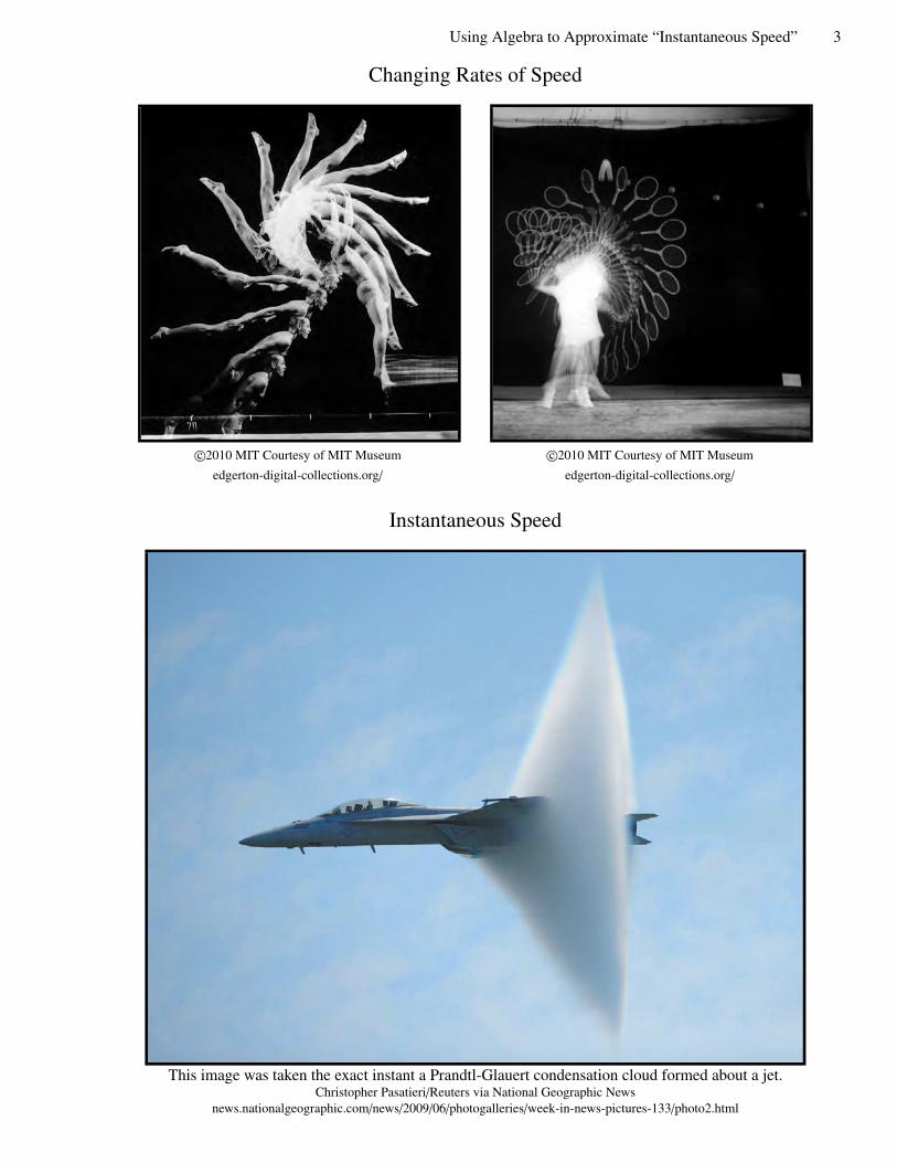
Changing Rates of Speed

c�2010 MIT Courtesy of MIT Museum c�2010 MIT Courtesy of MIT Museumedgerton-digital-collections.org/ edgerton-digital-collections.org/

Instantaneous Speed

This image was taken the exact instant a Prandtl-Glauert condensation cloud formed about a jet.Christopher Pasatieri/Reuters via National Geographic News

news.nationalgeographic.com/news/2009/06/photogalleries/week-in-news-pictures-133/photo2.html


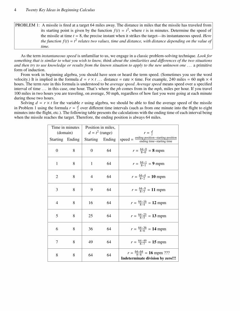
PROBLEM 1: A missile is fired at a target 64 miles away. The distance in miles that the missile has traveled fromits starting point is given by the function f (t) = t2, where t is in minutes. Determine the speed ofthe missile at time t = 8, the precise instant when it strikes the target—its instantaneous speed. Herethe function f (t) = t2 relates two values, time and distance, with distance depending on the value oftime.

As the term instantaneous speed is unfamiliar to us, we engage in a classic problem-solving technique. Look forsomething that is similar to what you wish to know, think about the similarities and differences of the two situationsand then try to use knowledge or results from the known situation to apply to the new unknown one . . . a primitiveform of induction.

From work in beginning algebra, you should have seen or heard the term speed. (Sometimes you see the wordvelocity.) It is implied in the formula d = r × t . . . distance = rate × time. For example, 240 miles = 60 mph × 4hours. The term rate in this formula is understood to be average speed. Average speed means speed over a specifiedinterval of time . . . in this case, one hour. That’s where the ph comes from in the mph, miles per hour. If you travel100 miles in two hours you are traveling, on average, 50 mph, regardless of how fast you were going at each minuteduring those two hours.

Solving d = r × t for the variable r using algebra, we should be able to find the average speed of the missilein Problem 1 using the formula r = d

t over different time intervals (such as from one minute into the flight to eightminutes into the flight, etc.). The following table presents the calculations with the ending time of each interval beingwhen the missile reaches the target. Therefore, the ending position is always 64 miles.

Time in minutes(domain)

Position in miles,d = t2 (range) r = d

t

Starting Ending Starting Ending speed = ending position−starting positionending time−starting time

0 8 0 64 r = 64−08−0 = 8 mpm

1 8 1 64 r = 64−18−1 = 9 mpm

2 8 4 64 r = 64−48−2 = 10 mpm

3 8 9 64 r = 64−98−3 = 11 mpm

4 8 16 64 r = 64−168−4 = 12 mpm

5 8 25 64 r = 64−258−5 = 13 mpm

6 8 36 64 r = 64−368−6 = 14 mpm

7 8 49 64 r = 64−498−7 = 15 mpm

8 8 64 64 r = 64−648−8 = 16 mpm ???

Indeterminate division by zero!!!


The sequence of average speeds calculated above, 8 mpm, 9 mpm, 10 mpm, 11 mpm, 12 mpm, 13 mpm, 14 mpmand 15 mpm, seems reasonable as we know from watching tv and movies that rocket ships get faster and faster asthe initial stationary inertia of the projectile is overcome by the rocket’s thrust. Did we achieve our goal of obtainingthe instantaneous speed of the rocket at t = 8 or equivalently at d = 64? Well, no, but we suspect that it must begreater than 15 mpm.

Let us continue this same pattern of analysis. Let’s concentrate on the average speed as the missile approachesits target over the last minute (t = 7 to t = 8) of its flight: f (t) = t2.



t


7 8 49 64 r = 64−498−7 = 15 mpm

7.9 8 62.41 64 r = 64−62.418−7.9 = 15.9 mpm

7.99 8 63.8401 64 r = 64−63.84018−7.99 = 15.99 mpm

7.999 8 63.984001 64 r = 64−63.9840018−7.999 = 15.999 mpm

8 8 64 64 r = 64−648−8 = 16 mpm ???


Combining the old data for average speeds as the missile approached its target with the new data for averagespeeds, we now get the sequence of “average speeds” as calculated above for decreasing intervals of time:

8, 10, 12, 14, 15, 15.9, 15.99, and 15.999

From the pattern of average speeds shown above, it would seem reasonable to conclude that the “instantaneousspeed” when t = 8 minutes and d = 64 miles is 16 mpm. However, how could you justify or prove such ananswer? The answer is, “Using simple algebraic skills you can’t.” You can only approximate. (See Appendix A,15.999 . . . = 16, for an interesting discussion of this.) The algebraic attempt to calculate the instantaneous speedusing the formula for average speed over a time interval of zero length results in a division by zero. The proof thatthe instantaneous speed of the missile at t = 8 seconds and d = 64 miles is exactly 16 mpm can only be obtainedusing knowledge and skills and vocabulary learned in calculus.


OK let’s review.

PROBLEM 1: A missile is fired at a target 64 miles away. The distance in miles that the missile has traveled fromits starting point is given by the function f (t) = t2, where t is in minutes. Determine the speed of themissile at time t = 8, the precise instant when it strikes the target—its instantaneous speed.

The sequence of “average speeds” as calculated above for decreasing intervals of time is:

8, 10, 12, 14, 15, 15.9, 15.99, and 15.999 . . . 16 mpm ???

We suspect that the “instantaneous speed” for the missile when t = 8 minutes and d = 64 miles is 16 mpm butcannot really prove our suspicions. Look at the sequence of average speeds again. How would you describe them?Are they getting larger with each term? Yes. Could an average speed ever get to be 100 mpm? Do you think thatgiven the function f (t) = t2 and the time and distance constraints (0 <= t <= 8 minutes, 0 <= d <= 64 miles) thatthe missile will ever speed up to 100 mpm in its last 0.001 minute of flight? Do you think that the instantaneousspeed will ever get larger than 16? Do you think that the instantaneous speed will ever reach 16? Let’s look at thosenumbers one more time:

(average speeds over decreasing time intervals)8, 10, 12, 14, 15, 15.9, 15.99, 15.999 mpmˆ ˆ ˆ ˆ ˆ ˆ ˆ2 2 2 1 0.9 0.09 0.009

(increase of average speed from the previous time interval)

After one month of instruction, a cal-

culus student should be able to solve

for the exact answer to Problem 1 in-

side the space of this text box and be

able to do so in less than a minute.

These numbers (average speeds) are increasing each for each interval, but the rate ofincrease each time seems to be decreasing with the decreasing time intervals. Basedon the pattern of speed increases shown above, the last speed of 15.999 mpmover the last 0.001 minute of flight will probably not increase greatly duringthe remaining time of the missile’s flight. It appears that the number16 acts as a sort of barrier or limit to the progression ofnumbers we are calling average speeds. The studyof calculus will give you the tools to justifythis suspicion. It will allow you to say, with-out any doubt, that the instantaneous speed of themissile in this question at t = 8 minutes is 16 mpm.


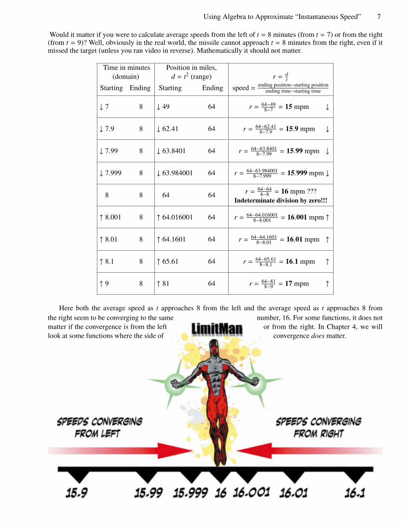
Would it matter if you were to calculate average speeds from the left of t = 8 minutes (from t = 7) or from the right(from t = 9)? Well, obviously in the real world, the missile cannot approach t = 8 minutes from the right, even if itmissed the target (unless you ran video in reverse). Mathematically it should not matter.



t


↓ 7 8 ↓ 49 64 r = 64−498−7 = 15 mpm ↓

↓ 7.9 8 ↓ 62.41 64 r = 64−62.418−7.9 = 15.9 mpm ↓

↓ 7.99 8 ↓ 63.8401 64 r = 64−63.84018−7.99 = 15.99 mpm ↓

↓ 7.999 8 ↓ 63.984001 64 r = 64−63.9840018−7.999 = 15.999 mpm ↓

8 8 64 64 r = 64−648−8 = 16 mpm ???


↑ 8.001 8 ↑ 64.016001 64 r = 64−64.0160018−8.001 = 16.001 mpm ↑

↑ 8.01 8 ↑ 64.1601 64 r = 64−64.16018−8.01 = 16.01 mpm ↑

↑ 8.1 8 ↑ 65.61 64 r = 64−65.618−8.1 = 16.1 mpm ↑

↑ 9 8 ↑ 81 64 r = 64−818−9 = 17 mpm ↑

Here both the average speed as t approaches 8 from the left and the average speed as t approaches 8 fromthe right seem to be converging to the same number, 16. For some functions, it does notmatter if the convergence is from the left or from the right. In Chapter 4, we willlook at some functions where the side of convergence does matter.


A function f (x) can be vertically shifted by k, giving f (x) + k. The slopes of the tangents to function f (x) andthe new function f (x) + k at any point x will be the same: d

dx [ f (x)] = ddx [ f (x) + k]. This is true whether the vertical

shift is up or down: ddx [ f (x)] = d

dx [ f (x) − k].

!!"!"##$!%!$

$

%&!"!%'

!!"!"##$

%&

#

%'

!!"!"##$

$ %(!"!%)

!!"!"##$!*!$

%(

#

%)

When a function f (x) is multiplied by a constant k, k[ f (x)], the slope of the tangent to the function, k[ f (x)], willbe k times the slope of the tangent to the function f (x).

!!"!"##$$

%%!"!"%&%'!"!"%(

%)!"!"%*

!!"!##$$

%%

%'

$' $% $*

%(%&

%)

%*

At any point x, the slope of the tangent to the curve k[ f (x)] is k times the slope of the tangent to the curve f (x):ddx [k f (x)] = k

�ddx [ f (x)]

�.

! " # $

%&''()*+&+,

-./01'2

!)3)""!$

!4

5

"

!5

!"

6

$

“I’d like to be your derivative so I could lay next to your curves.”The Big Bang Theory, a tv show about

geeky, socially awkward scientists.

“I’d like to be your integral so I could fill in your spaces.”The Big Bang Theory, a tv show about

geeky, socially awkward scientists.

Min and Max Problems, Another “Generic Problem Set” 97

Chapter 10 Review

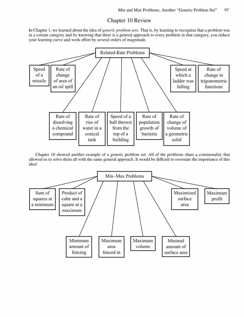
In Chapter 1, we learned about the idea of generic problem sets. That is, by learning to recognize that a problem wasin a certain category and by knowing that there is a general approach to every problem in that category, you reduceyour learning curve and work effort by several orders of magnitude.

Related-Rate Problems

Speedof amissile

Rate ofchangeof area ofan oil spill

Rate ofchange ofvolume ofa geometricsolid

Rate ofchange in

trigonometricfunctions

Rate ofdissolvinga chemicalcompound

Speed of aball thrownfrom thetop of abuilding

Speed atwhich aladder wasfalling

Rate ofpopulationgrowth ofbacteria

Rate ofrise ofwater in aconicaltank

Chapter 10 showed another example of a generic problem set: All of the problems share a commonality thatallowed us to solve them all with the same general approach. It would be difficult to overstate the importance of thisidea!

Min–Max Problems

Sum ofsquares ata minimum

Product ofcube and asquare at amaximum

Maximizedsurfacearea

Maximumprofit

Minimumamount offencing

Maximumarea

fenced in

Maximumvolume

Minimalamount ofsurface area


On the lead-in page to Chapter 10, we saw this nifty figure courtesy of my editor. It shows that whenever afunction is at a local minimum or maximum, the derivative at that x value is equal to 0.

! !""#$%$&

! !"'#$%$&

#$%$!!"#

! !"(#$%$&

"("' """) "* "+

! !"*#$%$&

! !"+#$%$&

,-./,0/1

,-./,0/1

23456370/1

2-7042

! !")#$%$&

23456370/1

2-7042

,-./,042

,-./,042

Another way to look at this information is to remember that the term “derivative” is actually a short way of saying“derivative function.” You may remember in Chapter 1 that a derivative was referred to as a “derivative (function).”

f (x) = xn f �(x) = nxn−1

f (x) =13

x3 − 2x2 + x + 9 f �(x) =13

�3x3−1

�− 2�2x2−1

�+ 1�x1−1�+ 0

= x2 − 4x + 1

Below we see the two functions f (x) and f �(x) graphed side by side.

!" # $ %&!&% &$ &# &"

#$'(")"#"$"'"(#)###$

&(&")

&'&$&#

!*"+,-,,,"!,&,#"#,.,",.,/!"

!" # $ %&!&% &$ &# &"

#$'(")"#"$"'"(#)###$

&(&")

&'&$&#

! *"+,-,"#,&,$",.,"

0123456341

Min and Max Problems, Another “Generic Problem Set” 99

Finally, we see the two functions f (x) and f �(x) superim-posed on the same axes.

!!""#$###"%#&#'"'#(#"#(#)%*

%* ' + ,&%&, &+ &' &*

'+-.*/*'*+*-*.'/'''+

&.&*/

&-&+&'

! !""#$#"'#&#+"#(#*

f �(x) = 0 when f (x) is at a local max or min.

The x-intercept for a function occurs whenever the func-tion crosses the x-axis—when the y value equals 0. The x-intercepts of the derivative (function), f �(x) = x2−4x+1,are shown at right as Points 1 and 2. Notice that the func-tion f (x) is at a local maximum at Point 1 and at a localminimum at Point 2.

!!""#$###"%#&#'"'#(#"#(#)

*+,-./.

%0

%0 ' 1 2&%&2 &1 &' &0

'134050'010304'5'''1

&4&05

&3&1&'

! !""#$#"'#&#1"#(#0

*-6-./.

"#-6789:8;7<

0

0

'

'


This was taught previously using a graphic comparable tothe the graph at right.

!" # $ %&!&% &$ &# &"

#$'(")"#"$"'"(#)###$

&(&")

&'&$&#

!*"+,-,,,"!,&,#"#,.,",.,/!"

! *"+,-,)! *"+,-,)



Chapter 11 Lead In

In calculus, it is frequently the case that there are two different ways of looking at the same information. This wasshown in Chapter 2 when we found that “instantaneous speed” was mathematically equivalent to “slope of a tangentto a curve at a given point.” In Chapter 11, we will again be seeing that the same information can be viewed fromtwo different perspectives. The ability to see the same idea from two different perspectives is very, very helpful inthe study of calculus. This ability comes so naturally to your calculus teacher that he or she may not point this out toyou. He or she will assume that if you understand one of two equivalent ideas that you understand the other.

Chapter 2 emphasized an important concept: For functions of the form y = f (x), an average speed between twopoints in time, (a, f (a)) and (b, f (b)), could be obtained using the formula f (b)− f (a)

b−a . Alternatively, the slope of a secantline between two points, (x1, y1) and (x2, y2), on a function could be found using the formula m = y2−y1

x2−x1. Although

these were two different interpretations of the data, they were both mathematically equivalent. This equivalenceallowed us to interchange ideas between a conceptual (real-world) problem and a graph. Chapter 4 presented adefinition, “The Definition of f �(x),” that allowed us to decrease the interval between the two points in time (or thetwo points used to determine secant slope) down to zero, allowing us to find either the “instantaneous speed” or the“slope of a tangent” at a given point. Either process could be referred to by the generic term “finding a derivative.”

All the problems in Chapters 1–10 involved rates of change and were representative of the branch of calculusknown as differential calculus. Chapter 11 begins the study of a different branch of calculus, integral calculus. Aswith differential calculus, the doorway to this branch of calculus will be a definition, The Definition of Area Undera Curve. Again, as with differential calculus, there will be a mathematical equivalence between a real-world conceptand a mathematical one. This equivalence will again allow us to interchange ideas between a conceptual (real-world)problem and a graph.

Two different ways of looking at the same idea.

Specifically, in Chapters 11 and 12, we will find that the area under a curve is equivalent to finding how much“distance was traveled,” “pressure is exerted,” “work occurred,” etc.

1.) A rocket is accelerating (speeding up). Its speed (in mpm) is given by the function r = t2. How far did the

rocket travel in the first four minutes? In general this problem is worked using the formula Distance = rate× time or d = rt.

2.) Given that the density of water is 62.5 lb/ft3, find the force of the water against a triangular dam 50 feet

wide and 40 feet deep. In general, this problem is worked using the formula pressure = force × area or p = f a.

3.) A force of 500 pounds compresses a spring 2 inches from its natural length of 16 inches. Use Hooke’s Law,

f = kd, to find the work done in compressing the spring an additional four inches. In general, thisproblem is worked using the formula Work = Force × Distance or w = f d.

Chapter 11Using Algebra to Introduce Integral Calculus

A car travels 10 mph for one hour20 mph for one hour30 mph for one hour

and 40 mph for one hourWhat was the total distance that the car traveled?

Total distance the car traveled = d1+d2+d3+d4.This total distance can be thought of in two differentways as shown below.

1 2 3 4

10

20

30

40

Speed

Hours

10 miles

traveled

20 miles

traveled

30 miles

traveled

40 miles

traveled

(Using the distance formula, d = rt)

dhour 1 + dhour 2 + dhour 3 + dhour 4 =

Note that distance is rate times time: d = rt(r1t1) + (r2t2) + (r3t3) + (r4t4) =

(10 × 1) + (20 × 1) + (30 × 1) + (40 × 1) =10 + 20 + 30 + 40 = 100 miles

(Using the area of a rectangle formula, a = bh)

dhour 1 + dhour 2 + dhour 3 + dhour 4 =

Note that area is base times height: d = a = bh(b1h1) + (b2h2) + (b3h3) + (b4h4) =

(10 × 1) + (20 × 1) + (30 × 1) + (40 × 1) =10 + 20 + 30 + 40 = 100 miles

It is more than just a little bit important for you to understand what is demonstrated above. The thought processat the left uses the formula d = rt and shows how a science or engineering teacher thinks. The thought process atthe right uses the formula a = bh and shows how a mathematics teacher thinks. These two ways of thinking aboutthe problem are mathematically equivalent: The width of the base of each rectangle is equal to the time the carspends traveling at each speed. Correspondingly, the height of each rectangle is equal to the rate at which the carwas traveling.

Math teachers teach in generalities using abstractions assuming that their students understand that such skillscan be applied to specific problems in business, science, engineering, psychology, and many other fields. But thegeneralities that math teachers use are sometimes very far removed from any application, so far that the studentmight miss the connection between the two.

101


A rocket is accelerating (speeding up). Its speed (in mpm) is given by the functionr = t2. How far did the rocket travel in the first 4 minutes?

r = t2

Time (minutes) Speed (mpm)0 01 12 43 94 16

This new problem is pretty well the same as the one before except for the fact that the object in motion isnow moving with a continuous acceleration. Before, because the car’s speed over each of the equally spaced timeintervals was constant and because the change in speed was effectively instantaneous each time the speed did change,we could represent the distance traveled over each time interval as the area of a rectangle and calculate the respectiveareas (distance traveled over each time interval). The fact that this new problem is conceptually the same as theprevious one means that the answer to the new problem could be found by finding the area under the curve fromx = 0 to x = 4. However, this time we have a continuous and variable speed, resulting in a curved line which willnot allow us to form and add up areas/distances using the formulas d = rt and a = bh. Conceptually, there aresimilarities here to Chapters 1 and 2 in this book. There, we did not know how to find instantaneous speed or slopeof a tangent to a curve at a given point, so we used our algebra skills to generate successive approximations of thedesired information, r = d

t and m = y2−y1x2−x1

. That gives us the idea of successively approximating the area under thecurve by adding up an increasing number of smaller and smaller rectangle areas.

As has been shown on the previous page, each of the four rectangle areas shown here approximates the distancethe rocket traveled over that time interval. (Author’s note, partition 0 is from 0 to 1. Note also that the y axis iscompressed in the graph below.)

! " # $

%&''()*+&+,

-./01'2

!)3)""

4)+.5'21678'5'(

!)+.5'1678'5'(

!$

!4

9

"

!9

!"

:

$$)+.5'21678'5'(

;)+.5'21678'5'(

The distance that the rocket traveled over four minutes is approximately 14 miles (0 + 1 + 4 + 9). Notice thatthe rectangles do not completely fill the space below the curve. There are four rounded triangles missing from thecalculated area below the curve y = x2. That means that this is a low estimate.

xRectangle height

x2Rectangle base (interval/number

of rectangles)Area of the rectangle

a = bh0 0 1 01 1 1 12 4 1 43 9 1 9

Using Algebra to Introduce Integral Calculus 103

To improve the previous approximation, we next increasethe number of rectangular partitions to eight. Now the base ofeach rectangle is the size of the interval divided by the numberof partitions = 4

8 =12 . (Author’s note, partition 0 is from 0 to 1

2 .Note also that the y axis is compressed.) The sum of these eightrectangle areas is 0+ 1

8 +48 +

98 +

168 +

258 +

368 +

498 =

1408 = 17.5

units.

xRectangle height

x2Rectangle base

intervalnumber of rectangles

Area of therectangle a = bh

0 0 12 0

12

14

12

18

1 1 = 44

12

12 =

48

32

94

12

98

2 4 = 164

12 2 = 16

852

254

12

258

3 9 = 364

12

92 =

368

72

494

12

498

Let’s talk about those units for a moment. The base

of the rectangle is minutes (min), and the height of the

rectangle is miles per minute

�miles

min

�. So, the product is

miles

✟✟min×✟✟✟min = miles. That’s good; the units match what we

thought we were calculating.

Therefore, the distance the rocket traveled over four min-utes is approximately 17.5 miles. Continuing this pattern for16 and 32 rectangles, we get the figures at right.

! " # $

%&''()*+&+,

-./01'2

!)3)""!$

!4

5

"

!5

!"

6

$

! " # $

%&''()*+&+,

-./01'2

!)3)""!$

!4

5

"

!5

!"

6

$

! " # $

%&'()*+

,+-

./+()*+/0-

!)1)""!$

!2

3

"

!3

!"

4

$

56)#)/078(&6(69)$%):('6)7;<6(8)

'<)'=()&7'>&;)&8(&)>0?(8)'=()7>8@(

#&A&!

2

The mathematics of adding up these areas is getting more laborious and time consuming. Perhaps there is apattern we could use. Using the data from the table, let’s sum up the areas of the graph with eight rectangles.

Area = 0 +18+

48+

98+

168+

258+

368+

498=

1408= 17.5

= area0 + area1 + area2 + area3 + area4 + area5 + area6 + area7 = total area

= b0h0 + b1h1 + b2h2 + b3h3 + b4h4 + b5h5 + b6h6 + b7h7

Now, since the base of all these rectangles is the same— interval lengthnumber of rectangles —substitute b for bn:

Area = bh0 + bh1 + bh2 + bh3 + bh4 + bh5 + bh6 + bh7

= b × (h0 + h1 + h2 + h3 + h4 + h5 + h6 + h7), factor out b

=12×0

2 +

�12

�2+

�22

�2+

�32

�2+

�42

�2+

�52

�2+

�62

�2+

�72

�2

=12×�0 +

14+

44+

94+

164+

254+

364+

494

�=

12× 1

4× [0 + 1 + 4 + 9 + 16 + 25 + 36 + 49], factor out

14

=18×�02 + 12 + 22 + 32 + 42 + 52 + 62 + 72

�=

18× the sum of the squares of the integers from 0 to 7

=18× 7 × 8 × 15

6= 17.5, a formula from precal states

n−1�

0

i2 =(n − 1)(n)(2n − 1)

6, see Appendix H


In general, this work suggests that the area of any n rectangles could be found by the formula b3× (n−1)(n)(2n−1)6 =

� interval lengthnumber of rectangles

�3 × (n−1)(n)(2n−1)6 . Note that this only works to approximate the area under the curve y = x2 on the

interval from zero to four.

16 rectangles, on [0, 4] :�

416

�3× 15 × 16 × 31

6=

15 × 16 × 3164 × 6

= 19.375


432

�3× 31 × 32 × 63

6=

31 × 32 × 63512 × 6

= 20.34375


464

�3× 63 × 64 × 127

6=

63 × 64 × 1274,096 × 6

= 20.8359375


4128

�3× 127 × 128 × 255

6=

127 × 128 × 25532,768 × 6

= 21.0839843


4256

�3× 255 × 256 × 511

6=

255 × 256 × 511262,144 × 6

= 21.2084961

Number ofpartitions

Rectanglesum

4 148 17.5

16 19.37532 20.3437564 20.8359375

128 21.0839843256 21.2084961

The table and calculations above going up to 256 partitions suggest the rectangular sum will continue to getlarger; as it does, more and more of the area under the curve will be included in the summation process. Does it seemas though the summation of the rectangles could ever be as much as 100? Could there ever be enough rectangles?The rectangles are getting more and more numerous, but each of their areas is getting smaller. That is what theprocess called “exhaustion” does. It “exhausts” more and more of the unused areas under the curve and the result isthat the sum of rectangle areas is getting closer and closer to the area under the curve. See the figures on page 103.

What would happen if we approached the area under the curve from the other direction, upper approximationsgetting closer and closer to the actual area? See the figure below. As before, the y-axis has been compressed fordemonstration purposes.

! " # $

%&''()*+&+,

-./01'2

!)+.3'1456'3'(

$)+.3'21456'3'(

!$

!7

8

"

!8

!"

9

$

:)+.3'21456'3'(

!8)+.3'21456'3'(!);)""

xRectangle height

x2Rectangle base


Area of the rectanglea = bh

1 1 1 12 4 1 43 9 1 94 16 1 16

The sum of the four rectangles is 1 + 4 + 9 + 16 = 30 units. The distance that the rocket traveled over fourminutes is approximated to be 30 miles. Clearly this approximation is high as there are areas above the curve thatwere included in this approximation and should not have been.

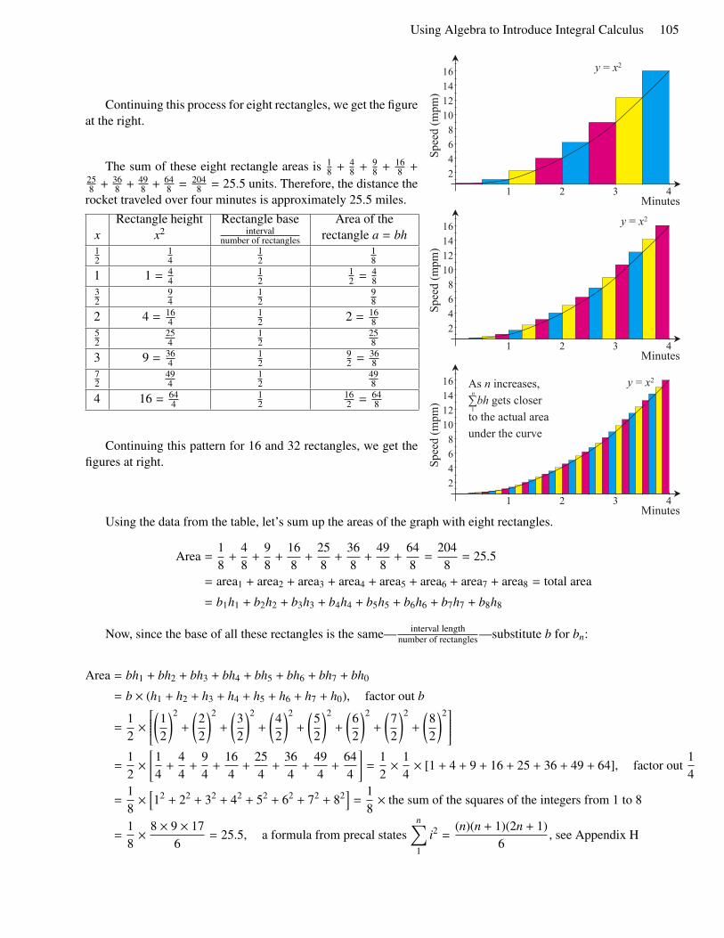
Using Algebra to Introduce Integral Calculus 105

Continuing this process for eight rectangles, we get the figureat the right.

The sum of these eight rectangle areas is 18 +

48 +

98 +

168 +

258 +

368 +

498 +

648 =

2048 = 25.5 units. Therefore, the distance the

rocket traveled over four minutes is approximately 25.5 miles.

xRectangle height

x2Rectangle base


Area of therectangle a = bh

12

14

12

18

1 1 = 44

12

12 =

48

32

94

12

98

2 4 = 164

12 2 = 16

852

254

12

258

3 9 = 364

12

92 =

368

72

494

12

498

4 16 = 644

12

162 =

648

Continuing this pattern for 16 and 32 rectangles, we get thefigures at right.

! " # $

%&''()*+&+,

-./01'2

!$

!3

4

"

!4

!"

5

$

!)6)""

! " # $

%&''()*+&+,

-./01'2

!)3)""

!$

!4

5

"

!5

!"

6

$

! " # $

%&''()*+

&+,

-./01'2

!)3)""!$

!4

5

"

!5

!"

6

$

72)#)./89':2'2;)$%)<'12)8=>2'9)

1>)1?'):810:=):9':)0/('9)1?')809@'

#

!

Using the data from the table, let’s sum up the areas of the graph with eight rectangles.

Area =18+

48+

98+

168+

258+

368+

498+

648=

2048= 25.5

= area1 + area2 + area3 + area4 + area5 + area6 + area7 + area8 = total area

= b1h1 + b2h2 + b3h3 + b4h4 + b5h5 + b6h6 + b7h7 + b8h8

Now, since the base of all these rectangles is the same— interval lengthnumber of rectangles —substitute b for bn:

Area = bh1 + bh2 + bh3 + bh4 + bh5 + bh6 + bh7 + bh0

= b × (h1 + h2 + h3 + h4 + h5 + h6 + h7 + h0), factor out b

=12×

�12

�2+

�22

�2+

�32

�2+

�42

�2+

�52

�2+

�62

�2+

�72

�2+

�82

�2

=12×�14+

44+

94+

164+

254+

364+

494+

644

�=

12× 1

4× [1 + 4 + 9 + 16 + 25 + 36 + 49 + 64], factor out

14

=18×�12 + 22 + 32 + 42 + 52 + 62 + 72 + 82

�=

18× the sum of the squares of the integers from 1 to 8

=18× 8 × 9 × 17

6= 25.5, a formula from precal states

n�

1

i2 =(n)(n + 1)(2n + 1)

6, see Appendix H


In general, this work suggests that the area of any n rectangles could be found by the formula b3× (n)(n+1)(2n+1)6 =

� interval lengthnumber of rectangles

�3 × (n)(n+1)(2n+1)6 . Note that this only works to approximate the area under the curve y = x2 on the

interval from zero to four.


416

�3× 16 × 17 × 33

6=

16 × 17 × 3364 × 6

= 23.375


432

�3× 32 × 33 × 65

6=

32 × 33 × 65512 × 6

= 22.3437


464

�3× 64 × 65 × 129

6=

64 × 65 × 1294,096 × 6

= 21.8359375


4128

�3× 128 × 129 × 257

6=

128 × 129 × 25732,768 × 6

= 21.5839844


4256

�3× 256 × 257 × 513

6=

256 × 257 × 513262,144 × 6

= 21.4584961

Number ofpartitions

Lowerrectangle

sum

Upperrectangle

sum4 14 308 17.5 25.5

16 19.375 23.37532 20.34375 22.343764 20.8359375 21.8359375

128 21.0839843 21.5839844256 21.2084961 21.4584961

Are you getting another one of those deja vu feelings? Something seems familiar here.

Reorganizing the current area sum data from the table shown above as we did when approximating instantaneousspeeds in the Chapter 1 review, we get the following table.

Lower area rectangles Upper area rectanglesNumber ofrectangles

64 → 128 → 256 → ∞ ← 256 ← 128 ← 64

Area sum ofrectangles

20.83594 → 21.08398 → 21.208496 → Actual areaunder curve

← 21.458496 ← 21.58398 ← 21.83594

Limit of an Infinite Series

Now it is more clear that the lower area rectangle sums are increasing toward the area under the curve y = x2

from below while the upper area rectangle sums are decreasing toward the same value (area under the curve) fromabove. The upper and lower sums are approaching the same value—a limit. That limit is the area under the curve.

This is all very similar to the discussion and table in Chapter 1 when we showed secant-line slopes as theyapproached the slope of the tangent to the curve y = x2 at x = 8 from both the right and the left. That tangent slopeof 16 limited the progression of secant slopes from both the left and the right. Remember LimitMan in Chapter 1?

x 7.9 → 7.99 → 7.999 → 8.0 ← 8.001 ← 8.01 ← 8.1m 15.9 → 15.99 → 15.999 → 16.0??? ← 16.001 ← 16.01 ← 16.1

Limit of an infinite Sequence of Secant Slopes

In Appendix B, we will see a new kind of limit, the limit of a function.


In order for the rectangles to perfectly fit under the curve they will all need to be very skinny and there will needto be a lot of them. Intuitively you can think of this situation as “infinite rectangles, each infinitesimally narrow.”


64 → 128 → 256 → ∞ ← 256 ← 128 ← 64


63�i=0

f (xi)∆x →127�i=0

f (xi)∆x →255�i=0

f (xi)∆x → Actual areaunder curve ←

256�i=1

f (xi)∆x ←128�i=1

f (xi)∆x ←64�i=1

f (xi)∆x

The lower area rectangle sums are increasing toward the area under the curve y = f (x) from below whilethe upper area rectangle sums are decreasing toward the same value (area under the curve) from above. The mathsymbolism used when that happens is

limn→∞

n−1�

i=0

li∆x = limn→∞

n�

i=1

ui∆x,

where li represents the lengths of all rectangles “lower than” the curve and ui represents the lengths of all the“upper” rectangles, ∆x represents the width of each rectangle in each set and is determined by the expressionupper domain−lower domain

number of partitions , n is the number of rectangles being summed in this set, and i is a counter that keeps track ofwhich rectangle you are summing.

There is something to keep in mind. It canbe demonstrated that when n → ∞, it reallydoes not matter too much whether the area isapproached using lower sums or using uppersums or rectangles that are partly above andpartly below. To see this, note that the heightof the rectangle is significantly affected by thischoice when the width of the rectangle is large,but it is not significantly affected by this choicewhen the width of the rectangle is small. Thefigure at right can help clarify this point.

All this implies that you can choose any xvalue in the ith subinterval and that choice willnot affect the limit (sum of areas) when n→ ∞.

!!"!"##$

#%&'('!$%!)!$!)!$% $$$!"!& $!"!'

$$% $$%

*'+,!-.(/'(

012&,!-.(/'(31445'

67 8 9 : ;<=

6

7

8

>7

9

:

77? 7@ 78

The lower and upper sum limits,

limn→∞

n−1�

i=0

f (li)∆x = limn→∞

n�

i=1

f (ui)∆x,

can be seen in the definition at right.

Definition of Area Under a CurveLet f be continuous and nonnegative on the interval [a, b]. The area of the

region bounded by f , the x-axis, and the vertical lines x = a and x = b, is

limn→∞

n�

i=1

f (xi)∆x,

where a < xi < b, with i designating the subinterval of x and ∆x = b−an .

Calculus with Analytic Geometry (5th ed.) Larson, Hostetler, and Edwards,D.C. Heath, 1994, pg. 265, modified by this author.

Let’s try this new definition out on the problem in Chapter 11!

A rocket is accelerating (speeding up). Its speed(in mpm) is given by the function r = t2. How fardid the rocket travel in the first 4 minutes?

! " # $

%&''()*+&+,

-./01'2

!)3)""!$

!4

5

"

!5

!"

6

$

Infinite Summations, Definition of “Area Under a Curve” 111

limn→∞

n�

i=1

f (xi)∆x = limn→∞

�interval lengthnum rectangles

�3 n(n + 1)(2n + 1)6

, from work done in Chapter 11

= limn→∞

�4n

�3 n(n + 1)(2n + 1)6

= lim

n→∞

�64n3

n(n + 1)(2n + 1)6

�, because

�ab

�m=

am

bm

= limn→∞

�64n2

(n + 1)(2n + 1)6

�, canceling out the n terms

= limn→∞

�32n2

2n2 + n + 2n + 13

�, reducing

646

to323

and FOIL

= limn→∞

�32n2

2n2 + 3n + 13

�= lim

n→∞

�64n2 + 96n + 32

3n2

�

= limn→∞

64n2

3n2 + limn→∞

96n3n2 + lim

n→∞323n2 , limit of a sum is the sum of the its limits

= limn→∞

643+ 0 + 0, canceling

n2

n2 and reducing96n3n2 , then the denominators go to∞

= 21.333333, actual area under the curve!

Let’s compare this answer with the lower and upper sum approximations we obtained back in Chapter 11 whenwe were doing this same problem. As the number of rectangles goes to infinity, the sum of areas goes to the areaunder the curve.


64 → 128 → 256 → ∞ ← 256 ← 128 ← 64


20.83594 → 21.08398 → 21.208496 → 21.333333 ← 21.458496 21.58398 ← 21.83594

Without calculus With integral calculus

a1 + a2 + · · · + an = S a1 + a2 + · · · = S

Sum of a finite number of terms Sum of an infinite number of terms


Chapter 12 Review

In Chapter 12, attempts to determine the area undera curve using successive approximation of finite rectangleareas are replaced with the summation of infinite rectangleareas allowing us to find the area under a curve exactlyrather than approximately. Just as in Chapter 4, where theDefinition of f �(x) allowed us to find an exact value forthe slope of a tangent to a curve,

!"#$%$&$'%('#(! )"*

! )"*(+(,$-# "

!)"*(.(!)#*"(.(#

/0"(1'-2$%('#(! )"*($3(&0"(3"&(4'%3$3&$%5('#("6"78(%9-:"7;("$(2&(<0$40(&0"(2:'6"(,$-$&("=$3&3>

?@

AB

Johnson and Kiokemeister’s Calculus with AnalyticGeometry (5th ed.), Johnson, Kiokemeister, and Wolk,Allyn and Bacon, 1974, pg. 91, modified by this author.

the new definition of the areaunder a curve,

Definition of Area Under a CurveLet f be continuous and nonnegative on the interval [a, b]. The area of the

region bounded by f , the x-axis, and the vertical lines x = a and x = b, is

limn→∞

n�

i=1

f (xi)∆x,

where a < xi < b, with i designating the subinterval of x and ∆x = b−an .

Calculus with Analytic Geometry (5th ed.) Larson, Hostetler, and Edwards,D.C. Heath, 1994, pg. 265, modified by this author.

allows us to find an exact value for the area under a curve. This new definition was demonstrated by applying it tothe problem that was worked back in Chapter 11. Intuitively, the “Definition of Area Under a Curve” can be thoughtof as summing up the areas of infinitesimally thin rectangles. Both of these definitions involve the idea of “limit.” Inthis book, we see three kinds of limits: limit of a sequence of secant slopes, limit of a series, and limit of a function.

!!" "

"!"!##$$!%!##%$

&'()!#('*$

+',-.*/)!#('0),$ #$1!##$$$

#%1!##%$$

&

&!"!$!%!%

"!"!&2 “A missile is accelerating. Its distance is given by the function d =t2. Find the instantaneous speed of the missile when it strikes itstarget at t = 4.” The definition of f

�(x) is applied here to find

the limit of an infinite sequence of ratios. (Recall that d = rt sor = d/t.) As n→ ∞, d1

t1 ,d2t2 ,

d3t3 ,

d4t4 . . .→ r, the instantaneous speed

at t.

!"#$%&'()'(*+(+,

-.//$&$"#.'()'(*+(+,

! " # $

%&'()*+

,+-

./+()*+/0-

!)1)""!$

!2

3

"

!3

!"

4

$

56)#)/078(&6(69)$%):('6)7;<6(8)

'<)'=()&7'>&;)&8(&)>0?(8)'=()7>8@(

#&A&!

2

“A missile is accelerating. Its speed is given by the function r = t2.Find the distance the missile traveled at t = 4.” The definition

of “area under a curve” is applied here on the same three

variables as were used in the problem above (d, r, and t) to

find the limit of an infinite series of products. As n → ∞,r1t1 + r2t2 + r3t3 + r4t4 + · · · → d. (Recall from pg 103 thatr × t = miles

✟✟min ×✟✟min = miles.) The definition of f � generates aninfinite “sequence,” while the definition of area under a curve gen-erates an infinite “series.”


Since calculating the area under a curve is mathematically equivalent to solving many applied problems, thisskill takes on new importance and significance. Finding the area under the curve y = x2 was easy because that par-ticular problem involved summing up perfect squares,

�ni=1 i2. A clever formula (Appendix H) was used to develop

another formula, interval lengthnumber of rectangles

n(n+1)(2n+1)6 . In general, the functions we will be using will not lend themselves to

the development of such clever formulas. Even if they did, there is an infinity of function possibilities, and it wouldnot be desirable to have to develop a special formula for each of them. What we need is a generic approach that willwork for all functions. That is what Chapter 13, and the Fundamental Theorem of Calculus, is about.

The goal of the Fundamental Theorem of Calculus is to develop a function that will allow a person to obtainthe area under a curve simply by substituting values a and b into that function. This function, Area(a, b), will beanalogous to the previously discussed f �(x) that allows us to quickly and simply evaluate the instantaneous speed orslope of a tangent to a polynomial curve at a specified point (x, f (x)).

Function machine to determine slope of the tangentto a function at any point (x, f (x)) on the function.

No more using secant-line slopes to successivelyapproximate the slope of a tangent.

Function machine to determine the area undera curve between specified bounds, a ≤ x ≤ b.

No more using rectangle area sums to succes-sively approximate the area under a curve.

Before learning more about the function Area(a, b) for f (x), it will be instructive to talk about a new kind offunction called an “antiderivative function.” If f (x) is some function, we know that the derivative can be written asf �(x) = d

dx [ f (x)]. Similarly, we write the antiderivative of f (x) as F(x) =�

f (x)dx. You have seen, in both arithmeticand algebra, ideas that were somewhat similar. When you were taught 3+1 = 4, therefore 3 = 4−1, the term “inverseoperation” was used. Similarly 5 × 2 = 10 can be written as 5 = 10

2 because multiplication and division are inverseoperations. In algebra, you were taught that if f (x) = 2x+ 1 and g(x) = x−1

2 then f [g(x)] = x = g[ f (x)] because f (x)and g(x) are inverse functions. The derivative and antiderivative functions are inverse functions:

�f �(u)du = f (u) =

ddu [F(u)].


Before Newton and Leibniz, a branch of mathematics known as Euclidean geometry was the consistent syn-ergism of undefined terms (points, lines, space, etc.), common notions (postulates), and theorems. After Newtonand Leibniz, calculus was to be the synergism of basic algebraic properties (commutative, associative, distributive,etc.), definitions (definition of derivative, definition of area Without calculus With integral calculus

Area of a rectangle Area under a curveunder a curve), and easy-to-apply theorems (derivative ofxn; derivative of a polynomial sum, difference, product, andquotient; derivative of trigonometric functions; FTC) whichderived from the properties and definitions. As with geom-etry, all the properties, definitions, and theorems in calculuswould be consistent (not contradict each other).

Visit the Wolfram Demonstration Project

The Fundamental Theorem of Calculus The Fundamental Theorem of Calculushttp://demonstrations.wolfram.com/FundamentalTheoremOfCalculus http://demonstrations.wolfram.com/TheFundamentalTheoremOfCalculus

Epsilon–Delta Proof of Existence of a Limit 135

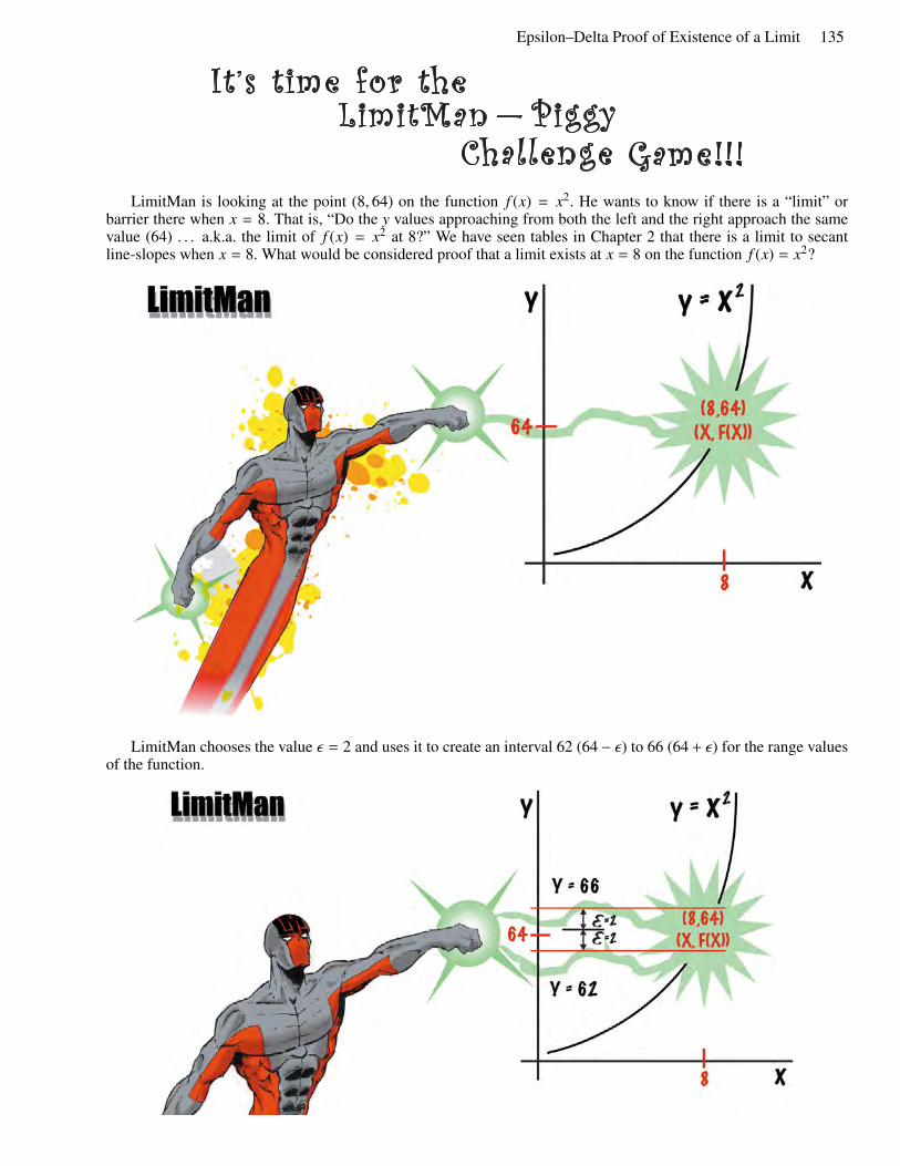
LimitMan is looking at the point (8, 64) on the function f (x) = x2. He wants to know if there is a “limit” orbarrier there when x = 8. That is, “Do the y values approaching from both the left and the right approach the samevalue (64) . . . a.k.a. the limit of f (x) = x2 at 8?” We have seen tables in Chapter 2 that there is a limit to secantline-slopes when x = 8. What would be considered proof that a limit exists at x = 8 on the function f (x) = x2?

LimitMan chooses the value � = 2 and uses it to create an interval 62 (64 − �) to 66 (64 + �) for the range valuesof the function.

Twenty Key Ideas in Beginning Calculus was conceived when the author noticed that many high school AP programs, especially English, often required summer reading for their students. Some math programs have been known to experiment with requiring the reading of historical books about mathematics or famous mathematicians, but they do not get much curricular payback for their students’ time. Meaningful, acces-sible, materials that could be assigned to students for summer reading and that would support the calcu-lus curriculum simply do not exist. Such materials sound like an oxymoron. Common wisdom has it that calculus materials are inherently too diffi cult for students to read and study on their own. Any attempt to create such materials would fail.

Twenty Key Ideas in Beginning Calculus does not claim or intend to be a calculus text. It is a creative sequencing and presentation of a subset of topics in the standard calculus curriculum. The author makes heavy use of “anticipatory sets,” “schedules of reinforcement,” “connection of mathematical ideas,” “con-nection to real-world applications,” pacing, patterns, visuals, examples and counterexamples, evolution and organization of ideas, repeated threading and spiraling of concepts, and especially repetition, repetition, and repetition. Four of the fourteen chapters (1, 2, 3, & 11) are written using only introductory algebra skills to introduce both calculus vocabulary and concepts. Limits and other major calculus concepts are taught intuitively using tables and visuals. All major proofs are relegated to the appendices, allowing stu-dents to customize their learning experience according to their ability and interest for rigor.

The author, Dan Umbarger, has taught various levels of mathematics from grade 5 to grade 12 for over 30 years. He currently teaches AP Computer Science at a Dallas area “majority minority” school. He is married and the proud father of three children: Jimmy, Terri, and Keelan. He is also the author of Explaining Logarithms and “Explaining Bayes Theorem” at www.mathlogarithms.com.

integral

deriv

ative

instantaneous-rate-of-speed

Division-by-Zero-ConnumdrumFundamental-theorum-of-Calculusproofs

relat

ed-r

ate-

prob

lems

decr

easin

g-ra

e-of

-spe

edm

ax-m

in-pr

oblem

s

deriv

ative

-of-

a-qu

otian

t Episilon-DeltaPower-Rule

Newton

The-Chain-RuleDe

finiti

on-o

f-f

Defin

ition

-of-

Area

-und

er-a

-Cur

ve derivative-of-difference

limitLeibnezgeneric-problem-sets

deriv

ative

-of-

sum

succesive-approximations

Proofsde

rivat

ive-o

f-pr

oduc

t

incre

asing

-rat

e-of

-spe

ed

slope

-of-

a-ta

ngen

t

preconditions for limits in beginning 18 calculus 6 · calculus, ftc 16 parallel theorems in...

Documents