SANDIA REPORTSAND2002-2398Unlimited ReleasePrinted July 2002

PREDICT User's Manual

Larry W. Young and Beverly R. Sturgis

Prepared bySandia National LaboratoriesAlbuquerque, New Mexico 87185 and Livermore, California 94550

Sandia is a multiprogram laboratory operated by Sandia Corporation,a Lockheed Martin Company, for the United States Department ofEnergy under Contract DE-AC04-94AL85000.

Approved for public release; further dissemination unlimited.

Issued by Sandia National Laboratories, operated for the United States Departmentof Energy by Sandia Corporation.

NOTICE: This report was prepared as an account of work sponsored by an agencyof the United States Government. Neither the United States Government, nor anyagency thereof, nor any of their employees, nor any of their contractors,subcontractors, or their employees, make any warranty, express or implied, orassume any legal liability or responsibility for the accuracy, completeness, orusefulness of any information, apparatus, product, or process disclosed, or representthat its use would not infringe privately owned rights. Reference herein to anyspecific commercial product, process, or service by trade name, trademark,manufacturer, or otherwise, does not necessarily constitute or imply its endorsement,recommendation, or favoring by the United States Government, any agency thereof,or any of their contractors or subcontractors. The views and opinions expressedherein do not necessarily state or reflect those of the United States Government, anyagency thereof, or any of their contractors.

Printed in the United States of America. This report has been reproduced directlyfrom the best available copy.

Available to DOE and DOE contractors fromU.S. Department of EnergyOffice of Scientific and Technical InformationP.O. Box 62Oak Ridge, TN 37831

Telephone: (865)576-8401Facsimile: (865)576-5728E-Mail: reports@adonis.osti.govOnline ordering: http://www.doe.gov/bridge

Available to the public fromU.S. Department of CommerceNational Technical Information Service5285 Port Royal RdSpringfield, VA 22161

Telephone: (800)553-6847Facsimile: (703)605-6900E-Mail: orders@ntis.fedworld.govOnline order: http://www.ntis.gov/ordering.htm

SAND2002-2398 Unlimited Release Printed July 2002

PREDICT User’s Manual

Larry W. Young

Mechanical and Structural Engineering Department

Beverly R. Sturgis

Applied Engineering and Technology Development Department

Sandia National Laboratories

P. O. Box 5800 Albuquerque, New Mexico 87185-0933

Abstract Sandia National Laboratories has developed a Near Real Time Range Safety Analysis Tool named PREDICT that is based upon a probabilistic range safety analysis process. Probabilistic calculations of risk may be used in place of the total containment of potentially hazardous debris during a missile launch operation. Impact probabilities are computed based upon probabilistic density functions, Monte Carlo trajectories of dispersion events, and missile failure scenarios. Impact probabilities are then coupled with current demographics (land populations, commercial and military ship traffic, and aircraft traffic) to produce expected casualty predictions for a particular launch window. Historically, these calculations required days of computer time to finalize. Sandia has developed a process that utilizes the IBM SP machines at the Maui High Performance Computing Center and at the Arctic Region Supercomputing Center to reduce the computation time from days to as little as an hour or two. This analysis tool then allows the Missile Flight Safety Officer to make launch decisions based on the latest information (winds, ship, and aircraft movements) utilizing an intelligent risk management approach. This report provides a user’s manual for PREDICT version 3.3. The work described in this report was performed for the Pacific Missile Range Facility under project number 1539 / tasks 1, 2, 3 and 4.

2

Acknowledgments

The process to produce probabilistic range safety analysis has been developed over a number of years with the contributions of several people. Robert LaFarge, Kenneth Cole, David Outka, William Millard, and Floyd Spencer all developed early programs used to produce breakup fragment definitions, impact propagations, and impact probability calculations. Terry Jordan-Culler, Larry Rollstin, Walter Rutledge, Walter Wolfe, William Millard, and John Morris (Naval Air Warfare Center) have all helped define the information required to make PREDICT a tool that is used during missile launch operations. A large thanks goes to David Salguero, author of the TAOS software, which was used as the basis for the propagation section of PREDICT. An additional thanks goes to Terry Jordan-Culler for reviewing and improving this document.

3

Contents

1 Introduction ................................................................................................................6

2 Impact Location Generation.............................................................................8

2.1 Breakup State Vectors .........................................................................................10 2.2 Breakup Models ....................................................................................................12 2.3 Wind Models .........................................................................................................12 2.4 Covariance Models...............................................................................................12

3 Probability of Impact Computations.........................................................13

4 Risk to Aircraft Computations......................................................................16

5 Output Data Analysis ..........................................................................................17

6 PREDICT Execution ...........................................................................................17

6.1 KIDD Intercept Runs...........................................................................................17 6.2 High-Performance Computing Centers...........................................................18 6.3 Maui High Performance Computing Center..................................................18 6.4 Arctic Region Supercomputing Center ...........................................................19

7 Problem Files ............................................................................................................19

7.1 File Format .............................................................................................................19 7.1.1 Data Blocks.....................................................................................................20 7.1.2 Names and Values...........................................................................................20 7.1.3 Comments .......................................................................................................20

7.2 *Title Data Block..................................................................................................20 7.3 *Propagate Data Block........................................................................................21

7.3.1 *Atmos Data Block.........................................................................................22 7.3.1.1 Standard Atmospheres ........................................................................22 7.3.1.2 RCC Atmospheres ..............................................................................24 7.3.1.3 Sonde-Measured Atmospheres ...........................................................25

7.3.2 *Montecarlo Data Block .................................................................................26 7.3.3 *Wind Data Block...........................................................................................27

7.3.3.1 Wind Table Format .............................................................................27 7.3.4 *Covariance Data Block .................................................................................28 7.3.5 *Stops Data Block...........................................................................................30 7.3.6 *Breakup Data Block......................................................................................30

4

7.3.6.1 *Model Data Block .............................................................................30 7.3.6.1.1 *Piece Data Block ..............................................................31

7.3.6.2 *Statevectors Data Block....................................................................32 7.3.6.3 *Roll Data Block.................................................................................33

7.3.7 *Intercept Data Block .....................................................................................34 7.3.7.1 *FASTT Data Block ...........................................................................34 7.3.7.2 *KIDD Data Block .............................................................................34

7.4 *PDF Data Block..................................................................................................37 7.4.1 *Files Data Block............................................................................................37 7.4.2 *Options Data Block.......................................................................................38 7.4.3 *Include Data Block .......................................................................................40 7.4.4 *Contours Data Block.....................................................................................40 7.4.5 *Plot Data Block .............................................................................................40 7.4.6 *Minke Data Block .........................................................................................40 7.4.7 *Minmv Data Block........................................................................................40 7.4.8 *Time Data Block ...........................................................................................41 7.4.9 *Popcenter Data Block ...................................................................................41

7.5 *Tools Data Block................................................................................................42 7.5.1 *Popcenter Data Block ...................................................................................42 7.5.2 *Union Data Block .........................................................................................43 7.5.3 *Contours Data Block.....................................................................................44 7.5.4 *Path Data Block ............................................................................................45 7.5.5 *RRAT Data Block.........................................................................................47 7.5.6 *TECPLOT Data Block..................................................................................48 7.5.7 *Covariance Data Block .................................................................................48

7.6 *End Data Block...................................................................................................50

Figures

Figure 1-1. Generic Range Safety Analysis ........................................................................7 Figure 2-1. Internal Procedure to Initialize and Propagate Breakup Fragments .................9 Figure 2-2. Generation of Breakup State Vectors .............................................................11 Figure 4-1. Example of Aircraft Probability of Impact vs. Time ......................................16 Figure 7-1. Equal Probability Segments of Normal Distribution ......................................26 Figure 7-2. Defining a Computational Box .......................................................................39

Tables

Table 3-1. Defining Parameters for the Impact Probability Density Functions .....................14 Table 3-2. Bivariate Gaussian Density Function ....................................................................14 Table 3-3. Impact Density Function for an Arbitrary Longitude and Latitude ......................15 Table 7-1. Standard Atmosphere Models ...............................................................................23 Table 7-2. RCC Atmosphere Types........................................................................................24

5

Nomenclature

3 DOF 3 Degrees Of Freedom (point mass)

6 DOF 6 Degrees Of Freedom

ARSC Arctic Region Supercomputing Center

Ec Expected casualties

ECFC Earth-Centered and Fixed Cartesian coordinate system (axis 1 through Greenwich meridian; axis 3 through North Pole)

ECI Earth-Centered Inertial Cartesian coordinate system (ECFC frame frozen at some instant in time)

FTS Flight Termination System

IIP Instantaneous Impact Point

KTF Kauai Test Facility

LHS Latin Hypercube Sampling

MHPCC Maui High Performance Computing Center

PDF Probability Density Function

PI Probability of Impact

RCC Range Commander’s Council

Body 3-2-1 rotation A rotation sequence to orient frame B with respect to frame A:

I) align frames A and B so axis 1 of A aligns with axis 1 of B, etc.

II) rotate B about axis 3 of B to arrive at frame B’

III) rotate B’ about axis 2 of B’ to arrive at frame B’’

IV) rotate B’’ about axis 1 of B’’ to arrive at frame B

Breakup time Time the missile destructs

Failure mode Type of failure (e.g., stuck nozzle)

Failure time Time a failure (e.g., stuck nozzle) occurs

Failure trajectory Trajectory flown after a failure occurs

Fragment class Type of fragment (e.g., bolt)

Intact breakup model Breakup model for nominal flight (e.g. spent 1st stage, etc.)

Local geodetic frame North, east, down coordinate system at current position

6

1 Introduction

To produce a probabilistic range safety analysis for a missile launch or a missile intercept requires a vast amount of time and resources. In the past, several stand-alone computer programs were used to perform a range safety analysis. It was not uncommon to take several weeks using multiple individual central processing units to produce a set of probability impact data once all of the input data were available. PREDICT� was developed to reduce the time required to produce results so that day-of-launch decisions could be based upon the latest possible data. The PREDICT computer program combines the stand-alone programs used previously into a faster, more user-friendly program with the added capability described in this report. To further enhance the computation speed it is possible to execute this program in a parallel computing environment.

The set of input data requirements is application dependent. The user must supply some or all of the following information: the missile system breakup model(s), the wind model, the off-nominal covariance matrices at various destruct times, the state vectors at destruct or intercept, and the probability of failure associated with each failure scenario. For an intercept of two bodies colliding, a fragmentation code is called by PREDICT to provide the breakup model and an initial state vector for each fragment.

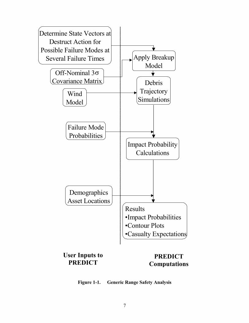
The procedure to produce a range safety analysis may be divided into four parts. Part 1 is the computation of the impact locations for all fragments in the breakup model. For a missile destruct case, the breakup is assumed to occur at many possible combinations of breakup times and failure modes. For the intercept case, the breakup is assumed to occur at a known location and intercept geometry. Part 2 takes all of the impact location information computed during Part 1 and combines these locations with the failure probability of each failure trajectory to produce probability of impact data over a user-specified latitude, longitude grid. Part 3 defines the aircraft safety study requirements. Part 4 provides data analysis capabilities. These parts are discussed in sections 2 through 5 below. Figure 1-1 shows a generic range safety analysis flowchart. PREDICT is a non-interactive computer program. All input data reside in one or more files created prior to running PREDICT. As PREDICT runs, it creates one or more output files. These output files cannot be used until PREDICT has completed execution. Each of the input and output files are text files that can be created, inspected and modified with any text editor or word processor.

PREDICT uses a problem file to define all program input information. The problem file uses a data block format as described in Section 7. The data blocks include all the instructions and file names necessary for PREDICT to execute the user-defined problem.

� PREDICT is not an acronym; rather, it was chosen to describe how the flight safety analysis “predicts” the probable risk to people and assets.

7

Off-Nominal 3 �

Covariance Matrix

Determine State Vectors at Destruct Action for

Possible Failure Modes at Several Failure Times Apply Breakup

Model

Debris

Trajectory Simulations

Impact Probability

Calculations

Results • Impact Probabilities • Contour Plots

• Casualty Expectations

Failure Mode Probabilities

Demographics

Asset Locations

Wind

Model

Figure 1-1. Generic Range Safety Analysis

User Inputs toPREDICT

PREDICT Computations

8

2 Impact Location Generation

A flying missile may be destroyed because of the following causes: (1) an inadvertent flight termination system (FTS) action is taken while the missile is flying a near nominal trajectory, (2) a failure causes the missile to fly off course and an FTS signal is sent to destroy it, (3) the missile self destructs because of structural breakup, or (4) the missile impacts a target vehicle. In each of these cases, fragments are created at the breakup location. Information about each of the fragments is generated from the missile’s state vector at the time of breakup and from the breakup model for the missile configuration at the time of breakup. These data provide initial conditions for each fragment (e.g., position, velocity, ballistic coefficient). PREDICT alters the initial conditions by applying covariance information to the position and velocity components of the breakup state vector. In addition, the user may choose to apply statistics to the fragment’s ballistic coefficient, velocity increment due to the destruct action and the wind profile through which the fragment will fly.

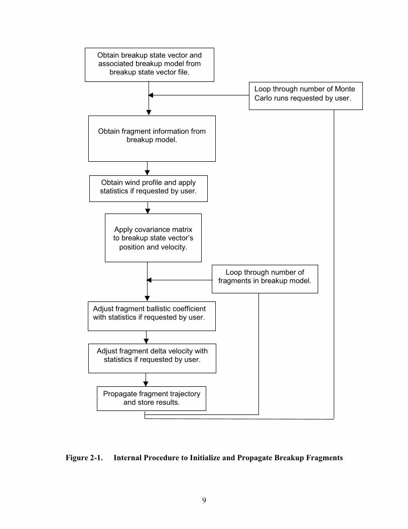
Once the fragment’s initial conditions have been computed and any user-specified statistics have been applied, the three degree of freedom (3 DOF) propagator in PREDICT propagates each fragment’s instantaneous impact point (IIP) from breakup to all altitudes specified by the user. The PREDICT propagator uses essentially the same methods employed by TAOS.1 (Modifications were made to the TAOS propagator to handle the multiple impact altitudes required for the aircraft safety studies.) The resulting ballistic trajectory has no propulsive forces and employs a user-supplied drag coefficient or ballistic coefficient model for aerodynamics. This initialization and propagation process is performed multiple times for each fragment to provide a Monte Carlo set of trajectories for each fragment. Figure 2-1 summarizes this process for a non-intercept scenario.

Each of the input files that the user must provide to PREDICT to compute impact locations at desired altitudes is discussed in the following sections. Various altitudes are sometimes desired in order to determine risk to aircraft as well as risk to people and assets on the ground.

9

Figure 2-1. Internal Procedure to Initialize and Propagate Breakup Fragments

Obtain breakup state vector and associated breakup model from

breakup state vector file.

Loop through number of Monte Carlo runs requested by user.

Obtain wind profile and apply statistics if requested by user.

Obtain fragment information from

breakup model.

Apply covariance matrix to breakup state vector’s

position and velocity.

Adjust fragment ballistic coefficient with statistics if requested by user.

Adjust fragment delta velocity with statistics if requested by user.

Loop through number of fragments in breakup model.

Propagate fragment trajectory and store results.

10

2.1 Breakup State Vectors

For a missile destruct action, the user must supply a breakup state vector file to PREDICT. This file contains position, velocity, and attitude information about the missile at the time an FTS action or structural failure occurs. For inclusion of the nominal trajectory without a destruct action, this information reflects the missile’s state vector at the end of powered flight. State vector information includes the breakup time and the missile’s position (altitude, latitude, longitude), velocity with respect to an earth fixed observer (velocity magnitude, horizontal and vertical flight path angles), and attitude (body 3-2-1 yaw, pitch, roll angles between the body fixed frame and the local geodetic frame). Other information recorded in this file includes the failure mode, the probability of the failure mode occurring, the failure time, the breakup time, and the breakup model to be used for the breakup state vector. An example of a breakup state vector file is given in Section 7.3.6.2. Failure modes are either destruct actions along the nominal flight path (inadvertent FTS actions) or system failures that cause the missile to fly off course. Examples of system failures are stuck nozzles, a computer failure, or a guidance system failure. Since impacts from a nominal trajectory (e.g., impact of a spent first-stage motor) are also important, “nominal” events may also be included in a breakup state vector file even though they are not really failures. The failure time is the time a failure occurs. For an inadvertent FTS action, the failure time is the time the FTS action occurs. For a stuck nozzle, the failure time is the time the nozzle initially becomes stuck in place.

The breakup time is the time when the missile breaks into fragments. This time is greater than or equal to the failure time since the missile may fly for some time after a failure occurs but before it is destroyed. For example, a nozzle might become stuck in place several seconds into a motor burn, but other nozzles attempt to correct the error and a destruct action may not result until later in the trajectory. A failure trajectory is the trajectory the missile flies after a failure occurs. Since there are many possible failure modes and failure times, there will be many failure trajectories for the missile. (These trajectories are generated before PREDICT is executed.) They are typically six degree of freedom (6 DOF) trajectories and are flown using software that includes representative guidance and control algorithms. For each failure trajectory, the missile is flown along its nominal path until the failure time for that trajectory is reached. At that time, the failure mode for that trajectory is activated (e.g., a nozzle becomes stuck) and the resulting trajectory is calculated. Once the set of failure trajectories is obtained, the set is checked for violations of the destruct criteria (IIP limit, angle of attack limit, etc.). If a failure trajectory violates any of the destruct criteria, the FTS is activated and the missile state at breakup is recorded to the breakup state vector file. If no destruct criteria

11

are violated, the breakup state vector recorded to the breakup state vector file is the state vector at the end of powered flight. This process is summarized in Figure 2-2. The entire process described in this section is performed before PREDICT is executed. If a missile strikes a target vehicle (an intercept case), the breakup state vector file is not needed. Instead a debris generation code (KIDD2 or FASTT3) is called by PREDICT to provide initial fragment state vector information.

Figure 2-2. Generation of Breakup State Vectors

Missile flies a nominal path until failure time is reached (e.g., nozzle sticks at

failure time)

Failure mode (e.g., stuck nozzle) is activated and trajectory continues

along altered path

Destruct criteria violated? (e.g., IIP limit, angle of attack limit, etc.)

yesno

FTS action results; breakup state vector is state vector at time of FTS action; appropriate breakup model is chosen

No FTS action results; breakup state vector is state

vector at end of powered flight; intact breakup model is

chosen

Breakup state vector info and breakup model name are written to state vector file for use in

PREDICT

12

2.2 Breakup Models

The breakup model tells PREDICT which fragments are created when the missile is destroyed and gives information about each of those fragments. Two cases exist that require different methods for supplying vehicle breakup information. One case is an intercept scenario in which two impacting bodies break into fragments because of their collision. In this case, the user does not provide breakup models. Instead the *intercept data block is used, and either the KIDD2 or FASTT3 breakup model is called from PREDICT to generate the debris from the collision. The user tells PREDICT which debris-generation code to call by using either the *FASTT or the *KIDD data block after the *intercept data block. The other case is a breakup scenario in which the missile is destroyed because of structural breakup or an FTS action. This type of scenario is specified by using the *breakup data block. In these situations, the user must determine the fragments produced when the missile is destroyed. For each fragment, the weight, ballistic coefficient, any velocity increment and direction that may exist because of the destruct action, and any change in the fragment’s mass over time are defined. Since many missile configurations may change during the course of flight, it is likely that more than one breakup model will be defined. For example, the missile configuration during first stage burn differs from that during third stage burn, and the fragments resulting from a breakup during these two segments of flight will differ from one other.

More discussion and examples of user-defined breakup models are given in Section 7.3.6. Section 7.3.7 provides an example for an intercept case.

2.3 Wind Models

Atmospheric winds with respect to the earth’s surface are defined with a *wind data block. If a *wind data block is not input, all wind velocities are set to zero. Winds defined in a *wind data block apply to the entire *problem block in which the *wind data block is defined. By default, wind components are aligned with the local geodetic coordinate system. The wind is only a function of altitude and has no vertical or downward components. The east wind component is positive when the wind is from the east (moving from east to west), and the north component is positive when the wind is from the north (moving from north to south). If statistics are to be applied to the wind, the user sets parameters in the *wind data block to accomplish this action. Section 7.3.3 provides examples and further discussion.

2.4 Covariance Models

PREDICT alters a fragment’s initial conditions by applying a covariance matrix to the state vector obtained from the breakup state vector file. The covariance matrix is a 6x6 matrix containing the covariance values in position and velocity. The user must supply this covariance matrix as a function of time. PREDICT is able to generate the covariance

13

matrix for the user in a separate run if so desired. In this case the user supplies nominal and off-nominal trajectories to PREDICT. If a nominal trajectory is not provided, PREDICT computes an average trajectory from the off-nominal trajectories and uses it in place of a nominal trajectory in the formation of the covariance values. An example of a covariance file is provided in Section 7.3.4. Section 7.5.7 describes the process that PREDICT uses to compute the covariance matrix in a separate run.

3 Probability of Impact Computations

Computation of the probability of impact contour plots requires the impact locations generated previously and the probability of failure associated with each failure trajectory. The impact probability data are computed over a user-specified latitude, longitude grid. PREDICT may be run with one single problem file that generates the impact locations and the probability of impact files, or it may be run with two or more sequential problem files where impact locations are computed in the first run and stored as output files. These files become inputs for subsequent problem files to compute impact probabilities. The impact data generated from Monte Carlo techniques can be used to develop a statistical model of the impact likelihood for an area on the earth's surface. The statistical model is constructed from subsets of the impact data, where each subset consists of all the impacts resulting from a given combination of the systematically varied impact mode parameters. For impacts resulting from failures (non-intercept cases), the systematically varied impact mode parameters are the failure time, the fragment class, and the failure mode.

The impact points vary because of the random variations in some flight parameters (e.g., breakup time state vectors, imparted fragment velocities and directions, and the wind profile). Since two or more of these variations are Gaussian in nature, it can be expected that for each such subset, the impact point variations will also approximate a Gaussian distribution. Hence, for each such subset, five parameters describing the corresponding Gaussian impact point distribution function are computed: mean longitude and latitude, standard deviations in longitude and latitude, and the correlation coefficient relating deviations from the mean in longitude with those in latitude.

The equations for defining parameters for the impact probability density functions (PDFs) are given in Table 3-1. Here, �i is the ith impact longitude of the subset, �i is the ith impact latitude of the subset, and n is the number of impact points in the subset.

14

Table 3-1. Defining Parameters for the Impact Probability Density Functions

The value of the PDF function at an arbitrary longitude, �, and latitude, �, is given by the bivariate Gaussian density function as shown in Table 3-2. This function is an exponential function of the five defining parameters given in Table 3-1.

Table 3-2. Bivariate Gaussian Density Function

To obtain the impact probability density functions for all combinations of the time of failure, fragment class and type of failure, the subset of PDFs is combined numerically in the following manner.

First a grid of latitude, longitude points in the area of interest is defined. The number of impacts per unit area is computed at each of the grid points. For each grid point and

Mean longitude �

�

�

n

iin 1

1��

Mean latitude �

�

�

n

iin 1

1��

Standard deviation of longitude

� ���

�

�

�

n

iin 1

2

11

����

Standard deviation of latitude � ��

�

�

�

�

n

iin 1

2

11

����

Correlation coefficient

� �� �� �

� � � ���

�

��

�

��

��

�

n

ii

n

ii

n

iii

1

2

1

2

1

����

����

���

� �� �

� � � �� � � �

2

212

1

12,

2

2

2

2

2

����

�

��

��

�����

�

��

�

������

���

��

���

�

�

��

���

��

���

��

��

�

��

���

�

�

�

epdf

15

combination of failure mode and fragment class, the density of impacts expected for all times is obtained.

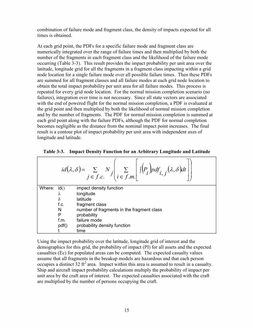
At each grid point, the PDFs for a specific failure mode and fragment class are numerically integrated over the range of failure times and then multiplied by both the number of the fragments in each fragment class and the likelihood of the failure mode occurring (Table 3-3). This result provides the impact probability per unit area over the latitude, longitude grid for all the fragments in a fragment class impacting within a grid node location for a single failure mode over all possible failure times. Then these PDFs are summed for all fragment classes and all failure modes at each grid node location to obtain the total impact probability per unit area for all failure modes. This process is repeated for every grid node location. For the normal mission completion scenario (no failures), integration over time is not necessary. Since all state vectors are associated with the end of powered flight for the normal mission completion, a PDF is evaluated at the grid point and then multiplied by both the likelihood of normal mission completion and by the number of fragments. The PDF for normal mission completion is summed at each grid point along with the failure PDFs, although the PDF for normal completion becomes negligible as the distance from the nominal impact point increases. The final result is a contour plot of impact probability per unit area with independent axes of longitude and latitude.

Table 3-3. Impact Density Function for an Arbitrary Longitude and Latitude

� � � � � ��� �

��

�

�

���

�

�

��

�

��

�

��.. ..

,,,cfj mfi

dtjipdfiPjNid ����

Where: id() impact density function �� longitude �� latitude f.c. fragment class N number of fragments in the fragment class P probability f.m. failure mode pdf() probability density function t time

Using the impact probability over the latitude, longitude grid of interest and the demographics for this grid, the probability of impact (PI) for all assets and the expected casualties (Ec) for populated areas can be computed. The expected casualty values assume that all fragments in the breakup models are hazardous and that each person occupies a distinct 32 ft2 area. Impact within this area is assumed to result in a casualty. Ship and aircraft impact probability calculations multiply the probability of impact per unit area by the craft area of interest. The expected casualties associated with the craft are multiplied by the number of persons occupying the craft.

16

4 Risk to Aircraft Computations

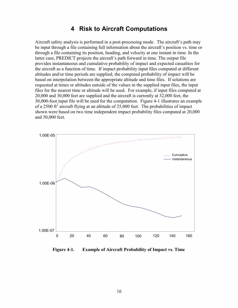
Aircraft safety analysis is performed in a post-processing mode. The aircraft’s path may be input through a file containing full information about the aircraft’s position vs. time or through a file containing its position, heading, and velocity at one instant in time. In the latter case, PREDICT projects the aircraft’s path forward in time. The output file provides instantaneous and cumulative probability of impact and expected casualties for the aircraft as a function of time. If impact probability input files computed at different altitudes and/or time periods are supplied, the computed probability of impact will be based on interpolation between the appropriate altitude and time files. If solutions are requested at times or altitudes outside of the values in the supplied input files, the input files for the nearest time or altitude will be used. For example, if input files computed at 20,000 and 30,000 feet are supplied and the aircraft is currently at 32,000 feet, the 30,000-foot input file will be used for the computation. Figure 4-1 illustrates an example of a 2500 ft2 aircraft flying at an altitude of 25,000 feet. The probabilities of impact shown were based on two time independent impact probability files computed at 20,000 and 30,000 feet.

Figure 4-1. Example of Aircraft Probability of Impact vs. Time

1.00E-07

1.00E-06

1.00E-05

0 20 40 60 80 100 120 140 160

Cumulative Instantaneous

17

5 Output Data Analysis

The output data from PREDICT may be presented in several forms. A contour plot of the impact probabilities is the most commonly used presentation form. The capability exists to produce files to be used by display programs such as Tecplot�. Tabulation of impact probabilities for specific assets is another output format. Several tools are available to assist with data analysis. Each of these tools is discussed and examples are provided in Section 7.5.

6 PREDICT Execution

In general, the PREDICT computer program is executed by entering a command that consists of the PREDICT executable file name followed by command line options. The -p option defines the input problem file name and the –s option defines the output status file name. The status file is essentially a log of PREDICT’s actions. If no command line options are provided, PREDICT uses the default file names of PROBLEM for the problem file name and PRINT for the status file name. On many computers, an alias, link, or path may be set up so that the command PREDICT runs the appropriate file:

% PREDICT –p file.prb –s file.status

If an alias is not used, the full path and PREDICT executable name must be provided:

% /fullpath/predict.exe –p file.prb –s file.status

6.1 KIDD Intercept Runs

For operation on a UNIX or DOS operating system, an environment variable must be set to locate the KIDD2 program executable.

For a UNIX operating system the following command must be added to the user’s .cshrc file:

setenv KIDDEXE ‘full path to the KIDD executable’ (The single quotes around the path + executable name must be included.)

For a Windows environment, the following steps are required:

Windows98 Start � Settings � Control Panel Double click on System icon Select the Environment tab

18

Create a new variable named KIDDEXE with a value that is the path to the KIDD executable

Windows2000 Start � Settings � Control Panel Double click on System icon Select Advanced Select the Environment Variables option Create a new user variable named KIDDEXE with a value that is the path to the

KIDD executable

6.2 High-Performance Computing Centers

PREDICT is available for execution on the IBM SP parallel computers located at the Maui High Performance Computing Center (MHPCC) and at the Arctic Region Supercomputing Center (ARSC). The breakup, propagation, and impact probability computations have been set up in a pseudo-parallel manner such that they run on separate processors. This significantly reduces run time. Users of these computing centers must have an established account with adequate disk space for output files, or they must operate from one of the scratch disk spaces. The computing center must be contacted to establish a user account and to obtain current login procedures.

6.3 Maui High Performance Computing Center

At the time of this writing, the IBM SP machine used at MHPCC is called “tempest.” PREDICT is run on this machine with an interactive pre-processing program named maui_all.C. An alias name is recommended to make the program easy to use. For example, if using the c-shell, the line

alias PREDICT /u/brsturg/maui_all.exe

can be added to the .cshrc file in the user’s home directory to define an alias called PREDICT that points to the pre-processing program.

The pre-processing program begins by displaying a main menu, for example,

% PREDICT PREDICT (Version x.x)

0 – Exit 1 – Submit Job 2 – Check Job Queue

>

Option 1 will prompt for the problem file name, the status file name, the number of processors needed, an account number, a time limit, and an e-mail address to use for notification. A separate job must be submitted for each problem file. The pre-processing program then automatically submits the job to the IBM SP computer.

19

Option 2 displays the status of the jobs that have been submitted. After submitting a job, it generally takes about a minute before it shows up in the queue. When the job disappears from the queue, it has finished. An e-mail message will be sent as a notification that the job has finished.

PREDICT creates output files on the root processor that are automatically copied to the user’s directory. A status file is created on each processor. Each status file has a number attached to it corresponding to the processor that created it. The pre-processing program automatically deletes the files on each processor once these files have been copied back to the user’s directory.

6.4 Arctic Region Supercomputing Center

At the time of publication, the IBM SP machine used at ARSC is called “icehawk.” The job submission procedure at ARSC is identical to that at MHPCC except that the interactive pre-processing program is named arsc_all.C.

7 Problem Files

7.1 File Format

Problem files contain the information required to compute a set of impact locations and/or the impact probability data resulting from those impact locations. A problem file may contain one or more problems. Problem files are text files so they can be created with any standard text editor such as UNIX’s vi or Windows Wordpad. They may also be created with other software such as an interactive design code.

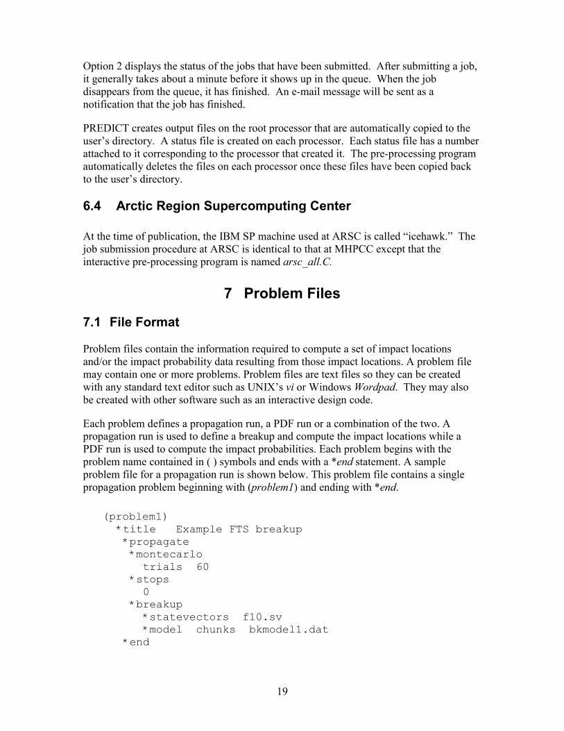
Each problem defines a propagation run, a PDF run or a combination of the two. A propagation run is used to define a breakup and compute the impact locations while a PDF run is used to compute the impact probabilities. Each problem begins with the problem name contained in ( ) symbols and ends with a *end statement. A sample problem file for a propagation run is shown below. This problem file contains a single propagation problem beginning with (problem1) and ending with *end.

(problem1) *title Example FTS breakup *propagate *montecarlo trials 60 *stops 0 *breakup *statevectors f10.sv *model chunks bkmodel1.dat *end

20

7.1.1 Data Blocks

Each set of information, or data block, in the problem file begins with an asterisk and a name, for example, *title, *montecarlo, *model. These are special PREDICT keywords that identify the type of information that follows.

Information from problem files is read into PREDICT one line at a time. Each line of text contains some names and values separated by special characters such as spaces or commas. These special characters are called delimiters. Valid delimiters are white-space characters (space, tab, etc.), commas, equal signs, parentheses, colons, greater-than signs, and less-than signs. Because delimiters are used to separate names and values, they cannot be embedded within a name or value.

Internally, PREDICT requires names that are lowercase. Names and keywords entered in uppercase are automatically converted to lowercase, so case is not important from a user’s standpoint.

7.1.2 Names and Values

Names and values can be placed anywhere on a line. They do not have to be in certain columns. This free-field style of input allows indentation to make it easier to visualize the problem file structure and to avoid input errors.

Numerical values can be input as integers without a decimal point, as real numbers with a decimal point or as real numbers in scientific notation (e-format).

Note that delimiters cannot be embedded within a value, so the value

wgt = 10,000 # Incorrect value

is incorrect. The comma is interpreted as a delimiter, so PREDICT thinks there are two values instead of one. In this case, it reads 10 and 0 instead of 10000.

7.1.3 Comments

Comments, starting with the special character #, can be placed anywhere in a problem file. Comments extend from the # character to the end of the line. Blank lines are ignored, so they can be used to put space between sections of information for easier reading.

7.2 *Title Data Block

A problem title, consisting of one or more lines of text, is optional.

21

A title can be used to help identify or document a problem. There is no limit on the number of lines in a title.

*title This is the first line of the title and this is the second line of the title

and so on, until the next data block name occurs.

*wind

The title begins with the first nonblank character following the *title keyword and extends to the next valid data block keyword. In the example above, the title extends from the word This to just before the *wind keyword; thus, a title may contain any text except for data block keywords. All data block keywords begin with an asterisk, so difficulties can be avoided by not putting asterisks in front of a word in the title.

7.3 *Propagate Data Block

The *propagate data block is used to define the breakup model(s), the off-nominal covariance matrices and the file names and desired altitudes for the computed impact data. The allowable data blocks following *propagate are *atmos, *montecarlo, *wind, *covariance, *stops, *breakup and *intercept. Resulting impact data files will be created by PREDICT with the file names automatically generated. The file names for a *breakup data block will be of the form BK_(breakup_model_name)-FT_(failure time)-ALT_(impact_altitude).pdf. The failure time will be rounded to the nearest whole second. To prevent overwriting of files, the pdf extension will be incremented (.pdf1) for a maximum of six files (filename.pdf, filename.pdf1, filename.pdf2, filename.pdf3, filename.pdf4, filename.pdf5).

For example, suppose a breakup state vector file contains state vectors for failure times of 2 seconds and 4 seconds and each of these failures uses a breakup model called “stage1.” In addition, the user has requested impact altitudes of 0 and 10000 feet. PREDICT will then create impact data files named BK_stage1-FT_2-ALT_0.pdf, BK_stage1-FT_4-ALT_0.pdf, BK_stage1-FT_2-ALT_10000.pdf, and BK_stage1-FT_4-ALT_10000.pdf. If a file called BK_stage1-FT_2-ALT_0.pdf already exists, then PREDICT will not overwrite that file but will create a file called BK_stage1-FT_2-ALT_0.pdf1. The same procedure is used for naming impact data files when either the *FASTT or *KIDD data blocks are used instead of a user-defined breakup model. The only difference is that the file name begins with “FASTT” or “KIDD” rather than “BK.”

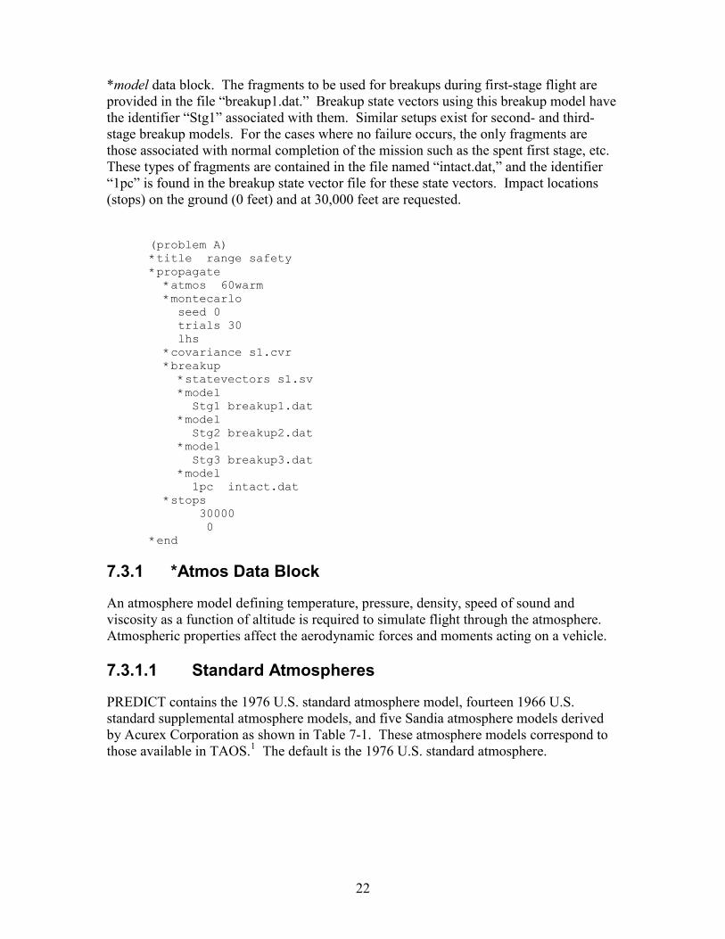
An example of a problem file for a propagation run using a user-supplied breakup model is given below. This problem file chooses the 60� latitude, warm season (60warm) atmosphere model. It specifies 30 Monte Carlo trajectories (trials) for each fragment of the breakup model and uses Latin Hypercube sampling (LHS) for the Monte Carlo process. The covariance matrix as a function of time is supplied in file s1.cvr while the breakup state vectors are located in file s1.sv. Four breakup models are supplied in the

22

*model data block. The fragments to be used for breakups during first-stage flight are provided in the file “breakup1.dat.” Breakup state vectors using this breakup model have the identifier “Stg1” associated with them. Similar setups exist for second- and third-stage breakup models. For the cases where no failure occurs, the only fragments are those associated with normal completion of the mission such as the spent first stage, etc. These types of fragments are contained in the file named “intact.dat,” and the identifier “1pc” is found in the breakup state vector file for these state vectors. Impact locations (stops) on the ground (0 feet) and at 30,000 feet are requested.

(problem A) *title range safety *propagate *atmos 60warm *montecarlo seed 0 trials 30 lhs *covariance s1.cvr *breakup *statevectors s1.sv *model Stg1 breakup1.dat *model Stg2 breakup2.dat *model Stg3 breakup3.dat *model 1pc intact.dat *stops 30000 0 *end

7.3.1 *Atmos Data Block

An atmosphere model defining temperature, pressure, density, speed of sound and viscosity as a function of altitude is required to simulate flight through the atmosphere. Atmospheric properties affect the aerodynamic forces and moments acting on a vehicle.

7.3.1.1 Standard Atmospheres

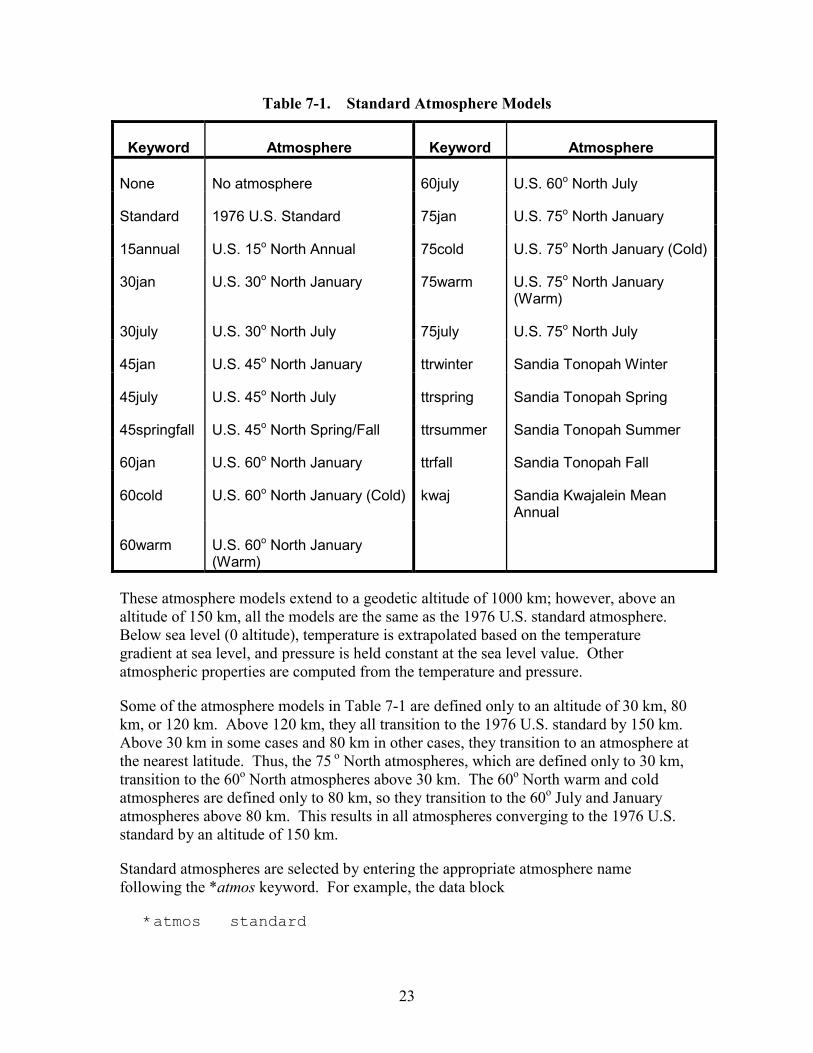
PREDICT contains the 1976 U.S. standard atmosphere model, fourteen 1966 U.S. standard supplemental atmosphere models, and five Sandia atmosphere models derived by Acurex Corporation as shown in Table 7-1. These atmosphere models correspond to those available in TAOS.1 The default is the 1976 U.S. standard atmosphere.

23

Table 7-1. Standard Atmosphere Models

Keyword Atmosphere Keyword Atmosphere

None No atmosphere 60july U.S. 60o North July

Standard 1976 U.S. Standard 75jan U.S. 75o North January

15annual U.S. 15o North Annual 75cold U.S. 75o North January (Cold)

30jan U.S. 30o North January 75warm U.S. 75o North January (Warm)

30july U.S. 30o North July 75july U.S. 75o North July

45jan U.S. 45o North January ttrwinter Sandia Tonopah Winter

45july U.S. 45o North July ttrspring Sandia Tonopah Spring

45springfall U.S. 45o North Spring/Fall ttrsummer Sandia Tonopah Summer

60jan U.S. 60o North January ttrfall Sandia Tonopah Fall

60cold U.S. 60o North January (Cold) kwaj Sandia Kwajalein Mean Annual

60warm U.S. 60o North January (Warm)

These atmosphere models extend to a geodetic altitude of 1000 km; however, above an altitude of 150 km, all the models are the same as the 1976 U.S. standard atmosphere. Below sea level (0 altitude), temperature is extrapolated based on the temperature gradient at sea level, and pressure is held constant at the sea level value. Other atmospheric properties are computed from the temperature and pressure.

Some of the atmosphere models in Table 7-1 are defined only to an altitude of 30 km, 80 km, or 120 km. Above 120 km, they all transition to the 1976 U.S. standard by 150 km. Above 30 km in some cases and 80 km in other cases, they transition to an atmosphere at the nearest latitude. Thus, the 75 o North atmospheres, which are defined only to 30 km, transition to the 60o North atmospheres above 30 km. The 60o North warm and cold atmospheres are defined only to 80 km, so they transition to the 60o July and January atmospheres above 80 km. This results in all atmospheres converging to the 1976 U.S. standard by an altitude of 150 km.

Standard atmospheres are selected by entering the appropriate atmosphere name following the *atmos keyword. For example, the data block

*atmos standard

24

selects the 1976 U.S. standard atmosphere model while the data block

*atmos ttrfall

selects the Tonopah Test Range (TTR) Fall atmosphere model. The selected atmosphere model applies to all computations within a *problem data block.

7.3.1.2 RCC Atmospheres

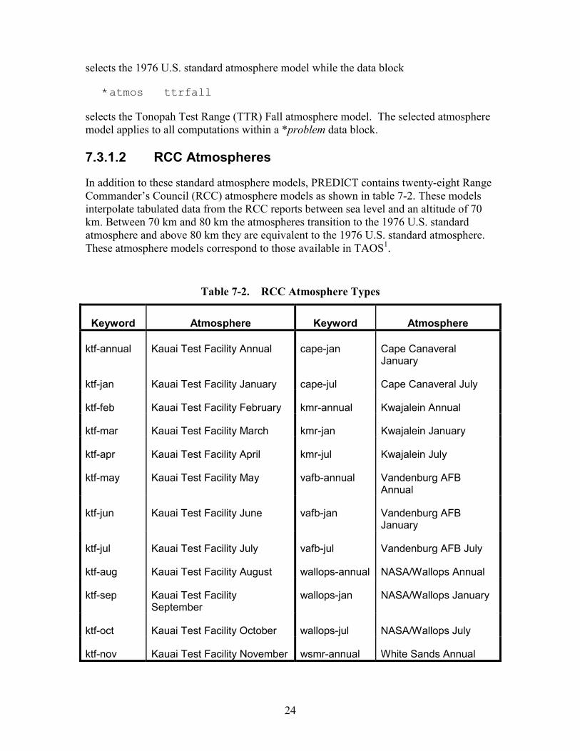
In addition to these standard atmosphere models, PREDICT contains twenty-eight Range Commander’s Council (RCC) atmosphere models as shown in table 7-2. These models interpolate tabulated data from the RCC reports between sea level and an altitude of 70 km. Between 70 km and 80 km the atmospheres transition to the 1976 U.S. standard atmosphere and above 80 km they are equivalent to the 1976 U.S. standard atmosphere. These atmosphere models correspond to those available in TAOS1.

Table 7-2. RCC Atmosphere Types

Keyword Atmosphere Keyword Atmosphere

ktf-annual Kauai Test Facility Annual cape-jan Cape Canaveral January

ktf-jan Kauai Test Facility January cape-jul Cape Canaveral July

ktf-feb Kauai Test Facility February kmr-annual Kwajalein Annual

ktf-mar Kauai Test Facility March kmr-jan Kwajalein January

ktf-apr Kauai Test Facility April kmr-jul Kwajalein July

ktf-may Kauai Test Facility May vafb-annual Vandenburg AFB Annual

ktf-jun Kauai Test Facility June vafb-jan Vandenburg AFB January

ktf-jul Kauai Test Facility July vafb-jul Vandenburg AFB July

ktf-aug Kauai Test Facility August wallops-annual NASA/Wallops Annual

ktf-sep Kauai Test Facility September

wallops-jan NASA/Wallops January

ktf-oct Kauai Test Facility October wallops-jul NASA/Wallops July

ktf-nov Kauai Test Facility November wsmr-annual White Sands Annual

25

ktf-dec Kauai Test Facility December wsmr-jan White Sands January

cape-annual

Cape Canaveral Annual wsmr-jul White Sands July

RCC atmospheres are selected with the keyword rcc following the *atmos keyword. The rcc keyword is followed by the RCC atmosphere type; for example, the data block

*atmos rcc ktf-dec

selects the Kauai Test Facility (KTF) December atmosphere from the Barking Sands, Kauai RCC 370-83 report.

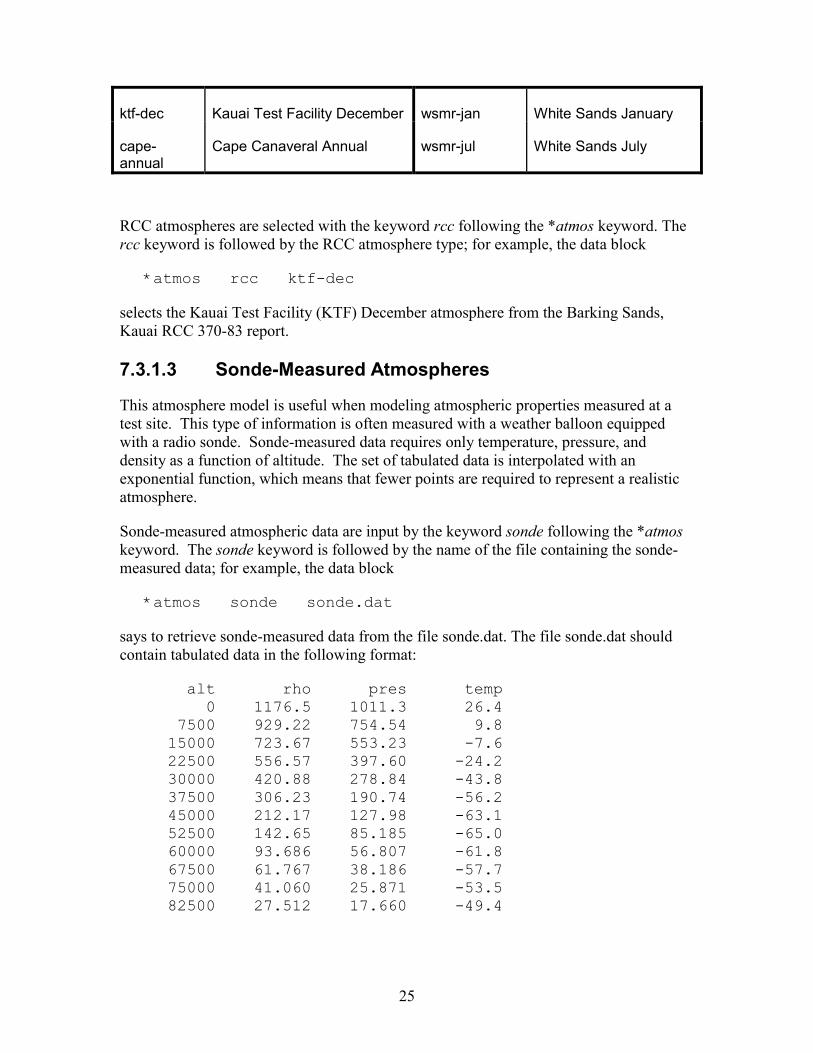
7.3.1.3 Sonde-Measured Atmospheres

This atmosphere model is useful when modeling atmospheric properties measured at a test site. This type of information is often measured with a weather balloon equipped with a radio sonde. Sonde-measured data requires only temperature, pressure, and density as a function of altitude. The set of tabulated data is interpolated with an exponential function, which means that fewer points are required to represent a realistic atmosphere.

Sonde-measured atmospheric data are input by the keyword sonde following the *atmos keyword. The sonde keyword is followed by the name of the file containing the sonde-measured data; for example, the data block

*atmos sonde sonde.dat

says to retrieve sonde-measured data from the file sonde.dat. The file sonde.dat should contain tabulated data in the following format:

alt rho pres temp 0 1176.5 1011.3 26.4 7500 929.22 754.54 9.8 15000 723.67 553.23 -7.6 22500 556.57 397.60 -24.2 30000 420.88 278.84 -43.8 37500 306.23 190.74 -56.2 45000 212.17 127.98 -63.1 52500 142.65 85.185 -65.0 60000 93.686 56.807 -61.8 67500 61.767 38.186 -57.7 75000 41.060 25.871 -53.5 82500 27.512 17.660 -49.4

26

The units for a sonde-measured atmosphere are a combination of English and metric units that are commonly used with radio sondes; that is,

Variable Units alt ft rho g/m3 pres mb temp deg-C

7.3.2 *Montecarlo Data Block

The *montecarlo data block provides information needed to initialize the random number generator, set the number of runs, and pick the type of random numbers used. These values are set through three parameters: seed, trials and lhs.

Seed – The seed parameter is used to initialize the random number generator. If this parameter is not defined or is set to zero the time of day will be used for initialization.

Trials – The trials parameter sets the number of Monte Carlo trajectory runs that will be made for each fragment. This value is set to one by default.

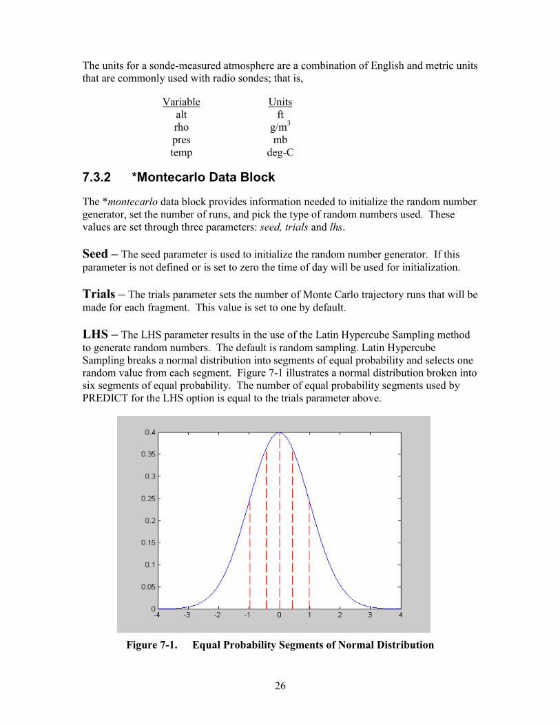
LHS – The LHS parameter results in the use of the Latin Hypercube Sampling method to generate random numbers. The default is random sampling. Latin Hypercube Sampling breaks a normal distribution into segments of equal probability and selects one random value from each segment. Figure 7-1 illustrates a normal distribution broken into six segments of equal probability. The number of equal probability segments used by PREDICT for the LHS option is equal to the trials parameter above.

Figure 7-1. Equal Probability Segments of Normal Distribution

27

7.3.3 *Wind Data Block

Atmospheric winds with respect to the earth’s surface are defined with a *wind data block. If a *wind data block is not input all wind velocities are set to zero. By default wind components are aligned with the geodetic coordinate system. The wind is only a function of altitude and has no vertical component. All units are assumed to be in ft and ft/sec. The east wind component is positive when the wind is from the east (moving from east to west). The north component is positive when the wind is from the north (moving from north to south).

The next parameter in the *wind data block is the file name of the wind table. Four additional parameters can be used inside a *wind data block. They are the standard deviation multipliers fixed_sigma, sigma_north, sigma_east, and sigma_max. These parameters should be followed by their desired value.

Fixed_Sigma – The fixed_sigma parameter sets the east and north standard deviation multipliers to a fixed value (e.g., three sigma) for all Monte Carlo runs. No random numbers are selected. If this parameter is chosen, the sigma_north, sigma_east and sigma_max parameters should not be used.

Sigma_north – The sigma_north parameter sets the north standard deviation multiplier to a fixed value for all Monte Carlo runs. Random numbers are not selected. If sigma_north is set to zero, mean north winds are used. This parameter may be used with the sigma_east parameter, but the fixed_sigma and sigma_max parameters should not be used. If the sigma_east parameter is specified but the sigma_north parameter is not, then sigma_north is set to zero and mean north winds are used.

Sigma_east – The sigma_east parameter sets the east standard deviation multiplier to a fixed value for all Monte Carlo runs. Random numbers are not selected. If sigma_east is set to zero, mean east winds are used. This parameter may be used with the sigma_north parameter, but the fixed_sigma and sigma_max parameters should not be used. If the sigma_north parameter is specified but the sigma_east parameter is not, then sigma_east is set to zero and mean east winds are used.

Sigma_max – The sigma_max option allows random sampling for the east and north standard deviation multiplier but limits the random number to the maximum value entered. This option is useful when the user wants to limit the winds to �3�. If this parameter is chosen, the sigma_north, sigma_east and fixed_sigma parameters should not be used.

7.3.3.1 Wind Table Format

The format of a wind table is as follows:

28

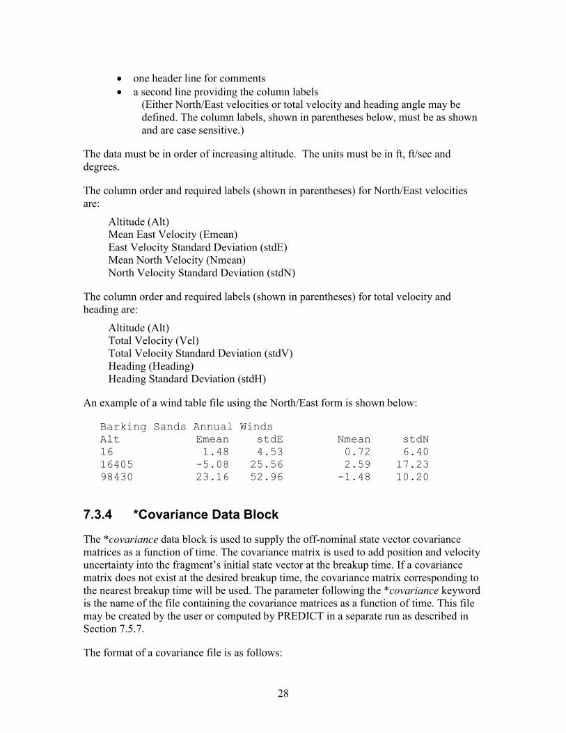
�� one header line for comments �� a second line providing the column labels

(Either North/East velocities or total velocity and heading angle may be defined. The column labels, shown in parentheses below, must be as shown and are case sensitive.)

The data must be in order of increasing altitude. The units must be in ft, ft/sec and degrees.

The column order and required labels (shown in parentheses) for North/East velocities are:

Altitude (Alt) Mean East Velocity (Emean) East Velocity Standard Deviation (stdE) Mean North Velocity (Nmean) North Velocity Standard Deviation (stdN)

The column order and required labels (shown in parentheses) for total velocity and heading are:

Altitude (Alt) Total Velocity (Vel) Total Velocity Standard Deviation (stdV) Heading (Heading) Heading Standard Deviation (stdH)

An example of a wind table file using the North/East form is shown below:

Barking Sands Annual Winds Alt Emean stdE Nmean stdN 16 1.48 4.53 0.72 6.40 16405 -5.08 25.56 2.59 17.23 98430 23.16 52.96 -1.48 10.20

7.3.4 *Covariance Data Block

The *covariance data block is used to supply the off-nominal state vector covariance matrices as a function of time. The covariance matrix is used to add position and velocity uncertainty into the fragment’s initial state vector at the breakup time. If a covariance matrix does not exist at the desired breakup time, the covariance matrix corresponding to the nearest breakup time will be used. The parameter following the *covariance keyword is the name of the file containing the covariance matrices as a function of time. This file may be created by the user or computed by PREDICT in a separate run as described in Section 7.5.7.

The format of a covariance file is as follows:

29

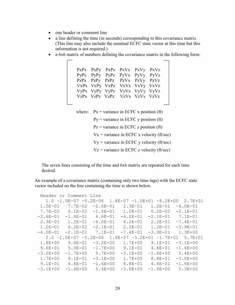
�� one header or comment line �� a line defining the time (in seconds) corresponding to this covariance matrix

(This line may also include the nominal ECFC state vector at this time but this information is not required.)

�� a 6x6 matrix of numbers defining the covariance matrix in the following form:

where: Px = variance in ECFC x position (ft)

Py = variance in ECFC y position (ft)

Pz = variance in ECFC z position (ft)

Vx = variance in ECFC x velocity (ft/sec)

Vy = variance in ECFC y velocity (ft/sec)

Vz = variance in ECFC z velocity (ft/sec)

The seven lines consisting of the time and 6x6 matrix are repeated for each time desired.

An example of a covariance matrix (containing only two time tags) with the ECFC state vector included on the line containing the time is shown below.

Header or Comment Line 1.0 –1.0E-07 –5.2E-06 1.8E-07 –1.5E+01 –8.2E+00 2.7E+01 1.5E-01 7.7E-02 -2.6E-01 2.3E-01 1.2E-01 -4.0E-01 7.7E-02 4.1E-02 -1.4E-01 1.2E-01 6.2E-02 -2.1E-01 -2.6E-01 -1.4E-01 4.6E-01 -4.0E-01 -2.1E-01 7.1E-01 2.3E-01 1.2E-01 -4.0E-01 4.2E-01 2.2E-01 -7.4E-01 1.2E-01 6.2E-02 -2.1E-01 2.2E-01 1.2E-01 -3.9E-01 -4.0E-01 -2.1E-01 7.1E-01 -7.4E-01 -3.9E-01 1.3E+00 2.0 –1.0E-07 –5.2E-06 1.8E-07 –3.2E+01 –1.7E+01 5.7E+01 1.8E+00 9.6E-01 -3.2E+00 1.7E+00 9.1E-01 -3.1E+00 9.6E-01 5.0E-01 -1.7E+00 9.1E-01 4.8E-01 -1.6E+00 -3.2E+00 -1.7E+00 5.7E+00 -3.1E+00 -1.6E+00 5.4E+00 1.7E+00 9.1E-01 -3.1E+00 1.7E+00 8.8E-01 -3.0E+00 9.1E-01 4.8E-01 -1.6E+00 8.8E-01 4.6E-01 -1.6E+00 -3.1E+00 -1.6E+00 5.4E+00 -3.0E+00 -1.6E+00 5.3E+00

PxPx PxPy PxPz PxVx PxVy PxVzPyPx PyPy PyPz PyVx PyVy PyVzPzPx PzPy PzPz PzVx PzVy PzVzVxPx VxPy VxPz VxVx VxVy VxVzVyPx VyPy VyPz VyVx VyVy VyVzVzPx VzPy VzPz VzVx VzVy VzVz

30

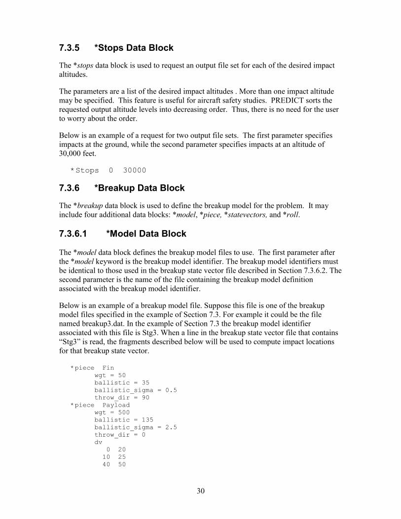
7.3.5 *Stops Data Block

The *stops data block is used to request an output file set for each of the desired impact altitudes.

The parameters are a list of the desired impact altitudes . More than one impact altitude may be specified. This feature is useful for aircraft safety studies. PREDICT sorts the requested output altitude levels into decreasing order. Thus, there is no need for the user to worry about the order.

Below is an example of a request for two output file sets. The first parameter specifies impacts at the ground, while the second parameter specifies impacts at an altitude of 30,000 feet.

*Stops 0 30000

7.3.6 *Breakup Data Block

The *breakup data block is used to define the breakup model for the problem. It may include four additional data blocks: *model, *piece, *statevectors, and *roll.

7.3.6.1 *Model Data Block The *model data block defines the breakup model files to use. The first parameter after the *model keyword is the breakup model identifier. The breakup model identifiers must be identical to those used in the breakup state vector file described in Section 7.3.6.2. The second parameter is the name of the file containing the breakup model definition associated with the breakup model identifier.

Below is an example of a breakup model file. Suppose this file is one of the breakup model files specified in the example of Section 7.3. For example it could be the file named breakup3.dat. In the example of Section 7.3 the breakup model identifier associated with this file is Stg3. When a line in the breakup state vector file that contains “Stg3” is read, the fragments described below will be used to compute impact locations for that breakup state vector.

*piece Fin wgt = 50 ballistic = 35 ballistic_sigma = 0.5 throw_dir = 90 *piece Payload wgt = 500 ballistic = 135 ballistic_sigma = 2.5 throw_dir = 0 dv 0 20 10 25 40 50

31

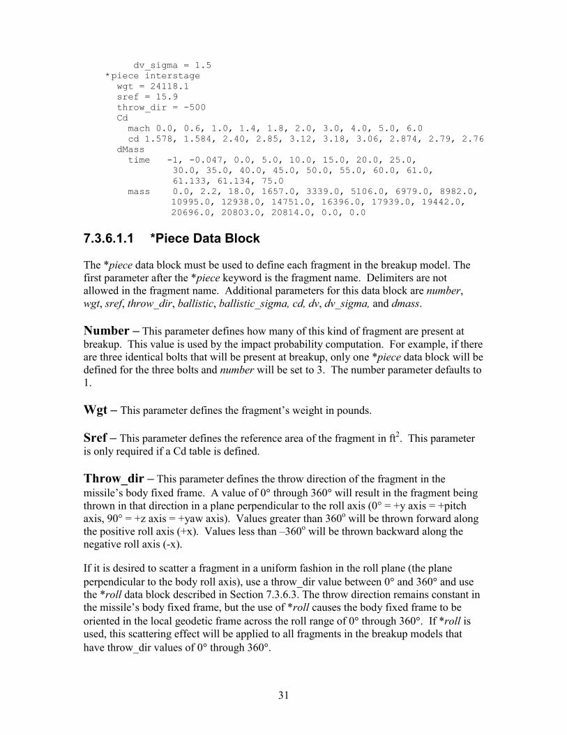
dv_sigma = 1.5 *piece interstage wgt = 24118.1 sref = 15.9 throw_dir = -500 Cd mach 0.0, 0.6, 1.0, 1.4, 1.8, 2.0, 3.0, 4.0, 5.0, 6.0 cd 1.578, 1.584, 2.40, 2.85, 3.12, 3.18, 3.06, 2.874, 2.79, 2.76 dMass time -1, -0.047, 0.0, 5.0, 10.0, 15.0, 20.0, 25.0, 30.0, 35.0, 40.0, 45.0, 50.0, 55.0, 60.0, 61.0, 61.133, 61.134, 75.0 mass 0.0, 2.2, 18.0, 1657.0, 3339.0, 5106.0, 6979.0, 8982.0,

10995.0, 12938.0, 14751.0, 16396.0, 17939.0, 19442.0, 20696.0, 20803.0, 20814.0, 0.0, 0.0

7.3.6.1.1 *Piece Data Block The *piece data block must be used to define each fragment in the breakup model. The first parameter after the *piece keyword is the fragment name. Delimiters are not allowed in the fragment name. Additional parameters for this data block are number, wgt, sref, throw_dir, ballistic, ballistic_sigma, cd, dv, dv_sigma, and dmass.

Number – This parameter defines how many of this kind of fragment are present at breakup. This value is used by the impact probability computation. For example, if there are three identical bolts that will be present at breakup, only one *piece data block will be defined for the three bolts and number will be set to 3. The number parameter defaults to 1.

Wgt – This parameter defines the fragment’s weight in pounds.

Sref – This parameter defines the reference area of the fragment in ft2. This parameter is only required if a Cd table is defined.

Throw_dir – This parameter defines the throw direction of the fragment in the missile’s body fixed frame. A value of 0� through 360� will result in the fragment being thrown in that direction in a plane perpendicular to the roll axis (0° = +y axis = +pitch axis, 90° = +z axis = +yaw axis). Values greater than 360o will be thrown forward along the positive roll axis (+x). Values less than –360o will be thrown backward along the negative roll axis (-x).

If it is desired to scatter a fragment in a uniform fashion in the roll plane (the plane perpendicular to the body roll axis), use a throw_dir value between 0� and 360� and use the *roll data block described in Section 7.3.6.3. The throw direction remains constant in the missile’s body fixed frame, but the use of *roll causes the body fixed frame to be oriented in the local geodetic frame across the roll range of 0� through 360�. If *roll is used, this scattering effect will be applied to all fragments in the breakup models that have throw_dir values of 0� through 360�.

32

Ballistic – The ballistic parameter defines the ballistic coefficient for the fragment in lbf/ft2. As an alternative to defining a ballistic coefficient, a drag coefficient table versus Mach number may be defined (see Cd parameter below).

Ballistic_sigma – This parameter defines the variability in the ballistic coefficient. The ballistic coefficient is determined by adding the input ballistic coefficient (ballistic parameter above) to the input variation multiplied by a uniform random number. If this parameter does not appear the ballistic coefficient is held constant.

Cd – This parameter is used to define the drag force coefficient table to be applied to the fragment as a function of Mach number. If this parameter is used the Sref parameter must be defined. The table format is a Mach number entry followed by the Cd entry. If a Cd table is defined, it will override any entries made through the ballistic and ballistic_sigma parameters. If no extrapolation outside the table is desired, always define a Mach number level above the highest level and repeat the previous table value. Use the same approach for the lowest Mach number level with a repetition of the first table value.

Dv – This parameter is used to define a table containing the incremental velocity applied to the fragment in ft/sec as a function of time. The table is linearly interpolated for a velocity increment at the current state vector time. If no extrapolation outside the table is desired, always define a time after the final time and repeat the previous table value. Use the same approach for the earliest time with a repetition of the first table value.

Dv_sigma – This parameter defines the variability to be applied to the delta velocity table (Dv parameter).

Dmass – This parameter is used to define the mass loss table to be applied to the fragment in pounds vs. time. The table is linearly interpolated for a delta mass for the current state vector time. The fragment’s weight is then reduced by the value determined from the table interpolation. The table format is a time entry followed by the mass loss entry. If no extrapolation outside the table is desired, always define a time after the final time and repeat the previous table value. Use the same approach for the earliest time with a repetition of the first table value.

7.3.6.2 *Statevectors Data Block The *statevectors data block is used to define the state vector at breakup. The first parameter is the file name of the breakup state vector file. The only limit to the number of breakup state vectors that can be included in the state vector file is the memory limit on the particular computer being used.

The format of the state vector file is as follows:

�� two header lines for comments and labels �� data for each breakup state vector (Data are assumed to be in the local geodetic

coordinate frame. Units are in seconds, ft, ft/sec and degrees. Euler angles are

33

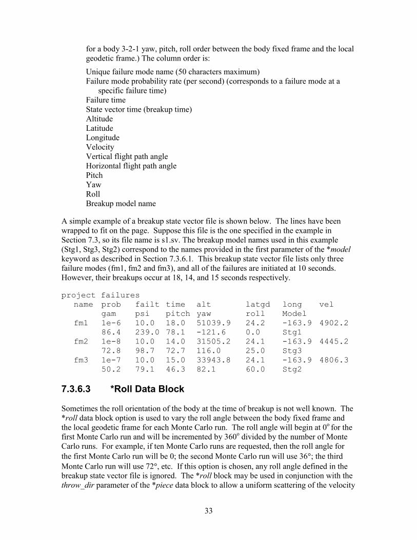
for a body 3-2-1 yaw, pitch, roll order between the body fixed frame and the local geodetic frame.) The column order is:

Unique failure mode name (50 characters maximum) Failure mode probability rate (per second) (corresponds to a failure mode at a

specific failure time) Failure time State vector time (breakup time) Altitude Latitude Longitude Velocity Vertical flight path angle Horizontal flight path angle Pitch Yaw Roll Breakup model name

A simple example of a breakup state vector file is shown below. The lines have been wrapped to fit on the page. Suppose this file is the one specified in the example in Section 7.3, so its file name is s1.sv. The breakup model names used in this example (Stg1, Stg3, Stg2) correspond to the names provided in the first parameter of the *model keyword as described in Section 7.3.6.1. This breakup state vector file lists only three failure modes (fm1, fm2 and fm3), and all of the failures are initiated at 10 seconds. However, their breakups occur at 18, 14, and 15 seconds respectively.

project failures name prob failt time alt latgd long vel gam psi pitch yaw roll Model fm1 1e-6 10.0 18.0 51039.9 24.2 -163.9 4902.2 86.4 239.0 78.1 -121.6 0.0 Stg1 fm2 1e-8 10.0 14.0 31505.2 24.1 -163.9 4445.2 72.8 98.7 72.7 116.0 25.0 Stg3 fm3 1e-7 10.0 15.0 33943.8 24.1 -163.9 4806.3 50.2 79.1 46.3 82.1 60.0 Stg2

7.3.6.3 *Roll Data Block Sometimes the roll orientation of the body at the time of breakup is not well known. The *roll data block option is used to vary the roll angle between the body fixed frame and the local geodetic frame for each Monte Carlo run. The roll angle will begin at 0o for the first Monte Carlo run and will be incremented by 360o divided by the number of Monte Carlo runs. For example, if ten Monte Carlo runs are requested, then the roll angle for the first Monte Carlo run will be 0; the second Monte Carlo run will use 36�; the third Monte Carlo run will use 72�, etc. If this option is chosen, any roll angle defined in the breakup state vector file is ignored. The *roll block may be used in conjunction with the throw_dir parameter of the *piece data block to allow a uniform scattering of the velocity

34

increment in the roll plane across a fragment’s Monte Carlo runs. See Section 7.3.6.1.1 for more information on this approach.

7.3.7 *Intercept Data Block

The *intercept data block is used to define a missile intercept case. Either the KIDD2 or FASTT3 breakup models may be chosen.

7.3.7.1 *FASTT Data Block The data required for the FASTT option are specified with the following parameters:

Min_dia – This parameter defines the minimum diameter fragment to generate in units of meters.

Min_mass – This parameter defines the minimum mass fragment to generate in units of kilograms.

Target, Interceptor – Target and Interceptor have a common set of parameters described below.

Wgt –This parameter defines the target or interceptor weight in kilograms.

Time – This parameter defines the target or interceptor state vector time in seconds.

ECFC – This parameter defines the target or interceptor ECFC state vector in km and km/sec. This parameter is followed by values defining the ECFC state vector position and velocity x, y, z components.

7.3.7.2 *KIDD Data Block The data required for the KIDD option are specified with the following parameters:

Intercept_time – This parameter defines the time of the intercept in seconds.

Fragchoice – This parameter defines the minimum fragment type to be defined by the parameter Cutoffval. 1 = minimum fragment mass, 2 = minimum fragment size.

Cutoffval – This parameter defines the minimum size of fragment produced. The units are defined by the Fragchoice parameter. If Fragchoice = 1, the value is the minimum mass in kilograms. If Fragchoice = 2, the value is the minimum fragment size in meters.

Yaw – This parameter is the first angle (in degrees) of a body 3-2-1 Euler rotation set between the target’s body fixed frame and the ECIC frame. (The ECIC frame is the same frame used in the RV_eci and KV_eci parameters below).

35

Pitch – This parameter is the second angle (in degrees) of a body 3-2-1 Euler rotation set between the ECIC frame and the target’s body fixed frame.

Roll – This parameter is the third angle (in degrees) of a body 3-2-1 Euler rotation set between the ECIC frame and the target’s body fixed frame.

RV_dia – This parameter defines the maximum diameter of the target in meters.

RV_mass – This parameter defines the mass of the target in kilograms.

RV_size – This parameter defines the maximum dimension of the target in meters.

RV_eci – This parameter defines the target ECIC position and velocity components in meters and meters/second. The order is x position, y position, z position, x velocity, y velocity, z velocity.

Nmat_rv – This parameter defines the number of material/thickness combinations for the target. This value is the number of entries to be read for the next three parameters. The maximum number of combinations is 20.

Materid_rv – This parameter defines the target’s material ID array. Aluminum = 1; Uranium = 2; Iron = 3; Silica Phenolic = 4.

Materthick_rv – This parameter defines the target’s average material thickness (m) for each of the material combinations.

Materfrac_rv – This parameter defines the fraction of the target mass for each material combination. The sum of these values must equal 1.

KV_dia – This parameter defines the maximum diameter of the interceptor in meters.

KV_mass – This parameter defines the mass of the interceptor in kilograms.

KV_size – This parameter defines the maximum dimension of the interceptor in meters.

KV_eci – This parameter defines the interceptor ECIC position and velocity components in meters and meters/second.

Nmat_kv – This parameter defines the number of material/thickness combinations for the interceptor. This value is the number of entries to be read for the next three parameters. The maximum number of combinations is 20.

Materid_kv – This parameter defines the material ID array. Aluminum = 1; Uranium = 2; Iron = 3; Silica Phenolic = 4.

36

Materthick_kv – This parameter defines the interceptor’s average material thickness (m) for each of the material combinations.

Materfrac_kv – This parameter defines the fraction of the interceptor mass for each material combination. The sum of these values must equal 1.

Min_beta – This parameter defines the minimum ballistic coefficient (kg/m2) fragment to be included in the impact data.

The following defaults are used by PREDICT when it calls the KIDD program:

Mass conservation, kinetic energy calculations, mass integration for bins, and explicit scaled momentum conservation are turned on. There are no thermal energy calculations, thermal calculations, or high-explosive detonations. The RV is modeled as a strategic nuclear warhead with no booster attached. A lethal hit with a zero miss distance is assumed.

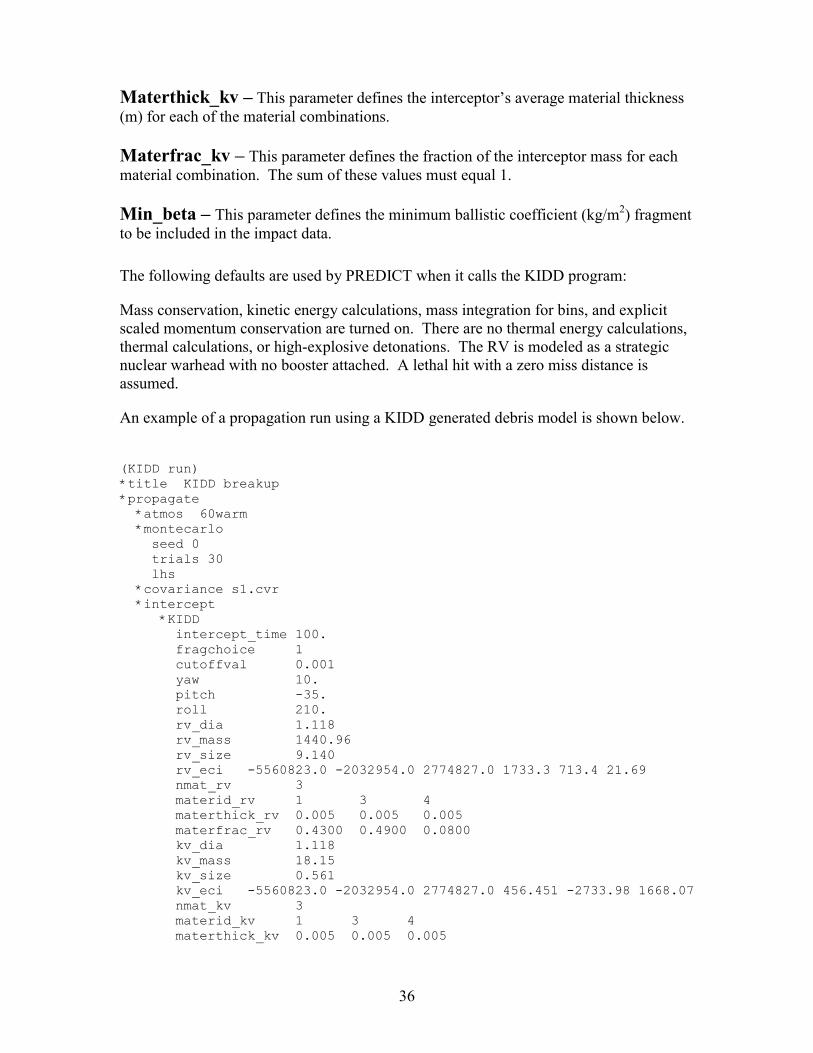
An example of a propagation run using a KIDD generated debris model is shown below.

(KIDD run) *title KIDD breakup *propagate *atmos 60warm *montecarlo seed 0 trials 30 lhs *covariance s1.cvr *intercept *KIDD intercept_time 100. fragchoice 1 cutoffval 0.001 yaw 10. pitch -35. roll 210. rv_dia 1.118 rv_mass 1440.96 rv_size 9.140 rv_eci -5560823.0 -2032954.0 2774827.0 1733.3 713.4 21.69 nmat_rv 3 materid_rv 1 3 4 materthick_rv 0.005 0.005 0.005 materfrac_rv 0.4300 0.4900 0.0800 kv_dia 1.118 kv_mass 18.15 kv_size 0.561 kv_eci -5560823.0 -2032954.0 2774827.0 456.451 -2733.98 1668.07 nmat_kv 3 materid_kv 1 3 4 materthick_kv 0.005 0.005 0.005

37

materfrac_kv 0.450 0.180 0.370 min_beta 0.1 *stops 0 *end

7.4 *PDF Data Block

The *pdf keyword is used to define an impact probability calculation problem. This data block has several sub data blocks: *files, *options, *include, *contours, *plot, *minmv, *minke, *time, and *popcenter. Immediately following the *pdf data block should be a value representing the altitude level at which to compute the impact probabilities. If no value is provided, a warning is issued and the altitude level is set to 0 feet.

An example of a problem file that executes a PDF run only is shown below. The altitude of interest is ground level since the *pdf keyword specifies an altitude of zero. The six impact location files listed have been created by an earlier PREDICT run. The latitude, longitude grid of interest is set up and the desired output file name to be used by the Tecplot� plotting program is provided.

(problem B) *title range safety *pdf 0 *files BK_Stg1-FT_2-ALT_0.pdf BK_Stg1-FT_4-ALT_0.pdf BK_Stg1-FT_6-ALT_0.pdf BK_Stg1-FT_8-ALT_0.pdf BK_Stg1-FT_10-ALT_0.pdf BK_Stg1-FT_12-ALT_0.pdf *options *pdfgrid minLatitude 18.0 maxLatitude 58.0 incLatitude 0.1 minLongitude -154.0 maxLongitude -122.0 incLongitude 0.1 *plot S1_nowind_0.dat *end

7.4.1 *Files Data Block

This data block defines the input files to use in impact probability calculations. This keyword is followed by a list of the impact location file names to use. This data block is not required if a *propagate is defined in the problem prior to this *pdf data block. In that case, the impact location data files generated during the propagation section will be used to supply the impact probability calculations.

38

7.4.2 *Options Data Block

This data block defines the options to use in the definition of the computational grid for the impact probability calculations.

*PdfGrid – This parameter indicates that the user is defining the computation grid. The values are in degrees. The definition parameters are MinLatitude, MaxLatitude, IncLatitude, MinLongitude, MaxLongitude, IncLongitude, StartLatitude, EndLatitude, StartLongitude, EndLongitude, and Width.

MinLatitude – This parameter defines the most southerly latitude of the PdfGrid region.

MaxLatitude – This parameter defines the most northerly latitude of the PdfGrid region.

IncLatitude – This parameter defines the latitude increment of the PdfGrid region.

MinLongitude – This parameter defines the most westerly longitude of the PdfGrid region.

MaxLongitude – This parameter defines the most easterly longitude of the PdfGrid region.

IncLongitude – This parameter defines the longitude increment of the PdfGrid region.

StartLatitude – This parameter defines the beginning latitude of a computation box.

EndLatitude – This parameter defines the ending latitude of a computation box.

StartLongitude – This parameter defines the beginning longitude of a computation box.

EndLongitude – This parameter defines the ending longitude of a computation box.

Width – This parameter defines the width of a computation box.

There are two methods for defining the computation grid. Either the lower left and upper right corners are defined or starting and stopping points with a width are defined. In either case, the step size or increment must be defined.

Most contour plotting packages require a grid of data over the entire region of interest. The simplest method for defining the computational grid is to define the box that will be

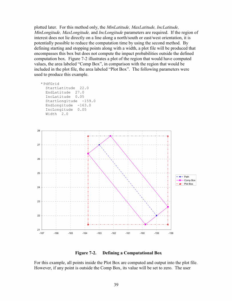
39

plotted later. For this method only, the MinLatitude, MaxLatitude, IncLatitude, MinLongitude, MaxLongitude, and IncLongitude parameters are required. If the region of interest does not lie directly on a line along a north/south or east/west orientation, it is potentially possible to reduce the computation time by using the second method. By defining starting and stopping points along with a width, a plot file will be produced that encompasses this box but does not compute the impact probabilities outside the defined computation box. Figure 7-2 illustrates a plot of the region that would have computed values, the area labeled “Comp Box”, in comparison with the region that would be included in the plot file, the area labeled “Plot Box”. The following parameters were used to produce this example.

*PdfGrid StartLatitude 22.0 EndLatitude 27.0 IncLatitude 0.05 StartLongitude -159.0 EndLongitude -163.0 IncLongitude 0.05 Width 2.0

Figure 7-2. Defining a Computational Box

For this example, all points inside the Plot Box are computed and output into the plot file. However, if any point is outside the Comp Box, its value will be set to zero. The user

21

22

23

24

25

26

27

28

-167 -166 -165 -164 -163 -162 -161 -160 -159 -158

PathComp BoxPlot Box

40

may also define the Plot Box by defining the MaxLatitude, MinLatitude, MaxLongitude, and MinLongitude. A warning is issued to inform the user if the requested Plot Box does not encompass the entire Comp Box. This method is useful when values over a specific grid are required but reduced computational time is desired.

7.4.3 *Include Data Block

This data block defines special input files to be included in the plot output file. These files may be map files of surface features that the user wishes to display on any post-processed plots to be produced. Any files to be included must be in the format required by the plotting software package. This keyword is followed by a list of the file names to be appended to the plot output file.

7.4.4 *Contours Data Block

This data block defines the output file names and contour levels produced. PREDICT will extract contours for each requested contour level and place the latitude and longitude coordinates in the desired output file. Each file name should be followed by a value denoting the desired contour level. The only other option for this keyword is the scale parameter.

Scale – PREDICT currently outputs impact probability data in units of number of impacts per 32 ft2. The user may override this default value. The value supplied should be in the units of impacts/ft2. For example, if a contour plot representing impacts/1000 ft2 were desired the entry would be:

Scale 1000

7.4.5 *Plot Data Block

This data block defines the output file names to use for the plotting software package selected. Currently, only the Tecplot� plotting software format is supported. Conversions to the format used by the RRAT program are discussed in Section 7.5.5.

7.4.6 *Minke Data Block

The *minke data block defines the minimum kinetic energy fragment to be considered in the impact probability calculations. If this option is not defined, no screening will be performed, and all impact locations will be used.

7.4.7 *Minmv Data Block

The *minmv data block defines the minimum mass*velocity fragment to be considered in the impact probability calculations. If this option is not defined, no screening will be performed, and all impact locations will be used.

41

7.4.8 *Time Data Block

The *time data block defines the times at which to compute an impact probability grid. This data block is used to produce time varying impact probability plots used in the evaluation of aircraft safety. There are two input sets for this keyword, the times at which to produce the plots and their corresponding time ranges. These sets are defined by the parameters times and dt. For example, the following input would produce one impact probability plot based on all fragments that fall through 35,000 ft between 400 and 600 seconds (500 seconds +/- 100 seconds) and another impact probability plot for the fragments that fall through 35,000 ft between 700 and 1700 seconds (1200 seconds +/- 500 seconds).

*Pdf 35000 *Time times 500 1200 dt 100 500

If this data block is not present in the problem definition, then the impact probability plot produced will be time independent and will represent the impacts from all debris. If this data block is defined, the plot file names, defined by the *plot keyword described in Section 7.4.5, will be modified by the addition of the time value.

7.4.9 *Popcenter Data Block

This data block defines the file name of a list of population centers (e.g., boats, buildings) used to compute the probability of impact and casualty expectations. The first parameter is the name of the input file containing the population center information. The second parameter is the desired output file name.

The format of the population center input file follows:

�� two header lines for comments and labels (After these two header lines any lines with a ‘#’ as the first character are taken as comments and copied directly into the output file.)

�� data with column order: Longitude (deg) Latitude (deg) Reference Area (ft2) Population Size Limit

The format of the output file is as follows:

�� a copy of the first header line from the input file �� the output data with column order:

(The first five columns are duplicates of the input file values.)

42

Longitude (deg) Latitude (deg) Reference area (ft2) Population size Limit Impact probability (impacts/reference area) Casualty expectation Maximum population that will still meet the defined limit

An example of an input file is shown below. The fishing boat in this example is assumed to carry 10 people and have a reference area of 1000 ft2. The probability of impact limit for this type of population center is 1e-6.

Population Centers Longitude Latitude Ref_Area Pop_Size Limit # Fishing Boat -159.722 22.178 1000 10 1e-6 # Skycreen -159.765944 22.070528 32 1 1e-5 # Range Assets -159.781256 22.061879 10000 1 1e-3 # Beach -159.761 22.088 32 20 1e-6 -159.754 22.094 32 10 1e-6

7.5 *Tools Data Block

The *tools data block is used to post-process some of the output data. The allowable data blocks following *tools are *popcenter, *union, *contours, *path, *rrat, *tecplot, and *covariance. The *tools data block has not been set up to operate in a parallel processing environment so only one processor is used for this data block.

7.5.1 *Popcenter Data Block

This data block defines the file name of a list of population centers to compute the probability of impact and casualty expectations. This data block is similar to that defined in Section 7.4.9. The definition parameters are Pdf, Centers, and Output.

Pdf – This parameter defines the impact probability file to be used to compute the probability of impact and expected casualties for the input population centers.

Centers – This parameter defines the population centers input file name. The format of the input file is as follows:

�� two header lines for comments and labels (After these two header lines any lines with a ‘#’ as the first character are taken as comments and copied directly into the output file.)

�� data with column order:

43

Longitude (deg) Latitude (deg) Reference Area (ft2) Population Size Limit

Output – This parameter defines the name of the output file. The format of the output file is as follows:

�� a copy of the first header line from the input file

�� a line of column headers �� the data with the following column order (the first five columns are duplicates

from the input file): Longitude (deg) Latitude (deg) Reference area (ft2) Population size Limit Impact probability (impacts/reference area) Casualty expectation Maximum population that will still meet the defined limit

A problem file example for this tool is given below.

(casualties) *tools *popcenter pdf nearlaunch.dat centers pop.dat output pop.out *end

The file named nearlaunch.dat is an impact probability file generated from a PREDICT *pdf run. The population center file pop.dat has the same form as the input file shown in Section 7.4.9.

7.5.2 *Union Data Block

This data block defines a combination of multiple impact probability files into one file. The combination may be accomplished either by adding the probability of impact values from each file at corresponding grid points using the *add data block or by searching the files to find the maximum probability of impact value at each grid point using the *max data block. Both *add and *max have the same definition parameters: files, output, minLatitude, maxLatitude, incLatitude, minLongitude, maxLongitude, and incLongitude. If minLatitude, maxLatitude, incLatitude, minLongitude, maxLongitude, and incLongitude are not defined, the output file’s size will correspond to the size of the largest dimensions and smallest increment of the input files.

44

Files – This parameter provides the list of impact probability files to be combined.

Output – This parameter defines the name of the combined file. This file will be in Tecplot© format and the size will correspond to the extremes of all the input impact probability files and the smallest increment.

MinLatitude – This parameter defines the most southerly latitude of the output file.

MaxLatitude– This parameter defines the most northerly latitude of the output file.

IncLatitude – This parameter defines the latitude increment of the output file.

MinLongitude – This parameter defines the most westerly longitude of the output file.

MaxLongitude – This parameter defines the most easterly longitude of the output file.

IncLongitude – This parameter defines the longitude increment of the output file.

An example of a problem file using the *add data block is shown below.

(union example) *title PROJECT A *tools *union *add files S1_nowind_0.dat1a S1_nowind_0.dat1b S1_nowind_0.dat1c S1_nowind_0.dat1d output nowind_0.dat *end

7.5.3 *Contours Data Block

This data block defines a tool to compute the probability of impact and casualty expectations for either a specific trajectory or an estimated simple trajectory based on a set of input parameters. The definition parameters are Pdf, Scale, and Output.

Pdf – This parameter defines the impact probability file to be used to compute the data for the input population centers.

45

Scale – This parameter defines the area used for the contour computations. For example, if a contour plot representing the number of impacts/1000 ft2 were desired the entry would be:

Scale 1000

Output – This parameter defines the name of the output file followed by the contour level value. The output file consists of a set of longitude and latitude points defining the contour. If more than one contour at this level is present, the individual fragments will be separated by a blank line.

7.5.4 *Path Data Block

This tool is used in risk to aircraft studies by inputting either the aircraft’s known trajectory or its projected trajectory based on knowledge of its path at one instant in time. The definition parameters are Files, Projected, Points, and Output.

Files – This parameter defines the list of impact probability files to be used. These files must have been previously computed for the altitudes and the latitude/longitude grids the aircraft will be traversing.

Projected – This option is used if only minimal information is known about the aircraft’s trajectory. PREDICT computes the aircraft’s path and uses that information to get probability of impact and casualty expectations for the aircraft.

This parameter provides the name of the file containing the starting point information. The format of this file is as shown below.

�� one header line �� data in the following column order:

Time Alt Long Lat Vel Heading VFPA dT maxT Ref Area Pop

where: Time = current time (sec) Alt = current altitude (ft) Long = current longitude (deg) Lat = current latitude (deg) Vel = current velocity (knots) Heading = current heading angle (deg) VFPA = current vertical flight path angle (deg) dT = desired delta time for path computation maxT = maximum time to compute path over Ref Area = reference area of this object (ft2) Pop = population of this object

A problem file example for this option is shown below. The five files listed are impact probability files computed by PREDICT for five time baskets using the *time

46

feature described in section 7.4.8. One point of the aircraft’s trajectory is provided in file projpath.dat in the format described above.

(test proj path) *tools *path files nowind_30k_T-325.dat nowind_30k_T-555.dat nowind_30k_T-785.dat nowind_30k_T-1015.dat nowind_30k_T-1245.dat projected projpath.dat output projpath.out *end

Points – This option is used if the aircraft’s path is known. This parameter provides the name of the file containing the aircraft’s trajectory. The format for this file is as shown below.

�� one header line �� data in the following column order:

Time Alt Long Lat Ref Area Pop (See Projected parameter above for descriptions of these entities.)

A problem file example for this option is shown below. The five files listed are impact probability files computed by PREDICT for five time baskets using the *time feature described in Section 7.4.8. The aircraft’s trajectory is provided in file AC_traj.dat in the format described above.

(aircraft) *tools *path files nowind_30k_T-325.dat nowind_30k_T-555.dat nowind_30k_T-785.dat nowind_30k_T-1015.dat nowind_30k_T-1245.dat points AC_traj.dat output AC_ecpi.out *end

Output – This parameter defines the name of the output file. The output file format will be as shown below.

�� repeat of input file header line �� column headers:

Time Altitude Longitude Latitude Pi Ec | Cum Pi Cum Ec �� output data

47

Each successive line will contain either the time, altitude, longitude, and latitude provided in a points file or the data computed from the projected file inputs. The Pi column is the impact probability computed at that instant in time. The Ec column is the casualty expectation based on the computed Pi and the provided population. The Cum Pi and Cum Ec are running totals for the previous two columns.

7.5.5 *RRAT Data Block

This tool is used to convert a Tecplot© formatted impact probability data file into a set of files in the format used by the RRAT code developed by ACTA. RRAT can only accept maximum increments of 500 in either latitude or longitude. Thus, the incLatitude and incLongitude parameters are set internally to comply with this requirement. The two output files generated have the same name as the output file with “-Pi.grd” and “-Ec.grd” added to the end of the file name. If no Output block is defined the Tecplot© file name is used. The definition parameters are Tecplot, minLatitude, maxLatitude, minLongitude, maxLongitude, Output, Ec, Tecplot_scale, and Ec_scale.

Tecplot – This parameter defines the input file name. This file name should be the 32 ft2 file produced by PREDICT that is read by Tecplot© to produce contour plots.

MinLatitude – This parameter defines the most southerly latitude of the output file.

MaxLatitude – This parameter defines the most northerly latitude of the output file.

MinLongitude – This parameter defines the most westerly longitude of the output file.

MaxLongitude – This parameter defines the most easterly longitude of the output file.

Output – This parameter defines the name of the output file. The Pi output file contains seven “layers” of data that are needed by the SIMDIS plot program developed by the Naval Research Laboratory. The first and second layers correspond to 1000 ft2. The third through seventh layers correspond to three times the area of the previous layer. For example the third layer corresponds to 3000 ft2, the fourth layer to 9000 ft2, etc. The Ec output file is only one layer deep and corresponds to 1000 ft2 if no Tecplot_scale or Ec_scale inputs are used.

Ec – This parameter flags the program to only generate an Ec file using the scale factors defined below.

Tecplot_scale – This parameter defines the scale factor for the input Tecplot© file. The default value for this scale factor is number of impacts/32 ft2. This scale factor is only used if the Ec flag is set.

48

Ec_scale – This parameter defines the scale factor for the output Ec file. This scale factor is only used if the Ec flag is set.

A problem file example for this tool is shown below for no Ec scaling.

(conversion to RRAT) *title rrat_grid *tools *RRAT Tecplot nowind_0.dat MinLatitude 18.0 MaxLatitude 58.0 MinLongitude -154.0 MaxLongitude -122.0 *end

7.5.6 *TECPLOT Data Block

This tool converts an RRAT formatted impact probability data file into a Tecplot© formatted data file. The definition parameters are RRAT, Ec, Pi, Alt, Time, and Tecplot.

RRAT – This parameter defines the input RRAT formatted file name.

Ec – This parameter defines the RRAT formatted file as an Ec file type.

Pi – This parameter defines the RRAT formatted file as a Pi file type.

Alt – This parameter defines the altitude of the RRAT formatted file.

Time – This parameter defines the time of the RRAT formatted file. The value supplied may be the time of the RRAT file or the value UNDEF for a time independent file.

Tecplot – This parameter defines the output Tecplot© formatted file name.

7.5.7 *Covariance Data Block

This data block defines a tool to compute a covariance matrix based on a set of off-nominal trajectories. See Section 7.3.4 for more information on the covariance input file. The definition parameters are Nominal, Offnominal, Tmin, Tmax, and Output.

Nominal – This parameter defines the name of the nominal trajectory input file. If this file is not defined, a nominal trajectory will be based on the average of the off-nominal trajectories. If a nominal trajectory is supplied, the format is the same as the off-nominal trajectory format in the Offnominal parameter section.

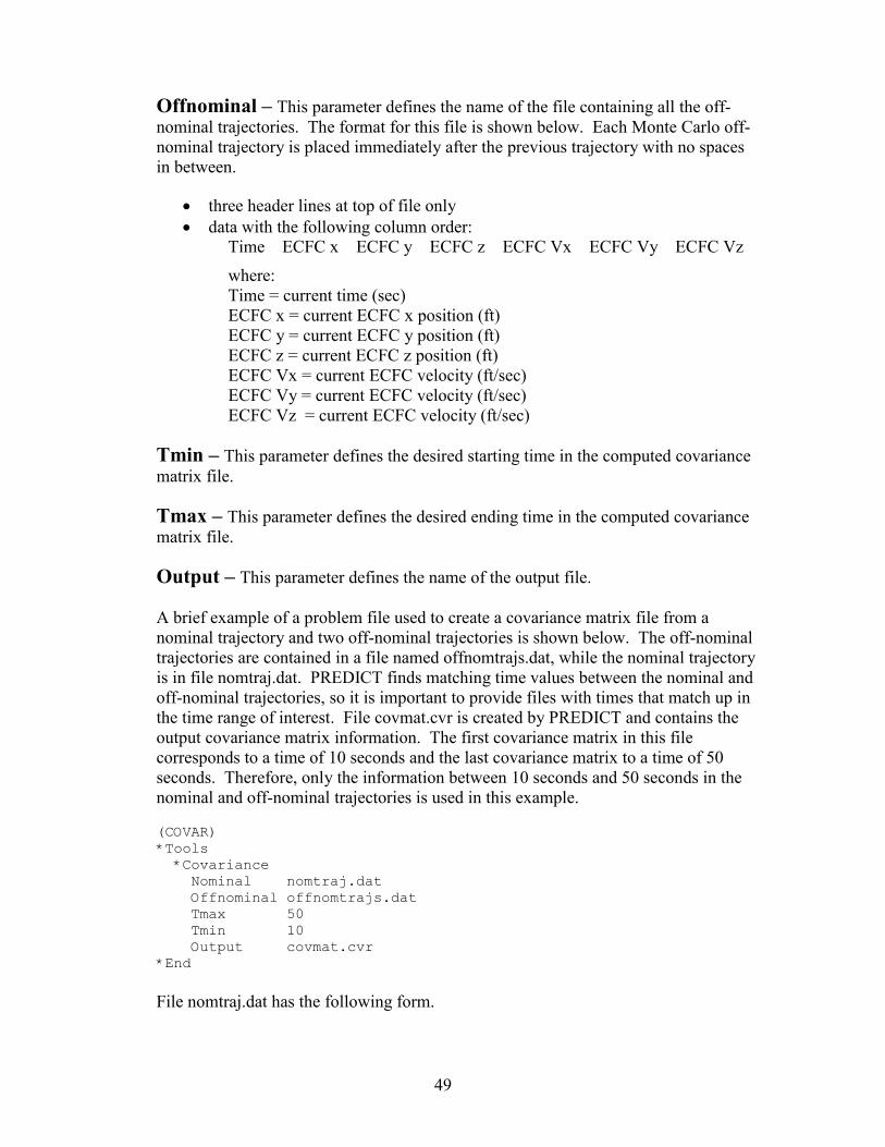
49

Offnominal – This parameter defines the name of the file containing all the off-nominal trajectories. The format for this file is shown below. Each Monte Carlo off-nominal trajectory is placed immediately after the previous trajectory with no spaces in between.

�� three header lines at top of file only �� data with the following column order:

Time ECFC x ECFC y ECFC z ECFC Vx ECFC Vy ECFC Vz

where: Time = current time (sec) ECFC x = current ECFC x position (ft) ECFC y = current ECFC y position (ft) ECFC z = current ECFC z position (ft) ECFC Vx = current ECFC velocity (ft/sec) ECFC Vy = current ECFC velocity (ft/sec) ECFC Vz = current ECFC velocity (ft/sec)

Tmin – This parameter defines the desired starting time in the computed covariance matrix file.

Tmax – This parameter defines the desired ending time in the computed covariance matrix file.

Output – This parameter defines the name of the output file. A brief example of a problem file used to create a covariance matrix file from a nominal trajectory and two off-nominal trajectories is shown below. The off-nominal trajectories are contained in a file named offnomtrajs.dat, while the nominal trajectory is in file nomtraj.dat. PREDICT finds matching time values between the nominal and off-nominal trajectories, so it is important to provide files with times that match up in the time range of interest. File covmat.cvr is created by PREDICT and contains the output covariance matrix information. The first covariance matrix in this file corresponds to a time of 10 seconds and the last covariance matrix to a time of 50 seconds. Therefore, only the information between 10 seconds and 50 seconds in the nominal and off-nominal trajectories is used in this example.

(COVAR) *Tools *Covariance Nominal nomtraj.dat Offnominal offnomtrajs.dat Tmax 50 Tmin 10 Output covmat.cvr *End File nomtraj.dat has the following form.

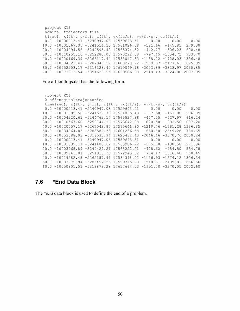
50

project XYZ nominal trajectory file t(sec), x(ft), y(ft), z(ft), vx(ft/s), vy(ft/s), vz(ft/s) 0.0 -10000213.41 -5240947.08 17559643.51 0.00 0.00 0.00 10.0 -10001067.35 -5241514.10 17561026.08 -181.66 -145.81 279.38 20.0 -10004094.56 -5244595.48 17565374.52 -442.77 -506.23 600.48 30.0 -10010255.16 -5252280.08 17573292.08 -797.45 -1054.72 983.70 40.0 -10020169.39 -5266117.44 17585017.83 -1188.22 -1728.03 1356.48 50.0 -10034021.47 -5287045.57 17600270.92 -1589.37 -2477.63 1695.09 60.0 -10052203.17 -5316228.49 17619049.18 -2023.89 -3328.97 2030.85 70.0 -10073213.54 -5351629.95 17639506.98 -2219.43 -3824.80 2097.95 File offnomtrajs.dat has the following form. project XYZ 2 off-nominaltrajectories time(sec), x(ft), y(ft), z(ft), vx(ft/s), vy(ft/s), vz(ft/s) 0.0 -10000213.41 -5240947.08 17559643.51 0.00 0.00 0.00 10.0 -10001095.50 -5241539.76 17561065.43 -187.60 -153.08 286.89 20.0 -10004220.61 -5244762.17 17565527.88 -457.05 -527.97 616.24 30.0 -10010567.60 -5252744.16 17573642.08 -820.50 -1092.56 1007.20 40.0 -10020757.17 -5267042.85 17585641.90 -1219.46 -1781.28 1386.85 50.0 -10034964.83 -5288584.33 17601236.58 -1630.80 -2549.28 1734.65 60.0 -10053588.03 -5318533.94 17620432.43 -2046.46 -3370.76 2050.24 0.0 -10000213.41 -5240947.08 17559643.51 0.00 0.00 0.00 10.0 -10001039.11 -5241488.62 17560986.72 -175.70 -138.58 271.86 20.0 -10003968.89 -5244429.21 17565222.01 -428.62 -484.50 584.78 30.0 -10009943.01 -5251815.30 17572943.32 -774.47 -1016.68 960.45 40.0 -10019582.48 -5265187.91 17584398.02 -1156.93 -1674.12 1326.34 50.0 -10033079.94 -5285497.55 17599315.20 -1548.31 -2405.81 1656.56 60.0 -10050801.51 -5313873.28 17617664.03 -1991.78 -3270.05 2002.60

7.6 *End Data Block

The *end data block is used to define the end of a problem.

51

References 1. D. E. Salguero, Trajectory Analysis and Optimization Software (TAOS), SAND99-

0811 Revised, Sandia National Laboratories, Albuquerque, NM, June 2001.

2. KIDD Kernel Version 3.5.3, Report No. N-TR-99-052, Nichols Research, Huntsville,

AL, April 1999.

3. McKnight, D., Maher, R., and Nagl, L., Fragmentation Algorithms for Strategic and

Theater Targets (FASTT) Empirical Breakup Model, Ver 3.0, DNA-TR-94-104, December 1994.

52

Distribution: 2 Commander NAWCWD

Code 521300E 575 I Ave. Suite 1 Point Mugu, CA 93042-5049 Attn. J. Morris

3 Commander Navy Region Hawaii

Care Of Pacific Missile Range Facility Attention: Code N814 Box 128 Kekaha, HI 96752-0128 Attn. S. Hudson Code 7331

1 William A. Millard

450 Sunnyside Ridge Road Sandpoint, ID 83864 1 MS 0825 T. M. Jordan-Culler, 15414 1 MS 0825 M. W. Kniskern, 15414 1 MS 0825 L. R. Rollstin, 15414 10 MS 1174 W. H. Rutledge, 15414 10 MS 0825 B. R. Sturgis, 15414 1 MS 0825 W. P. Wolfe, 9115 10 MS 0933 L. W. Young, 10823 1 MS 9018 Central Technical Files, 8945-1 2 MS 0899 Technical Library, 9616 1 MS 0612 Review & Approval Desk, 9612 for DOE/OSTI 1 MS 0161 Patent & Licensing Office, 11500