Predicting 2016 State Presidential Election Results

with a National Tracking Poll and MRP

Chad P. Kiewiet de Jonge*

Gary Langer†

May 26, 2017

ABSTRACT

This paper presents state-level estimates of the 2016 presidential election using data from the

ABC News and ABC News/Washington Post tracking poll and multilevel regression with

poststratification (MRP). The multilevel models employ basic demographic variables at the

individual level (gender, age, education and race) and a few state-level variables (past turnout,

past party vote shares and the shares of blacks, Hispanics and evangelical white Protestants in

each state’s population), to estimate group-level turnout and vote preferences. Poststratification

on 2015 American Community Survey estimates of demographic group sizes in each state results

in correct predictions of the winner in 50 of 51 states and the District of Columbia (missing only

Michigan) using data from 9,485 Americans interviewed in the weeks leading up to the election.

While the approach does not perfectly estimate turnout as a share of the voting age population,

popular vote shares or vote margins in each state, the model is more accurate than predictions

published by polling aggregators or other MRP estimators, including in the number of races

correctly projected and the root mean square error on the Clinton-Trump margin across states.

The paper also reports how vote preferences changed over the course of the 18-day tracking

period, compares subgroup-level estimates of turnout and vote preferences with the 2016

National Election Pool exit poll and summarizes the accuracy of the approach applied to the

2000, 2004, 2008 and 2012 elections. The paper concludes by discussing how researchers can

make use of MRP as an alternative approach to survey weighting and likely voter modeling as

well as in forecasting future elections.

Presented at the annual conference of the

American Association for Public Opinion Research

New Orleans, Louisiana, Saturday, May 20, 2017‡

* Senior research analyst, Langer Research Associates (New York) and affiliated professor of the division

of political studies at the Center for Research and Teaching in Economics (Mexico City). † President, Langer Research Associates (New York). ‡ The chart and footnote on p.20 have been updated from the conference paper.

I. OVERVIEW

Donald Trump’s widely unexpected victory in the 2016 U.S. presidential election has

raised questions about the accuracy of public opinion polling, the aggregation of polling into

probabilistic election forecasts and the interpretation of election polling by data analysts,

journalists and the general public. While national-level polls on average proved as accurate as in

past elections in predicting the popular vote (with an average error on the margin of about 2

points), there were substantial polling errors at the state level, particularly in Midwestern swing

states (Eten 2016; Silver 2017; Cohn, Katz and Quealy 2016). These significant misses,

amplified by a proliferation of overconfident probabilistic forecasts, have (fairly or not) placed a

cloud over the polling industry, provided ammunition to critics of survey research and led the

leading industry association to study how the 2016 misses can be avoided in the future. This

paper demonstrates the advantages of a statistical approach developed over the past two decades,

multilevel regression with poststratification (MRP), in improving survey estimates in general

and, specifically, in producing superior forecasts of election outcomes.

Our use of MRP combines statistical modeling of national-level survey data with census

estimates of demographic group sizes at the state level to produce state-level turnout and

candidate preference estimates (Park, Gelman and Bafumi 2004; Lax and Phillips 2009a, 2009b;

Pacheco 2011; Ghitza and Gelman 2013). By combining individual-level demographic and state-

level predictors of turnout and candidate preferences, the technique leverages subgroup-level

similarities in electoral attitudes across geographical units (in this case, states). Through this

partial pooling approach, MRP can provide highly accurate state-level estimates of voter

intentions even with relatively small state-level sample sizes.

3

We focus chiefly on our implementation of MRP using survey data from the 2016 ABC

News and ABC News/Washington Post tracking poll,1 a national, probability-based RDD survey

of the general public. We use data from 18 days of interviews leading up to the 2016 election

among 9,485 adults overall and 7,778 self-reported registered voters, with a median state sample

size of 133.2 Using this dataset, the models correctly predict the presidential winner in 50 of the

51 states and the District of Columbia, missing only Michigan, which was decided by 10,407

votes out of 4.8 million cast. The analysis estimates the national popular vote margin within

four-tenths of a percentage point and produces lower errors on the Clinton-Trump margin across

states than leading polling aggregators and non-probability 50-state polls.3 We obtain similar

results from analyses of ABC News and ABC/Post tracking data from the previous four

presidential elections, demonstrating the robustness of the approach.

More than solely a predictive enterprise, the MRP analysis also sheds light on the

dynamics of the 2016 race, in terms of trends over time and voting behavior among demographic

groups. Except for the first four days of the tracking poll Oct. 20-23, the model found Trump

ahead in the Electoral College even as he generally trailed Clinton in the popular vote. Notably,

the narrowing of the race occurred prior to FBI Director James Comey’s Oct. 28 letter to

Congress reopening the controversy over Clinton’s use of a private email server as secretary of

1 The Post did not participate in the poll’s first five days of interviews. 2 The AAPOR response rate 3 for the full survey was 15.6 percent, including a cooperation rate (AAPOR

3) of 38.7 percent. 3 We developed the model experimentally during the election; minor subsequent refinements included the

use of more recent census data, elimination of a phone-status adjustment and addition of a time-trend

adjustment. These changes had little effect. Our results were not publicly released prior to the election; as

such we present this analysis solely as a proof of the utility of the approach, not as a claim to have made a

public prediction.

4

state – an important analytical finding, given subsequent commentary blaming Clinton’s loss on

the Comey letter.

Our MRP analysis suggests that the electorate was older, slightly whiter and less well

educated than suggested by the National Election Pool (NEP) national exit poll, and that

Trump’s victory among white voters was narrower than the exit poll suggests, with more-

educated whites in particular more strongly for Clinton than in the exit poll. Given the exit poll’s

unadjusted or noisily adjusted group-level nonresponse, MRP likely provides a more accurate

picture.

We proceed with the following sections: First, an overview of the motivation for MRP

modeling and the statistical strategy employed for this analysis. Second, a description of the data

used in the analysis. Third, turnout and candidate support estimates by state. Fourth, analysis of

the race nationally and a discussion of group-level dynamics. Fifth, results of similar analyses

using tracking poll data from the four previous presidential elections. Fifth, discussion of

strengths and weaknesses of our approach, with suggestions for future research.

II. USING MRP FOR STATE-LEVEL ESTIMATES

Motivation

National-level surveys proved at least as accurate in 2016 as they have been in past

elections – only slightly misstating the popular vote (overestimating Clinton’s victory over

Trump by 1-2 points), and more accurate on average than in 2012 (Silver 2017; Cohn, Katz and

Quealy 2016). But state-level polling painted a different and ultimately much more inaccurate

picture of the race. Trump prevailed in the Electoral College by narrowly winning primarily

5

Midwestern swing states where polling averages suggested that Clinton was ahead. Observers

have pointed to a number of potential explanations for the large errors in state-level polling

(Mercer, Deane and Kyley 2016). While disentangling these explanations is not the objective of

this paper, the state poll misses do raise the specter of similar errors in the future.

MRP constitutes a promising alternative, avoiding uncertain rigor in state polls and the

need for prescience in anticipating where to conduct them. Instead, MRP in this analysis relies

on national-level survey data, in combination with statistical modeling and census data, to

generate state-level estimates of voter turnout and candidate choice. The approach takes

advantage of the fact that MRP can provide highly accurate state-level estimates of attitudes and

behaviors even with relatively small number of observations in each state.

The statistical properties and substantive advantages of MRP have been discussed in

detail elsewhere.4 Researchers start with a national-level survey dataset, preferably with a fairly

large number of observations. A multilevel statistical model predicting the outcome of interest is

fit, using basic demographic variables that are available in census data at the state (or other

subnational unit) level. Additional state-level variables can be included in the model in an effort

to sharpen estimates. Coefficients for continuous variables usually are unmodeled (i.e., fixed),

while group variables are modeled as categorical random effects. In the case of election-

preference estimates, multiple models are required, first estimating the likelihood of voting,

followed by additional model(s) estimating candidate preferences.

4 See Park, Gelman and Bafumi (2004), Ghitza and Gelman (2013), Lax and Phillips (2009a, 2009b),

Pacheco (2011) and Wang et al. (2014).

6

In the second stage of MRP analysis, the model estimates are used to predict the outcome

variable for groups defined in a poststratification dataset. This dataset has an observation

corresponding to each group defined for all combinations of the demographic variables included

in the model. For example, if the model includes U.S. states/D.C. (n=51), gender (n=2) and a

four-category race/ethnicity variable (n=4), the poststratification dataset will have 51*2*4= 408

rows, and will include the population size in each group from census estimates. After predicting

the outcome variable for each of the groups in the poststratification dataset, estimates can be

aggregated to the state (or other subgroup unit) level, with the subgroup population sizes

determining the relative weight of each group’s estimate in the state-level estimate.

MRP provides a powerful approach to generating state-level opinion estimates by pooling

information from similar groups in other states, in effect leveraging subgroup-level attitudinal

homogeneity (as established in regression analysis). Through multilevel modeling, results among

multiple groups are partially pooled; for example, the prediction for Hispanic men living in

Oregon will be informed by the outcome among similar Hispanic men in other states, other

people living in Oregon, men across the country, Hispanics across the country, etc.

The degree to which estimates are partially pooled across groups is largely dependent on

sample sizes; with larger samples, group estimates more closely reflect the outcome in the data,

while estimates for smaller sample size groups are more dependent on the model (i.e.,

information provided by similar groups). Thus, pooling of data across states is particularly

important for states with smaller sample sizes; estimates from states with larger sample sizes rely

more on the survey data and less on the statistical model.

7

MRP is likely to prove most valuable relative to other approaches when particular

features of the data hold true. First, MRP is most useful with moderately large national-level

datasets – large enough to produce adequate state-level samples but not so large that those

samples can stand alone. Second, moderate variation in the outcome variable across geographical

subunits is desirable. If the outcome does not vary across states, classical regression would

suffice; if the outcome varies greatly across states, partial pooling may be no better than

disaggregation or classical regression (Gelman and Hill 2009, 247). Third, MRP works best

when the demographic variables available for poststratification strongly predict the outcome; if

they do not, estimates are likely to be poor (Lax and Phillips 2009b). In the case of modern

American presidential elections, all three of these features hold true.

Statistical Strategy

As noted above, using MRP to predict election preferences by state requires estimating

both propensity to vote, and candidate choice, among groups. In our analysis, starting first with

candidate preferences, two sets of multilevel logistic regression models predicting preference for

Clinton or Trump, respectively, were fit, with respondents preferring the other major-party

candidate, a third-party candidate, or undecided set to 0.

The candidate preference equations are as follows:

Pr(𝑐𝑎𝑛𝑑𝑖𝑑𝑎𝑡𝑒𝑖𝑗) = logit−1(𝛼0 + 𝛽1(2012 𝑝𝑎𝑟𝑡𝑦 𝑠ℎ𝑎𝑟𝑒) + 𝛽2(𝑏𝑙𝑎𝑐𝑘 𝑠ℎ𝑎𝑟𝑒) +

𝛽3(𝐻𝑖𝑠𝑝𝑎𝑛𝑖𝑐 𝑠ℎ𝑎𝑟𝑒) + 𝛽4(𝑤ℎ𝑖𝑡𝑒 𝑒𝑣𝑎𝑛𝑔. 𝑠ℎ𝑎𝑟𝑒)+𝛼1𝑔𝑒𝑛𝑑𝑒𝑟

+

𝛼2𝑎𝑔𝑒5

+ 𝛼3𝑟𝑎𝑐𝑒4 + 𝛼4

𝑒𝑑𝑢5 + 𝛼5𝑠𝑡𝑎𝑡𝑒 + 𝛼6

𝑟𝑒𝑔𝑖𝑜𝑛+ 𝛼7

𝑎𝑔𝑒5,𝑒𝑑𝑢5+

8

𝛼8𝑔𝑒𝑛𝑑𝑒𝑟,𝑒𝑑𝑢5

+ 𝛼9𝑟𝑎𝑐𝑒5,𝑎𝑔𝑒5

+ 𝛼10𝑟𝑎𝑐𝑒5,𝑒𝑑𝑢5 + 𝛼11

𝑟𝑎𝑐𝑒5,𝑔𝑒𝑛𝑑𝑒𝑟+

𝛼12𝑟𝑎𝑐𝑒,𝑟𝑒𝑔𝑖𝑜𝑛

+ 𝛼13𝑤𝑎𝑣𝑒) (1)

In this equation, 𝛼0 is the baseline intercept, while the remaining alpha coefficients correspond to

variance components for the grouping variables, which include typical survey weighting

variables (gender, age, education and race/ethnicity), geographical factors (state, region), and

interactions between several of these factors (age*education, gender*education, race*age,

race*education, race*gender and race*region). To capture any time trends, a random effect for

time periods in the tracking survey (“waves”) is included. The equation also includes three state-

level variables and associated fixed beta coefficients suggested by previous research by others

and testing with prior ABC/Post data to increase the precision of state-level estimates. These

include the Obama and Romney vote shares in each state, respectively, (Ghitza and Gelman

2013; Wang et al. 2014) and the proportion of each state’s population made up of African-

Americans, Hispanics and evangelical white Protestants. The independent prior distributions for

each of the varying coefficients are normally distributed with zero means and variances

estimated from the data, 𝛼𝑗𝑆~ N (0, (𝜎𝑆)2).

Best approaches for estimating group-level turnout likelihood are less clear. Group-level

turnout has been estimated using data from other surveys related to the previous (or concurrent)

presidential election. Wang et al. (2014) estimated group level turnout in 2012 using 2008 exit

poll data, while others have employed the U.S. Census Bureau’s Current Population Survey

(CPS) voter supplement (Ghitza and Gelman 2013; Lauderdale 2016; Cohn and Cox 2016).

These researchers justify this choice by pointing out that these sources measure reported turnout

9

with probability-based sampling methods and large sample sizes, and argue that turnout rates by

group do not vary substantially across elections.

Of course, if the assumption of constant subgroup turnout across elections does not hold,

then these turnout estimates are likely to prove inaccurate. Given this consideration, we take an

alternative approach, modeling turnout based on each survey respondent’s self-expressed

intention to vote and past reported voting participation. Specifically, respondents who said they

were registered to vote at their current address, would definitely vote or had voted early and

voted in 2012 were classified as voters (=1) while all other respondents were non-voters (=0). Of

three operationalizations of turnout that were tested, this approach produced the most accurate

estimates using previous years’ data. Moreover, it should be noted that the goal was not to

assemble literal voters but rather to predict the probability of turnout among groups, something

this simplified approach accomplishes effectively. As a result, turnout is estimated with a nearly

identical multilevel logistic regression model, with the difference being that the only state level

variable included is the voting age population turnout in each state in 2012:

Pr(𝑣𝑜𝑡𝑒𝑖) = logit−1(𝛼0 + 𝛽1(2012 𝑉𝐴𝑃 𝑡𝑢𝑟𝑛𝑜𝑢𝑡)+𝛼1𝑔𝑒𝑛𝑑𝑒𝑟

+ 𝛼2𝑎𝑔𝑒5

+ 𝛼3𝑟𝑎𝑐𝑒4 + 𝛼4

𝑒𝑑𝑢5

+ 𝛼5𝑠𝑡𝑎𝑡𝑒 + 𝛼6

𝑟𝑒𝑔𝑖𝑜𝑛+ 𝛼7

𝑎𝑔𝑒5,𝑒𝑑𝑢5+ 𝛼8

𝑔𝑒𝑛𝑑𝑒𝑟,𝑒𝑑𝑢5+ 𝛼9

𝑟𝑎𝑐𝑒5,𝑎𝑔𝑒5

+ 𝛼10𝑟𝑎𝑐𝑒5,𝑒𝑑𝑢5 + 𝛼11

𝑟𝑎𝑐𝑒5,𝑔𝑒𝑛𝑑𝑒𝑟+ 𝛼12

𝑟𝑎𝑐𝑒,𝑟𝑒𝑔𝑖𝑜𝑛+ 𝛼13

𝑤𝑎𝑣𝑒)

𝛼𝑗𝑆 ~ N (0, (𝜎𝑆)2) (2)

In the next stage, the turnout model estimates were poststratified on the census dataset,

producing an estimate of the number of Americans in each subgroup who were likely to vote.

The preference model estimates (vote for Clinton, vote for Trump) next were poststratified on

10

the estimated likely voter population in each subgroup. These estimates were adjusted to reflect

time trends by using the final survey wave random effect estimate in the prediction, which

essentially assumes uniform swings5 in turnout/candidate preferences among groups. With these

estimated numbers of voters overall and for each of the two main candidates, estimates of all

three quantities could be aggregated to the state as well as subgroup levels.

III. DATA AND ESTIMATION

The national survey data chiefly used in the analysis is from the 2016 ABC News and

ABC News/Washington Post tracking poll, a probability-based RDD cellular and landline

telephone survey of respondents in the continental United States. We use data collected over 18

days preceding the Nov. 8, 2016, election, ending on Nov. 6. During each of the first 14 days,

approximately 440 members of the general public were interviewed, while about 800 were

interviewed per day on days 15-18, Thursday-Sunday before the election. A total of 9,485

respondents (including 7,778 self-reported registered voters) are included in the dataset, 65

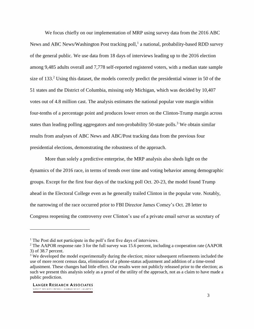
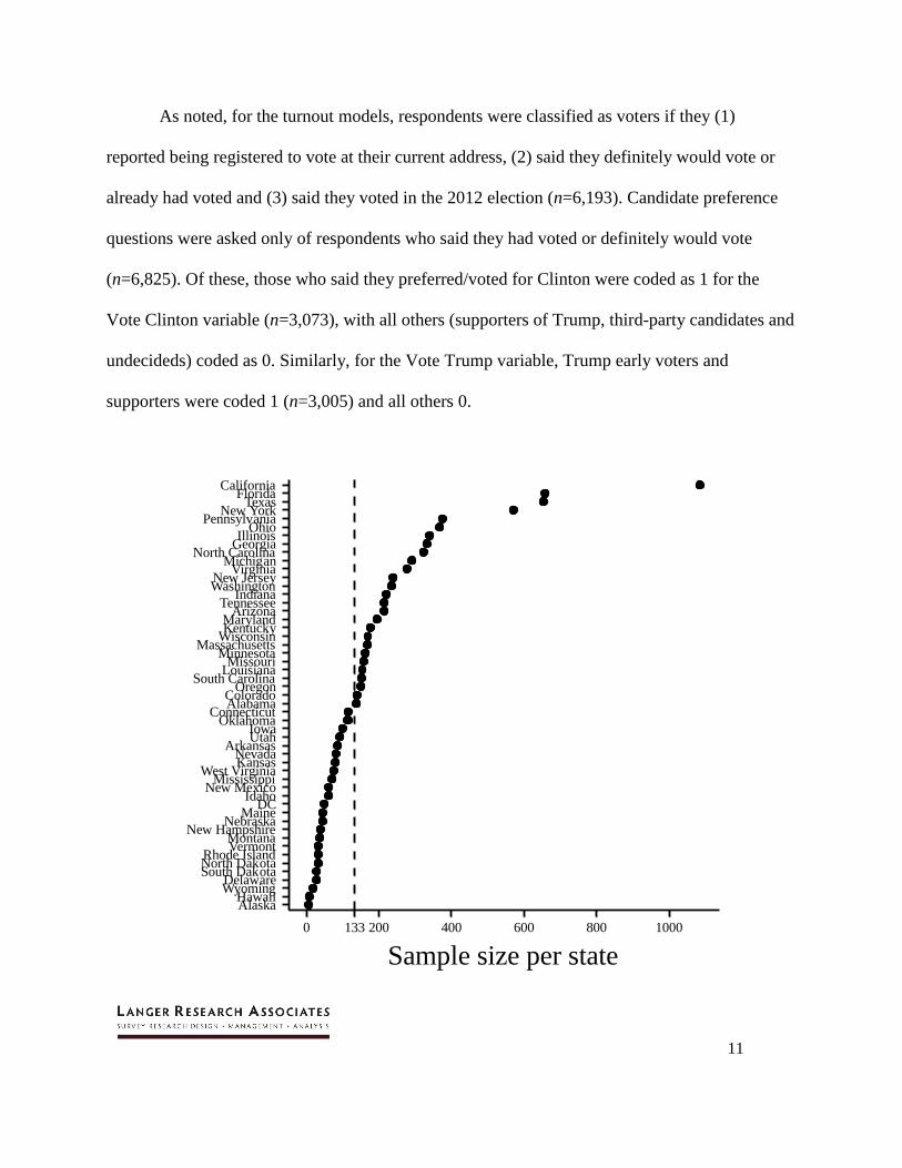
percent of whom were interviewed via cell phone.6 Figure 1 plots the sample size by state,

ranging from six respondents in Alaska7 to 1,084 in California, with the median state (Colorado)

including 133 respondents.

5 The assumption of uniform swings may be a weakness of this approach, but consequential differential

late-stage swings don’t appear to be an issue, given the robustness of our model over time, and reliably

testing time-trend interactions would require larger sample sizes than we have available. 6 Additional methodological details are available at http://abcnews.go.com/US/PollVault/abc-news-

polling-methodology-standards/story?id=145373. 7 Respondents from Alaska and Hawaii only include those reached on cell phones with area codes from

the continental United States.

11

As noted, for the turnout models, respondents were classified as voters if they (1)

reported being registered to vote at their current address, (2) said they definitely would vote or

already had voted and (3) said they voted in the 2012 election (n=6,193). Candidate preference

questions were asked only of respondents who said they had voted or definitely would vote

(n=6,825). Of these, those who said they preferred/voted for Clinton were coded as 1 for the

Vote Clinton variable (n=3,073), with all others (supporters of Trump, third-party candidates and

undecideds) coded as 0. Similarly, for the Vote Trump variable, Trump early voters and

supporters were coded 1 (n=3,005) and all others 0.

AlaskaHawaii

WyomingDelaware

South DakotaNorth DakotaRhode Island

VermontMontana

New HampshireNebraska

MaineDC

IdahoNew Mexico

MississippiWest Virginia

KansasNevada

ArkansasUtahIowa

OklahomaConnecticut

AlabamaColorado

OregonSouth Carolina

LouisianaMissouri

MinnesotaMassachusetts

WisconsinKentuckyMaryland

ArizonaTennessee

IndianaWashingtonNew Jersey

VirginiaMichigan

North CarolinaGeorgiaIllinois

OhioPennsylvania

New YorkTexas

FloridaCalifornia

0 133 200 400 600 800 1000

Sample size per state

12

Figure 1. General population sample sizes per state. The dashed line indicates the

median state sample size. MRP turnout models used this full sample, while

candidate preference models were estimated among those who said they had voted

or definitely would vote.

Demographic group variables included as random effects were gender (male, female),

age (18-29, 30-39, 40-49, 50-64, 65+), race/ethnicity (white non-Hispanic, black non-Hispanic,

Hispanic, and other non-Hispanic),8 and education (less than high school, high school graduate,

some college, four-year college graduate, post-graduate). State of residence was determined by

area code and exchange for landline respondents and asked of cell phone respondents. The

region variable used 13 sociopolitical regions based on state of residence. To capture any time

trends, the tracking period was divided into five periods, the first three of which were four days

in length and the last two at three days each.

Poststratification data were taken from the U.S. Census Bureau’s 2015 American

Community Survey (ACS) one-year estimates, the most recent census data released before the

election. Since the poststratification dataset includes cells for every combination of the

demographic variables included in the model, the dataset contains 10,200 rows with ACS

estimates of the population size in each of these groups.

State-level variables included past voting-age-population turnout estimates compiled by

McDonald (2016), prior vote shares for Obama and Romney in 2012, aggregate racial group

shares from the 2015 ACS estimates and estimates of evangelical white Protestants in each state

from the Public Religion Research Institute’s American Values Atlas (2016).

8 Taking advantage of their larger sample size, the last four days of the tracking period included questions

asking Hispanics whether they were born in the United States or abroad, for more fine-grained weighting.

Models using the resulting five-point race/ethnicity variable produced similar results for this period.

13

For estimates of uncertainty, MRP models can be estimated with full Bayesian methods;

this analyses uses a more approximate maximum likelihood estimator since the focus is on point

estimates. Models were estimated in R using the glmer function in the lme4 package (Bates and

Maechler 2009). After initial model runs, random effects with zero estimated variances were

removed from the models to aid convergence.

IV. 2016 RESULTS

Turnout

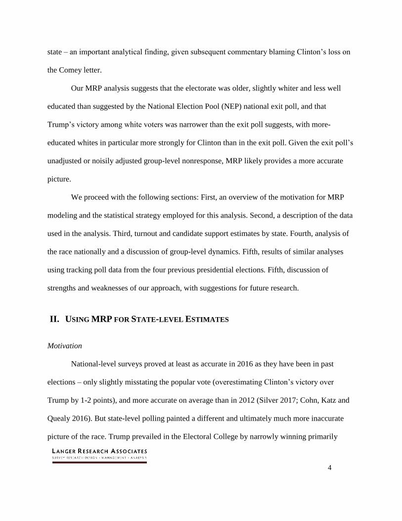
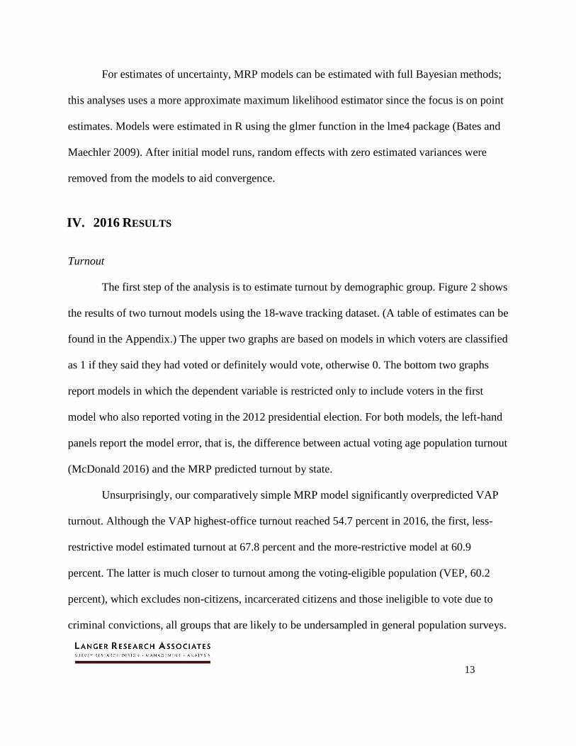
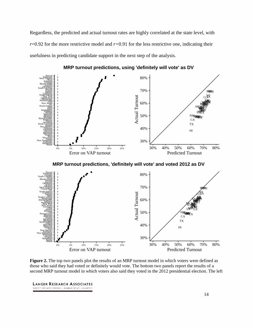
The first step of the analysis is to estimate turnout by demographic group. Figure 2 shows

the results of two turnout models using the 18-wave tracking dataset. (A table of estimates can be

found in the Appendix.) The upper two graphs are based on models in which voters are classified

as 1 if they said they had voted or definitely would vote, otherwise 0. The bottom two graphs

report models in which the dependent variable is restricted only to include voters in the first

model who also reported voting in the 2012 presidential election. For both models, the left-hand

panels report the model error, that is, the difference between actual voting age population turnout

(McDonald 2016) and the MRP predicted turnout by state.

Unsurprisingly, our comparatively simple MRP model significantly overpredicted VAP

turnout. Although the VAP highest-office turnout reached 54.7 percent in 2016, the first, less-

restrictive model estimated turnout at 67.8 percent and the more-restrictive model at 60.9

percent. The latter is much closer to turnout among the voting-eligible population (VEP, 60.2

percent), which excludes non-citizens, incarcerated citizens and those ineligible to vote due to

criminal convictions, all groups that are likely to be undersampled in general population surveys.

14

Regardless, the predicted and actual turnout rates are highly correlated at the state level, with

r=0.92 for the more restrictive model and r=0.91 for the less restrictive one, indicating their

usefulness in predicting candidate support in the next step of the analysis.

Figure 2. The top two panels plot the results of an MRP turnout model in which voters were defined as

those who said they had voted or definitely would vote. The bottom two panels report the results of a

second MRP turnout model in which voters also said they voted in the 2012 presidential election. The left

MRP turnout predictions, using 'definitely will vote' as DV

MaineMinnesota

ColoradoNew Hampshire

AlaskaWisconsin

IowaVirginia

MarylandDelawareVermont

LouisianaMontana

New MexicoOregon

North CarolinaWyoming

IllinoisKentucky

MassachusettsMichiganMissouriNebraska

FloridaAlabama

WashingtonIdahoOhio

North DakotaDC

New JerseyUtah

PennsylvaniaMississippi

ConnecticutNew York

South DakotaCalifornia

IndianaKansasNevada

South CarolinaOklahoma

ArizonaRhode Island

GeorgiaArkansas

TexasWest Virginia

TennesseeHawaii

0% 5% 10% 15% 20% 25%

Error on VAP turnout

ALAK

AZARCA

CO

CTDE

DCFL

GA

HI

IDILIN

IA

KSKYLA

ME

MDMAMI

MN

MS

MOMTNE

NV

NH

NJ

NMNY

NCNDOH

OK

ORPA

RISCSD

TN

TX

UT

VTVAWA

WV

WI

WY

30%

40%

50%

60%

70%

80%

30% 40% 50% 60% 70% 80%

Predicted Turnout

Act

ual

Tu

rnout

MRP turnout predictions, 'definitely will vote' and voted 2012 as DV

MaineAlaska

MinnesotaVirginia

ColoradoWisconsin

New HampshireKentucky

New MexicoIowa

VermontDelawareMaryland

OregonNorth Dakota

MichiganWyoming

FloridaNebraskaMontana

PennsylvaniaUtah

MissouriIllinois

OhioLouisiana

New JerseyNew York

WashingtonAlabama

MassachusettsMississippi

North CarolinaIdaho

IndianaCalifornia

South DakotaDC

ConnecticutWest Virginia

ArkansasKansas

OklahomaArizonaNevada

Rhode IslandTexas

South CarolinaGeorgia

TennesseeHawaii

0% 5% 10% 15% 20% 25%

Error on VAP turnout

ALAK

AZARCA

CO

CTDE

DCFL

GA

HI

IDILIN

IA

KSKYLA

ME

MDMAMI

MN

MS

MOMTNE

NV

NH

NJ

NMNY

NCNDOH

OK

ORPA

RISCSD

TN

TX

UT

VTVA

WA

WV

WI

WY

30%

40%

50%

60%

70%

80%

30% 40% 50% 60% 70% 80%

Predicted Turnout

Act

ual

Turn

ou

t

15

panels plot the model errors by state, with perfect predictions at zero and overpredictions as greater than

zero. The right panels plot the MRP turnout predictions vs. the actual turnout. The models overestimated

turnout in states below the 45-degree line; states for which turnout was overestimated would appear above

the line.

The median absolute model error for the more-restrictive turnout model was 5.6 points.

Errors reached double digits in a few states, with the largest for Hawaii at 13 points (a state not

included in the sampling frame), followed by Tennessee (11 points) and Georgia (11 points).

Turnout errors decreased as the level of actual turnout in each state increased; errors were

minimal in high-turnout states such as Minnesota and Wisconsin. Indeed, the prediction error is

correlated at r = -0.77 with actual turnout. This outcome may reflect a greater likelihood of

voters to answer surveys. However, and important for estimates of national-level candidate

support, turnout prediction errors were essentially uncorrelated with the Clinton-Trump

candidate margins across states (r=0.01). The poststratified estimates of subgroup-level turnout

from the restrictive model were used to identify the number of voters in each subgroup for the

candidate-preference poststratification.

Vote Preference

The next set of models estimated preferences for Clinton (vs. other candidates) and

Trump (vs. other candidates) using a similar set of demographic predictors at the individual

level. To demonstrate the utility of including state-level predictors in the multilevel models, the

first results in the top two panels of Figure 3 are based on models that did not include any state-

level predictors, while the bottom two panels are based on models that also included 2012 vote

16

shares for Obama and Romney and the proportions of blacks, Hispanics and evangelical white

Protestants in each state’s population. Coefficient estimates are given in Appendix A.

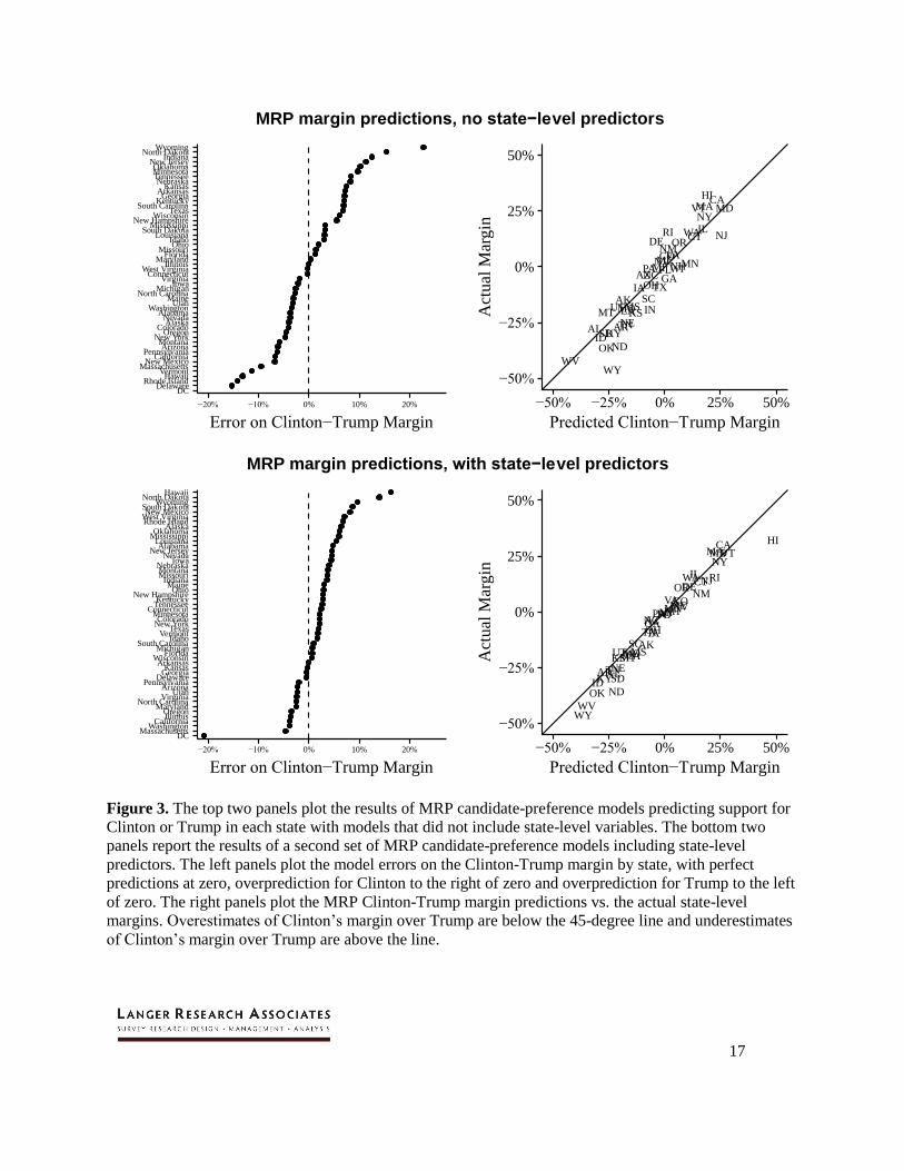
While the MRP estimates for both sets of models were not perfect at the state level,

overall they proved quite accurate. Clinton won the national popular vote by 2.1 points (48.2 to

46.1 percent); the estimates from the MRP models reported in Figure 2 show 2.2- and 2.5-point

Clinton leads, respectively (46.7 to 44.4 percent and 46.8 to 44.3 percent). The models also

proved highly accurate in predicting which candidate would win in each state and fairly accurate

in predicting those vote margins. The first set of models correctly predicted 45 of 51 races (and a

narrow electoral-college victory for Clinton, 275-263). Adding 2012 vote shares (not shown)

increased the number of correct predictions to 47, while the models including aggregate

racial/ethnic shares missed only Michigan, the state with the closest margin.

For all states, the root mean square error (RMSE) on the Clinton-Trump margin for the

second set of models is 5.8 points, dropping to 4.5 points after excluding Hawaii, Alaska and the

District of Columbia. The RMSE for the Clinton and Trump estimates per state for the full model

are 2.3 and 3.5 points (excluding Alaska, Hawaii and D.C.), respectively, indicating quite

accurate point estimates for each candidate. The absolute errors on the Clinton-Trump margins

only reach double digits in three low-population states (Hawaii, North Dakota and Wyoming)

and D.C., while eight state margin estimates are off by 5-10 points (Alaska, Louisiana,

Mississippi, New Mexico, Oklahoma, Rhode Island, South Dakota, and West Virginia).

17

Figure 3. The top two panels plot the results of MRP candidate-preference models predicting support for

Clinton or Trump in each state with models that did not include state-level variables. The bottom two

panels report the results of a second set of MRP candidate-preference models including state-level

predictors. The left panels plot the model errors on the Clinton-Trump margin by state, with perfect

predictions at zero, overprediction for Clinton to the right of zero and overprediction for Trump to the left

of zero. The right panels plot the MRP Clinton-Trump margin predictions vs. the actual state-level

margins. Overestimates of Clinton’s margin over Trump are below the 45-degree line and underestimates

of Clinton’s margin over Trump are above the line.

MRP margin predictions, no state−level predictors

DCDelaware

Rhode IslandHawaii

VermontMassachusetts

New MexicoCalifornia

PennsylvaniaArizona

MontanaNew York

OregonColorado

AlaskaNevada

AlabamaWashington

UtahMaine

North CarolinaMichigan

IowaVirginia

ConnecticutWest Virginia

IllinoisMaryland

FloridaMissouri

OhioIdaho

LouisianaSouth Dakota

MississippiNew Hampshire

WisconsinTexas

South CarolinaKentucky

GeorgiaArkansas

KansasNebraska

TennesseeMinnesotaOklahoma

New JerseyIndiana

North DakotaWyoming

−20% −10% 0% 10% 20%

Error on Clinton−Trump Margin

AL

AK

AZ

AR

CA

CO

CTDE

FLGA

HI

ID

IL

IN

IA

KS

KY

LA

ME

MDMA

MI MN

MSMOMTNE

NVNH

NJ

NM

NY

NC

ND

OH

OK

OR

PA

RI

SC

SDTN

TX

UT

VT

VA

WA

WV

WI

WY−50%

−25%

0%

25%

50%

−50% −25% 0% 25% 50%

Predicted Clinton−Trump Margin

Act

ual

Mar

gin

MRP margin predictions, with state−level predictors

DCMassachusetts

WashingtonCalifornia

IllinoisOregon

MarylandNorth Carolina

VirginiaUtah

ArizonaPennsylvania

DelawareGeorgiaKansas

ArkansasWisconsin

FloridaMichigan

South CarolinaIdaho

VermontTexas

New YorkColorado

MinnesotaConnecticut

TennesseeKentucky

New HampshireOhio

MaineIndiana

MissouriMontanaNebraska

IowaNevada

New JerseyAlabama

LouisianaMississippiOklahoma

AlaskaRhode IslandWest VirginiaNew Mexico

South DakotaWyoming

North DakotaHawaii

−20% −10% 0% 10% 20%

Error on Clinton−Trump Margin

AL

AK

AZ

AR

CA

CO

CTDE

FLGA

HI

ID

IL

IN

IA

KS

KY

LA

ME

MDMA

MIMN

MSMOMTNE

NVNH

NJ

NM

NY

NC

ND

OH

OK

OR

PA

RI

SC

SDTN

TX

UT

VT

VA

WA

WV

WI

WY−50%

−25%

0%

25%

50%

−50% −25% 0% 25% 50%

Predicted Clinton−Trump Margin

Act

ual

Mar

gin

18

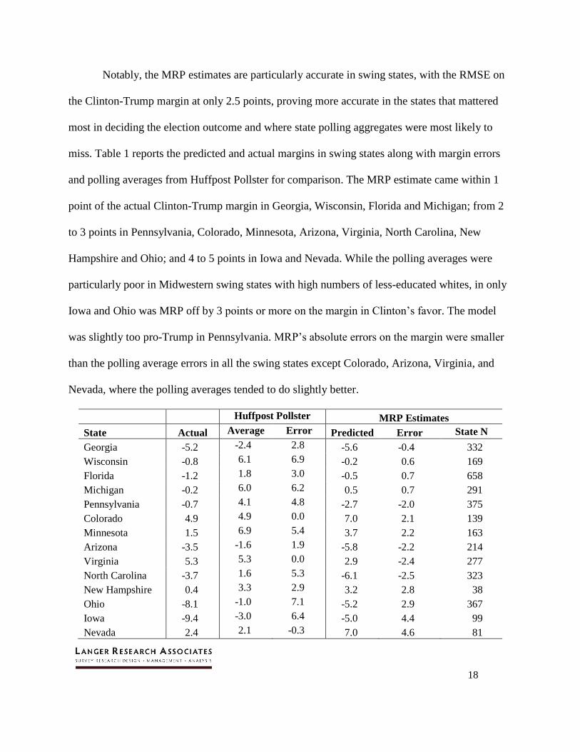
Notably, the MRP estimates are particularly accurate in swing states, with the RMSE on

the Clinton-Trump margin at only 2.5 points, proving more accurate in the states that mattered

most in deciding the election outcome and where state polling aggregates were most likely to

miss. Table 1 reports the predicted and actual margins in swing states along with margin errors

and polling averages from Huffpost Pollster for comparison. The MRP estimate came within 1

point of the actual Clinton-Trump margin in Georgia, Wisconsin, Florida and Michigan; from 2

to 3 points in Pennsylvania, Colorado, Minnesota, Arizona, Virginia, North Carolina, New

Hampshire and Ohio; and 4 to 5 points in Iowa and Nevada. While the polling averages were

particularly poor in Midwestern swing states with high numbers of less-educated whites, in only

Iowa and Ohio was MRP off by 3 points or more on the margin in Clinton’s favor. The model

was slightly too pro-Trump in Pennsylvania. MRP’s absolute errors on the margin were smaller

than the polling average errors in all the swing states except Colorado, Arizona, Virginia, and

Nevada, where the polling averages tended to do slightly better.

Huffpost Pollster MRP Estimates

State Actual Average Error Predicted Error State N

Georgia -5.2 -2.4 2.8 -5.6 -0.4 332

Wisconsin -0.8 6.1 6.9 -0.2 0.6 169

Florida -1.2 1.8 3.0 -0.5 0.7 658

Michigan -0.2 6.0 6.2 0.5 0.7 291

Pennsylvania -0.7 4.1 4.8 -2.7 -2.0 375

Colorado 4.9 4.9 0.0 7.0 2.1 139

Minnesota 1.5 6.9 5.4 3.7 2.2 163

Arizona -3.5 -1.6 1.9 -5.8 -2.2 214

Virginia 5.3 5.3 0.0 2.9 -2.4 277

North Carolina -3.7 1.6 5.3 -6.1 -2.5 323

New Hampshire 0.4 3.3 2.9 3.2 2.8 38

Ohio -8.1 -1.0 7.1 -5.2 2.9 367

Iowa -9.4 -3.0 6.4 -5.0 4.4 99

Nevada 2.4 2.1 -0.3 7.0 4.6 81

19

Table 1. Actual Clinton-Trump margins vs. the Huffpollster polling average and MRP estimates in

swing states.

Comparison to Aggregators

While MRP’s accuracy is impressive, given the closeness of the election in many states

and the RMSEs of the estimates, missing only one state likely was due to chance. However, as

shown in Table 2, our MRP model results outperform the predictions of polling aggregators as

well a sophisticated MRP model that employed a large non-probability online dataset. This is

true not only in terms of the number of states correctly predicted but also in the accuracy of state-

level point estimates.

As noted, our MRP model correctly predicted 50 of 51 contests, vs. 46 correct predictions

for the leading aggregators, 45 for The New York Times’ Upshot and 43 for SurveyMonkey and

YouGov’s MRP model.9 Similarly, the RMSE on the Clinton-Trump margin for our MRP model

is 5.8 points for all states, dropping to 4.5 points after excluding Alaska, Hawaii and D.C. and

2.5 points among battlegrounds. In the comparison models, the RMSE exceeds 7 points for all

states, with no or only marginal improvement when excluding Alaska, Hawaii and D.C.10 Our

MRP model’s RMSE among battleground states also outperforms the comparison models, with

the closest being Fivethirtyeight, with a 3.9-point RMSE for these states (vs. our 2.5). Our

9 Note that the number of correct predictions assumes that the predicted winner in each state is the one

with the higher predicted vote share in that state. Some of the forecasted total electoral vote shares

differed for the aggregator models (e.g., Fivethirtyeight) because electoral votes were simulated

separately. These alternative models also produced estimates for states that allocated electoral votes by

congressional district (Maine and Nebraska), which our MRP model was not designed to accommodate. 10 The improvements in our MRP estimates for these contests reflect the fact that Alaska and Hawaii were

not in the sample frame, while D.C. is an unusual case with few respondents.

20

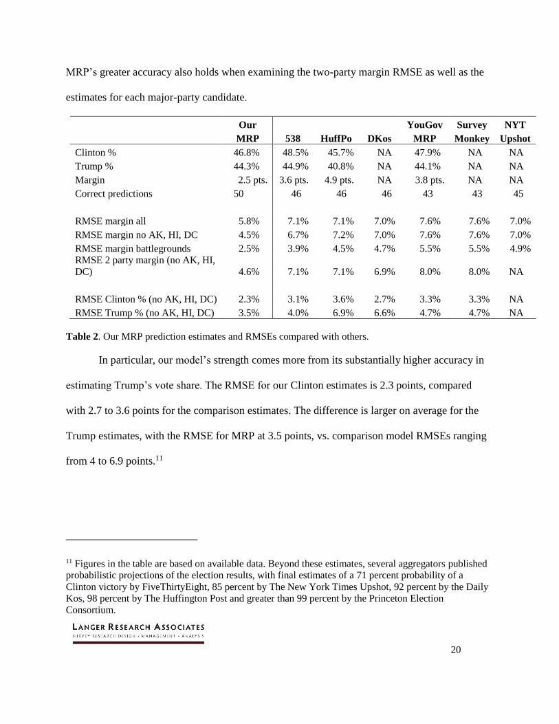
MRP’s greater accuracy also holds when examining the two-party margin RMSE as well as the

estimates for each major-party candidate.

Our YouGov Survey NYT

MRP 538 HuffPo DKos MRP Monkey Upshot

Clinton % 46.8% 48.5% 45.7% NA 47.9% NA NA

Trump % 44.3% 44.9% 40.8% NA 44.1% NA NA

Margin 2.5 pts. 3.6 pts. 4.9 pts. NA 3.8 pts. NA NA

Correct predictions 50 46 46 46 43 43 45

RMSE margin all 5.8% 7.1% 7.1% 7.0% 7.6% 7.6% 7.0%

RMSE margin no AK, HI, DC 4.5% 6.7% 7.2% 7.0% 7.6% 7.6% 7.0%

RMSE margin battlegrounds 2.5% 3.9% 4.5% 4.7% 5.5% 5.5% 4.9%

RMSE 2 party margin (no AK, HI,

DC) 4.6% 7.1% 7.1% 6.9% 8.0% 8.0% NA

RMSE Clinton % (no AK, HI, DC) 2.3% 3.1% 3.6% 2.7% 3.3% 3.3% NA

RMSE Trump % (no AK, HI, DC) 3.5% 4.0% 6.9% 6.6% 4.7% 4.7% NA

Table 2. Our MRP prediction estimates and RMSEs compared with others.

In particular, our model’s strength comes more from its substantially higher accuracy in

estimating Trump’s vote share. The RMSE for our Clinton estimates is 2.3 points, compared

with 2.7 to 3.6 points for the comparison estimates. The difference is larger on average for the

Trump estimates, with the RMSE for MRP at 3.5 points, vs. comparison model RMSEs ranging

from 4 to 6.9 points.11

11 Figures in the table are based on available data. Beyond these estimates, several aggregators published

probabilistic projections of the election results, with final estimates of a 71 percent probability of a

Clinton victory by FiveThirtyEight, 85 percent by The New York Times Upshot, 92 percent by the Daily

Kos, 98 percent by The Huffington Post and greater than 99 percent by the Princeton Election

Consortium.

21

Time Trends

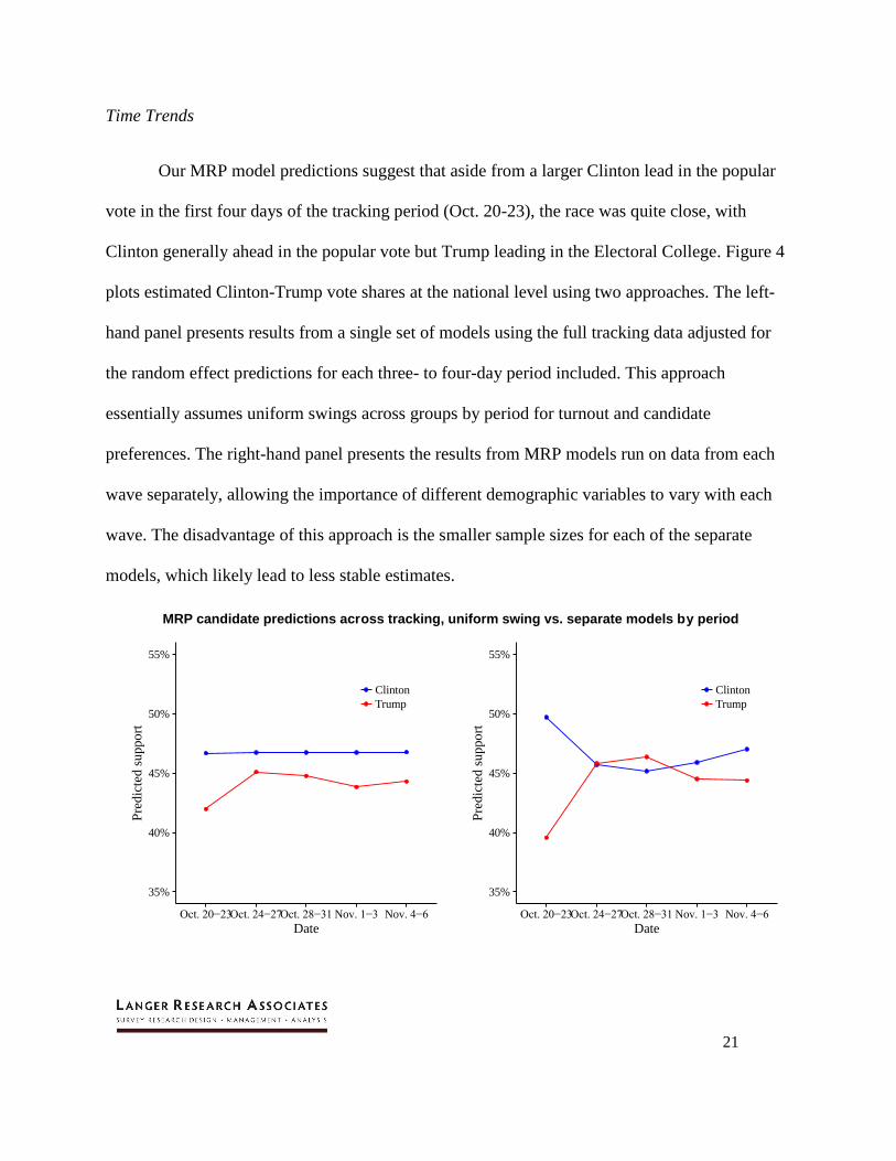
Our MRP model predictions suggest that aside from a larger Clinton lead in the popular

vote in the first four days of the tracking period (Oct. 20-23), the race was quite close, with

Clinton generally ahead in the popular vote but Trump leading in the Electoral College. Figure 4

plots estimated Clinton-Trump vote shares at the national level using two approaches. The left-

hand panel presents results from a single set of models using the full tracking data adjusted for

the random effect predictions for each three- to four-day period included. This approach

essentially assumes uniform swings across groups by period for turnout and candidate

preferences. The right-hand panel presents the results from MRP models run on data from each

wave separately, allowing the importance of different demographic variables to vary with each

wave. The disadvantage of this approach is the smaller sample sizes for each of the separate

models, which likely lead to less stable estimates.

MRP candidate predictions across tracking, uniform swing vs. separate models by period

35%

40%

45%

50%

55%

Oct. 20−23Oct. 24−27Oct. 28−31 Nov. 1−3 Nov. 4−6

Date

Pre

dic

ted s

up

po

rt

Clinton

Trump

35%

40%

45%

50%

55%

Oct. 20−23Oct. 24−27Oct. 28−31 Nov. 1−3 Nov. 4−6

Date

Pre

dic

ted s

up

po

rt

Clinton

Trump

22

Figure 4. MRP candidate support predictions across the tracking period. The left panel predictions

(“uniform swing”) are based on a single model including all of the tracking data with random effects for

each period. The right panel reports predictions for separate models for each period.

Both approaches suggest a large Clinton lead during the first four days, by five points

according to the “uniform swing” model and 10 points for the separate modeling approach. In

both cases, Clinton is predicted to win the Electoral College, though not overwhelmingly in the

uniform swing model (288-250). For both methods, the race narrows substantially after these

first four days, which followed the third presidential debate and a period in which Trump

underwent heavy criticism, including defections by GOP leaders, after the release of a videotape

in which he was heard crudely describing sexual advances toward a woman. Though Clinton

retained the support of about 46.7 percent of voters throughout the full course of tracking

according to the uniform swing approach, Trump came as close as 45.1 percent in the second

period (Oct. 24-27). In the separate modeling approach, Trump’s support exceeded Clinton’s

from Oct. 24-Oct. 31. With both approaches, Trump led Clinton in predicted Electoral College

votes during every period beyond the first four days. Notably, the narrowing of the contest at the

national level, and the flip in the Electoral College prediction, occurred prior to FBI Director

James Comey’s Oct. 28 letter to Congress about a renewal of the agency’s investigation into

Clinton’s email server.12

12 If the first four days are excluded from the analysis, MRP correctly predicts all 51 contests and RMSEs

are further reduced.

23

Subgroup Estimates

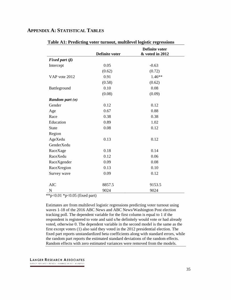
In terms of turnout, the subgroup-level variables that proved most predictive are

education, age, and (at some distance) race (see Table A1, column 2 in the Appendix). Variance

in turnout also is explained, but to lesser extents, by gender and state, and as well as by a number

of interactions between race and the other demographic variables. As far as fixed effects, the

VAP turnout in the respondent’s state in 2012 is highly predictive; while positive, the coefficient

associated with living in a battleground state does not reach conventional statistical significance.

Overall, these findings are consistent with research linking age and socioeconomic status with

turnout.

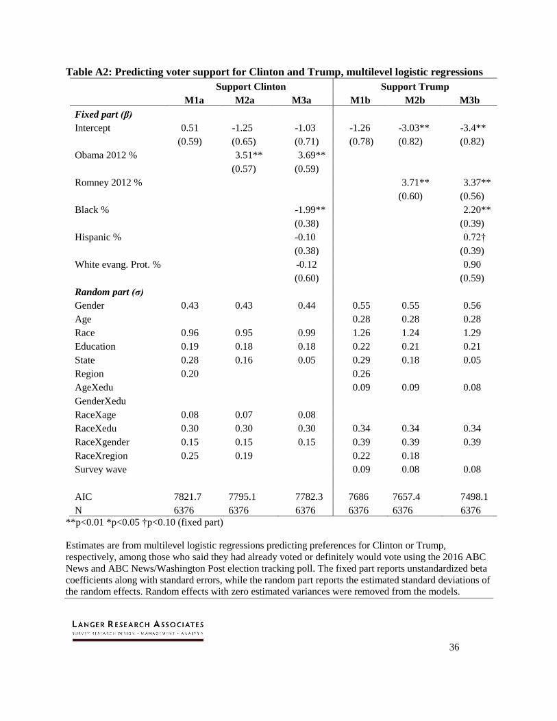
The variables that matter most for candidate preferences differ somewhat, but also

provide a clear picture of election dynamics (see Table A2, columns 3 and 6). Variance in

support for both Clinton and Trump is best explained by race/ethnicity, followed by gender, race

by education, race by gender and education on its own. Age is less important; it does not explain

support for Clinton and its impact on support for Trump is relatively minor compared with other

variables. Higher support for Clinton and lower support for Trump among younger generations is

more a function of higher levels of education and greater nonwhite shares among younger

Americans.

In terms of the fixed effects, Obama and Romney vote shares in the respondents’ states

are highly predictive, as is the proportion of each state’s residents who are African-American,

with higher shares related to lower support for Clinton and higher support for Trump, reflecting

the greater GOP lean of whites in states with higher percentages of African-American residents.

There’s a similar pattern for the Hispanic share of residents, though this variable only reaches

24

marginal levels of significance in the Trump support model. The influence of evangelical white

Protestants does not reach statistical significance in either model, though it just misses marginal

significance in positively predicting support for Trump.

To clarify the consequences of these patterns in turnout and support, it is possible to use

the poststratification dataset to generate subgroup level predictions of these outcomes. In doing

so, MRP provides a somewhat different story of the election dynamics than those portrayed by

the NEP national exit poll, differing most substantially by age group and whites by education.

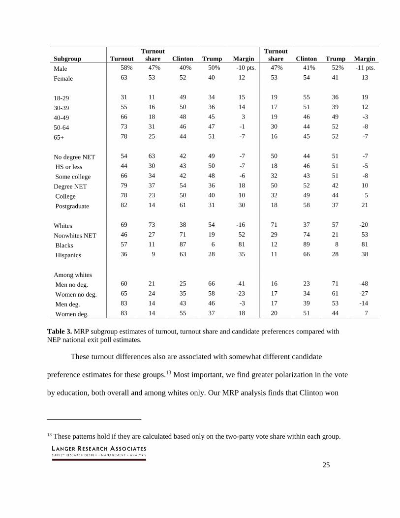
Table 3 compares MRP national estimates for subgroup-level turnout, turnout share and

candidate preferences with estimates from the national exit poll. In terms of turnout share, MRP

and the exit poll estimate the exact same shares of men and women (47-53 percent). By contrast,

our MRP analysis estimates turnout share among 18- to 29-year-olds at 11 percent, vs. 19

percent according to the exit poll, and MRP estimates seniors at 25 percent of voters, compared

with 16 percent in the exit poll. MRP also suggests that the electorate was much less well

educated; 63 percent of voters did not have a college degree according to our analysis, compared

with only half according to the exit poll. MRP puts the share of whites at 73 percent, compared

with 71 percent in the exit poll, with the 2-point difference coming equally from blacks and

Hispanics. Finally, differences emerge among whites by gender and education (degree vs. no

degree); while these four groups made up nearly equal shares of the electorate according to the

exit poll, whites without a college degree (both men and women) were a larger share of the

electorate according to our MRP analysis. The older, whiter and less well-educated electorate

from our MRP analysis is consistent with previous CPS-based estimates (Cohn 2016).

MRP Estimates NEP Exit Poll Estimates

25

Subgroup Turnout

Turnout

share Clinton Trump Margin

Turnout

share Clinton Trump Margin

Male 58% 47% 40% 50% -10 pts. 47% 41% 52% -11 pts.

Female 63 53 52 40 12 53 54 41 13

18-29 31 11 49 34 15 19 55 36 19

30-39 55 16 50 36 14 17 51 39 12

40-49 66 18 48 45 3 19 46 49 -3

50-64 73 31 46 47 -1 30 44 52 -8

65+ 78 25 44 51 -7 16 45 52 -7

No degree NET 54 63 42 49 -7 50 44 51 -7

HS or less 44 30 43 50 -7 18 46 51 -5

Some college 66 34 42 48 -6 32 43 51 -8

Degree NET 79 37 54 36 18 50 52 42 10

College 78 23 50 40 10 32 49 44 5

Postgraduate 82 14 61 31 30 18 58 37 21

Whites 69 73 38 54 -16 71 37 57 -20

Nonwhites NET 46 27 71 19 52 29 74 21 53

Blacks 57 11 87 6 81 12 89 8 81

Hispanics 36 9 63 28 35 11 66 28 38

Among whites

Men no deg. 60 21 25 66 -41 16 23 71 -48

Women no deg. 65 24 35 58 -23 17 34 61 -27

Men deg. 83 14 43 46 -3 17 39 53 -14

Women deg. 83 14 55 37 18 20 51 44 7

Table 3. MRP subgroup estimates of turnout, turnout share and candidate preferences compared with

NEP national exit poll estimates.

These turnout differences also are associated with somewhat different candidate

preference estimates for these groups.13 Most important, we find greater polarization in the vote

by education, both overall and among whites only. Our MRP analysis finds that Clinton won

13 These patterns hold if they are calculated based only on the two-party vote share within each group.

26

college graduates by 18 points, vs. only 10 points in the exit poll. Among whites, Trump won

both men and women without a college degree by slightly narrower margins according to MRP

relative to the exit poll, while Clinton pulled nearly evenly among white men with a college

degree (-3 vs. -14 Clinton-Trump) and was far ahead among white women with a college degree

(+18 vs. +7).

Put together, the exit poll suggests that whites were somewhat more pro-Trump than

MRP finds, going for the Republican candidate by 20 points, vs. by 16 points according to MRP.

Clinton’s margin of victory among blacks and Hispanics is similar in both approaches. Notably,

MRP suggests that Clinton won Hispanics by 35 points, close to the exit poll’s 38 points but

lower than some have argued using other data sources (Sanchez and Barreto 2016).

Our MRP estimates may be more accurate than the exit poll, which resorts to

observation-based adjustments to differential nonresponse by gender, race and age; weights

otherwise simply are used to align the data with actual vote results. Previous analyses have

suggested that these non-response adjustments are insufficient to compensate for higher exit poll

cooperation rates among more educated and younger voters (McDonald 2007; Cohn 2016). This

can lead to implausible estimates for turnout, particularly half of the electorate having college

degrees when only about three in 10 Americans have them. By forcing the data to “add up,” the

exit poll likely underestimated Clinton’s support among whites with college degrees and slightly

overestimated Trump’s support among less-educated whites.

27

V. PAST ELECTIONS

To assess the accuracy of the MRP approach across time, we conducted similar analyses

using ABC/Post tracking surveys for the 2000, 2004, 2008, and 2012 elections.14 While the

analyses differed slightly in the state-level variables15 included and the demographic interactions

that proved most predictive, the analyses essentially followed the methods described for the 2016

election.

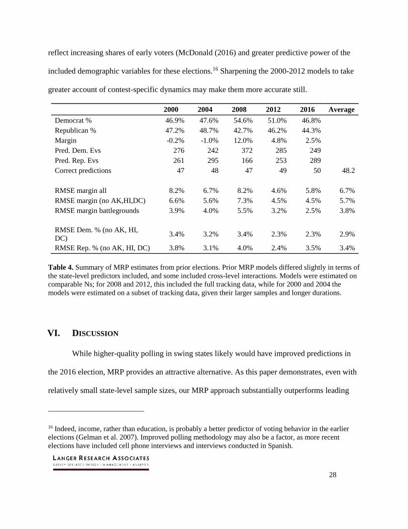
Table 4 summarizes the results for the last five presidential elections. On average, MRP

correctly predicts 48 of 51 contests; it misses the Electoral College and popular vote winner only

in the 2000 election. The average RMSE on the Democratic-Republican candidate margins

across elections in all 51 contests is 6.7 points, falling to 5.7 points when Alaska, Hawaii and

D.C. are excluded. For candidate percentages, the RMSE is 2.9-3.4 points on average, excluding

the idiosyncratic contests (Alaska, Hawaii and D.C.).

MRP correctly estimates an essentially tied race in 2000, but reverses the popular vote

and Electoral College winners. MRP slightly overestimates Obama in the popular vote and

Electoral College in 2008, while underestimating his Electoral College victory in 2012. The 2004

MRP slightly underestimates Bush’s popular vote and Electoral College victories. The 2012 and

2016 models are the most accurate, both in terms of correct state predictions and RMSE, with

2012 having the smallest errors. The greater accuracy of MRP in the last two elections may

14 The 2000 and 2004 tracking polls included more sample days and more respondents per day than the

latter tracking polls. For a clearer comparison, for these two elections a more limited number of tracking

days were analyzed to make for comparable sample sizes across elections. 15 For example, estimates of the proportion of evangelical white Protestants in each state were not

available for the first three elections.

28

reflect increasing shares of early voters (McDonald (2016) and greater predictive power of the

included demographic variables for these elections.16 Sharpening the 2000-2012 models to take

greater account of contest-specific dynamics may make them more accurate still.

2000 2004 2008 2012 2016 Average

Democrat % 46.9% 47.6% 54.6% 51.0% 46.8% Republican % 47.2% 48.7% 42.7% 46.2% 44.3% Margin -0.2% -1.0% 12.0% 4.8% 2.5% Pred. Dem. Evs 276 242 372 285 249 Pred. Rep. Evs 261 295 166 253 289 Correct predictions 47 48 47 49 50 48.2

RMSE margin all 8.2% 6.7% 8.2% 4.6% 5.8% 6.7%

RMSE margin (no AK,HI,DC) 6.6% 5.6% 7.3% 4.5% 4.5% 5.7%

RMSE margin battlegrounds 3.9% 4.0% 5.5% 3.2% 2.5% 3.8%

RMSE Dem. % (no AK, HI,

DC) 3.4% 3.2% 3.4% 2.3% 2.3% 2.9%

RMSE Rep. % (no AK, HI, DC) 3.8% 3.1% 4.0% 2.4% 3.5% 3.4%

Table 4. Summary of MRP estimates from prior elections. Prior MRP models differed slightly in terms of

the state-level predictors included, and some included cross-level interactions. Models were estimated on

comparable Ns; for 2008 and 2012, this included the full tracking data, while for 2000 and 2004 the

models were estimated on a subset of tracking data, given their larger samples and longer durations.

VI. DISCUSSION

While higher-quality polling in swing states likely would have improved predictions in

the 2016 election, MRP provides an attractive alternative. As this paper demonstrates, even with

relatively small state-level sample sizes, our MRP approach substantially outperforms leading

16 Indeed, income, rather than education, is probably a better predictor of voting behavior in the earlier

elections (Gelman et al. 2007). Improved polling methodology may also be a factor, as more recent

elections have included cell phone interviews and interviews conducted in Spanish.

29

polling aggregators in the 2016 election, and analyses of previous elections indicate the

robustness of the technique.

This performance is likely related to factors including the quality of the underlying data

and attributes specific to our approach. First, by using a single national-level survey, our MRP

estimates are based on data collected with the same methods across states, while state-level

surveys averaged by aggregators vary widely in methods and quality. To the extent that lower-

quality or poorly devised polling methods produce inaccurate estimates, the presumed canceling-

out benefits of aggregation can lead to biased and misleading results. Second, and relatedly, the

analysis reported here is based on one of the most methodologically sound probability-based

RDD surveys of its type in the country (Silver 2016). These data may present advantages over

non-probability data or voter registration lists; the latter suffer from sizable noncoverage and

noisy weighting variables.

MRP also offers an alternative to traditional survey weighting and likely voter modeling

that overcomes some of the challenges faced by standard survey weighting techniques (Gelman

2007) – either iterative proportional fitting, which does not guarantee precise subgroup sizes, or

cell weighting, which can be compromised by limited sample sizes. MRP is analogous in many

ways to cell weighting, without the troubles associated with zero- or small-n cells. In the analysis

presented here, the model estimates were poststratified on 10,200 cells, essentially a much finer-

grained weighting scheme than either rake or typical cell weighting.

Though it presents significant advantages, MRP is not a cure-all for challenges facing

pollsters. The greatest restriction is that MRP does not provide a single weight that can be used

30

for all variables in a survey; instead it requires each outcome of interest to be modeled

separately.

In another limitation, the relative accuracy of the approach in predicting recent state- and

national-level election outcomes is strongly related to the degree to which demographic variables

available for poststratification predict voting behavior. While such demographic variables have

been highly predictive in the past several elections, the future is unknown. To ensure continued

accuracy, researchers employing the technique need to adjust the demographic and state-level

predictors included in the model to the dynamics of any given election, based on exploratory data

analysis and other prior information.

Future research may lead to additional improvements in the accuracy of the MRP

approach employed here. Other strategies for estimating turnout (e.g., other deterministic

operationalizations, continuous turnout variables or CPS-based models) could enhance subgroup-

level turnout estimates. Future research also could examine whether and how to poststratify on

variables such as partisan identification or past vote (Wang et al. 2014; YouGov 2016), albeit

with an eye to the inherent risks of doing so. Finally, the analysis could be conducted using full

Bayesian methods, which would facilitate the calculation of uncertainty for the estimates.

For all its utility, MRP, in the application presented here, can only take us so far in

understanding the dynamics of an election. While, as we demonstrate, MRP can produce precise

state- and group-level turnout and candidate support predictions, it can only hint at how different

groups come to their choices. In this sense, MRP cannot replace more probing questions on

voters’ pre-political dispositions, policy preferences and views of candidate attributes that form

the substance of voter decision making. That said, we recognize the intense media and public

31

interest in discerning the likely winner of elections before they are held. If such predictions are to

remain a dominant element of our pre-election landscape, it is best that they be accurate.

32

REFERENCES

Bates, Douglas. 2005. “Fitting Linear Models in R Using the lme4 Package.” R News 5(1):27–

30.

Bialik, Carl and Harry Eten. 2016. “The Polls Missed Trump. We Asked Pollsters Why.”

Fivethirtyeight, Nov. 9. https://fivethirtyeight.com/features/the-polls-missed-trump-we-

asked-pollsters-why/

Cohn, Nate. 2016. “There are More White Voters than People Think. That’s Good News for

Trump.” The New York Times, June 9.

https://www.nytimes.com/2016/06/10/upshot/there-are-more-white-voters-than-people-

think-thats-good-news-for-trump.html

Cohn, Nate and Amanda Cox. 2016. “The Voting Habits of Americans Like You.” The New

York Times, June 10. https://www.nytimes.com/interactive/2016/06/10/upshot/voting-

habits-turnout-partisanship.html

Cohn, Nate, Josh Katz and Kevin Quealy. 2016. “Putting the Polling Miss of the 2016 Election

in Perspective.” The New York Times, Nov. 13.

https://www.nytimes.com/interactive/2016/11/13/upshot/putting-the-polling-miss-of-

2016-in-perspective.html

Eten, Harry. 2016. “Trump is Just a Normal Polling Error Behind Clinton.” Fivethirtyeight, Nov.

4. https://fivethirtyeight.com/features/trump-is-just-a-normal-polling-error-behind-

clinton/

Gelman, Andrew. 2007. “Struggles with survey weighting and regression modeling.” Statistical

Science 22(2): 153-164.

Gelman, Andrew and Jennifer Hill. 2007. Data Analysis Using Regression and Multilevel-

Hierarchical Models. Cambridge: Cambridge University Press.

Ghitza, Yair, and Andrew Gelman. 2013. "Deep interactions with MRP: Election turnout and

voting patterns among small electoral subgroups." American Journal of Political

Science 57(3): 762-776.

Lauderdale, Benjamin. 2016. “Election Model Methodology.” YouGov, Oct. 3.

https://today.yougov.com/news/2016/10/03/election-model-methodology/

Lax, Jeffrey R. and Justin H. Phillips. 2009a. “Gay Rights in the States: Public Opinion and

Policy Responsiveness.” American Political Science Review 103(3):367–86.

33

Lax, Jeffrey R. and Justin H. Phillips. 2009b. “How Should We Estimate Public Opinion in the

States?” American Journal of Political Science 53(1):107–21.

Linzer, Drew. 2016. “The forecasts were wrong. Trump won. What happened?” Daily Kos, Nov.

16. http://www.dailykos.com/stories/2016/11/16/1600472/-The-forecasts-were-wrong-

Trump-won-What-happened

McDonald, Michael P. 2007. “The True Electorate: A Cross-Validation of Voter Registration

Files and Election Survey Demographics. Public Opinion Quarterly 71 (4): 588-602.

McDonald, Michael P. 2016. “A Brief History of Early Voting.” Huffington Post, Sept. 28.

http://www.huffingtonpost.com/michael-p-mcdonald/a-brief-history-of-

early_b_12240120.html

Mercer, Andrew, Claudia Deane, and Kyley McGeeney. 2016. “Whey 2016 election polls

missed their mark.” Pew Research Center, Nov. 9. http://www.pewresearch.org/fact-

tank/2016/11/09/why-2016-election-polls-missed-their-mark/

Park, David K., Andrew Gelman and Joseph Bafumi. 2004. “Bayesian Multilevel Estimation

with Poststratification: State-Level Estimates from National Polls.” Political Analysis

12(4):375–85.

Pacheco, Julianna. 2011. “Using National Surveys to Measure State Public Opinion over Time:

A Guideline for Scholars and an Application.” State Politics and Policy Quarterly 11(4):

415–39.

Sanchez, Gabriel and Matt A. Barreto. 2016. “In record numbers, Latinos voted overwhelmingly

against Trump. We did the research.” Washington Post, Nov. 11.

https://www.washingtonpost.com/news/monkey-cage/wp/2016/11/11/in-record-numbers-

latinos-voted-overwhelmingly-against-trump-we-did-the-research/

Shephard, Steven. 2016. “GOP insiders: Polls don’t capture secret Trump vote.” Politico Oct. 28.

http://www.politico.com/story/2016/10/donald-trump-shy-voters-polls-gop-insiders-

230411

Silver, Nate. “Pollsters Probably Didn’t Talk to Enough White Voters without College Degrees.”

2016. Fivethirtyeight, Dec. 1. https://fivethirtyeight.com/features/pollsters-probably-

didnt-talk-to-enough-white-voters-without-college-degrees/

Silver, Nate. 2017. “The Real Story of 2016.” Fivethirtyeight, Jan. 19.

http://fivethirtyeight.com/features/the-real-story-of-2016/

34

Wang, Wei, David Rothschild, Sharad Goel, and Andrew Gelman. 2014. “Forecasting elections

with non-representative polls.” International Journal of Forecasting 31(3): 980-991.

Weigel, David. “State pollsters, pummeled by 2016, analyze what went wrong.” Washington

Post, Dec. 30. https://www.washingtonpost.com/news/post-politics/wp/2016/12/30/state-

pollsters-pummeled-by-2016-analyze-what-went-wrong/

35

APPENDIX A: STATISTICAL TABLES

Table A1: Predicting voter turnout, multilevel logistic regressions

Definite voter

Definite voter

& voted in 2012

Fixed part (β) Intercept 0.05 -0.63

(0.62) (0.72)

VAP vote 2012 0.91 1.46**

(0.58) (0.62)

Battleground 0.10 0.08

(0.08) (0.09)

Random part (σ) Gender 0.12 0.12

Age 0.67 0.88

Race 0.38 0.38

Education 0.89 1.02

State 0.08 0.12

Region AgeXedu 0.13 0.12

GenderXedu RaceXage 0.18 0.14

RaceXedu 0.12 0.06

RaceXgender 0.09 0.08

RaceXregion 0.13 0.10

Survey wave 0.09 0.12

AIC 8857.5 9153.5

N 9024 9024

**p<0.01 *p<0.05 (fixed part)

Estimates are from multilevel logistic regressions predicting voter turnout using

waves 1-18 of the 2016 ABC News and ABC News/Washington Post election

tracking poll. The dependent variable for the first column is equal to 1 if the

respondent is registered to vote and said s/he definitely would vote or had already

voted, otherwise 0. The dependent variable in the second model is the same as the

first except voters (1) also said they voted in the 2012 presidential election. The

fixed part reports unstandardized beta coefficients along with standard errors, while

the random part reports the estimated standard deviations of the random effects.

Random effects with zero estimated variances were removed from the models.

36

Table A2: Predicting voter support for Clinton and Trump, multilevel logistic regressions

Support Clinton Support Trump

M1a M2a M3a M1b M2b M3b

Fixed part (β) Intercept 0.51 -1.25 -1.03 -1.26 -3.03** -3.4**

(0.59) (0.65) (0.71) (0.78) (0.82) (0.82)

Obama 2012 % 3.51** 3.69**

(0.57) (0.59) Romney 2012 % 3.71** 3.37**

(0.60) (0.56)

Black % -1.99** 2.20**

(0.38) (0.39)

Hispanic % -0.10 0.72†

(0.38) (0.39)

White evang. Prot. % -0.12 0.90

(0.60) (0.59)

Random part (σ) Gender 0.43 0.43 0.44 0.55 0.55 0.56

Age 0.28 0.28 0.28

Race 0.96 0.95 0.99 1.26 1.24 1.29

Education 0.19 0.18 0.18 0.22 0.21 0.21

State 0.28 0.16 0.05 0.29 0.18 0.05

Region 0.20 0.26 AgeXedu 0.09 0.09 0.08

GenderXedu RaceXage 0.08 0.07 0.08 RaceXedu 0.30 0.30 0.30 0.34 0.34 0.34

RaceXgender 0.15 0.15 0.15 0.39 0.39 0.39

RaceXregion 0.25 0.19 0.22 0.18 Survey wave 0.09 0.08 0.08

AIC 7821.7 7795.1 7782.3 7686 7657.4 7498.1

N 6376 6376 6376 6376 6376 6376

**p<0.01 *p<0.05 †p<0.10 (fixed part)

Estimates are from multilevel logistic regressions predicting preferences for Clinton or Trump,

respectively, among those who said they had already voted or definitely would vote using the 2016 ABC

News and ABC News/Washington Post election tracking poll. The fixed part reports unstandardized beta

coefficients along with standard errors, while the random part reports the estimated standard deviations of

the random effects. Random effects with zero estimated variances were removed from the models.