predicting dengue importation into europe, using machine … · dengue or a destination node’s...

1

Predicting dengue importation into Europe, using machine learning and

model-agnostic methods.

Donald Salami1*, Carla Alexandra Sousa2*, Maria do Rosário Oliveira Martins2, César Capinha3*

1 Instituto de Higiene e Medicina Tropical, Universidade Nova de Lisboa, Global Public Health, Lisbon,

1349-008, Portugal

2 Instituto de Higiene e Medicina Tropical, Universidade Nova de Lisboa, Global Health and Tropical

Medicine, Lisbon, 1349-008, Portugal

3 Instituto de Geografia e Ordenamento do Território, Universidade de Lisboa, Centro de Estudos

Geográficos, Lisbon, 1600-276, Portugal

* Corresponding author

Email: [email protected] (DS)

[email protected] (CS)

[email protected] (CC)

. CC-BY-NC 4.0 International licenseIt is made available under a is the author/funder, who has granted medRxiv a license to display the preprint in perpetuity. was not certified by peer review)

(whichThe copyright holder for this preprint this version posted November 29, 2019. .https://doi.org/10.1101/19013383doi: medRxiv preprint

mailto:[email protected]



https://doi.org/10.1101/19013383

http://creativecommons.org/licenses/by-nc/4.0/

2

ABSTRACT

The geographical spread of dengue is a global public health concern. This is largely mediated by

the importation of dengue from endemic to non-endemic areas via the increasing connectivity of the

global air transport network. The dynamic nature and intrinsic heterogeneity of the air transport network

make it challenging to predict dengue importation.

Here, we explore the capabilities of state-of-the-art machine learning algorithms to predict

dengue importation. We trained four machine learning classifiers algorithms, using a 6-year historical

dengue importation data for 21 countries in Europe and connectivity indices mediating importation and

air transport network centrality measures. Predictive performance for the classifiers was evaluated using

the area under the receiving operating characteristic curve, sensitivity, and specificity measures. Finally,

we applied practical model-agnostic methods, to provide in-depth explanation of our optimal model’s

predictions on a global and local scale.

Our best performing model achieved high predictive accuracy, with an area under the receiver

operating characteristic score of 0.94 and a maximized sensitivity score of 0.88. The predictor variables

identified as most important were the source country’s dengue incidence rate, population size, and volume

of air passengers. Network centrality measures, describing the positioning of European countries within

the air travel network, were also influential to the predictions.

We demonstrated the high predictive performance of a machine learning model in predicting

dengue importation and the utility of the model-agnostic methods to offer a comprehensive understanding

of the reasons behind the predictions. Similar approaches can be utilized in the development of an

operational early warning surveillance system for dengue importation.



https://doi.org/10.1101/19013383


3

Introduction

The geographical spread of dengue fever is a global public health concern. This spread, particularly to

non-endemic areas, has been largely facilitated by an increase in global trade and human mobility 1-3. The

expansion and connectivity of the global air transport networks in recent years, has played a key role in

this spread 3. In Europe, where dengue is not endemic, the number of travel-related cases of dengue,

demonstrates how the air transport network has facilitated the spread of the disease. In the past decade,

the European region has reported a significant number of imported dengue cases from epidemic/endemic

tropical and subtropical countries 4. Sporadic autochthonous transmissions have also been triggered by

imported cases in areas with suitable environmental conditions and an established presence of the

mosquito vector 5. Recent examples include the autochthonous cases reported in France and Spain, which

were linked to having originated from an imported case 6.

The mitigation of the continuous spread of dengue in Europe lies in part in the ability to effectively

predict importation risk. However, a notable challenge in achieving this, is the complexity of global air

transport networks, due to the dynamic nature and heterogeneity underlying the connections 1,7,8. In recent

times a range of modelling approaches, from the field of social network analysis, have been applied to

understand the connection topology of the air transport network and their role in disease importation 9.

Unlike conventional statistical modelling approaches, these methods account for the co-dynamics of the

network structure and how they interact with other risk factors to mediate the importation of dengue 10-12.

Our previous work 13 integrates this modelling approach and offers a foundational understanding of the

importation patterns of dengue in Europe.

Conversely, an increasing number of studies are employing the use of machine learning

algorithms to develop robust predictive models for dengue 14,15. Machine learning algorithms are an

applied extension of artificial intelligence. These algorithms build a mathematical model base, to

automatically learn data patterns, adjust and perform inference, without explicit instructions 16. Several

studies have demonstrated the powerful predictive capabilities of machine learning models and their

superiority over conventional statistical methods 17-19. To this effect, some studies have applied them in

the development of predictive models for dengue incidence 14,20-22. A recent study by Chen et al 15, utilized

machine learning algorithms to develop a real-time model to forecast dengue in Singapore. Despite the

high predictive performance of machine learning algorithms, they are not widely popular in

epidemiological studies. This is likely to be in part because they are considered, to be “black-box” models

with low interpretability, due to their complex inner workings. We argue different, that though machine



https://doi.org/10.1101/19013383


4

learning models could fit complex relationships, several recent advancements have been made to aid the

interpretation of these models 23. To the best of our knowledge, machine learning algorithm has not been

applied in modelling the risk of dengue importation for Europe.

Here, we aim to apply machine learning algorithms to develop a predictive model for dengue importation

risk in Europe. To do so, we train a diverse set of machine learning algorithms, with historical data of

dengue importation into Europe, connectivity indices of factors potentially mediating importation risk and

centrality measures characterizing the air transport network. We then evaluate the predictive performance

of the different models on a hold-out dataset to determine an optimal model. And finally, we employ the

use of practical model-agnostic methods to interpret the optimal model’s predictions.

Methods

Dengue data

We obtained monthly data for imported cases of dengue in Europe, for 2010 – 2015, from the

European Centre for Disease Prevention and Control (ECDC) 24. Here, we utilized confirmed dengue

cases (as defined the European Union generic case definition for viral haemorrhagic fevers) with known

travel history 25. A total of 21 European Union/European Economic Area (EU/EEA) countries reported

data on imported dengue, from a total of 98 different source countries within the period of 2010 – 2015

(inclusive of zero reporting). The monthly level case counts were aggregated by country of infection (as

source country) and the reporting country in Europe (as destination country). We transform the absolute

count data into a binary response variable, that indicates whether there was an imported case of dengue

(1) or not (0) in a destination country, in a month.

Air passenger’s data

Comprehensive air passengers travel data for 2010 – 2015, was obtained from the International

Air Transport Association (IATA) 26. The data included true origin, connecting points and final-

destination airports for all routes in the world and their corresponding passengers’ volume. The data

contains over 11,996 airports in 229 different countries and their territorial dependencies. The passengers'

travel volume for each route worldwide was available at the country level and at a monthly timescale.

This data was used to construct a monthly passenger flow from all countries worldwide with a final-



https://doi.org/10.1101/19013383


5

destination in Europe (accounting for all connecting flights) for the period of 2010 – 2015. The data also

included the passengers' flow between European countries.

Connectivity indices between a source and destination country

Drawing on the underlining concept of spatial interaction modelling, that inflow between two

locations is a function of the attributes of the source and destination and their corresponding interaction 27.

Connectivity indices between a source country and a destination country in Europe were previously

developed 13, using different factors that potentially mediate dengue importation risk. The indices were

decomposed into components describing the source strength’ (the risk of dengue infection) and the

transport or importation potential (the connection between a source country and a potential destination

country in Europe). Source strength for all indices was modelled to represent the endemicity of dengue in

a source country. While transport and importation potential were modelled to characterize seasonal

dengue activity, incidence rates, geographical proximity, epidemic vulnerability, air passenger volume,

population size and wealth of a source country as mediating risk factors. The connectivity indices and

their descriptions are listed in Table 1.

Centrality measures of the air transport network

Using the monthly air passenger’s data, we constructed a weighted directed network. The

network for each month was denoted by 𝐺𝑚 = (𝑉, 𝐸), where 𝑉𝐺 is a set containing all the nodes (or

vertices), while 𝐸𝐺 contains all the edges, with 𝑚 indicating the month (m = 1, 2, 3… 72, covering the

years of 2010 – 2015). Nodes represented all countries worldwide, while edges represent the flow of

passengers from a source country to a destination country in Europe. Four different centrality measures

were used to analyse the network and quantify the capacity of a source node to influence transportation of

dengue or a destination node’s propensity to receive an imported case of dengue, by virtue of their

connection topology within the network. Centrality measures and their descriptions are listed in Table 1.

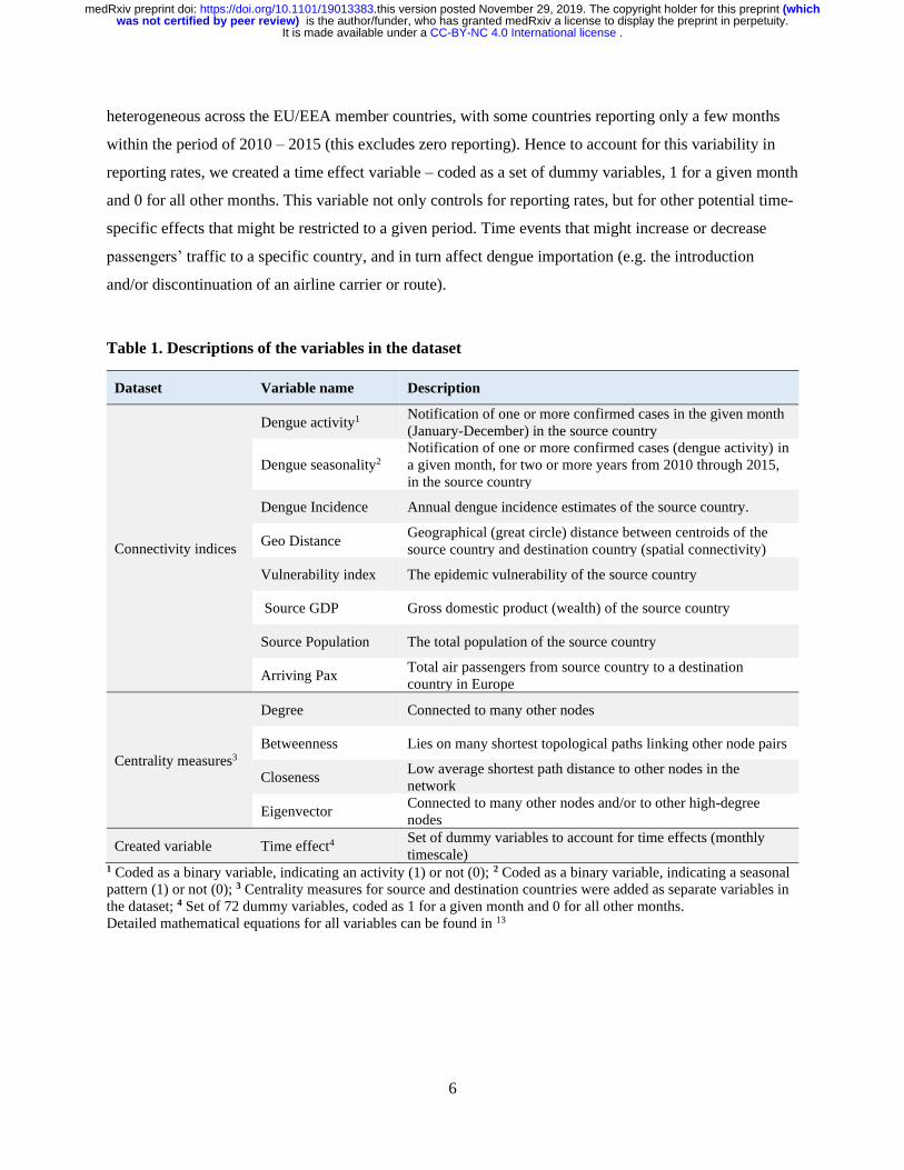
Feature (variable) engineering

One fundamental step in building machine learning models is the process of feature engineering,

i.e. using domain-specific knowledge to create new features (i.e. variables) or transform and encode

existing original data into a more informative format 28,29. For this analysis, we created an additional

variable based on our a priori knowledge of the data. The reporting rate for dengue data was



https://doi.org/10.1101/19013383


6

heterogeneous across the EU/EEA member countries, with some countries reporting only a few months

within the period of 2010 – 2015 (this excludes zero reporting). Hence to account for this variability in

reporting rates, we created a time effect variable – coded as a set of dummy variables, 1 for a given month

and 0 for all other months. This variable not only controls for reporting rates, but for other potential time-

specific effects that might be restricted to a given period. Time events that might increase or decrease

passengers’ traffic to a specific country, and in turn affect dengue importation (e.g. the introduction

and/or discontinuation of an airline carrier or route).

Table 1. Descriptions of the variables in the dataset

Dataset Variable name Description

Connectivity indices

Dengue activity1 Notification of one or more confirmed cases in the given month

(January-December) in the source country

Dengue seasonality2

Notification of one or more confirmed cases (dengue activity) in

a given month, for two or more years from 2010 through 2015,

in the source country

Dengue Incidence Annual dengue incidence estimates of the source country.

Geo Distance Geographical (great circle) distance between centroids of the

source country and destination country (spatial connectivity)

Vulnerability index The epidemic vulnerability of the source country

Source GDP Gross domestic product (wealth) of the source country

Source Population The total population of the source country

Arriving Pax Total air passengers from source country to a destination

country in Europe

Centrality measures3

Degree Connected to many other nodes

Betweenness Lies on many shortest topological paths linking other node pairs

Closeness Low average shortest path distance to other nodes in the

network

Eigenvector Connected to many other nodes and/or to other high-degree

nodes

Created variable Time effect4 Set of dummy variables to account for time effects (monthly

timescale) 1 Coded as a binary variable, indicating an activity (1) or not (0); 2 Coded as a binary variable, indicating a seasonal

pattern (1) or not (0); 3 Centrality measures for source and destination countries were added as separate variables in

the dataset; 4 Set of 72 dummy variables, coded as 1 for a given month and 0 for all other months.

Detailed mathematical equations for all variables can be found in 13



https://doi.org/10.1101/19013383


7

Data pre-processing and splitting

The dataset used to build our machine learning models consists of the connectivity indices and

centrality measures of the air transport network. The single unit of analysis is a source-destination country

pair, at a monthly timescale, and a binary response variable coded to indicate an imported dengue case (1)

or not (0).

Prior to model training, we performed the following pre-processing analyses to the full dataset.

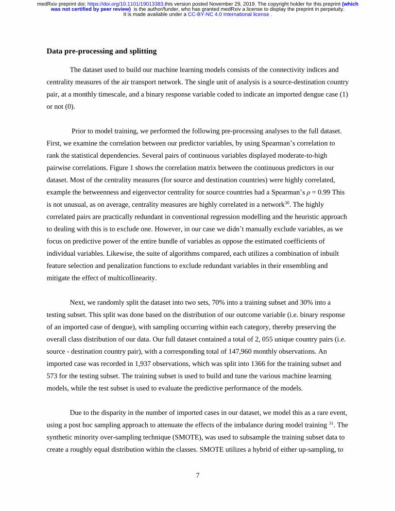
First, we examine the correlation between our predictor variables, by using Spearman’s correlation to

rank the statistical dependencies. Several pairs of continuous variables displayed moderate-to-high

pairwise correlations. Figure 1 shows the correlation matrix between the continuous predictors in our

dataset. Most of the centrality measures (for source and destination countries) were highly correlated,

example the betweenness and eigenvector centrality for source countries had a Spearman’s ρ = 0.99 This

is not unusual, as on average, centrality measures are highly correlated in a network30. The highly

correlated pairs are practically redundant in conventional regression modelling and the heuristic approach

to dealing with this is to exclude one. However, in our case we didn’t manually exclude variables, as we

focus on predictive power of the entire bundle of variables as oppose the estimated coefficients of

individual variables. Likewise, the suite of algorithms compared, each utilizes a combination of inbuilt

feature selection and penalization functions to exclude redundant variables in their ensembling and

mitigate the effect of multicollinearity.

Next, we randomly split the dataset into two sets, 70% into a training subset and 30% into a

testing subset. This split was done based on the distribution of our outcome variable (i.e. binary response

of an imported case of dengue), with sampling occurring within each category, thereby preserving the

overall class distribution of our data. Our full dataset contained a total of 2, 055 unique country pairs (i.e.

source - destination country pair), with a corresponding total of 147,960 monthly observations. An

imported case was recorded in 1,937 observations, which was split into 1366 for the training subset and

573 for the testing subset. The training subset is used to build and tune the various machine learning

models, while the test subset is used to evaluate the predictive performance of the models.

Due to the disparity in the number of imported cases in our dataset, we model this as a rare event,

using a post hoc sampling approach to attenuate the effects of the imbalance during model training 31. The

synthetic minority over-sampling technique (SMOTE), was used to subsample the training subset data to

create a roughly equal distribution within the classes. SMOTE utilizes a hybrid of either up-sampling, to



https://doi.org/10.1101/19013383


8

synthesize new data points in the minority class or down-sampling, to down-size the majority class 32. Our

training dataset was balanced to a 3:4 ratio of an imported case to no imported case. The testing subset

was maintained to reflect the original imbalance as a quality assurance of the predictive model

performance. Lastly, before training, we apply a data transformation on all continuous variables in the

dataset, by centring and scaling them. This transformation ensures that the variables have a zero mean and

a common standard deviation of one, thereby improving normality and the numerical stability of the

model calculations 29.

Figure 1. Spearman correlation matrix of continuous variables. Correlation is computed from the full dataset

and coloured according to magnitude. Red colours indicate strong positive correlations, blue indicates strong

negative correlations, and yellow implies no empirical relationship between the variables.

Model selection

Our training model is a classification-based model, to predict the probability that a case of dengue

is imported into a country in Europe. There are several classification techniques (or classifiers) employed

in machine learning models. The choice of the suite of algorithms we tested, was a trade-off between,

meta-algorithm that fits our classification problem and those with built-in feature selection. Other



https://doi.org/10.1101/19013383


9

algorithmic and systematic features that were considered include regularization (to handle the effects of

multicollinearity), hyperparameter optimization (model tuning capabilities), and efficient computation

time. To build our predictive model, we compare four widely used classifiers algorithms in machine

learning, as listed below:

Partial least squares (pls) implements a supervised version of principal component analysis, using a

dimension reduction technique. This technique first summarizes the original variables into a few new

variables called principal components (PCs), as supervised by their relationship to the outcome variable.

These components are then used to fit a linear regression model 33. For classification problems, the partial

least squares discriminant analysis variant is fitted. This method has an embedded feature selection and

regularization 34.

Lasso and elastic-net regularized generalized linear models (glmnet) implement a logistic generalized

linear model via penalized maximum likelihood. The addition of a penalty shrinks the coefficients of the

less contributive variables toward zero (L2 ridge penalty) or absolute zero (L1-Lasso penalty)35. The

glmnet implements a combination of both L1 & L2 penalties (otherwise called elastic net penalty), for its

regularization and simultaneous feature selection.

Random forest (randomForest) is a bootstrap aggregated (or bagged) decision tree-based ensemble

technique. The algorithm constructs multiple decision trees by repeat resampling of the training dataset

and outputs the mode of the classes as a consensus prediction. The trees are created independently from a

random vector distribution; hence each individual tree is heterogeneous with high variance and casts a

unit vote for the most popular class 36. By averaging several decision trees, it intuitively avoids overfitting

and performs an embedded feature selection.

Extreme gradient boosting (xgboost) implementation of a gradient boosted decision trees ensemble

technique. The gradient boosting framework iteratively refines its model, to create a strong classifier by

combining multiple weak classifiers in a stage-wise manner to minimize the loss function 37,38. The

xgboost algorithm is a commonly preferred classifier, because it utilizes parallelization and distributed

computation for implementation, thereby ensuring high efficiency in computation time and resources 39.

Model tuning and validation

Machine learning models can be prone to overfitting, to mitigate this we implemented a model

building approach that encompasses model tuning and repeated evaluation during training. We use a

methodological resampling technique of the training dataset, i.e. five repeats of 10-fold cross-validation



https://doi.org/10.1101/19013383


10

(CV). The 10-fold CV randomly partitions the training dataset into 10 sets of roughly equal size, one set

retained, and the others used to fit a model. The retained set is used to estimate model performance. The

first set is then returned to the training set and the procedure iterated until each set has been used for

validation. This whole process is repeated five times before results are aggregated and summarized. This

procedure automatically chooses tuning parameters associated with optimal model performance.

Candidate models were evaluated using the following performance metrics: area under the

receiving operating characteristic curve (AUC), sensitivity (true positive rate), and specificity (false

positive rate). Our final candidate model was selected based on the receiving operating characteristic

curve (ROC) threshold, which maximizes the trade-off between sensitivity and specificity 40. The ROC

curve evaluates the class probabilities across a continuum of thresholds, with an arbitrary (algorithmically

set) “optimal” cut point for determining what percentage of probability is accepted in classifying an

imported case of dengue.

Model interpretability

We employ the use of recent model-agnostic tools with both global and local scale interpretability

functions to our optimal model 23. Global interpretation helps to understand the modelled relationship and

distribution of the predicted target outcome (i.e. dengue importation) based on the input variables, while

local interpretation zooms in, to help understand model predictions for a single instance (i.e. a single unit

of observation or analysis).

We obtained global interpretations of our final candidate model through the following, variable

importance and partial dependence plots 41,42. Variable importance measures the contribution of each

input variable, by calculating the increase in the model’s prediction error after permuting the variable 43.

While the Partial dependence plots (PDP) are graphical renderings of the prediction function that helps

visualize the relationship between the variables and predicted outcome 44-46. The relative importance of

each variable is normalized to have a maximum value of 100, with higher scores indicating the most

influential variable. We note that it may not be feasible to explore in detail the relationship of all variables

in our model. Hence, we set an arbitrary cut off on the variable importance measures at a value >50, to

determine a subset of variables to focus on.

Local interpretation of our model was implemented via the use of local surrogate models,

otherwise called- Local interpretable model-agnostic explanations (LIME) 23,47,48. The underlining



https://doi.org/10.1101/19013383


11

assumption of LIME is that complex black box models are linear on a local scale, hence a simple

(surrogate) model can be fitted for an individual observation that mimics the behaviour of the global

model at this locality. The simple model and its variable weights are then used to explain the individual

predictions locally. To demonstrate the LIME technique, we selected 10 single observations from our

initial testing subset. These observations were sampled methodologically to include both classes (i.e.

imported case [1] or not [0]) and representative of countries with a high and low frequency of dengue

importation. We set the number of variables to best describe the predicted outcome, as the 5 most

influential. The resulting weights for these variables are plotted to explain the local behaviour of the

model. The plots delineate if a variable supports or contradicts the predicted probability of an imported

case of dengue (detailed vignette for the LIME techniques can be found here 49,50.

Statistical software

All statistical analyses were performed with R Programming Language version 3.6.1 51. For

uniformity in our model build, we utilized the Classification and regression training (caret) R package,

this is an interface to a vast amount of available machine learning algorithms 52. caret streamlines the

process of building and validating predictive models by using a set of intuitive call functions. Supporting

packages for specific functions includes: pls 34, glmnet 35, randomForest 53, xgboost 54, plyr 55, doSNOW

56, DMwR 57, pROC 58, pdp 46, iml 59, lime 60 and their various dependencies.

Results

Model prediction performance

We compared the prediction performance of the different classifiers’ algorithms, in their ability to

predict an imported case of dengue. Models were evaluated with the testing dataset, utilizing the area

under the receiver operating characteristic curve (AUC) as the quantitative measure for performance

comparisons. All four models performed comparably well, with AUC scores above 0.80 (Table 2). AUC

score using pls was 0.88 (95% CI, 0.86 to 0.90); glmnet was 0.89 (95% CI, 0.87 to 0.91); randomForest

was 0.97 (95% CI, 0.96 to 0.98); and xgboost was 0.97 (95% CI, 0.96 to 0.98). Performance metrics for

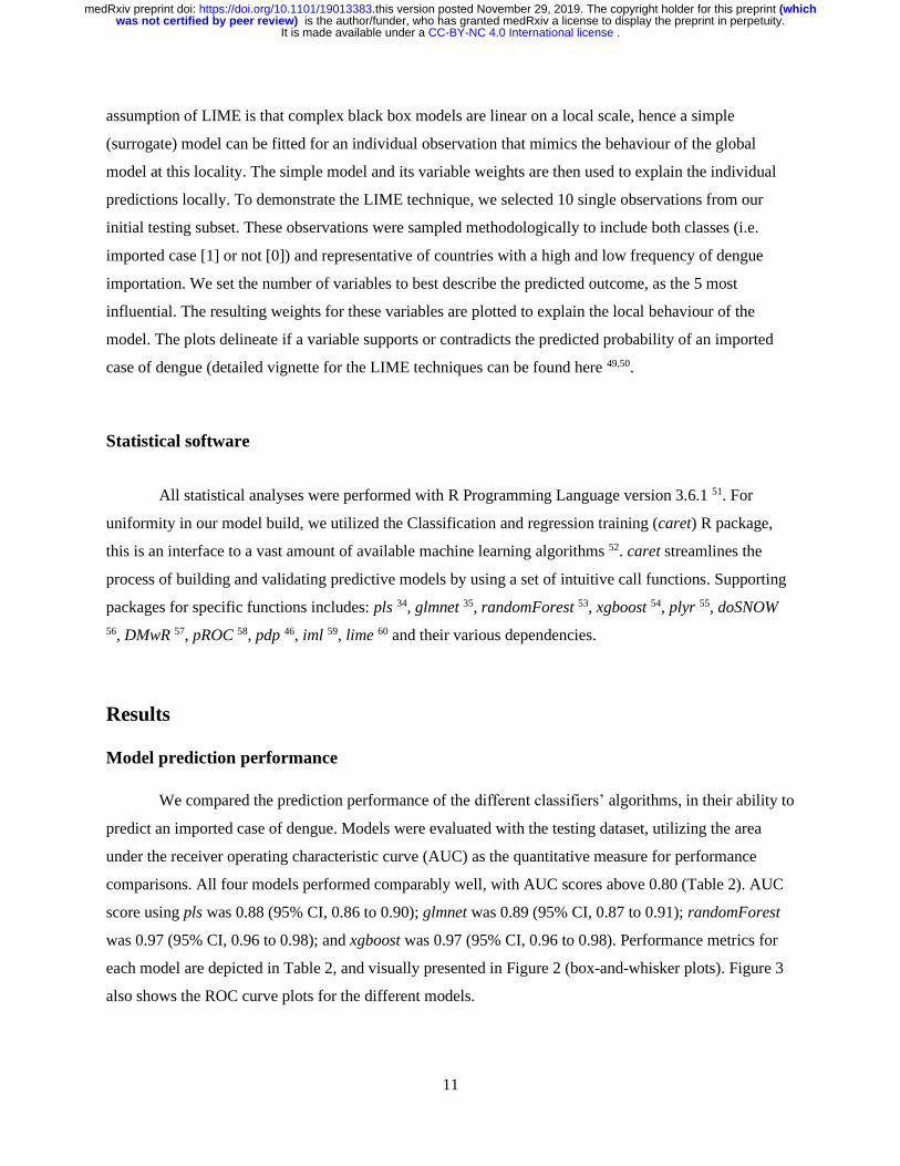
each model are depicted in Table 2, and visually presented in Figure 2 (box-and-whisker plots). Figure 3

also shows the ROC curve plots for the different models.



https://doi.org/10.1101/19013383


12

Table 2. Comparison of the prediction performance of the different models

Model AUC (95% CI) Sensitivity Specificity

pls 0.88 (0.86 - 0.89) 0.75 0.84

glmnet 0.89 (0.87 - 0.90) 0.77 0.84

randomForest 0.94 (0.93 - 0.95) 0.79 0.92

xgboost 0.94 (0.94 - 0.95) 0.79 0.93

AUC = area under the ROC curve; Sensitivity = rate of an imported case predicted correctly (true positive rate);

Specificity = rate that non-imported cases are predicted correctly (false positive rate).

Figure 2. Box-and-whisker plots for prediction performance of the different models. ROC = area under the

ROC curve; Sens = Sensitivity (true positive rate); Spec = Specificity (false positive rate).



https://doi.org/10.1101/19013383


13

Figure 3. Comparison of the receiver operator characteristic (ROC) curve for the different models. Curves

characterize the trade-offs between the sensitivity (true positive rate) and specificity (false positive rate). The y-axis

= sensitivity and the x-axis = 1 minus specificity.

The AUC score indicates that predictions from the randomForest and xgboost models were better

fitted to the dataset, outperforming the pls and glmnet models (with the pls being the least fitted). The

randomForest and xgboost models had similar performance across the metrics with nearly negligible

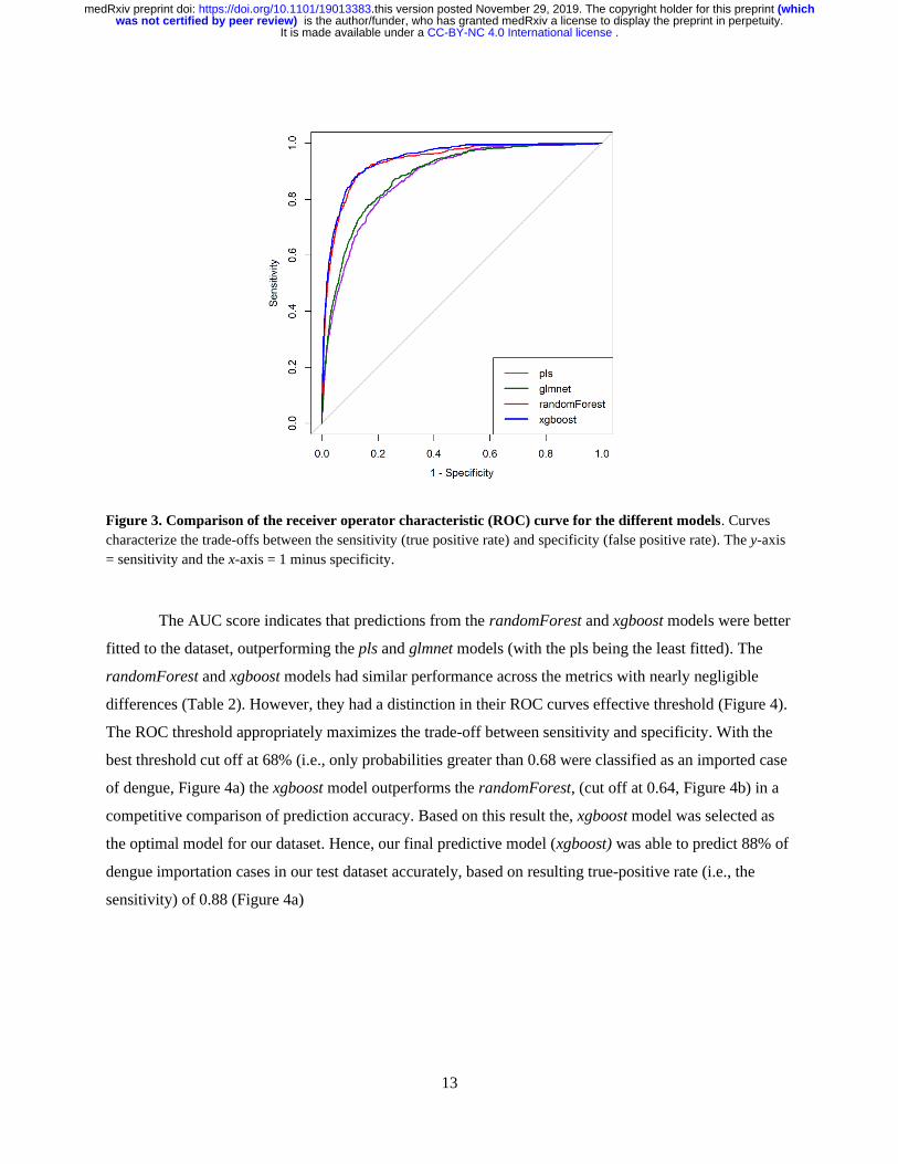
differences (Table 2). However, they had a distinction in their ROC curves effective threshold (Figure 4).

The ROC threshold appropriately maximizes the trade-off between sensitivity and specificity. With the

best threshold cut off at 68% (i.e., only probabilities greater than 0.68 were classified as an imported case

of dengue, Figure 4a) the xgboost model outperforms the randomForest, (cut off at 0.64, Figure 4b) in a

competitive comparison of prediction accuracy. Based on this result the, xgboost model was selected as

the optimal model for our dataset. Hence, our final predictive model (xgboost) was able to predict 88% of

dengue importation cases in our test dataset accurately, based on resulting true-positive rate (i.e., the

sensitivity) of 0.88 (Figure 4a)



https://doi.org/10.1101/19013383


14

Figure 4. Comparison of the receiver operator characteristic (ROC) curves for extreme gradient boosting and

random forest models. The dot on both plots indicates the value corresponding to the “best” cut-off point threshold

for each model that appropriately maximizes the trade-off between sensitivity and specificity. The numbers in

parentheses are (specificity, sensitivity). Extreme gradient boosting (a) cut-off was at 68% (i.e., probabilities greater

than 0.68 are classified as an imported case of dengue), delivering a specificity of 0.883, sensitivity of 0.880, while

random forest (b) cut-off was at 64%.

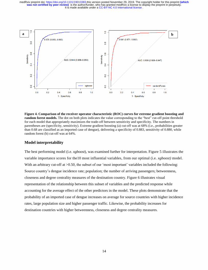
Model interpretability

The best performing model (i.e. xgboost), was examined further for interpretation. Figure 5 illustrates the

variable importance scores for the10 most influential variables, from our optimal (i.e. xgboost) model.

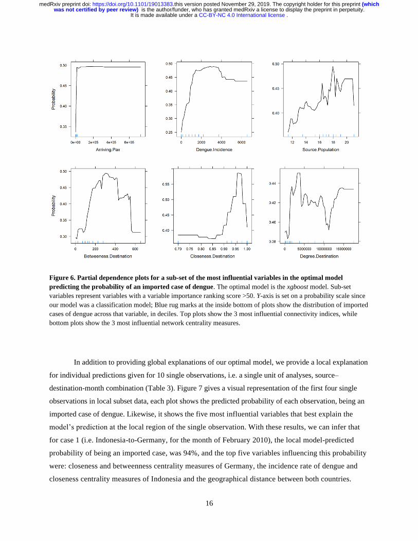
With an arbitrary cut-off at >0.50, the subset of our ‘most important’ variables included the following:

Source country’s dengue incidence rate; population; the number of arriving passengers; betweenness,

closeness and degree centrality measures of the destination country. Figure 6 illustrates visual

representation of the relationship between this subset of variables and the predicted response while

accounting for the average effect of the other predictors in the model. These plots demonstrate that the

probability of an imported case of dengue increases on average for source countries with higher incidence

rates, large population size and higher passenger traffic. Likewise, the probability increases for

destination countries with higher betweenness, closeness and degree centrality measures.

a b



https://doi.org/10.1101/19013383


15

Figure 5. Variable importance plots. Top 10 most influential variables from the extreme gradient boosting model.

The relative importance of each variable is normalized to have a maximum value of 100, with higher scores

indicating the most influential variable.



https://doi.org/10.1101/19013383


16

Figure 6. Partial dependence plots for a sub-set of the most influential variables in the optimal model

predicting the probability of an imported case of dengue. The optimal model is the xgboost model. Sub-set

variables represent variables with a variable importance ranking score >50. Y-axis is set on a probability scale since

our model was a classification model; Blue rug marks at the inside bottom of plots show the distribution of imported

cases of dengue across that variable, in deciles. Top plots show the 3 most influential connectivity indices, while

bottom plots show the 3 most influential network centrality measures.

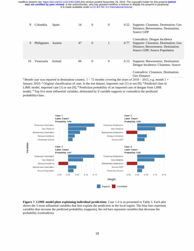
In addition to providing global explanations of our optimal model, we provide a local explanation

for individual predictions given for 10 single observations, i.e. a single unit of analyses, source–

destination-month combination (Table 3). Figure 7 gives a visual representation of the first four single

observations in local subset data, each plot shows the predicted probability of each observation, being an

imported case of dengue. Likewise, it shows the five most influential variables that best explain the

model’s prediction at the local region of the single observation. With these results, we can infer that

for case 1 (i.e. Indonesia-to-Germany, for the month of February 2010), the local model-predicted

probability of being an imported case, was 94%, and the top five variables influencing this probability

were: closeness and betweenness centrality measures of Germany, the incidence rate of dengue and

closeness centrality measures of Indonesia and the geographical distance between both countries.



https://doi.org/10.1101/19013383


17

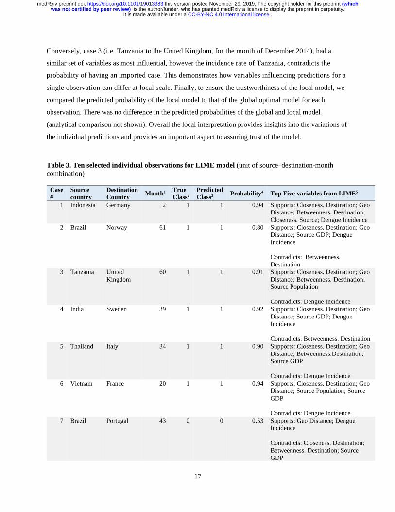
Conversely, case 3 (i.e. Tanzania to the United Kingdom, for the month of December 2014), had a

similar set of variables as most influential, however the incidence rate of Tanzania, contradicts the

probability of having an imported case. This demonstrates how variables influencing predictions for a

single observation can differ at local scale. Finally, to ensure the trustworthiness of the local model, we

compared the predicted probability of the local model to that of the global optimal model for each

observation. There was no difference in the predicted probabilities of the global and local model

(analytical comparison not shown). Overall the local interpretation provides insights into the variations of

the individual predictions and provides an important aspect to assuring trust of the model.

Table 3. Ten selected individual observations for LIME model (unit of source–destination-month

combination)

Case

#

Source

country

Destination

Country Month1

True

Class2

Predicted

Class3 Probability4 Top Five variables from LIME5

1 Indonesia Germany 2 1 1 0.94 Supports: Closeness. Destination; Geo

Distance; Betweenness. Destination;

Closeness. Source; Dengue Incidence

2 Brazil Norway 61 1 1 0.80 Supports: Closeness. Destination; Geo

Distance; Source GDP; Dengue

Incidence

Contradicts: Betweenness.

Destination

3 Tanzania United

Kingdom

60 1 1 0.91 Supports: Closeness. Destination; Geo


Source Population

Contradicts: Dengue Incidence

4 India Sweden 39 1 1 0.92 Supports: Closeness. Destination; Geo

Distance; Source GDP; Dengue

Incidence

Contradicts: Betweenness. Destination

5 Thailand Italy 34 1 1 0.90 Supports: Closeness. Destination; Geo

Distance; Betweenness.Destination;

Source GDP


6 Vietnam France 20 1 1 0.94 Supports: Closeness. Destination; Geo

Distance; Source Population; Source

GDP


7 Brazil Portugal 43 0 0 0.53 Supports: Geo Distance; Dengue

Incidence

Contradicts: Closeness. Destination;

Betweenness. Destination; Source

GDP



https://doi.org/10.1101/19013383


18

1 Month case was reported in destination country, 1 – 72 months covering the years of 2010 – 2015, e.g. month 1 =

January 2010; 2 Original classification of case, in the test dataset, imported case [1] or not [0]; 3 Predicted class in

LIME model, imported case [1] or not [0]; 4 Prediction probability of an imported case of dengue from LIME

model; 5 Top five most influential variables, delineated by if variable supports or contradicts the predicted

probability/class.

Figure 7. LIME model plots explaining individual predictions. Case 1-4 is as presented in Table 3. Each plot

shows the 5 most influential variables that best explain the prediction in the local region. The blue bars represent

variables that increase the predicted probability (supports), the red bars represent variables that decrease the

probability (contradicts).

8 Columbia Spain 14 0 0 0.52 Supports: Closeness. Destination; Geo


Source GDP


9 Philippines Austria 47 0 1 0.77 Supports: Closeness. Destination; Geo


Source GDP; Source Population

10 Venezuela Ireland 66 0 0 0.13 Supports: Betweenness. Destination;

Dengue Incidence; Closeness. Source

Contradicts: Closeness. Destination;

Geo Distance



https://doi.org/10.1101/19013383


19

Discussion

Our study demonstrates the use of machine learning modelling approach to predict the probability

of having an imported case of dengue in Europe. Using historical dengue importation data, we trained and

evaluated four machine learning classifiers algorithms, to develop an optimal predictive model. Our best-

performing model was the extreme gradient boosting model with an AUC score of 0.94, sensitivity of

0.79 and specificity of 0.93. Our choice of best performing model was not just based on the AUC results,

as this score does not necessarily guarantee the best classifier. Given that our prediction target is the

probability of having an imported case of dengue, we expected our final model performs better in

capturing the true cases (i.e. maximizing sensitivity) and limits the false negatives. This was achieved by

the effective probability threshold of the ROC curve, which offered a trade-off between sensitivity and

specificity. Utilizing this we were able to maximize the sensitivity of our optimal model, to predict

correctly the probability of an imported case of dengue with an 88% accuracy rate. As a first attempt to

train a machine learning model for dengue importation in Europe, we can safely state that our model

provides a benchmarking result for predictive performance. Given this predictive performance, our model

holds great potential as a forecasting tool which can markedly improve dengue surveillance in Europe.

A limitation of other previous machine learning models is that they deliver high predictive

accuracy without explaining why certain predictions are made 14,61. In this paper, we posit for both

accuracy and interpretability of our final model. We focus on demonstrating the practical explanation of

our model predictions using recent model-agnostic approaches 23. Our model included 17 predictor

variables, which broadly captures the importation risk factors (as presented by the connectivity indices)

and the influence of the air transport network (i.e. the centrality measures). These variables were chosen

to reflect the factors known or hypothesized to be relevant to the importation dynamics. So firstly, we

provided an overall quantification of the relationship between our model variables and the predicted

outcome, by ranking them in terms of their importance. With a further exploratory analysis (via the PDPs

visualizations) concentrating on a sub-set of the most influential variables. On average our model

predicted a higher probability of an imported case of dengue, from a source country with high dengue

incidence rates, large population and high air passenger volume. These findings support a priori

expectation for these factors to increase the importation risk of dengue and are consistent with other

studies 12,13,62. In addition, it predicts a higher probability of an imported case for destination countries

with high connectivity within the network (as measured by degree centrality), with a putative connection

hub to other countries (betweenness centrality) and connects to other countries in a relatively short



https://doi.org/10.1101/19013383


20

amount of time (closeness centrality). Intuitively, this is expected, given that the network centrality of the

destination country was modelled to act as a proxy for a country’s propensity to receive an imported case.

Hence, destination countries with higher connectivity within the network have an increased risk of

importation. These findings are similar to other previous studies that characterize the role of the air

transport network structure in mediating epidemic spread 10,11 and collaborates the results of our previous

work 13.

The above explanations capture the relative contribution of the input variables in predicting the

importation of dengue at an aggregated level for Europe. However, the risk probabilities will differ at the

country level due to changes in the dynamic attributes of the different country pairs. For example, the

dengue activity or seasonality in a source country can vary relative to time (oblivious to high or low

incidence rates). Hence, it will be expected that importation risk based on seasonality will have temporal

differences between source countries. Also, the volume of air passengers between country pairs are

heterogeneous, which can be largely determined by different monthly traffic flows. Also, the topological

profile of the air travel network will differ across countries with changes in passenger volume. These

heterogeneities may affect the prediction of dengue importation at the country level, with certain variables

supporting or contradicting depending on the country pairs in consideration. Using the local interpretable

model-agnostic explanations, we were able to asses which variables are most influential on the

predictions at a temporal and country level. As illustrated from the examples in Table 3, the probability

risk prediction for different country pairs was supported or contradicted by different variable

combinations at discrete points in time. For example, the predicted probability of a case of dengue from

Indonesia (case 1 in Table 3) and Tanzania (case 3 in Table 3), were similar, but vary in the risk factors

mediating this prediction. The lower dengue incidence rates in Tanzania (relative to Indonesia), did not

support the probability of an imported case, however other variables pose a risk of dengue hence the

prediction. Overall the local explanations provide insights into the heterogeneities of variables influencing

importation at the different country pairing levels (i.e. a source and destination country pair). This local-

level explanation can be useful in profiling a destination country importation risk from a specific source

country or region; in a similar manner to the route-level risk assessment discussed by Gardner et al 10.

This type of information can help guide the implementation of targeted surveillance which effective

appropriates resources for European countries at higher risk of dengue importation.

Overall our work demonstrates the utility of machine learning algorithms in the development of a

predictive model for the importation of dengue in Europe; with major steps towards improving the

understanding behind the model predictions. However, there are some limitations to this work, that is



https://doi.org/10.1101/19013383


21

worth noting for improvement in future research: (1) Dengue incidence rate for source countries was

aggregated at a yearly scale, due to paucity of surveillance data at a similar scale to dengue case data (i.e.

monthly). This may have overestimated or underestimated the actual effect of incidence and potentially

impact the predicted risk probability from a source country. Our approach compensated for this limitation

by the inclusion of the dengue activity and seasonality variables. Even though this does not necessarily

capture the variability of a finer scale but serves as a proxy. (2) We only evaluated our prediction as a

binary outcome (i.e. the probability of an imported case or not), and not a numeric outcome like other

similar models for dengue incidence 14,20. A numeric outcome prediction can be achieved by modifying

our model training approach from a classification model to a regression model. Even though, the

additional benefit (if any) of predicting a discrete number versus a probability estimate is subjective.

However, we do submit that while our approach could serve as a benchmark, we encourage alternative

exploration for improved performance and accuracy.

In conclusion, our study demonstrates the efficient and powerful predictive capabilities of

machine learning models in predicting the importation of dengue in Europe. Using historical dengue

importation data, connectivity indices and air transport network centrality measures, we trained and

evaluated a classification model to predict the probability of an imported case of dengue. Then applying

recent model-agnostic interpretability approaches we provided an in-depth explanation of the model’s

predictions. With the predictive model and model-agnostic interpretability tools at hand, this can be

applied at a regional or country level to develop a forecasting tool for dengue importation. Assuming the

availability of real-time data, the methods described in this paper can be explored as a technique for

developing a real-time early warning surveillance system for dengue importation.



https://doi.org/10.1101/19013383


22

Authors contribution statement

Conceptualization, DS, CS, and CC; Data Curation, DS; Formal Analysis, DS; Methodology, DS and CC;

Supervision, CS, MM, and CC; Visualization, DS; Writing – Original Draft Preparation, DS; Writing –

Review & Editing, DS, CS, MM, and CC. All authors read and approved the final manuscript.

Additional information

Competing interests’ statement: The authors declare no competing interests.

Acknowledgments

This work was partially funded by Fundação para a Ciência e a Tecnologia, Portugal (GHTM –

UID/Multi/04413/2013). DS has a PhD grant from the Fundação para a Ciência e a Tecnologia, Portugal

(PD/BD/128084/2016). We greatly appreciate Dominic Freienstein for his assistant in accessing the

international air travel association, passenger intelligence services (IATA-PaxIS) data.

Data availability

The air travel data used in this study, cannot be shared publicly because of a nondisclosure agreement

with the International Air Travel Association (IATA). The same data can be purchased for use by any

other researcher by contacting the International Air Travel Association (IATA)- Passenger Intelligence

Services (PaxIS) (https://www.iata.org/services/statistics/intelligence/paxis/Pages/index.aspx).

The disease (dengue) data are available by request from the European Centre for Disease Prevention and

Control (ECDC) (https://www.ecdc.europa.eu/en/publicationsdata/european-surveillance-system-tessy).

All other relevant data sources are referenced in the article.



https://www.iata.org/services/statistics/intelligence/paxis/Pages/index.aspx

https://www.ecdc.europa.eu/en/publicationsdata/european-surveillance-system-tessy

https://doi.org/10.1101/19013383


23

References

1 Vitaly Belik, T. G., Dirk Brockmann. Natural human mobility patterns and spatial spread of

infectious diseases. Phys. Rev. X 1, doi: https://doi.org/10.1103/PhysRevX.1.011001 (2011).

2 Tian, H. et al. Increasing airline travel may facilitate co-circulation of multiple dengue virus

serotypes in Asia. PLoS Negl Trop Dis 11, e0005694, doi:

https://doi.org/10.1371/journal.pntd.0005694 (2017).

3 Tatem, A. J., Rogers, D. J. & Hay, S. I. Global transport networks and infectious disease spread.

Adv. Parasitol. 62, 293-343, doi: https://doi.org/10.1016/s0065-308x(05)62009-x (2006).

4 European Centre for Disease Prevention and Control. Dengue, in: ECDC Annual epidemiological

report for 2017 (ECDC, Stockholm, 2019).

5 European Centre for Disease Prevention and Control. Autochthonous transmission of dengue

virus in EU/EEA, 2010-2019, < https://www.ecdc.europa.eu/en/all-topics-z/dengue/surveillance-

and-disease-data/autochthonous-transmission-dengue-virus-eueea > (2019).

6 European Centre for Disease Prevention and Control. Autochthonous cases of dengue in Spain

and France (ECDC, Stockholm, 2019).

7 Brockmann, D. Global Connectivity and the Spread of Infectious Diseases. Nova Acta

Leopoldina 419, 129-136, http://rocs.hu-berlin.de/papers/brockmann_2017b.pdf (2017).

8 Brockmann, D. & Helbing, D. The Hidden Geometry of Complex, Network-Driven Contagion

Phenomena. Science 342, 1337, doi: https://doi.org/10.1126/science.1245200 (2013).

9 Silk, M. J. et al. The application of statistical network models in disease research. Methods Ecol.

Evol. 8, 1026-1041, doi: https://doi.org/10.1111/2041-210X.12770 (2017).



https://doi.org/10.1103/PhysRevX.1.011001

https://doi.org/10.1371/journal.pntd.0005694

https://doi.org/10.1016/s0065-308x(05)62009-x

https://www.ecdc.europa.eu/en/all-topics-z/dengue/surveillance-and-disease-data/autochthonous-transmission-dengue-virus-eueea

https://www.ecdc.europa.eu/en/all-topics-z/dengue/surveillance-and-disease-data/autochthonous-transmission-dengue-virus-eueea

http://rocs.hu-berlin.de/papers/brockmann_2017b.pdf

https://doi.org/10.1126/science.1245200

https://doi.org/10.1111/2041-210X.12770

https://doi.org/10.1101/19013383


24

10 Gardner, L. M., Bota, A., Gangavarapu, K., Kraemer, M. U. G. & Grubaugh, N. D. Inferring the

risk factors behind the geographical spread and transmission of Zika in the Americas. PLoS Negl

Trop Dis 12, e0006194, doi: https://doi.org/10.1371/journal.pntd.0006194 (2018).

11 Lana, R. M., Gomes, M., Lima, T. F. M., Honorio, N. A. & Codeco, C. T. The introduction of

dengue follows transportation infrastructure changes in the state of Acre, Brazil: A network-based

analysis. PLoS Negl Trop Dis 11, e0006070, doi: https://doi.org/10.1371/journal.pntd.0006070

(2017).

12 Liebig, J., Jansen, C., Paini, D., Gardner, L. & Jurdak, R. A global model for predicting the

arrival of imported dengue infections. Preprint at https://arxiv.org/abs/1808.10591 (2018).

13 Salami, D., Capinha, C., Martins, M. d. R. O. & Sousa, C. A. Dengue importation into Europe: a

network connectivity-based approach. Preprint at medRxiv, doi:

http://dx.doi.org/10.1101/19009589 (2019).

14 Shi, Y. et al. Three-Month Real-Time Dengue Forecast Models: An Early Warning System for

Outbreak Alerts and Policy Decision Support in Singapore. Environ Health Perspect 124, 1369-

1375, doi: http://dx.doi.org/10.1289/ehp.1509981 (2016).

15 Chen, Y. et al. Neighbourhood level real-time forecasting of dengue cases in tropical urban

Singapore. BMC Med 16, 129-129, doi: http://dx.doi.org/10.1186/s12916-018-1108-5 (2018).

16 Sammut, C. & Webb, G. I. Encyclopedia of Machine Learning and Data Mining. (Springer,

2017).

17 Beam, A. L. & Kohane, I. S. Big Data and Machine Learning in Health Care. JAMA 319, 1317-

1318, doi: http://dx.doi.org/10.1001/jama.2017.18391 (2018).

18 Miguel-Hurtado, O., Guest, R., Stevenage, S. V., Neil, G. J. & Black, S. Comparing Machine

Learning Classifiers and Linear/Logistic Regression to Explore the Relationship between Hand

Dimensions and Demographic Characteristics. PLOS ONE 11, e0165521, doi:

http://dx.doi.org/10.1371/journal.pone.0165521 (2016).





https://arxiv.org/abs/1808.10591

http://dx.doi.org/10.1101/19009589

http://dx.doi.org/10.1289/ehp.1509981

http://dx.doi.org/10.1186/s12916-018-1108-5

http://dx.doi.org/10.1001/jama.2017.18391

http://dx.doi.org/10.1371/journal.pone.0165521

https://doi.org/10.1101/19013383


25

19 Singal, A. G. et al. Machine learning algorithms outperform conventional regression models in

predicting development of hepatocellular carcinoma. Am J Gastroenterol 108, 1723-1730, doi:

http://dx.doi.org/10.1038/ajg.2013.332 (2013).

20 Guo, P. et al. Developing a dengue forecast model using machine learning: A case study in

China. PLoS Negl Trop Dis 11, e0005973, doi: http://dx.doi.org/10.1371/journal.pntd.0005973

(2017).

21 Siriyasatien, P., Chadsuthi, S., Jampachaisri, K. & Kesorn, K. Dengue Epidemics Prediction: A

Survey of the State-of-the-Art Based on Data Science Processes. IEEE Access 6, 53757-53795,

doi: http://dx.doi.org/10.1109/ACCESS.2018.2871241 (2018).

22 Mustaffa, Z., Sulaiman, M. H., Emawan, F., Yusof, Y. & Mohsin, M. F. M. Dengue Outbreak

Prediction: Hybrid Meta-heuristic Model in 19th IEEE/ACIS International Conference on

Software Engineering, Artificial Intelligence, Networking and Parallel/Distributed Computing

(SNPD), 271-274, doi: http://dx.doi.org/10.1109/SNPD.2018.8441095 (2018)

23 Molnar, C. Interpretable Machine Learning: A Guide for Making Black Box Models Explainable,

<https://christophm.github.io/interpretable-ml-book/index.html> (2019).

24 European Centre for Disease Prevention and Control. The European Surveillance System

(TESSy), <https://ecdc.europa.eu/en/publications-data/european-surveillance-system-tessy>

(2019).

25 European Union. Commission Implementing Decision of 8 August 2012 amending Decision

2002/253/EC laying down case definitions for reporting communicable diseases to the

Community network under Decision No 2119/98/EC of the European Parliament and of the

Council (notified under document C(2012) 5538) Text with EEA relevance,

<http://data.europa.eu/eli/dec_impl/2012/506/oj> (European Commission, 2012).

26 International Air Transport Association. Passenger Intelligence Services (PaxIS),

<https://www.iata.org/services/statistics/intelligence/paxis/Pages/index.aspx > (2019).

27 Rodrigue, J.-P. in The Geography of Transport Systems Ch. Chapter 10, 440 (Routledge, 2017).



http://dx.doi.org/10.1038/ajg.2013.332

http://dx.doi.org/10.1371/journal.pntd.0005973

http://dx.doi.org/10.1109/ACCESS.2018.2871241

http://dx.doi.org/10.1109/SNPD.2018.8441095

https://christophm.github.io/interpretable-ml-book/index.html

https://ecdc.europa.eu/en/publications-data/european-surveillance-system-tessy

http://data.europa.eu/eli/dec_impl/2012/506/oj

https://www.iata.org/services/statistics/intelligence/paxis/Pages/index.aspx

https://doi.org/10.1101/19013383


26

28 Domingos, P. A few useful things to know about machine learning. Commun. ACM 55, 78-87,

doi: http://dx.doi.org/10.1145/2347736.2347755 (2012).

29 Max, K. & Kjell, J. Applied Predictive Modeling. (Springer-Verlag, New York, 2013).

30 Oldham, S. et al. Consistency and differences between centrality measures across distinct classes

of networks. PLOS ONE 14, e0220061, doi: https://doi.org/10.1371/journal.pone.0220061

(2019).

31 Artís, M., Ayuso, M. & Guillén, M. Detection of Automobile Insurance Fraud with Discrete

Choice Models and Misclassified Claims. J. Risk Insur. 69, 325-340,

http://www.jstor.org/stable/1558681 (2002).

32 Chawla, N. V., Bowyer, K. W., Hall, L. O. & Kegelmeyer, W. P. SMOTE: Synthetic Minority

Over-sampling Technique. J. Artif. Intell. Res 16, 321–357, doi: https://doi.org/10.1613/jair.953

(2002).

33 Wold, S., Sjöström, M. & Eriksson, L. PLS-regression: a basic tool of chemometrics. Chemom.

Intell. Lab. Syst 58, 109-130, doi: https://doi.org/10.1016/S0169-7439(01)00155-1 (2001).

34 Mevik, B.-H. & Wehrens, R. The pls Package: Principal Component and Partial Least Squares

Regression in R. J. Stat. Softw 18, doi: http://dx.doi.org/10.18637/jss.v018.i02 (2007).

35 Friedman, J. H., Hastie, T. & Tibshirani, R. Regularization Paths for Generalized Linear Models

via Coordinate Descent. J. Stat. Softw 33, doi: http://dx.doi.org/10.18637/jss.v033.i01 (2010).

36 Breiman, L. Random Forests. Mach. Learn. 45, 5-32, doi:

http://dx.doi.org/10.1023/A:1010933404324 (2001).

37 Kearns, M. & Valiant, L. Cryptographic limitations on learning Boolean formulae and finite

automata. J. ACM 41, 67-95, doi: http://dx.doi.org/10.1145/174644.174647 (1994).



http://dx.doi.org/10.1145/2347736.2347755

https://doi.org/10.1371/journal.pone.0220061

http://www.jstor.org/stable/1558681

https://doi.org/10.1613/jair.953

https://doi.org/10.1016/S0169-7439(01)00155-1

http://dx.doi.org/10.18637/jss.v018.i02


http://dx.doi.org/10.1023/A:1010933404324

http://dx.doi.org/10.1145/174644.174647

https://doi.org/10.1101/19013383


27

38 Valiant, L. G. A theory of the learnable. Commun. ACM 27, 1134-1142, doi:

http://dx.doi.org/10.1145/1968.1972 (1984).

39 Chen, T. & Guestrin, C. XGBoost: A Scalable Tree Boosting System. Preprint at

https://arxiv.org/abs/1603.02754 (2016).

40 Fawcett, T. An introduction to ROC analysis. Pattern Recognit. Lett 27, 861-874, doi:

https://doi.org/10.1016/j.patrec.2005.10.010 (2006).

41 Sanchez, I., Rocktaschel, T., Riedel, S. & Singh, S. Towards Extracting Faithful and Descriptive

Representations of Latent Variable Models in AAAI Spring Syposium on Knowledge

Representation and Reasoning (KRR): Integrating Symbolic and Neural Approaches,

<http://terraswarm.org/pubs/482.html> (2015).

42 Baehrens, D. et al. How to Explain Individual Classification Decisions. J. Mach. Learn. Res. 11,

1803-1831, http://www.jmlr.org/papers/volume11/baehrens10a/baehrens10a.pdf (2010).

43 Fisher, A., Rudin, C. & Dominici, F. All Models are Wrong, but Many are Useful: Learning a

Variable's Importance by Studying an Entire Class of Prediction Models Simultaneously. Preprint

at https://arxiv.org/abs/1801.01489 (2019).

44 Friedman, J. H. Greedy Function Approximation: A Gradient Boosting Machine. Ann. Stat. 29,

1189-1232, http://www.jstor.org/stable/2699986 (2001).

45 Goldstein, A., Kapelner, A., Bleich, J. & Pitkin, E. Peeking Inside the Black Box: Visualizing

Statistical Learning with Plots of Individual Conditional Expectation. Preprint at

https://arxiv.org/abs/1309.6392 (2014).

46 Greenwell, B. M. pdp: An R Package for Constructing Partial Dependence Plots. The R Journal

9, 421- 436, https://journal.r-project.org/archive/2017/RJ-2017-016/index.html (2017).

47 Ribeiro, M. T., Singh, S. & Guestrin, C. Model-Agnostic Interpretability of Machine Learning.

Preprint at https://arxiv.org/abs/1606.05386 (2016).



http://dx.doi.org/10.1145/1968.1972


https://doi.org/10.1016/j.patrec.2005.10.010

http://terraswarm.org/pubs/482.html

http://www.jmlr.org/papers/volume11/baehrens10a/baehrens10a.pdf


http://www.jstor.org/stable/2699986


https://journal.r-project.org/archive/2017/RJ-2017-016/index.html


https://doi.org/10.1101/19013383


28

48 Ribeiro, M. T., Singh, S. & Guestrin, C. "Why Should I Trust You?": Explaining the Predictions

of Any Classifier. Preprint at https://arxiv.org/abs/1602.04938 (2016).

49 Pedersen, T. L. & Benesty, M. Understanding lime, <https://cran.r-

project.org/web/packages/lime/vignettes/Understanding_lime.html> (2019).

50 UC Business Analytics R Programming Guide. Visualizing ML Models with LIME, <http://uc-

r.github.io/lime> (2019).

51 R-Core-Team. The R Project for Statistical Computing, <https://www.r-project.org/> (2019).

52 Kuhn, M. Building Predictive Models in R Using the caret Package. J. Stat. Softw 28, doi:

http://dx.doi.org/10.18637/jss.v028.i05 (2008).

53 Liaw, A. & Wiener, M. Classification and Regression by randomForest. R News 2, 18-22,

https://www.r-project.org/doc/Rnews/Rnews_2002-3.pdf (2002).

54 Chen, T. et al. xgboost: Extreme Gradient Boosting, <https://CRAN.R-

project.org/package=xgboost> (2019).

55 Wickham, H. The Split-Apply-Combine Strategy for Data Analysis. J. Stat. Softw 40, doi:

http://dx.doi.org/10.18637/jss.v040.i01 (2011).

56 Microsoft Corporation & Weston, S. doSNOW: Foreach Parallel Adaptor for the 'snow' Package,

<https://CRAN.R-project.org/package=doSNOW> (2019).

57 Torgo, L. Data Mining with R, learning with case studies. (Chapman and Hall/CRC, 2010).

58 Robin, X. et al. pROC: an open-source package for R and S+ to analyze and compare ROC

curves. BMC Bioinformatics 12, 77, doi: http://dx.doi.org/10.1186/1471-2105-12-77 (2011).

59 Molnar, C., Bischl, B. & Casalicchio, G. iml: An R package for Interpretable Machine Learning.

J. Open Source Softw 3, 786, doi: https://doi.org/10.21105/joss.00786 (2018).




https://cran.r-project.org/web/packages/lime/vignettes/Understanding_lime.html

https://cran.r-project.org/web/packages/lime/vignettes/Understanding_lime.html

http://uc-r.github.io/lime

http://uc-r.github.io/lime

https://www.r-project.org/


https://www.r-project.org/doc/Rnews/Rnews_2002-3.pdf

https://cran.r-project.org/package=xgboost

https://cran.r-project.org/package=xgboost


https://cran.r-project.org/package=doSNOW

http://dx.doi.org/10.1186/1471-2105-12-77

https://doi.org/10.21105/joss.00786

https://doi.org/10.1101/19013383


29

60 Pedersen, T. L. & Benesty, M. lime: Local Interpretable Model-Agnostic Explanations,

<https://CRAN.R-project.org/package=lime> (2019).

61 Seltenrich, N. Singapore Success: New Model Helps Forecast Dengue Outbreaks. Environ Health

Perspect 124, A167-A167, doi: https://doi.org/10.1289/ehp.124-A167 (2016).

62 Semenza, J. C. et al. International dispersal of dengue through air travel: importation risk for

Europe. PLoS Negl Trop Dis 8, e3278, doi: https://doi.org/10.1371/journal.pntd.0003278 (2014).

Legends

Table 1. Descriptions of the variables in the dataset

Table 2. Comparison of the prediction performance of the different models

Table 3. Ten selected individual observations for LIME model (unit of source–destination-month

combination)

Figure 1. Spearman correlation matrix of continuous variables. Correlation is computed from the full

dataset and colored according to magnitude. Red colors indicate strong positive correlations, blue

indicates strong negative correlations, and yellow implies no empirical relationship between the variables.

Figure 2. Box-and-whisker plots for prediction performance of the different models. ROC = area

under the ROC curve; Sens = Sensitivity (true positive rate); Spec = Specificity (false positive rate).

Figure 3. Comparison of the receiver operator characteristic (ROC) curve for the different models.

Curves characterize the tradeoffs between the sensitivity (true positive rate) and specificity (false positive

rate). The y-axis = sensitivity and the x-axis = 1 minus specificity.

Figure 4. Comparison of the receiver operator characteristic (ROC) curves for extreme gradient

boosting and random forest models. The dot on both plots indicates the value corresponding to the

“best” cutoff point threshold for each model that appropriately maximizes the trade-off between

sensitivity and specificity. The numbers in parentheses are (specificity, sensitivity). Extreme gradient



https://cran.r-project.org/package=lime

https://doi.org/10.1289/ehp.124-A167


https://doi.org/10.1101/19013383


30

boosting (A) cutoff was at 68% (i.e., probabilities greater than 0.68 are classified as an imported case of

dengue), delivering a specificity of 0.883, sensitivity of 0.880, while random forest (B) cutoff was at 64%.

Figure 5. Variable importance plots. Top 10 most influential variables from the extreme gradient

boosting model. The relative importance of each variable is normalized to have a maximum value of

100, with higher scores indicating the most influential variable.

Figure 6. Partial dependence plots for a sub-set of the most influential variables in the optimal

model predicting the probability of an imported case of dengue. The optimal model is xgboost model.

Sub-set variables represent variables with a variable importance ranking score >50. Y-axis is set on a

probability scale since our model was a classification model; Blue rug marks at the inside bottom of plots

show the distribution of imported cases of dengue across that variable, in deciles. Top plots show the 3

most influential connectivity indices, while bottom plots show the 3 most influential network centrality

measures.

Figure 7. LIME model plots explaining individual predictions. Case 1-4 is as presented in Table 3.

Each plot shows the 5 most influential variables that best explain the prediction in the local region. The

blue bars represent variables that increase the predicted probability (supports), the red bars represent

variables that decrease the probability (contradicts).



https://doi.org/10.1101/19013383


predicting dengue importation into europe, using machine … · dengue or a destination node’s...

Documents