Predicting Match Outcomes onSaltyBet using Bradley-TerryPaired-Comparison Models

Jordan R. Love

Department of Mathematical Sciences

Montana State University

May 3, 2019

A writing project submitted in partial fulfillmentof the requirements for the degree

Master of Science in Statistics

APPROVAL

of a writing project submitted by

Jordan R. Love

This writing project has been read by the writing project advisor and hasbeen found to be satisfactory regarding content, English usage, format, ci-tations, bibliographic style, and consistency, and is ready for submission tothe Statistics Faculty.

Date Andrew B. HoeghWriting Project Advisor

Date Mark C. GreenwoodWriting Projects Coordinator

Contents

1 Background & Motivation 31.1 What is SaltyBet? . . . . . . . . . . . . . . . . . . . . . . . . 41.2 Bayesian Methods . . . . . . . . . . . . . . . . . . . . . . . . . 8

1.2.1 A Natural Estimation of Variance . . . . . . . . . . . . 81.2.2 A Recursive Formula . . . . . . . . . . . . . . . . . . . 91.2.3 Integration with Markov Decision Processes . . . . . . 10

1.3 Structure of this Project . . . . . . . . . . . . . . . . . . . . . 11

2 Models 122.1 Basic Bradley-Terry Model . . . . . . . . . . . . . . . . . . . . 13

2.1.1 “Home-Field Advantage” Model . . . . . . . . . . . . . 152.2 Model Estimation . . . . . . . . . . . . . . . . . . . . . . . . . 18

2.2.1 Maximum Likelihood Estimation . . . . . . . . . . . . 182.2.2 Minorization-Maximization Algorithms . . . . . . . . . 192.2.3 Bayesian Estimation Methods . . . . . . . . . . . . . . 20

3 Comparison Graph Connectivity 243.1 Comparison Graph Definition . . . . . . . . . . . . . . . . . . 243.2 Condition of Strong Connectivity . . . . . . . . . . . . . . . . 273.3 Condition of Weak Connectivity . . . . . . . . . . . . . . . . . 283.4 Simulation of Graph Connectivity . . . . . . . . . . . . . . . . 30

4 Data Analysis 324.1 Data Collection . . . . . . . . . . . . . . . . . . . . . . . . . . 324.2 Data Cleaning . . . . . . . . . . . . . . . . . . . . . . . . . . . 334.3 Exploratory Data Analysis . . . . . . . . . . . . . . . . . . . . 344.4 Prediction results of Basic Bradley-Terry model . . . . . . . . 364.5 Prediction Results of Advantage Bradley-Terry model . . . . . 37

5 Conclusions & Future Work 40

6 References 43

7 Code Appendix 49

1

Abstract

SaltyBet is an arcade-style fighting game where viewers can bet onmatch outcomes. Many viewers use historical match data to predictfuture match outcomes and bet appropriately. Of the literature re-viewed, no probabilistic approaches have been applied to this dataset.We use Bradley-Terry paired-comparison models to estimate the la-tent strength of each character and predict the outcome of each match.The dataset of all matches contains over 9,000 characters. In order toensure the comparisons of interest can be made, we outline assump-tions made by paired-comparison models on the connectivity of thedataset and use known graph theoretic algorithms for validation. A72% accuracy rate is obtained using a basic paired-comparison modelformulation. Extremely poor predictive performance is obtained froma model incorporating differences in character hitbox sizes. A brief dis-cussion regarding additional connectivity requirements for advantagemodels is included and recommendations for future work are outlined.

2

May 3, 2019

1 Background & Motivation

As many organizations across a wide variety of fields begin to leverage larger

amounts of data to understand and optimize their underlying processes, the

role of statistical modeling becomes increasingly predictive and prescriptive,

especially in professional sports. While the prediction of the outcomes of

sports has always existed, more statistical approaches have only recently

become more popular with the increased use of data in many sports. [27,

11] The rise of sabremetrics in baseball has acted as a catalyst for many

other sports to begin accepting data-driven prediction and prescription [8,

25]. Sports betting alone has become a large political issue as large online

fantasy sports sites such as DraftKings and FanDuel gained popularity [26].

Sports betting will remain a contentious issue for many states within the

foreseeable future, but the use of statistical models to enable and enhance

these predictions will only increase. While this project does not focus on any

professional sports league prediction or serious applications to betting, it

3

does focus on a similar toy problem in order to learn more about the models

and tools used in these areas.

The motivation for this project has three key aspects. The first is to learn

about paired-comparison models and how they are used. Paired-comparison

models are employed to model the latent strength of either preferences within

customers or performances of sports teams. The second aspect of this project

is to explore the assumptions of connectivity required of the dataset. These

assumptions will be formulated in the language of graph theory to construct

a comparison graph of the players within the dataset and matches played

between them. Algorithms which can be used as a diagnostic for paired-

comparison datasets are discussed, and a simulation related to the dataset

analyzed in this project is summarized. The final motivating factor is to use

models which integrate with existing decision optimization methods such as

Markov decision processes. These will be described in more detail in the

following sections. We will begin by describing the source of the dataset for

this project: SaltyBet.

1.1 What is SaltyBet?

SaltyBet is an online, nonstop, “Street Fighter” game where Artificial Intelli-

gence (A.I.) driven characters fight against each other and human viewers are

given fake “Salty Bucks” to bet on the outcome of each match [38]. SaltyBet

is hosted on the Twitch platform, a popular video game streaming website

where users can stream and commentate in real-time. SaltyBet was among

4

the first to creatively use the Twitch platform to provide a unique viewer

experience by making the entire stream automated. It has served as a fore-

runner in this style of stream automation with the even more popular stream

“Twitch Plays Pokemon”, citing SaltyBet as an inspiration [17]. An official

launch date for SaltyBet cannot be verified. However, it has been running

since at least April 26th, 2013 based on its accompanying Twitter account

which tweets important match outcomes [28]. Since its inception, the Twitch

stream has maintained a fairly consistent average of 400 users over the past

year as reported by SullyGnome, a third-party Twitch platform statistics

website. [34]. A typical screen during a live match on SaltyBet.com is shown

in Figure 1.

Figure 1: Typical screen at SaltyBet.com of a match in progress – The leftvertical bar shows the users who have bet on the current match alongsidetheir bet amount, the center vertical bar contains the match in progress andmatch odds, the right vertical bar shows the chat where users communicate.

Shortly after its inception, SaltyBet added a premium feature which al-

lowed users to access all previous match data. This spawned the creation of

5

many viewers opting to scrape and then use this data to build bots which

automatically bet on match outcomes [30, 3]. These bots consist of many

different types of algorithms. One of the more popular bots applies a genetic

algorithm to rank and then predict the outcome of each match [31]. Among

the bots reviewed for this project, none were found to apply a probabilistic

approach to modeling each character’s latent strength or incorporate other

features of each character.

Within SaltyBet, each character consists of several features or traits which

define the performance of the character. SaltyBet itself operates off of the

MUGEN engine which was developed by “elecbyte” in early 2002 [23]. This

engine clones the basic features of the classic Street Fighter series of games

originally developed by Capcom beginning in 1987 [5]. The engine is de-

signed with specifications to allow anyone to create custom characters. Since

MUGEN’s launch, a large number of characters have been created by the

surrounding community. Of these created characters, 9,662 have fought at

least one match on SaltyBet.com. The definition of each character must con-

sist of a set of images which define the characters movement or “moveset.” A

moveset describes all of the actions and motions a character can make to at-

tack another character. The image used to define a character also defines its

“hitbox”: the area on the screen where a character can receive damage from

other characters. Two example characters are shown in Figure 2. Notice

specifically the large discrepancy in the hitbox height between the charac-

ters. Each character is also equipped with an AI script which defines how

6

the character will attack and respond to other attacks. Finally, there are

numeric values describing the attack strength, health, and meter (a measure

of accessibility to highly effective attacks) associated with each character.

Within the SaltyBet community, there exists a large number of hypotheses

indicating discrepancies in the size of each character’s hitbox can be predic-

tive of match outcomes [1]. An example of a hitbox discrepancy is shown in

Figure 2. Generally, the character with the smaller hitbox (Figure 2b) has

the advantage against the character with a large hitbox (Figure 2a). This is

due to most attacks from the character shown in Figure 2a reaching over the

hitbox of the character shown in Figure 2b while the opposite is not true.

One goal of this project is to examine this “hitbox advantage” hypothesis in

detail.

(a) 69 x 117 pixel hitbox (b) 18 x 18 pixel hitbox

Figure 2: Example characters with their hitbox sizes listed as the number ofpixels making up the images.

7

1.2 Bayesian Methods

In order to address the “hitbox advantage” hypothesis described previously,

it is necessary to develop a probabilistic framework for evaluating the latent

strength of characters and include additional information about the charac-

ters within the model. To do this, we will use paired-comparison models.

Specifically, a focus will be given to identifying hitbox advantages between

characters through this model and determine at what level of hitbox differ-

ential advantages begin to arise. To do this, we will perform a brief review of

paired-comparison models and extensions for modeling additional informa-

tion between characters.

It is of interest in this project to employ a Bayesian framework for a

number of reasons. Bayesian methods often have large computational costs

depending on the complexity of the model; however, there are also many

advantages. The advantages relevant to this project are a natural estimation

of variance, a recursive formula for online estimation, and integration in

Markov decision processes.

1.2.1 A Natural Estimation of Variance

While it is beyond the scope of this project to detail the differences between

frequentist and Bayesian methods, we will discuss specifically the advantage

of estimation of variability. By natural estimation of variance, we are pri-

marily referring to the lack of the need to apply higher order approximations

(i.e. the delta rule) to compute variance of a transformation of random vari-

8

ables being modeled. One of the primary differences between Bayesian and

frequentist methods is that the parameter under estimation is assumed to

be random as opposed to fixed. Hence, a Bayesian modeling problem can

be interpreted, through use of Bayes’ rule, in terms of probability distribu-

tions throughout. While not always trivial to obtain the resulting posterior

distribution of a parameter within a complex model, all uncertainty for the

parameter is contained within the samples of the posterior distribution. This

includes variability which is a summary of the samples of the posterior dis-

tribution.

Within this and similar contexts, the interest is not only in predicting a

point estimate describing which character or sports team is estimated to be

most likely to win, but also quantifying our uncertainty around the estimate.

This is not unlike financial markets where we are concerned both with the

overall performance and also the potential risk for large swings within the

market due to uncertainty. Since one of the ideal applications of the models

under consideration would be to form a “trading strategy”, Bayesian model-

ing allows access to all necessary information to make an informed decision.

1.2.2 A Recursive Formula

Another advantage of Bayesian modeling is the recursive formula which can

be formed by using the posteriors estimated at time t− 1 as the prior distri-

butions at time t. Many other statistical and machine learning techniques do

allow this recursive estimation procedure to be implemented. Most notably,

9

recursive least squares, an estimation technique found commonly in signal

processing possesses a similar framework [15]. However, as with many other

estimation techniques, Bayesian methods typically encompass a larger class

of estimation procedures with specific prior choices being commonly known

in literature simply as penalized methods (regularized least squares, LASSO).

Using Bayesian methods directly allows the penalization to come in the form

of a prior distribution as opposed to a single term on the entire likelihood

function. This is no different for recursive least squares with D.S.G. Pollock

describing the relationship from a Bayesian perspective [24].

1.2.3 Integration with Markov Decision Processes

Markov decision processes (MDPs) are a formulation of the problem of the

optimally moving around a space given some set of actions and known re-

wards. This optimization problem is often intractable due to the unknown

rewards associated with each action and lack of observability of the entire

system. This leads to a class of MDPs known as Partially Observable Markov

decision processes (POMDPs) where the estimation of the current state of

the system and optimal policy are estimated simultaneously. POMDPs are

notoriously difficult to solve optimally, but the framework allows for many

numerical methods to be applied for approximate optimal solutions to be

found. This framework can be seen in many contexts such as air traffic

control, surveillance, and robotics [20].

Since MDPs and POMDPs are both built on the theory of probability,

10

Bayesian modeling provides a seamless integration into these methods for two

reasons. The first is that we have a natural interpretation of variability in the

language of probability constructed directly into our estimation procedure.

The second is that the goal of both MDPs and POMDPs is typically not to

make a single decision but to make multiple decisions over time. This allows

the recursiveness of Bayesian methods again to seamlessly integrate with this

process. For this reason, Bayesian methods are often the de-facto estimation

procedures when dealing with these problems.

While implementing a POMDP is beyond the scope of this project, this

framework was an important deciding factor in what model to investigate.

An extension from this project is to operationalize the paired-comparison

models discussed in this project and optimize both which bets to make and

how much to bet based on the information available by using Markov decision

processes.

1.3 Structure of this Project

This paper is divided into four primary sections. The first section describes

the literature surrounding the Bradley-Terry variant of paired-comparison

models. Space is devoted to describe various estimation techniques including

maximum likelihood estimation and Bayesian estimation. The second pri-

mary section discusses the assumption of connectivity within paired-comparison

models. In this section, we describe algorithms for determining if a dataset is

sufficiently connected and what options are available if this assumption is not

11

satisfied. A graph-based simulation is performed to determine the probabil-

ity of connectivity within the SaltyBet dataset. In the third primary section,

three separate analyses using methods discussed in the model section and

discuss their differences. All data collection procedures, data cleaning steps,

and the results of the prediction of each of the three models fit on 10,000

additional matches are described. Finally, the concluding section concisely

describes the results of the analysis and what future work may be performed

to further the work of this project.

2 Models

Paired-comparison models were introduced formally in a statistical setting

by Thurstone in 1927 [33]. This paper introduced the “Law of Comparative

Judgement” which is used in Psychometrics to measure test subject pref-

erences. The more developed model, which we will focus on in this paper,

was first developed by Bradley and Terry in 1952 [4]. The goal of a paired-

comparison model is to model the probability of one item being chosen over

another or the probability of one sports team defeating another. The quan-

tities being estimated are latent preferences or strengths. The general goal

of any paired-comparison model is to estimate parameters such that a model

of the following form may be fit:

P (A > B) = f(x)

12

Where f(x) represents the paired-comparison model. In this project, we

will focus on the Bradley-Terry formulation of paired-comparison models and

discuss two additional variants beyond the basic model which allow for more

information to be included within the model.

2.1 Basic Bradley-Terry Model

As previously described, paired-comparison models are interested in esti-

mating the probability P (A > B) where A and B are items or teams under

comparison. The Bradley-Terry paired-comparison model formulates this

problem in the following way:

P (i > j) =λi

λi + λj

We have altered the indices from A and B to i and j, respectively, to

match the prevailing literature. This model is similar to a logistic regression

model. In fact, under the transformation λi = eπi , a function similar in form

to a logistic regression is obtained. In fact, if the logit is taken of each side, a

Bradley-Terry model can be interpreted as estimating contrasts between the

estimated latent strength of the items being compared. This is the approach

taken by Agresti which we will return to in a later section [2]. Using this

formulation, the likelihood and log-likelihood functions for the Bradley-Terry

model are derived.

13

L(λi) =m∏i=1

m∏j=1

i 6=j

P (i > j)

=m∏i=1

m∏j=1

i 6=j

(λi

λi + λj

)wij(1)

Note that wij represents the number of times i has defeated or been

chosen over j and m represents the total number of items. To derive the

log-likelihood, first note the following useful definitions. We will define the

total number of comparisons between i and j as nij such that nij = wij +wji

and that nij = nji. Therefore, we have the following:

lnL(λi) =m∑i=1

m∑j=1

i 6=j

ln

(λi

λi + λj

)wij

=m∑i=1

m∑j=1

i 6=j

wijln(λi)− wijln(λi + λj)

=m∑i=1

wiln(λi)−m∑j=1

i 6=j

wijln(λi + λj)

(2)

Using this model has several key assumptions. First, the outcomes are

binary wins and losses or distinct choices between two options. There does

exist modifications to Bradley-Terry models which permit ties, but those

14

models will not be covered in this project as ties are not a regular occurrence

in the SaltyBet dataset. Those interested should read Davidson (1970) for

more detail regarding this variant of the model [10]. The second key as-

sumption is that latent strengths do not change over time. For some sports

modeling scenarios, this may not be realistic. For SaltyBet, the characters

participating are not adjusted once they have been added to the database.

Therefore, this assumption has been met. One additional assumption is that

there exists a sufficient number of connections within the dataset to estimate

the comparisons of interest. This is covered in detail in Section 3 of this

paper. Finally, we also assume for this model that no external factors affect

the outcome besides the latent strengths being estimated. This may not al-

ways be the case as environmental factors may play a role in the outcome of

choices or sports matches. This issue leads us to an extension of the basic

model, the “home-field advantage” model.

2.1.1 “Home-Field Advantage” Model

The “home-field advantage” variant of Bradley-Terry models was originally

developed by Agresti in his well-known text, Categorical Data Analysis [2].

As we mentioned previously, it is possible to view Bradley-Terry models

as a specific formulation of logistic regression. It was in this context Agresti

originally developed the additional effect to include a “home-field advantage”

term in the model. This effect alters the probability statement of interest to a

conditional statement depending on which team is currently playing at home.

15

This effect can also be used to denote which character has a hitbox advantage

by denoting the smaller hitbox character as having an “advantage”. We will

revisit the analysis of the dataset for this project using this formulation in

Section 4. The altered probability statement is shown below.

P (i > j) =

θλi

θλi+λj: if i has the advantage

λiλi+θλj

: if j has the advantage

In the probability statement above, θ is defined as the amount of multi-

plicative increase in latent strength a certain team or character obtains by

having an advantage. We can construct a likelihood function using a process

similar to the basic model. Note that in this scenario, we will differenti-

ate between wins made by i against j into those wins with an advantage as

w+ij and those made without an advantage as w−ij . Therefore, the likelihood

function for this case becomes:

L(λi) =m∏i=1

m∏j=1

P (i > j)

=m∏i=1

m∏j=1

(θλi

θλi + λj

)w+ij(

λiλi + θλj

)w−ij

(3)

In this case, we will make two additional definitions. The term wi will

represent the number of matches won by i either advantaged or disadvan-

taged, and the term n+ will represent the total number of games won with an

advantage. Using these definitions, we can derive a simplified log-likelihood

16

expression.

lnL(λi, θ) =m∑i=1

m∑j=1

ln

((θλi

θλi + λj

)w+ij(

λiλi + θλj

)w−ij)

=m∑i=1

m∑j=1

ln

(θλi

θλi + λj

)w+ij

+ ln

(λi

λi + θλj

)w−ij

=m∑i=1

m∑j=1

w+ij ln(θλi)− w+

ij ln(θλi + λj) + w−ij ln(λi)− w−ij ln(λi + θλj)

=m∑i=1

m∑j=1

w+ij ln(θ) + w+

ij ln(λi)− w+ij ln(θλi + λj) + w−ij ln(λi)− w−ij ln(λi + θλj)

= n+ln(θ) +m∑i=1

m∑j=1

w+ij ln(λi)− w+

ij ln(θλi + λj) + w−ij ln(λi)− w−ij ln(λi + θλj)

= n+ln(θ) +m∑i=1

wiln(λi)−m∑i=1

w+ij ln(θλi + λj) + w−ij ln(λi + θλj)

(4)

With this model, there are several potential downsides. The model forces

each match to have an advantage associated with it. In the case of sports,

there are many games which are played at neutral sites which do not have

any advantage for either team. In the case of SaltyBet, there may only be

advantages after a certain threshold of hitbox difference. In either case, it

would be advantageous to have a model which allows us to incorporate an

advantage only when plausible. It is beyond the scope of this project to deter-

mine a model which has three potential states for advantage, disadvantage,

and neutral advantage. However, we discuss additional avenues for exploring

17

these in the conclusion section of this project. We now turn our attention to

the details of estimating the models discussed.

2.2 Model Estimation

2.2.1 Maximum Likelihood Estimation

The original algorithm for estimating probabilities of paired comparisons

was developed before Thurstone formulated a model in full. Zermelo in

1929 developed and proved an algorithm which converged to a unique set of

parameter estimates given certain conditions were met [18]. These conditions

are discussed more fully in section 3 as an analysis of the comparison graph.

The algorithm described by Zermelo is outlined in algorithm 1.

Algorithm 1 Zermelo’s algorithm

1: procedure Zermelo(λi) . λi are randomly initialized2: while not converged or maximum iterations not reached do

3: λ(k)i ← Wi

(∑mi 6=j

Nij

λ(k−1)i +λ

(k−1)j

)4: end while5: return λi6: end procedure

This procedure works by iteratively adjusting the latent strengths of each

character depending on how many matches they have won (denoted by Wi)

and by how many matches they have played against other characters (de-

noted as Nij). The algorithm works as a basic maximum likelihood estima-

tion optimization function where the parameters of interest are the latent

18

strengths. This algorithm has convergence gaurentees which are discussed

more throughly in Hunter [18]. This algorithm does not extend to more

general cases of the Bradley-Terry model such as “home-field advantage”

models. For this, we will need to note a larger class of algorithms known as

Minorization-Maximization algorithms.

2.2.2 Minorization-Maximization Algorithms

While the algorithm described by Zermelo handles the most basic case, it

was not extended to more advanced models such as the “home-field advan-

tage” model. In this case, a more general theory of estimation algorithms

surrounding Bradley-Terry models were developed. Lange, Hunter and Yang

(2000) showed the algorithm developed by Zermelo is a specific case of a

more general class of algorithms known as Minorization-Maximization (MM)

algorithms [21]. One well known special case extending from this class of

algorithms is the Expectation-Maximization (EM) algorithm. Heiser (1995)

describes in detail the connection between the MM and EM algorithms [16].

Since the algorithm proved by Zermelo is a special case of MM algorithms,

the estimation procedure only changes in notation between the original and

latest literature. Hunter (2004) provides a detailed look at a large number

of Minorization-Maximization algorithms. In the paper “MM Algorithms

for Generalized Bradley-Terry Models”, Hunter discusses extensions to the

algorithm to incorporate more efficient updating schemes. In addition, the

primary focus is on extending the class of algorithm developed by Zermelo

19

to more complex models accounting for both “home-field advantage” and

allowing ties within matches. Due to the complexity of the algorithm, we

will not discuss these algorithms in detail.

2.2.3 Bayesian Estimation Methods

While a review of classical statistical methods for estimating Bradley-Terry

models have been review previously, the goal of this project is to develop

a Bayesian view of Bradley-Terry models. The intent for these models to

be used in conjunction with the mathematics of Markov decision processes

being the primary reason. We refer to the work of Caron and Doucet heav-

ily in order to develop this method of estimation [6]. Their paper “Efficient

Bayesian Inference for Generalized Bradley-Terry Models” describes the con-

struction of Gibbs samplers for both the typical comparison and “home-field

advantage” models through the reformulation of the likelihood function via

different latent variables.

Classically, the latent variables of interest are the latent strength distribu-

tions which are denoted as λi in the above discussion. The items of interest

were then contrasts with a specific logistic regression where the coefficients

are the latent strengths of each competitor. Instead of introducing this model,

Caron and Doucet instead introduce the latent variable Zi,j = min(Ykj, Yki)

where each Ykj, Yki is a realization from the underlying strength distribution

of competitors indexed by i and j, respectively. This allows the difference

between two competitors to be captured in the new latent variable Zi,j as

20

opposed to separate latent variables λi and λj. As is the case in other scenar-

ios (Namely probit regression), inclusion of additional latent variables allows

the model to be expressed in a compact form to allow for Gibbs sampling

instead of requiring a more computational intensive Metropolis-Hasting al-

gorithm for sampling. Using the latent variable formulation by Caron and

Doucet, we introduce a Gibbs Sampler algorithm for each of the three model

scenarios discussed above. We will not discuss the derivation of these models

in detail but only setup the framework using key statements. More detailed

derivations are found in the original paper by Caron and Doucet.

Caron and Doucet assume that the player performance from each match is

distributed as an exponential distribution with the rate parameter associated

with each player describing the latent strength. The probability statement

of interest is modified in a subtle, but critical way for this context. Using

an exponential distribution for each character, the match ups can be viewed

as characters racing towards a finish line and a random sample from their

associated exponential distributions are their arrival times. Therefore, if

the “performance” output from a specific character during a match, Yi,k, is

less than its competitors, Yj,k, character i defeats character j during match

k. Therefore, instead of the winning character having a larger value in the

probability statement, a lower value than their competitor indicates success.

Using the latent variable formulation discussed above, we can use well

known results from mathematical statistics to note that the minimum of two

exponential distributions is also distributed as an exponential distribution.

21

The rate parameter of the resulting distribution being the sum of the two

rate parameters from the minimum [7]. Since each character will ideally

match up multiple times against a single character, we have that the latent

variable Zi,j exists as the sum of all match results. Since each match result

is distributed as an exponential distribution, we have the latent variable of

interest Zi,j being distributed as a Gamma distribution with parameters nij

representing the number of matches between i and j and λi+λj representing

the distribution of the minimum of the two players strength distributions.

Finally, a prior distribution must be placed on the latent strength terms.

Considering the case of comparing multiple characters, it is reasonably to

assume that each prior must be identical for each character in order for the

resulting inference to be fair [37]. Coran and Doucet define a prior for the

latent strength of each character as a product of gamma distributions each

having identical parameters a and b such that we have the following prior:

p(λ) =m∏i=1

G(a, b)

Using these pieces, a Gibbs sampler is derived which consists of two steps

shown in algorithm 2.

Per typical Gibbs sampling, we expect to see quick convergence using this

method. Therefore, the maximum number of samples should be chosen and

evaluated using typical measures of convergence such as visually inspecting

trace plots or employing statistics such as the Gelman-Rubin statistic on the

22

Algorithm 2 Basic Bradley-Terry Gibbs Sampler

1: procedure basicbt(λi)2: while maximum number of samples not met do3: for 1 ≤ j ≤ m do4: sample Z

(t)ij |λ(t−1) ∼ G(nij, λ

(t−1)i + λ

(t−1)j )

5: end for6: for i = 1, ..., K do7: sample λ

(t)i |Z(t) ∼ G(a+ wi, b+

∑i<j Z

(t)ij +

∑i>j Z

(t)ji )

8: end for9: end while

10: end procedure

resulting posterior samples [13]. Now, in order to account for “home-field

advantage” a distribution must be placed on the advantage term, θ. In the

paper by Coran and Doucet, independent priors are placed on λ and θ and θ

is assumed to be distributed as a Gamma distribuion. We can again employ a

Gibbs sampling approach to sample from this model as outlined in algorithm

3.

Algorithm 3 “Home-field advantage” Bradley-Terry Gibbs Sampler

1: procedure homebt(λi)2: while maximum number of samples not met do3: for 1 < j ≤ m do4: sample Z

(t)ij |λ(t−1) ∼ G(nij, θ

(t−1)λ(t−1)i + λ

(t−1)j )

5: end for6: for i = 1, ..., m do7: sample λ

(t)i |Z(t) ∼ G(a+ wi, b+ θ(t−1)

∑i<j Z

(t)ij +

∑i>j Z

(t)ji )

8: end for9: sample θ(t)|λ(t), Z(t) ∼ G(aθ + c, bθ +

∑Ki=1 λ

(t)i

∑j 6=i Z

(t)ij )

10: end while11: end procedure

While a modification is made to the structure of the Gibbs sampler, the

23

majority looks similar to algorithm 2. It will be necessary to separate wins

made with an advantage versus wins made without an advantage in order

to efficiently use this programmatically. As described previously, typical

convergence diagnostics are required in order to assess the success of the

sampler.

Now that we have covered both classical and Bayesian estimation methods

for two key models which we will consider as part of this project, we will move

into validating a key assumption of the dataset: connectivity.

3 Comparison Graph Connectivity

3.1 Comparison Graph Definition

One key assumption when using Bradley-Terry models for paired comparison

modeling is that the data is in such a format that the comparisons of interest

can be estimated. In many cases when a paired-comparison model is em-

ployed, all or most items being compared have been compared to each other

at least once and no item has been chosen over all other items in its compar-

isons. If we consider professional sports as an example, each team typically

plays most other teams at least once and some teams multiple times. This

leads to many connections among a comparatively small number of teams.

The probability of the dataset being appropriate for paired-comparison mod-

eling is high. However, within many college sports the number of teams is far

larger than the number of matches any one team will play during a season.

24

This leads to a much lower probability of the dataset containing a sufficient

number of games between teams to be appropriate for paired-comparison

modeling. We can validate the assumption through the use of graph theory.

A first principles view of graph theory is beyond the scope of this paper,

but the author refers interested readers to Chartrand for a more detailed

treatment [9]. Graph theory studies objects known as graphs which repre-

sent a generalized form of objects and relations. Graphs in this sense are

not visualizations but a collection of “nodes” and “edges”. Nodes represent

atomic items such as sports teams or choices where edges may represent

matches between teams or preferences between choices. Edges represent the

relationships between nodes. An intuitive example is that of a social network.

Consider a group of people who each may or may not know each other. Each

person would be represented as a node within this graph. We can place edges

between nodes where there exists an acquaintance.

A graph can be undirected or directed. In the case of an undirected

graph, a single edge is placed between two nodes indicating a general rela-

tionship. In the case of our social network example, an undirected graph

would be appropriate. Within an undirected graph, we can visualize moving

between two nodes without restriction whenever any edge connects them. A

directed graph adds an additional layer of information. For the purposes of

this project, the nodes under consideration are characters which have played

at least one match on SaltyBet. Each directed edge between two characters

indicates the outcome of a match where the direction will extend from the

25

winning character to the defeated character. In the case of a directed graph,

we can visualize movement between characters in the same way as an undi-

rected graph, but our options are more restricted due to the additional layer

of direction between characters.

The graph we have described represents a comparison graph. This graph

defines all matches played between characters as directed edges and will be

used to assess the necessary assumptions of connectivity for paired-comparison

modeling. Figure 3 shows two examples of connected and disconnected di-

rected comparison graphs in Figure 3a and Figure 3b, respectively.

(a) This graph is strongly con-nected as there exists a path us-ing directed edges between anytwo nodes in the graph.

(b) This graph is entirely dis-connected as there exists dis-joint subsets of nodes whichhave no connections betweenthem.

Figure 3: An example of two comparison graphs with nodes A through Grepresenting sample competitors.

26

3.2 Condition of Strong Connectivity

The original constraint for paired-comparison data to be suitable for analysis

such that all comparisons can be estimated was formulated by Ford in 1957

[12]. This requirement stipulated that the comparison graph must be such

that any node within the graph can be chosen and directed edges exists in

such a way that movement along the existing edges admits a path to any other

node in the graph. In graph theoretic terms, this condition is equivalent to

strong connectivity or stating that the comparison graph has the property of

being strongly connected. It is important to note this is a stronger statement

than an undirected graph being connected as the “one-way streets” formed by

directed edges may not necessarily form a strongly connected graph. Figure

4a shows an example of a directed graph which has an edge between all nodes

but is not strongly connected. We will revisit the relationship between strong

connectivity and undirected graphs shortly.

In order to evaluate this assumption within a dataset of comparisons, we

can use well known algorithms to determine the connectivity of the compar-

ison graph. Tarjan’s Algorithm [32] by Robert Tarjan is an efficient algo-

rithm which runs in linear time with regard to the number of nodes within a

graph and determines the number of strongly connected components within

a graph. Strongly connected components of a graph are disjoint subsets of

nodes which are independently strongly connected despite the graph as a

whole not being strongly connected. This algorithm can serve two purposes

within the context of paired-comparison models. If the interest is in deter-

27

mining if the comparison graph is strongly connected, then the desired out-

put from this algorithm is that the graph is constructed from one strongly

connected component. However, in the event there exists more than one

strongly-connected component within the graph (implying the entire graph

is not strongly connected), the algorithm will return labels corresponding to

disjoint sets of nodes which are strongly connected. In this case, a paired-

comparison model can be fit to each of the strongly connected components

identified, but comparisons across the strongly connected components will be

unavailable. Figure 4a shows an example of a graph containing two strongly

connected components while Figure 3a shows an example of a graph being

strongly connected.

3.3 Condition of Weak Connectivity

While strong connectivity of the comparison graph allows a paired-comparison

model to be fit without issue, Yan discusses how using a singular perturbation

method can allow for comparisons to be made when the graph is only weakly

connected [39]. Weakly connected graphs are directed graphs which, if trans-

formed into an undirected graph and all directed edges are made undirected,

the graph is connected (or all nodes can be reached from any other node).

Figure 4a shows an example of a graph which is not strongly connected but is

weakly connected. In Figure 4a, we see the original directed graph with node

D having only directed edges away from it. However, if we remove the direc-

tion from each of the edges, we see in Figure 4b that the undirected version

28

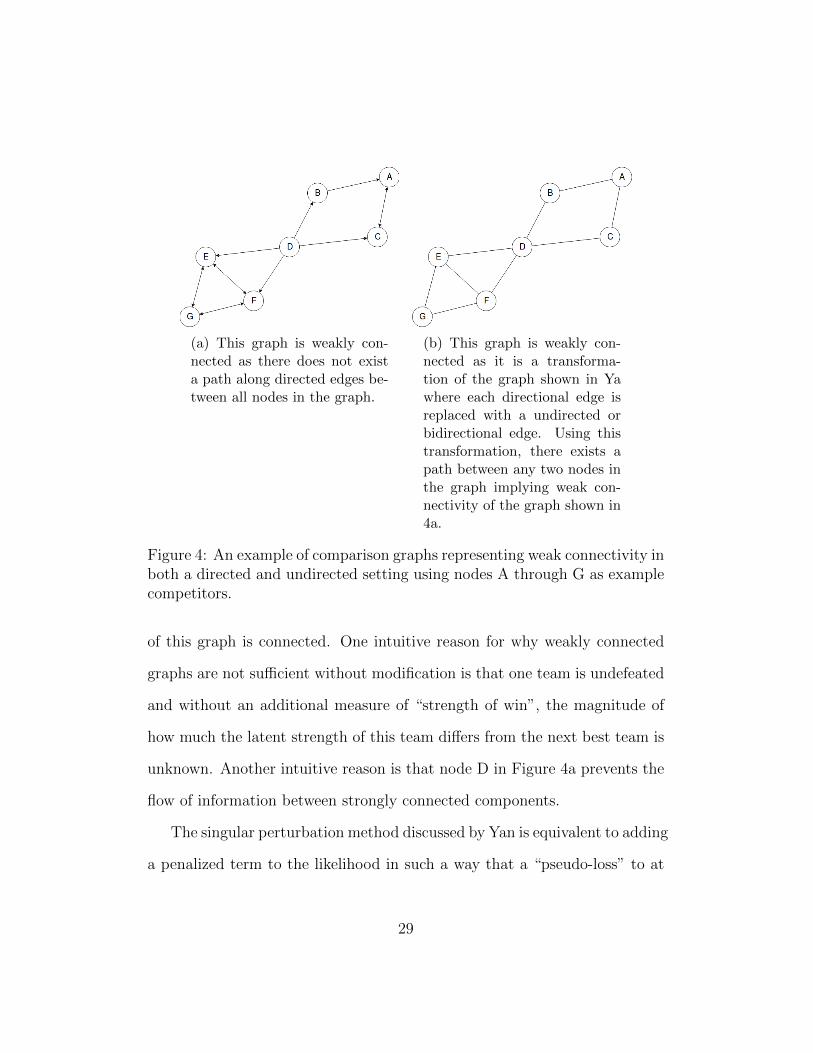
(a) This graph is weakly con-nected as there does not exista path along directed edges be-tween all nodes in the graph.

(b) This graph is weakly con-nected as it is a transforma-tion of the graph shown in Yawhere each directional edge isreplaced with a undirected orbidirectional edge. Using thistransformation, there exists apath between any two nodes inthe graph implying weak con-nectivity of the graph shown in4a.

Figure 4: An example of comparison graphs representing weak connectivity inboth a directed and undirected setting using nodes A through G as examplecompetitors.

of this graph is connected. One intuitive reason for why weakly connected

graphs are not sufficient without modification is that one team is undefeated

and without an additional measure of “strength of win”, the magnitude of

how much the latent strength of this team differs from the next best team is

unknown. Another intuitive reason is that node D in Figure 4a prevents the

flow of information between strongly connected components.

The singular perturbation method discussed by Yan is equivalent to adding

a penalized term to the likelihood in such a way that a “pseudo-loss” to at

29

least one other team is added to the comparison graph in order for the graph

to become strongly connected. This penalizer term can be re-interpreted as

a specific prior distribution. Depending on the framework being employed,

the prior distribution will differ. The next section reveals why this method

was not required for large datasets, but can be adapted depending on the

needs of the dataset.

3.4 Simulation of Graph Connectivity

It is useful to understand how likely a graph is to be connected given some

properties (number of nodes, number of edges). Assessing the probability of

a graph being connected is a difficult combinatorial problem to solve ana-

lytically. However, it is possible to simulate the connectedness of a graph.

In the case of the data we are analyzing, we assume that two characters

are randomly chosen to participate in a match. This is a strong assump-

tion about the underlying structure of how characters are chosen for a given

match. Specifically, it is unclear if SaltyBet uses any heuristic beyond ran-

domness to choose characters for each match. This could be analyzed by

attempting to determine if there are clusters of nodes within the comparison

graph of SaltyBet matches which have a higher connectivity to other nodes.

Unfortunately, the problem of detecting “densely” connected clusters within

a graph is computationally challenging as well and is beyond the scope of this

project [19]. Instead, we will assume that of the 9,662 characters present,

two characters are randomly chosen and then compared within a match. For

30

our simulation, we will allow the order in which the characters are chosen to

correspond to the direction of the edge between each character with the first

character being chosen denoted as the winner of the match. This equates to

an expected 50% win rate for each character. While this does not account for

the underlying strength of a character, it provides a general enough frame-

work for an intuition to be formed around how many matches are needed to

be strongly connected.

The simulation begins by generating 9,662 nodes and then randomly gen-

erating directed edges between them. The number of edges generated varies

from 100,000 to 1,500,000 in steps of 100,000 with 25 simulated comparison

graphs being generated at each step. We then apply Tarjan’s Algorithm to

determine the number of strongly connected components within each graph.

In parallel to this experiment, we also measure the number of weakly con-

nected components within each graph simulated. The results of the sim-

ulation revealed that a lower number of directed edges are required than

expected in order for the graph to be strongly connected. Only the simu-

lated comparison graphs consisting of 100,000 edges had results which were

not entirely strongly connected. In the case of the 100,000 edges, out of the

25 simulations performed there were an average of 1.56 strongly connected

components per graph. Specifically, 12 of the 25 simulations had more than

one strongly connected component or the graphs simulated were not entirely

strongly connected. In the case of weakly connected components, since the

condition is weaker than being entirely strongly connected, all simulations

31

returned that the graph was weakly connected at 100,000 edges and greater.

While this is an approximation using assumptions previously discussed, this

does provide evidence connectivity will not be an issue for the dataset in

question or when the number of edges is at least one order of magnitude

larger than the number of nodes. Code used to perform this simulation is

available in the code repository made available via the code appendix.

4 Data Analysis

4.1 Data Collection

For this project, historic matches were scraped from the SaltyBet website

through the premium functionality which allows previous match data to be

accessed. Since the site requires a login, a dynamic web scraping framework

was required. The code appendix contains the scripts used to obtain the

data. There were a total of 946,172 matches between 9,662 characters in the

final dataset.

Within SaltyBet, characters are divided into five distinct tiers: X, S, A,

B, and P. These tiers are assigned based on the performance of each character

previously. Characters are promoted or demoted based on their performance

directly after a match. There are three distinct types of matches: matchmak-

ing, tournament, and exhibition. The matchmaking mode algorithmically

chooses players to match up against each other where the odds are approxi-

mately equal of each character winning. Tournament mode is a random set of

32

16 characters from a specific tier who fight each other in a single-elimination

tournament. Finally, exhibition mode is a set of viewer-requested matches

which also allows teams of characters to compete. Exhibition mode games

are typically chosen by viewers to force edge-case behavior of the characters.

Many times, viewer requested matches result in a server crash due to intense

computational loads. Each of these factors are important as we begin to

make decisions on how best to clean the data.

4.2 Data Cleaning

With the major components of modeling, estimation, and diagnostic of this

project having been discussed in detail, we begin the analysis of the Salty-

Bet data collected. First, we note some data cleaning steps. As discussed

previously, SaltyBet consists of three phases: matchmaking, exhibition, and

tournament. Within the exhibition mode teams of two characters are allowed

to be requested by viewers. Since the data does not specify the makeup of

each team, we remove matches which contain any team of characters. This

accounts for 84,892 matches of the entire dataset. In addition, while ties

are both permitted by SaltyBet and literature exists to incorporate this into

the Bradley-Terry models, we remove them from this dataset for a number

of reasons. First, ties are unlikely within SaltyBet consisting of only 5050

matches. Second, if a tie does occur, it is typically due to either server fail-

ure or some unique attribute of the match up of characters. Matches which

consist of the same character fighting itself are removed as it is assumed no

33

character can play itself in Bradley-Terry models. This consists of only 76

matches of the dataset.

When cleaning the character dataset, there are some character images

which were not available. In total, there were 153 characters with missing

hitbox information. These characters were removed from the dataset entirely.

This resulted in a loss of an additional 28,846 matches from the dataset.

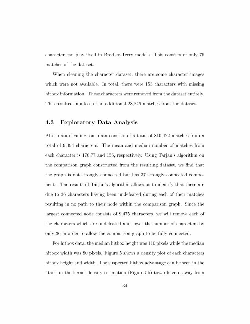
4.3 Exploratory Data Analysis

After data cleaning, our data consists of a total of 810,422 matches from a

total of 9,494 characters. The mean and median number of matches from

each character is 170.77 and 156, respectively. Using Tarjan’s algorithm on

the comparison graph constructed from the resulting dataset, we find that

the graph is not strongly connected but has 37 strongly connected compo-

nents. The results of Tarjan’s algorithm allows us to identify that these are

due to 36 characters having been undefeated during each of their matches

resulting in no path to their node within the comparison graph. Since the

largest connected node consists of 9,475 characters, we will remove each of

the characters which are undefeated and lower the number of characters by

only 36 in order to allow the comparison graph to be fully connected.

For hitbox data, the median hitbox height was 110 pixels while the median

hitbox width was 80 pixels. Figure 5 shows a density plot of each characters

hitbox height and width. The suspected hitbox advantage can be seen in the

“tail” in the kernel density estimation (Figure 5b) towards zero away from

34

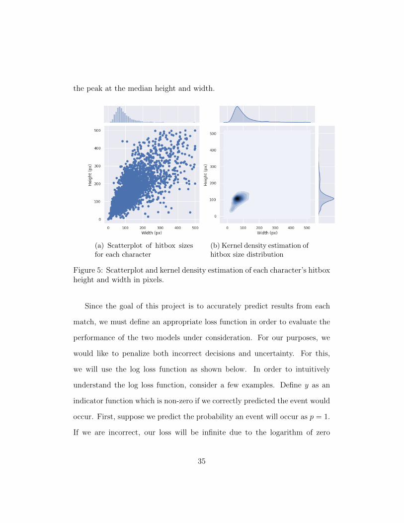
the peak at the median height and width.

(a) Scatterplot of hitbox sizesfor each character

(b) Kernel density estimation ofhitbox size distribution

Figure 5: Scatterplot and kernel density estimation of each character’s hitboxheight and width in pixels.

Since the goal of this project is to accurately predict results from each

match, we must define an appropriate loss function in order to evaluate the

performance of the two models under consideration. For our purposes, we

would like to penalize both incorrect decisions and uncertainty. For this,

we will use the log loss function as shown below. In order to intuitively

understand the log loss function, consider a few examples. Define y as an

indicator function which is non-zero if we correctly predicted the event would

occur. First, suppose we predict the probability an event will occur as p = 1.

If we are incorrect, our loss will be infinite due to the logarithm of zero

35

being mathematically undefined at infinity. Likewise, if the opposite situation

occurs we also obtain an infinite loss. Therefore, we are forced to express

some uncertainty about the event in the form of p being bounded between

zero and one. One potentially safe strategy is to simply choose p = 0.5 for

each match. This could be a sound strategy except that the loss function is

maximized at the value of p = 0.5 when not equal to zero or one. Therefore,

this loss function will penalize for incorrect decisions but also the amount of

uncertainty around correct decisions.

LogLoss(p) = ylog(p)− (1− y)log(1− p)

In order to test the predictive models constructed, the dataset is divided

into training and test sets. The test set consists of 10,000 randomly sampled

matches from the cleaned dataset while the training set consists of the re-

mainder of the data. Each model is fit using the training set and the log loss

function is evaluated for each prediction of the 10,000 overall. Two metrics

are examined as part of the prediction: the median log loss of each match

prediction as well as the cumulative log loss over all matches.

4.4 Prediction results of Basic Bradley-Terry model

Using the basic Bradley-Terry formulation we fit the model using code devel-

oped by Coran and Doucet for their publication. In order to fit the model,

we construct a comparison graph from the dataset provided. We provide

36

this to the model as a dataset and perform 10,000 iterations of sampling

with a 1,000 iteration burn-in period. The model shows no concerns with

convergence. We evaluate the result of the model using the estimated la-

tent strengths of each character and the associated probability statement to

obtain an estimated value of p for a given match. Over the set of 10,000

test matches, we have a mean loss of -0.5697. We will fit and predict the

same dataset using the “home-field advantage” model and then compare the

results between the two models. For both models, a prior distribution with

parameters a = 5 were used for the analysis.

4.5 Prediction Results of Advantage Bradley-Terry model

Again, we turn to the code developed by Coran and Doucet for their pub-

lication to fit this model. The dataset required by this model differs in

that a comparison graph needs to be constructed for the two different types

of matches which are permitted: advantaged and disadvantaged matches.

Therefore, we construct a comparison graph of each character when they

had advantaged wins and another for when they had disadvantaged wins.

If these two matrices are summed, we obtain the win matrix used in the

basic formulation of this model. Again, we see no issues with convergence

by dividing the parameters out into sections to obtain a better view of con-

vergence in the appendix. Performing the same test as before, we see that

we have a mean loss of -1.5602 over the 10,000 test matches. A histogram

of the posterior distribution of λ, the advantage term, is shown in Figure

37

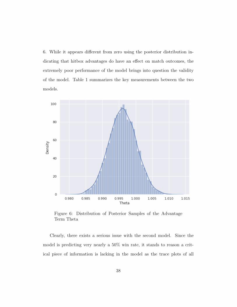
6. While it appears different from zero using the posterior distribution in-

dicating that hitbox advantages do have an effect on match outcomes, the

extremely poor performance of the model brings into question the validity

of the model. Table 1 summarizes the key measurements between the two

models.

Figure 6: Distribution of Posterior Samples of the AdvantageTerm Theta

Clearly, there exists a serious issue with the second model. Since the

model is predicting very nearly a 50% win rate, it stands to reason a crit-

ical piece of information is lacking in the model as the trace plots of all

38

Table 1: Summary of predictive model results

Model % Correct Mean Log Loss Cumulative Log LossBasic 71.57% -0.5697 -374180095Advantage 49.71% -1.5602 -1024765811

parameters appear to have no convergence issues. One possibility is that

the comparison graph of the advantaged model has additional assumptions.

It has not been stated within literature that it is a requirement that both

comparison graphs constructed from advantaged and disadvantaged matches

be connected. However, in the case of this analysis, comparison graph con-

nectivity appears to be a potential issue. When applying Tarjan’s algorithm

to each of these comparison graphs separately we see that the majority of

the components are disconnected for hitbox advantaged and disadvantaged

wins with 9,453 and 9,133 strongly connected components, respectively. This

could potentially explain the the poor predictive performance of the advan-

tage model compared to the basic model which had a strongly connected

graph for the vast majority of its nodes. No literature found discusses if the

requirement of connectivity changes for “home-field advantage” models. It

may be the case that since advantages in this dataset are strictly one-sided (if

character A has a smaller hitbox than character B, character A will have the

advantage in all matches against B), we have a much larger required number

of connections in the advantage case in order for the comparison graph to

be strongly connected. Regardless, the extremely poor performance of this

model using this dataset requires further investigation as future work.

39

5 Conclusions & Future Work

In this project, we reviewed two specific formulations of paired-comparison

models. First, we developed the background around the basic Bradley-Terry

model and then discussed in more detail the “home-field advantage” model

developed by Agresti. We reviewed estimation techniques for both models in-

cluding the original algorithm developed by Zermelo and continuing on to the

general class of Minorization-Maximization algorithms discussed in detail by

Hunter. We ended our estimation discussion with a detailed look at methods

for efficient Bayesian estimation of Bradley-Terry models by summarizing the

work of Coran and Doucet. In this paper, we discussed the Gibbs samplers

developed for both the basic and “home-field advantage” models which were

made possible by a specific latent variable definition.

Before discussing the analysis of the dataset, we reviewed the necessary

assumptions required of the comparison graph constructed from the dataset.

Specifically, we defined two different types of connectivity associated with

graphs known as strong-connectivity and weak-connectivity and discussed

their interpretations and implications on paired-comparison datasets. Fi-

nally, we discussed how to determine if assumptions of connectivity are met

using Tarjan’s algorithm and reviewed the work of Yao in the case of only

having weak connectivity. Examples of different types of connectivity were

shown and discussed visually.

Finally, we used the theory developed in the project to perform a large

40

scale prediction project using SaltyBet data. Both the basic and “home-field

advantage” model were employed where the advantage in this context was

determined by each characters relative hitbox size. The basic model pro-

vided moderate predictive capability with an overall correct prediction rate

of approximately 72%. This is a high level of accuracy given that matches

are suspected to be designed to provide even odds between each character.

The “home-field advantage” model added no predictive power over randomly

guessing. This is suspected to be due to a different type of comparison

graph connectivity requirement for advantage models compared to the basic

Bradley-Terry model. In this case, since the components were almost en-

tirely disconnected, the comparisons between the majority of the nodes were

essentially random guesses by the model.

The most obvious extension of this work is to investigate further the

requirement for connectivity within “home-field advantage” Bradley-Terry

models. This dataset may be a special case as the advantages are one-

sided through all matches between any two characters (a character’s hitbox

is static). In many other scenarios, “home-field advantage” shifts between

two teams multiple times so that there are many comparisons to simultane-

ously estimate the latent strength and effect of any “home-field advantage”.

It is possible that the one-sided nature of hitbox advantages is not amenable

to this modeling approach. If it is not, future work could investigate other

modeling approaches to incorporate this effect. Other extensions include

extending either the basic Bradley-Terry model used in this project or an

41

altered advantage model to incorporate a Markov decision process element.

This can be extended further to automating this system to automatically

perform bets on SaltyBet.com and track betting strategies.

42

6 References

[1] 10 helpful ways to get you out of the Salt Mines in Salty Bet. 2017.

url: https://www.gamezone.com/originals/10-helpful-ways-

to-get-you-out-of-the-salt-mines-in-salty-bet/.

[2] Alan Agresti and Maria Kateri. Categorical data analysis. Springer,

2011.

[3] Automating SaltyBet - My Live and Ongoing Adventure - DONE!! url:

https://www.giantbomb.com/profile/tycobb/blog/automating-

saltybet-my-live-and-ongoing-adventure-/102462/.

[4] Ralph Allan Bradley and Milton E. Terry. “Rank Analysis of Incom-

plete Block Designs: I. The Method of Paired Comparisons”. In: Biometrika

39.3/4 (1952), p. 324. doi: 10.2307/2334029.

[5] CAPCOM — History. url: http://www.capcom.co.jp/ir/english/

company/history.html.

[6] Francois Caron and Arnaud Doucet. “Efficient Bayesian inference for

generalized Bradley–Terry models”. In: Journal of Computational and

Graphical Statistics 21.1 (2012), pp. 174–196.

[7] George Casella and Roger L Berger. Statistical inference. Vol. 2. Duxbury

Pacific Grove, CA, 2002.

43

[8] Paul Campos Chait and Jonathan. Sabermetrics for Football. 2004.

url: https://www.nytimes.com/2004/12/12/magazine/sabermetrics-

for-football.html.

[9] Gary Chartrand. Introductory graph theory. Dover Publications, Inc.,

1985.

[10] Roger R Davidson. “On extending the Bradley-Terry model to ac-

commodate ties in paired comparison experiments”. In: Journal of the

American Statistical Association 65.329 (1970), pp. 317–328.

[11] Shouvik Dutta, Sheldon H Jacobson, and Jason J Sauppe. “Identi-

fying NCAA tournament upsets using Balance Optimization Subset

Selection”. In: Journal of Quantitative Analysis in Sports 13.2 (2017),

pp. 79–93.

[12] L. R. Ford. “Solution of a Ranking Problem from Binary Comparisons”.

In: The American Mathematical Monthly 64.8 (1957), p. 28. doi: 10.

2307/2308513.

[13] Andrew Gelman, Donald B Rubin, et al. “Inference from iterative sim-

ulation using multiple sequences”. In: Statistical science 7.4 (1992),

pp. 457–472.

[14] Have You Played... Salty Bet? url: https://www.rockpapershotgun.

com/2017/12/15/have-you-played-salty-bet/.

[15] Monson H. Hayes. Statistical Digital Signal Processing and Modeling.

Wiley, 2014.

44

[16] Willem J Heiser. “Convergent computation by iterative majorization:

theory and applications in multidimensional data analysis”. In: Recent

advances in descriptive multivariate analysis (1995), pp. 157–189.

[17] Kyle Hilliard. An Interview With The Mind Behind Twitch Plays Pokemon.

url: https://www.gameinformer.com/b/features/archive/2014/

03/14/an-interview-with-the-mind-behind-twitch-plays-pok-

233-mon.aspx.

[18] David R Hunter et al. “MM algorithms for generalized Bradley-Terry

models”. In: The annals of statistics 32.1 (2004), pp. 384–406.

[19] Samir Khuller and Barna Saha. “On finding dense subgraphs”. In: In-

ternational Colloquium on Automata, Languages, and Programming.

Springer. 2009, pp. 597–608.

[20] Mykel J. Kochenderfer. Decision making under uncertainty: theory and

application. The MIT Press, 2015.

[21] Kenneth Lange, David R Hunter, and Ilsoon Yang. “Optimization

transfer using surrogate objective functions”. In: Journal of compu-

tational and graphical statistics 9.1 (2000), pp. 1–20.

[22] Patrick Miller. Sodium Intake: An Interview with the Creator of Salty

Bet. 2013. url: http : / / shoryuken . com / 2013 / 08 / 12 / sodium -

intake-an-interview-with-the-creator-of-salty-bet/.

[23] M.U.G.E.N. 2019. url: https://en.wikipedia.org/wiki/M.U.G.E.

N.

45

[24] D. S. G. Pollock. Recursive Estimationand the Kalman Filter. url:

https://www.le.ac.uk/users/dsgp1/COURSES/MESOMET/ECMETXT/

recurse.pdf.

[25] Sports Roundtable. The ’Moneyball’ Effect: Are Sabermetrics Good for

Sports? 2013. url: https://www.theatlantic.com/entertainment/

archive/2011/09/the- moneyball- effect- are- sabermetrics-

good-for-sports/244453/.

[26] Darren Rovell. Class action lawsuit filed against DraftKings and Fan-

Duel. 2015. url: http : / / www . espn . com / chalk / story / _ / id /

13840184/class-action-lawsuit-accuses-draftkings-fanduel-

negligence-fraud-false-advertising.

[27] Francisco JR Ruiz and Fernando Perez-Cruz. “A generative model for

predicting outcomes in college basketball”. In: Journal of Quantitative

Analysis in Sports 11.1 (2015), pp. 39–52.

[28] SaltyBet. Salty Bet (@SaltyBet). 2013. url: https://twitter.com/

saltybet.

[29] SpriteClub. url: https://mugen.spriteclub.tv/.

[30] Story of a Betting Bot. url: https://explosionduck.com/wp/story-

of-a-betting-bot/.

[31] Synkarius. synkarius/saltbot. 2019. url: https://github.com/synkarius/

saltbot.

46

[32] Robert Tarjan. “Depth-first search and linear graph algorithms”. In:

12th Annual Symposium on Switching and Automata Theory (swat

1971) (1971). doi: 10.1109/swat.1971.10.

[33] L. L. Thurstone. “A law of comparative judgment.” In: Psychological

Review 34.4 (1927), 273–286. doi: 10.1037/h0070288.

[34] Twitch analytics and statistics. url: http://sullygnome.com/.

[35] Philippa Warr. Salty Bet: a pop culture royal rumble we can’t stop

watching. 2013. url: https://www.pcgamer.com/salty-bet-1/.

[36] What is Salty Bet? The Salty Bet Beginners Guide. 2013. url: http:

//calmdowntom.com/2013/08/what-is-salty-bet/.

[37] John. T Whelan. Using Bayesian statistics to rank sports teams (or,

my replacement for the BCS). Talk. 2010. url: https://ccrg.rit.

edu/~whelan/talks/whelan20101008.pdf.

[38] Leo Wichtowski. Place Bets On Computers Playing Fighting Games

Against Each Other. 2013. url: https://kotaku.com/place-bets-

on-computers-playing-fighting-games-against-1148194469.

[39] Ting Yan. “Ranking in the generalized Bradley–Terry models when the

strong connection condition fails”. In: Communications in Statistics-

Theory and Methods 45.2 (2016), pp. 340–353.

[40] Grace Yao and Ulf Bockenholt. “Bayesian estimation of Thurstonian

ranking models based on the Gibbs sampler”. In: British Journal of

47

Mathematical and Statistical Psychology 52.1 (1999), 79–92. doi: 10.

1348/000711099158973.

48

7 Code Appendix

The code appendix for this project can be found online at github.com/EriqLaplus/msu-

writing-project.

49