Predicting Molecular Properties with Covariant Compositional NetworksTruong Son Hy,1 Shubhendu Trivedi,2 Horace Pan,1 Brandon M. Anderson,1 and Risi Kondor1, 3, a)1)Department of Computer Science, The University of Chicago2)Toyota Technological Institute at Chicago3)Department of Statistics, The University of Chicago

( Dated: 2 June 2018)

Density functional theory (DFT) is the most successful and widely used approach for computing the electronicstructure of matter. However, for tasks involving large sets of candidate molecules, running DFT separatelyfor every possible compound of interest is forbiddingly expensive. In this paper, we propose a neural networkbased machine learning algorithm which, assuming a sufficiently large training sample of actual DFT results,can instead learn to predict certain properties of molecules purely from their molecular graphs. Our algorithmis based on the recently proposed covariant compositional networks (CCN) framework, and involves tensorreduction operations that are covariant with respect to permutations of the atoms. This new approach avoidssome of the representational limitations of other neural networks that are popular in learning from moleculargraphs, and yields promising results in numerical experiments on the Harvard Clean Energy Project and QM9molecular datasets.

I. INTRODUCTION

Density functional theory1 (DFT) is the workhorse ofmodern quantum chemistry, due to its ability to calcu-late many properties of molecular systems with high ac-curacy. However, this accuracy comes at a significantcomputational cost, generally making DFT too costly forapplications such as chemical search and drug screening,which may involve hundreds of thousands of compounds.Methods that help overcome this limitation could lead torapid developments in biology, medicine, and materialsengineering.

Recent advances in machine learning, specifically,deep learning2, combined with the appearance of largedatasets of molecular properties obtained both experi-mentally and theoretically3–5 present an opportunity tolearn to predict the properties of compunds from theirchemical structure rather than computing them explic-itly with DFT. A machine learning model could allow forrapid and accurate exploration of huge molecular spacesto find suitable candidates for a desired molecule.

Central to any machine learning technique is the choiceof a suitable set of descriptors, or features used toparametrize and describe the input data. A poor choiceof features will limit the expressiveness of the learning ar-chitecture and make accurate predictions impossible. Onthe other hand, providing too many features may maketraining difficult, especially when training data is limited.Hence, there has a been a significant amount of workon designing good features for molecular systems. Pre-dictions of energetics based on molecular geometry havebeen explored extensively, using a variety of parametriza-tions6,7. This includes bond types and/or angles8, radialdistance distributions9, the Coulomb matrix and relatedstructures10–12, the Smooth Overlap of Atomic Positions(SOAP)13,14, permutation-invariant distances15, symme-

a)Electronic mail: risi@cs.uchicago.edu

try functions for atomic positions16,17, Moment TensorPotentials18, and Scattering Networks19.

Recently, the problem of learning from the structureof chemical bonds alone, i.e., the molecular graph, hasattracted a lot of interest, especially in light of the ap-pearance of a series of neural network architectures de-signed specifically for learning from graphs20–26. Muchof the success of these architectures stems from theirability to pick up on structure in the graph at multi-ple different scales, while satisfying the crucial require-ment that the output be invariant to permutations ofthe vertices (which, in molecular learning, correspond toatoms). However, as will explain, the specific way thatmost of these architectures ensure permutation invari-ance still limits their representaional power.

In this paper, we propose a new type of neural net-work for learning from molecular graphs, based on thethe idea of covariant compositional networks (CCNs),recently introduced in Ref 27. Importantly, CCNs arebased on explicitly decomposing compound objects (inour case, molecular graphs) into a hierarchy of subparts(subgraphs), offering a versatile framework that is ideallysuited to capturing the multiscale nature of molecularstructures from functional groups through local structureto overall shape. In a certain sense, the resulting modelsare the neural networks analog of coarse graining. In ad-dition, CCNs offer a more nuanced take on permutationinvariance than other graph learning algorithms: whilethe overall output of a CCN is still invariant to the per-mutation of identical atoms, internally, the activations ofthe network are covariant rather than invariant, allowingus to better preserve information about the relationshipsbetween atoms. We demonstrate the success of this ar-chitecture through experiments on benchmark datasets,including QM93 and the Harvard Clean Energy Project4.

2

f1

n1

f2

n2

f3

n3

f4

n4

f5

n5

f6

n6

f7

n7

f8

n8

f9

n9

f10

n10

fr nr

FIG. 1. Left: Molecular graphs for C18H9N3OSSe and C22H15NSeSi from the Harvard Clean Enery Project (HCEP)4 datasetwith corresponding adjacency matrices. Center and right: The comp-net of a graph G is constructed by decomposing Ginto a hierarchy of subgraphs {Pi} and forming a neural network N in which each “neuron” ni corresponds to one of the Pi

subgraphs, and receives inputs from other neurons that correspond to smaller subgraphs contained in Pi. The center paneshows how this can equivalently be thought of as an algorithm in which each vertex of G receives and aggregates messages fromits neighbors. To keep the figure simple, we only marked aggregation at a single vertex in each round (layer).

II. LEARNING FROM MOLECULAR GRAPHS

This paper addresses the problem of predicting chem-ical properties directly from each compound’s molecu-lar graph, which we will denote G (Figure 1, left). Assuch, it is related to the sizable literature on learningfrom graphs. In the kernel machines domain this in-cludes algorithms based on random walks28–30, countingsubgraphs31, spectral ideas32, label propagation schemeswith hashing33,34, and even algebraic ideas35.

Recently, a sequence of neural network based ap-proaches have also appeared, starting with Ref. 36. Someof the proposed graph learning architectures21,22,37 di-rectly seek inspiration from the type of classical convo-lutional neural networks (CNNs) that are used for imagerecognition38,39. These methods involve moving a filteracross vertices to create feature representations of eachvertex based on its local neighborhoods. Other notableworks on graph neural networks include Refs. 24, 40–42. Very recently, Ref. 25 showed that many of theseapproaches can be seen as message passing schemes,and coined the term message passing neural networks(MPNNs) to refer to them collectively.

Regardless of the specifics, the two major issues thatgraph learning methods need to grapple with are invari-ance to permutations and capturing structure at multipledifferent scales. Let A denote the adjacency matrix of G,and suppose that we change the numbering of the ver-tices by applying a permutation σ. The adjacency matrixwill then change to A′, with

A′i,j = Aσ−1(i),σ−1(j).

However, topologically, A and A′ still represent the samegraph. Permutation invariance means that the represen-

tation φ(G) learned or implied by our graph learning al-gorithm must be invariant to these transformations. Nat-urally, in the case of molecules, invariance is restricted topermutations that map each atom to another atom of thesame type.

The multiscale property is equally crucial for learningmolecular properties. For example, in the case of a pro-tein, an ideal graph learning algorithm would representG in a manner that simultaneously captures structure atthe level of individual atoms, functional groups, interac-tions between functional groups, subunits of the protein,and the protein’s overall shape.

A. Compositional networks

The idea of representing complex objects in termsof a hierarchy of parts has a long history in machinelearning43–48. We have recently introduced a generalframework for encoding such part-based models in a spe-cial type of neural network, called covariant composi-tional networks (CCNs)27. In this paper we show howthe CCN formalism can be specialized to learning fromgraphs, specifically, the graphs of molecules. Our startingpoint is the following definition.

Definition 1 Let G be the graph of a molecule made upof n atoms {e1, . . . , en}. The compositional neuralnetwork (comp-net) corresponding to G is a directedacyclic graph (DAG) N in which each node (neuron) niis associated with a subgraph Pi of G and carries an ac-tivation fi. Moreover,1. If ni is a leaf node, then Pi is just a single vertex ofG, i.e., an atom eξ(i), and the activation fi, is someinitial label li. In the simplest case, fi is a “one-hot”

3

Algorithm 1 High level schematic of message passingtype algorithms25 in the notations of the present paper.Here li are the starting labels, and nei1, . . . ,neik denotethe neighbors of vertex i.for each vertex i

f0i ← li

for `= 1 to Lfor each vertex if `i ← Ψ(f `−1

nei1, . . . , f `−1

neik)

φ(G) ≡ fr ← Ψr(fL1 , . . . , f

Ln )

vector that identifies what type of atom resides at thegiven vertex.

2. N has a unique root node nr for which Pr = G, andthe corresponding fr represents the entire molecule.

3. For any two nodes ni and nj, if ni is a descendant ofnj, then Pi is a subgraph of Pj, and

fi = Φi(fc1 , fc2 , . . . , fck),

where fc1 , . . . , fck denote the activations of the chil-dren of ni. Here, Φi is called the aggregation functionof node i.

Note that we now have two separate graphs: the originalgraph G, and the networkN that represents the “is a sub-graph of” relationships between different subgraphs of G.One of the fundamantal ideas of this paper is that N canbe interpreted as a neural network, in which each node niis a “neuron” that receives inputs (fc1 , fc2 , . . . , fck) andoutputs the activation fi = Φi(fc1 , fc2 , . . . , fck) (Figure1, right). For now we treat the activations as vectors,but will soon generalize them to be tensors.

There is some freedom in how the system {Pi} of sub-graphs is defined, but the default choice is {P`i }, whereP`i is the subgraph of vertices within a radius of ` of ver-tex i. In this case, P0

i = {i}, P` consits of the immediateneighbors of i, plus i itself, and so on. The aggregationfunction is discussed in detail in Section IV.

Conceptually, comp-nets are closely related to convo-lutional neural networks (CNNs), which are the mainstayof neural networks in computer vision. In particular,1. Each neuron in a CNN only aggregates information

from a small set of neurons from the previous layer,similarly to how each node of a comp-net only aggre-gates information from its children.

2. The so-called effective receptive fields of the neuronsin a CNN, i.e., the image patches for which each neu-ron is responsible for, form a hierarchy of nested setssimilar to the hierarchy of {Pi} subgraphs.

In this sense, CNNs are a specific kind of compositionalnetwork, where the atoms are pixels. Because of thisanalogy, in the following we will sometimes refer to Pi asthe receptive field of neuron i, dropping the “effective”qualifier for brevity.

As mentioned above, an alternative popular frameworkfor learning from graphs is message passing neural net-works (MPNNs)25. An MPNN operates in rounds: in

each round ` = 1, . . . , L, every vertex collects the la-bels of its immediate neighbors, applies a nonlinear func-tion Ψ, and updates its own label accordingly. Fromthe neural networks point of view, the rounds corre-spond to layers and the labels correspond to the f `iactivations (Algorithm 1). More broadly, the classicWeisfeiler–Lehman test of isomorphism follows the samelogic49–51, and so does the related Weisfeiler–Lehmankernel, arguably the most successful kernel-based ap-proach to graph learning33.

In the above mentioned base case when {P`i } is thecollection of all subgraphs of G of radii ` = 0, 1, 2, . . .,a comp-net can also be thought of as a message passingalgorithm: the messages received by vertex i in round` are the activations {f `−1uj | uj ∈B(i, 1)}, where B(i, 1)

is the ball of radius one centered at i (note that thiscontains not just the neighbors of i, but also i itself).Conversely, MPNNs can be seen as comp-nets, where P`iis the subgraph defined by the receptive field of vertex iin round `. A common feature of MPNNs, however, isthat the Ψ aggregation functions that they employ areinvariant to permuting their arguments. Most often, Ψjust sums all incoming messages and then applies a non-linearity. This certainly guarantees that the final outputof the network, φ(G) = fr, will be permutation invariant.However, in the next section we argue that it comes atthe price of a significant loss of representational power.

III. COVARIANT COMPOSITIONAL NETWORKS

One of the messages of the present paper is that in-variant aggregation functions, of the type popularizedby message passing neural networks, are not the mostgeneral way to build compositional models for compoundobjects, such as graphs. To understand why this is thecase, once again, an analogy with image recognition ishelpful. Classical CNNs face two types of basic imagetransformations: translations and rotations. With re-spect to translations (barring pooling, edge effects andother complications), CNNs behave in a quasi-invariantway, in the sense that if the input image is translated byan integer amount (tx, ty), the activations in each layer` = 1, 2, . . . L translate the same way: the activation ofneuron n`i,j is simply transferred to neuron n`i+t1,j+t2 , i.e.,f ′`i+t1,j+t2= f `i,j . This is the simplest manifestation of awell studied property of CNNs called equivariance52,53.

With respect to rotations, however, the situation ismore complicated: if we rotate the input image by, e.g.,90 degrees, not only will the part of the image that fellin the receptive field of neuron n`i,j move to the receptive

field of a different neuron n`−j,i, but the orientation ofthe receptive field will also change. For example, featureswhich were previously picked up by horizontal filters willnow be picked up by vertical filters. Therefore, in general,f ′`−j,i 6=f `i,j (Figure 2).

It can be shown that one cannot construct a CNN forimages that behaves in a quasi-invariant way with respect

4

FIG. 2. In a convolutional neural network if the input imageis translated by some amount (t1, t2), what used to fall inthe receptive field of neuron n`i,j is moved to the receptivefield of n`i+t1,j+t2 . Therefore, the activations transform in thevery simple way f ′`i+t1,j+t2 = f `

i,j . In contrast, rotations notonly move the receptive fields around, but also permute theneurons in the receptive field internally, so the activationstransform in a more complicated manner. The right handfigure shows that if the CNN has a horizontal filter (blue)and a vertical one (red), then after a rotation by 90 degrees,their activations are exchanged. In steerable CNNs, if (i, j) ismoved to (i′, j′) by the transformation, then f ′`i′,j′ =R(f `

i,j),where R is some fixed linear function of the rotation angle.

to both translations and rotations, unless every filter isdirectionless. It is, however, possible to construct a CNNin which the activations transform in a predictable andreversible way, f ′`−j,i = R(f `i,j), for some fixed functionR. This phenomenon is called steerability, and has a sig-nificant literature in both classical signal processing54–58

and the neural networks field59.

The situation in compositional networks is similar.The comp-net and message passing architectures thatwe have examined so far, by virtue of the aggregationfunction being symmetric in its arguments, are all quasi-invariant (with respect to permutations) in the sensethat if N and N ′ are two comp-nets for the same graphdiffering only in a reordering σ of the vertices of the un-derlying graph G, and ni is a neuron in N while n′j isthe corresponding neuron in N ′, then fi = f ′j for anypermutation σ ∈ Sn.

Quasi-invariance amounts to asserting that the acti-vation fi at any given node must only depend on Pi ={ej1 , . . . , ejk} as a set, and not on the internal ordering ofthe atoms ej1 , . . . , ejk making up the receptive field. Atfirst sight this seems desirable, since it is exactly what weexpect from the overall representation φ(G). On closerexamination, however, we realize that this property ispotentially problematic, since it means that ni loses all

1

32

4 5 65′

1

32

4 5 6

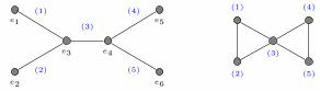
FIG. 3. These two graphs are not isomorphic, but after asingle round of message passing (red arrows), the labels (ac-tivations) at vertices 2 and 3 will be identical in both graphs.Therefore, in the second round of message passing vertex 1will get the same messages in both graphs (blue arrows), andwill have no way of distinguishing whether 5 and 5′ are thesame vertex or not.

information about which vertex in its receptive field hascontributed what to the aggregate information fi. In theCNN analogy, we can say that we have lost informationabout the orientation of the receptive field. In particu-lar, if higher up in the network fi is combined with someother feature vector fj from a node with an overlappingreceptive field, the aggregation process has no way oftaking into account which parts of the information in fiand fj come from shared vertices and which parts do not(Figure 3).

The solution is to regard the Pi receptive fields as or-dered sets, and explicitly establish how fi co-varies withthe internal ordering of the receptive fields. To empha-size that henceforth the Pi sets are ordered, we will useparentheses rather than braces to denote them.

Definition 2 Assume that N is the comp-net of a graphG, and N ′ is the comp-net of the same graph but afterits vertices have been permuted by some permutation σ.Given any ni ∈N with receptive field Pi = (ep1 , . . . , epm),let n′j be the corresponding node in N ′ with receptive fieldP ′j = (eq1 , . . . , eqm). Assume that π ∈ Sm is the permuta-tion that aligns the orderings of the two receptive fields,i.e., for which eqπ(a)

= epa . We say that the comp-netsare covariant to permutations if for any π, there is acorresponding function Rπ such that f ′j = Rπ(fi).

To make the form of covariance prescribed by this def-inition more specific, we make the assumption that the{f 7→ Rπ(f)}π∈Sm maps are linear. This allows us totreat them as matrices, {Rπ}π∈Sn . Furthermore, linear-ity also implies that {Rπ}π∈Sm form a representation ofSm in the group theoretic sense of the word60(this notion

5

e1

e2

e3 e4

e5

e6

`= 0

e1

e2

e3 e4

e5

e6

`= 1

e1

e2

e3 e4

e5

e6

`= 2

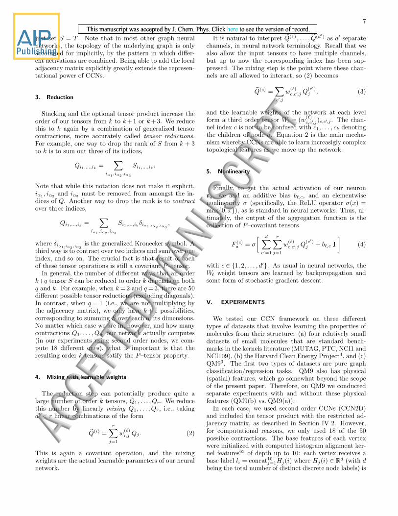
FIG. 4. Feature tensors in a first order CCN for ethylene (C2H4) assuming three channels (red, green, and blue). Verticese1, e2, e5, e6 are hydrogen atoms, while vertices e3, e4 are carbons. Edge (e3, e4) is a double bond, the other edges are singlebonds. (a) At the input layer, the receptive field for each atom is just the atom itself, so the feature matrix has size 1× 3. (b)At level `= 1 the size of the receptive field of each atom grows depending on the local topology. The receptive fields for eachhydrogen atoms grows to include its neighboring carbon atom, resulting in a feature tensor of size 2× 3; the receptive fields ofthe carbon atoms grow to include four atoms each, and therefore have size 4× 3. (c) At layer `= 2, the receptive fields of thecarbons will include every atom in the molecule, while the receptive fields of the hydrogens will only be of size 4.

of representation should not be confused with the neuralnetworks sense of representations of objects, as in “fi isa representation of Pi”).

The representation theory of symmetric groups is arich subject that goes beyond the scope of the presentpaper61. However, there is one particular representationof Sm that is likely familiar even to non-algebraists, theso-called defining representation, given by the Pπ ∈Rn×npermutation matrices

[Pπ]i,j =

{1 if π(j) = i

0 otherwise.

It is easy to verify that Pπ2π1 = Pπ2Pπ1 for any π1,π2 ∈Sm, so {Pπ}π∈Sm is indeed a representation of Sm. If thetransformation rules of the fi activations in a given comp-net are dictated by this representation, then each fi mustnecessarily be a |Pi| dimensional vector, and intuitivelyeach component of fi carries information related to onespecific atom in the receptive field, or the interaction ofthat specific atom with all the others collectively. Wecall this case first order permutation covariance.

Definition 3 We say that ni is a first order covariantnode in a comp-net if under the permutation of its re-ceptive field Pi by any π ∈ S|Pi|, its activation transformsas fi 7→ Pπfi.

If (Rg)g∈G is a representation of a group G, the matri-ces (Rg⊗Rg)g∈G also form a representation. Thus, onestep up in the hierarchy from Pπ–covariant comp-netsare Pπ ⊗ Pπ–covariant comp-nets, where the fi featurevectors are now |Pi|2 dimensional vectors that trans-form under permutations of the internal ordering by πas fi 7→ (Pπ ⊗ Pπ)fi. If we reshape fi into a matrixFi ∈R|Pi|×|Pi|, then the action

Fi 7→ PπFiP>π

is equivalent to Pπ⊗Pπ acting on fi. In the following, wewill prefer this more intuitive matrix view, since it makes

it clear that feature vectors that transform this way ex-press relationships between the different constituents ofthe receptive field. Note, in particular, that if we de-fine A↓Pi as the restriction of the adjacency matrix toPi (i.e., if Pi = (ep1 , . . . , epm) then [A↓Pi ]a,b = Apa,pb),then A↓Pi transforms exactly as Fi does in the equationabove.

Definition 4 We say that ni is a second order co-variant node in a comp-net if under the permutationof its receptive field Pi by any π ∈ S|Pi|, its activation

transforms as Fi 7→ PπFiP>π .

Taking the pattern further lets us define third, fourth,and general, k’th order nodes, in which the activationsare k’th order tensors, transforming under permutationsas Fi 7→ F ′i , where

[F ′i ]j1,...,jk = [Pπ]j1,j′1 [Pπ]j2,j′2 . . . [Pπ]jk,j′k [Fi]j′1,...,j′k .

(1)Here and in the following, for brevity, we use the Einsteinsummation convention, whereby any dummy index thatappears twice on the right hand side of an equation isautomatically summed over.

In general, we will call any quantity which trans-forms under permutations according to (1) a k’th or-der P-tensor. Saying that a given quantity is a P–tensor then not only means that it is representable byan m×m× . . .×m array, but also that this array trans-forms in a specific way under permutations.

Since scalars, vectors and matrices can be considered0th, 1st and 2nd order tensors, the following definitioncovers both quasi-invariance and first and second ordercovariance as special cases. To unify notation and termi-nology, in the following we will always talk about featuretensors rather than feature vectors, and denote the acti-vations as Fi rather than fi.

Definition 5 We say that ni is a k’th order covari-ant node in a comp-net if the corresponding activation

6

Fi is a k’th order P–tensor, i.e., it transforms underpermutations of Pi according to (1), or the activation isa sequence of d separate P–tensors F

(1)i , . . . , F

(d)i corre-

sponding to d distinct channels.

A covariant compositional network (CCN) is acomp-net in which each node’s activation is covariantto permutations in the above sense. Hence we can talkabout first, second, third, etc. order CCNs (CCN 1D,2D,. . . ). In the first few layers of the network, however,the order of the nodes might be lower (Figure 4).

The real significance of covariance, both here and inclassical CNNs, is that while it allows for a richer internalrepresentation of the data than fully invariant architec-tures, the final ouput of the network can still easily bemade invariant. In covariant comp-nets this is achievedby collapsing the input tensors of the root node nr atthe top of the network into invariant scalars, for exam-ple by computing their sums and traces (reducing themto zeroth order tensors), and outputting permutation in-variant combinations of these scalars, such as their sum.

IV. COVARIANT AGGREGATION FUNCTIONS

It remains to explain how to define the Φ aggregationfunctions so as to guarantee covariance. Specifically, weshow how to construct Φ such that if the Fc1 , ..., Fck in-puts of a given node na at level ` are covariant k’th orderP–tensors, then Fa = Φ(Fc1 , ..., Fck) will also be a k’thorder P–tensor. The aggregation function that we de-fine consists of five operations executed in sequence: pro-motion, stacking, reduction, mixing, and an elementwisenonlinear transform. Practically relevant CCNs tend tohave multiple channels, so each Fci is actually a sequenceof d separate P–tensors F

(1)ci , . . . , F

(d)ci . However, except

for the mixing step, each channel behaves independently,so for simplicity, for now we drop the channel index.

1. Promotion

Each child tensor Fci captures information about adifferent receptive field Pci , so before combining themwe must “promote” each Fci to a |Pa| × . . .× |Pa| ten-sor Fci , whose dimensions are indexed by the vertices ofPa rather than the vertices in each Pci . Assuming thatPci = (eq1 , . . . , eq|Pci|

) and Pb = (ep1 , . . . , ep|Pp|), this is

done by defining a |Pa|× |Pci | indicator matrix

χci→ai,j =

{1 if qj = pi0 otherwise,

and setting

[Fci ]j1,...,jk =

[χci→b]j1,j′1 [χci→b]j2,j′2 . . . [χci→b]jk,j′k [Fci ]j′1,...,j′k ,

v

F3

F1

F2F0

T =

[Q1]i,j =∑

k Ti,j,k

[Q2]i,j =∑

k Ti,k,j

[Q1]i,j =∑

k Ti,i,j

F (c) = σ(∑

j

wc,jQj + bc1)

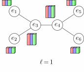
FIG. 5. Schematic of the aggregation process at a given vertexv of G in a second order CCN not involving tensor productswith A↓Pb and assuming a single input channel. Feature ten-sors F0, . . . , F3 are collected from the neighbors of v as wellas from v itself, promoted, and stacked to form a third ordertensor T . In this example we compute just three reductionsQ1, Q2, Q3. These are then combined them with the wc,j

weights and passed through the σ nonlinearity to form theoutput tensors (F (1), F (2), F (3)). For simplicity, in this figurethe “`” and “a” indices are suppressed.

where, once again, Einstein summation is in use, so sum-mation over j′1, . . . , j

′k is implied. Effectively, the promo-

tion step aligns all the child tensors by permuting theindices of Fci to conform to the ordering of the atoms inPa, and padding with zeros where necessary.

2. Stacking

Now that the promoted tensors Fc1 , ..., Fcs all have thesame shape, they can be stacked to form a |Pa|×. . .×|Pa|dimensional k+1’th order tensor T , with

Tj0,...,jk =

[Fci ]j0,...,jk if Pci is the subgraph

centered at epj0 ,

0 otherwise.

It is easy to see that T itself transforms as a P -tensor oforder (k + 1).

We may also add additional information to T by takingits tensor product with another P -tensor. In particular,to explicitly add information about the local topology,we may tensor multiply T by [A↓Pa ]i,j = Aepi ,epj , therestriction of the adjacency matrix to Pa. This will givean order (k + 3) tensor S = T ⊗ A↓Pa . Otherwise, we

7

just set S = T . Note that in most other graph neuralnetworks, the topology of the underlying graph is onlyaccounted for implicitly, by the pattern in which differ-ent activations are combined. Being able to add the localadjacency matrix explicitly greatly extends the represen-tational power of CCNs.

3. Reduction

Stacking and the optional tensor product increase theorder of our tensors from k to k+1 or k+3. We reducethis to k again by a combination of generalized tensorcontractions, more accurately called tensor reductions.For example, one way to drop the rank of S from k + 3to k is to sum out three of its indices,

Qi1,...,ik =∑

iα1,iα2

,iα3

Si1,...,ik .

Note that while this notation does not make it explicit,iα1

, iα2and iα3

must be removed from amongst the in-dices of Q. Another way to drop the rank is to contractover three indices,

Qi1,...,ik =∑

iα1,iα2

,iα3

Si1,...,ikδiα1,iα2,iα3

,

where δiα1,iα2,iα3

is the generalized Kronecker symbol. Athird way is to contract over two indices and sum over oneindex, and so on. The crucial fact is that result of eachof these tensor operations is still a covariant P–tensor.

In general, the number of different ways that an orderk+q tensor S can be reduced to order k depends on bothq and k. For example, when k= 2 and q= 3, there are 50different possible tensor reductions (excluding diagonals).In contrast, when q = 1 (i.e., we are not multiplying bythe adjacency matrix), we only have k+ 1 possibilities,corresponding to summing S over each of its dimensions.No matter which case we are in, however, and how manycontractions Q1, . . . , Qd′ our network actually computes(in our experiments using second order nodes, we com-pute 18 different ones), what is important is that theresulting order k tensors satify the P–tensor property.

4. Mixing with learnable weights

The reduction step can potentially produce quite alarge number of order k tensors, Q1, . . . , Qr. We reducethis number by linearly mixing Q1, . . . , Qr, i.e., takingd′ < r linear combinations of the form

Q(i) =

r∑

j=1

w(`)i,j Qj . (2)

This is again a covariant operation, and the mixingweights are the actual learnable parameters of our neuralnetwork.

It is natural to interpret Q(1), . . . , Q(d′) as d′ separatechannels, in neural network terminology. Recall that wealso allow the input tensors to have multiple channels,but up to now the corresponding index has been sup-pressed. The mixing step is the point where these chan-nels are all allowed to interact, so (2) becomes

Q(c) =∑

c′,j

w(`)c,c′,j Q

(c′)j , (3)

and the learnable weights of the network at each levelform a third order tensor W` = (w

(`)c,c′,j)c,c′,j . The chan-

nel index c is not to be confused with c1, . . . , ck denotingthe children of node a. Equation 2 is the main mecha-nism whereby CCNs are able to learn increasigly complextopological features as we move up the network.

5. Nonlinearity

Finally, to get the actual activation of our neuronna, we add an additive bias b`,c, and an elementwisenonlinearity σ (specifically, the ReLU operator σ(x) =max{0, x}), as is standard in neural networks. Thus, ul-timately, the output of the aggregation function is thecollection of P–covariant tensors

F (c)a = σ

[ d∑

c′=1

r∑

j=1

w(`)c,c′,j Q

(c′)j + b`,c 1

](4)

with c ∈ {1, 2, . . . , d′}. As usual in neural networks, theW` weight tensors are learned by backpropagation andsome form of stochastic gradient descent.

V. EXPERIMENTS

We tested our CCN framework on three differenttypes of datasets that involve learning the properties ofmolecules from their structure: (a) four relatively smalldatasets of small molecules that are standard bench-marks in the kernels literature (MUTAG, PTC, NCI1 andNCI109), (b) the Harvard Clean Energy Project4, and (c)QM93. The first two types of datasets are pure graphclassification/regression tasks. QM9 also has physical(spatial) features, which go somewhat beyond the scopeof the present paper. Therefore, on QM9 we conductedseparate experiments with and without these physicalfeatures (QM9(b) vs. QM9(a)).

In each case, we used second order CCNs (CCN2D)and included the tensor product with the restricted ad-jacency matrix, as described in Section IV 2. However,for computational reasons, we only used 18 of the 50possible contractions. The base features of each vertexwere initialized with computed histogram alignment ker-nel features63 of depth up to 10: each vertex receives abase label li = concat10j=1Hj(i) where Hj(i) ∈ Rd (with dbeing the total number of distinct discrete node labels) is

8

MUTAG PTC NCI1 NCI109

Wesifeiler–Lehman kernel33 84.50 ± 2.16 59.97 ± 1.60 84.76 ± 0.32 85.12 ± 0.29Wesifeiler–Lehman edge kernel33 82.94 ± 2.33 60.18 ± 2.19 84.65 ± 0.25 85.32 ± 0.34Shortest path kernel29 85.50 ± 2.50 59.53 ± 1.71 73.61 ± 0.36 73.23 ± 0.26Graphlets kernel31 82.44 ± 1.29 55.88 ± 0.31 62.40 ± 0.27 62.35 ± 0.28Random walk kernel28 80.33 ± 1.35 59.85 ± 0.95 TIMED OUT TIMED OUTMultiscale Laplacian graph kernel62 87.94 ± 1.61 63.26 ± 1.48 81.75 ± 0.24 81.31 ± 0.22PSCN(k = 10)37 88.95 ± 4.37 62.29 ± 5.68 76.34 ± 1.68 N/ANeural graph fingerprints21 89.00 ± 7.00 57.85 ± 3.36 62.21 ± 4.72 56.11 ± 4.31Second order CCN (our method) 91.64 ± 7.24 70.62 ± 7.04 76.27 ± 4.13 75.54 ± 3.36

TABLE I. Classification results on the kernel datasets (accuracy ± standard deviation).

the vector of relative frequencies of each label for the setof vertices at distance equal to j from vertex i. The net-work was chosen to be three levels deep, with the numberof output channels at each level fixed to 10.

To run our experiments, we used our own custom-builtneural network library called GraphFlow64. Writing ourown deep learning software became necessary because atthe time we started work on the experiments, none of thestandard frameworks such as TensorFlow65, PyTorch66

or MXNet67 had efficient support for the type of tensoroperations required by CCN. GraphFlow is a fast, generalpurpose deep learning library that offers automatic differ-entiation, dynamic computation graphs, multithreading,and GPU support for tensor contractions. In addition toCCN, it also implements other graph neural networks, in-cluding Neural Graph Fingerprints21, PSCN37 and GatedGraph Neural Networks40. We also provide a referenceimplementation of CCN1D and CCN2D in PyTorch68.

In each experiment we used 80% of the dataset fortraining, 10% for validation, and 10% for testing. Forthe kernel datasets we performed the experiments on 10separate training/validation/test stratified splits and av-eraged the resulting classification accuracies. Our train-ing technique used mini-batch stochastic gradient descentwith the Adam optimization method69 and a batch sizeof 64. The initial learning rate was set to 0.001, anddecayed linearly after each step towards a minimum of10−6.

A. Graph kernel datasets

Our first set of experiments involved three standard“graph kernels” datasets: (1) MUTAG, which is a datasetof 188 mutagenic aromatic and heteroaromatic com-pounds,70 (2) PTC, which consists of 344 chemical com-pounds that have been tested for positive or negativetoxicity in lab rats,71 (3) NCI1 and NCI109, which have4110 and 4127 compounds respectively, each screenedfor activity against small cell lung cancer and ovar-ian cancer lines72. In each of these datasets, eachmolecule has a discrete label (i.e., toxic/non-toxic, aro-matic/heteroaromatic) and the goal is to predict thislabel. We compare CCN 2D against the graph ker-

nel results reported in Ref. 62 (C-SVM algorithm withthe Weisfeiler–Lehman kernel33, Weisfeiler–Lehman edgekernel33, Shortest Paths Graph Kernel29, GraphletsKernel31 and the Multiscale Laplacian Graph Kernel62),Neural Graph Fingerprints21 (with up to 3 levels and ahidden size of 10) and the “patchy-SAN” convolutionalalgorithm (PSCN)37. The results are presented in Ta-ble I.

B. Harvard Clean Energy Project

The Harvard Clean Energy Project (HCEP)4 datasetconsists of 2.3 million organic compounds that are can-didates for use in solar cells. The inputs are molecu-lar graphs (derived from their SMILES strings), and theregression target is power conversion efficiency (PCE).The experiments were ran on a random sample of 50,000molecules.

On this dataset we compared CCN to the follow-ing algorithms: Lasso, ridge regression, random forests,Gradient Boosted Trees (GBT), the Optimal Assign-ment Wesifeiler–Lehman Graph Kernel33, Neural GraphFingerprints21, and PSCN37. For the first four of thesebaseline methods, we created simple feature vectors fromeach molecule: the number of bonds of each type (i.e.number of H–H bonds, number of C–O bonds, etc.) andthe number of atoms of each type. Molecular graph fin-gerprints uses atom labels of each vertex as base features.For ridge regression and Lasso, we cross-validated overλ. For random forests and GBT, we used 400 trees, andcross validated over maximum depth, minimum samplesfor a leaf, minimum samples to split a node, and learningrate (for GBT). For Neural Graph Fingerprints, we usedup to 3 layers and a hidden layer size of 10. In PSCN,we used a patch size of 10 with two convolutional layersand a dense layer on top as described in their paper.

C. QM9 Dataset

QM9 has recently emerged as a molecular datasetof significant interest. QM9 contains ∼134k organicmolecules with up to nine atoms (C, H, O, N and F)

9

Test MAE Test RMSE

Lasso 0.867 1.437Ridge regression 0.854 1.376Random forest 1.004 1.799Gradient boosted trees 0.704 1.005Weisfeiler–Lehman kernel33 0.805 1.096Neural graph fingerprints21 0.851 1.177PSCN (k= 10)37 0.718 0.973Second order CCN (our method) 0.340 0.449

TABLE II. HCEP regression results. Error of predictingpower conversion efficiency in units of percent.

out of the GDB-17 universe of molecules. Each moleculeis described by a SMILES string, which is converted tothe molecular graph. The molecular properties are thencalculated using DFT at the level of either B3LYP or 6-31G(2df,p), returning the spatial configurations of eachatom, along with thirteen molecular properties:

(a) U0: atomization energy at 0 Kelvin (eV),(b) U : atomization at room temperature (eV),(c) H: enthalpy of atomization at room temperature

(eV),(d) G: free energy of atomization (eV),(e) ω1: highest fundamental vibrational frequency

(cm−1),(f) ZPVE: zero point vibrational energy (eV),(g) HOMO: highest occupied molecular orbital, energy

of the highest occupied electronic state (eV),(h) LUMO: lowest unoccupied molecular orbital, energy

of the lowest unoccupied electronic state (eV),(i) GAP: difference between HOMO and LUMO (eV),(j) R2: electronic spatial extent (Bohr2),(k) µ: norm of the dipole moment (Debye),(l) α: norm of the static polarizability (Bohr3),(m) Cv: heat capacity at room temp. (cal/mol/K).

We performed two experiments on the QM9 dataset,with the goal of providing a benchmark of CCN as agraph learning framework, and demonstrating that ourframework can predict molecular properties to the samelevel as DFT. In both cases, we trained our system oneach of the thirteen target properties of QM9 indepen-dently, and report the MAE for each.

1. QM9(a)

We use the QM9 dataset to benchmark the CCN ar-chitecture against the Weisfeiler–Lehman graph kernel,Neural Graph Fingerprints, and PSCN. For this test weconsider only heavy atoms and exclude hydrogen. TheCCN architecture is as described above, and settings forNGF and PSCN are as described for HCEP.

WLGK NGF PSCN CCN 2D

α (Bohr3) 3.75 3.51 1.63 1.30Cv (cal/(mol K)) 2.39 1.91 1.09 0.93G (eV) 4.84 4.36 3.13 2.75GAP (eV) 0.92 0.86 0.77 0.69H (eV) 5.45 4.92 3.56 3.14HOMO (eV) 0.38 0.34 0.30 0.23LUMO (eV) 0.89 0.82 0.75 0.67µ (Debye) 1.03 0.94 0.81 0.72ω1 (cm−1) 192.16 168.14 152.13 120.10R2 (Bohr2) 154.25 137.43 61.70 53.28U (eV) 5.41 4.89 3.54 3.02U0 (eV) 5.36 4.85 3.50 2.99ZPVE (eV) 0.51 0.45 0.38 0.35

TABLE III. QM9(a) regression results (mean absolute er-ror). Here we have only used the graph as the learning inputwithout any physical features.

CCN DFT error

α (Bohr3) 0.22 0.4Cv (cal/(mol K)) 0.07 0.34G (eV) 0.06 0.1GAP (eV) 0.12 1.2H (eV) 0.06 0.1HOMO (eV) 0.09 2.0LUMO (eV) 0.09 2.6µ (Debye) 0.48 0.1ω1 (cm−1) 2.81 28R2 (Bohr2) 4.00 -U (eV) 0.06 0.1U0 (eV) 0.05 0.1ZPVE (eV) 0.0039 0.0097

TABLE IV. The mean absolute error of CCN compared toDFT error when using the complete set of physical featuresused in Ref. 25 in addition to the graph of each molecule.

2. QM9(b)

To compare to DFT error, we performed a test ofthe QM9 dataset with each molecule including hydro-gen atoms. We used both physical atomic informa-tion (vertex features) and bond information (edge fea-tures) including: atom type, atomic number, acceptor,donor, aromatic, hybridization, number of hydrogens,Euclidean distance and Coulomb distance between pairsof atoms. All the information is encoded in a vectorizedformat. Our physical features were taken directly fromthe dataset used in Ref. 25 without any special featureengineering.

To include the edge features into our model along withthe vertex features, we used the concept of line graphsfrom graph theory. We constructed the line graph foreach molecular graph in such a way that an edge of themolecular graph corresponds to a vertex in its line graph,and if two edges in the molecular graph share a commonvertex then there is an edge between the two correspond-

10

e1

e2

e3 e4

e5

e6

(1)

(2)

(3)

(4)

(5)

(3)

(4)(1)

(2) (5)

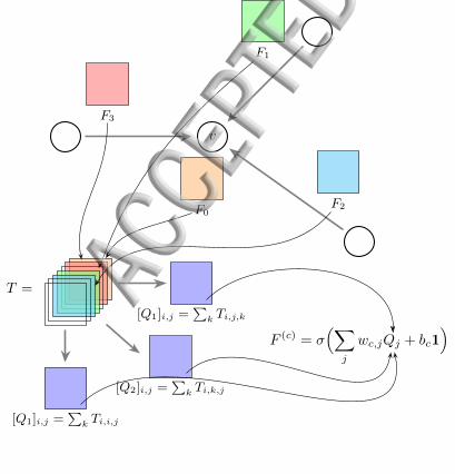
FIG. 6. Molecular graph of C2H4 (left) and its correspondingline graph (right). The vertices of the line graph correspondto edges of the molecular graph; two vertices of the line graphare connected by an edge if their corresponding edges on themolecular graph share a vertex.

ing vertices in the line graph. (See Fig. 6). The edgefeatures become vertex features in the line graph. Theinputs of our model contain both the molecular graphand its line graph. The feature vectors F` between thetwo graphs are merged at each level `.

We present results for both the CCN 1D and CCN 2Darchitectures. For CCN 1D, our network is seven layerswith 64 input channels; at the first and second layer thenumber of channels is halved, and beyond that each layerhas 16 channels. For the CCN 2D architecture, we usedthree layers, with 32 channels at the input and 16 andthe remaining layers. We report the mean average errorfor each learning target in its corresponding physical unitand compare it against the DFT error given in Ref. 25.

D. Discussion

Overall, our CCN outperforms the other algorithms ona significant fraction of the experiments we implemented.On the subsampled HCEP dataset, CCN outperforms allother methods by a very large margin. For the graph ker-nels datasets, the SVM with the Weisfeiler–Lehman ker-nels achieve the highest accuracy on NCI1 and NCI109,while CCN wins on MUTAG and PTC. Perhaps this poorperformance is to be expected, since the datasets aresmall and neural networks usually require tens of thou-sands of training examples to be effective. Indeed, neuralgraph fingerprints and PSCN also perform poorly com-pared to the Weisfeiler–Lehman kernels. In the QM9(a)experiment, CCN obtains better results than the threeother graph learning algorithms on all 13 learning tar-gets.

In the QM9(b) experiment, the error of CCN is smallerthan that of DFT itself on 11 of 12 learning targets(Ref. 25 does not have DFT error for R2). However,other recent works14,25 have obtained even stronger re-sults. Looking at our results, we find that values de-pending strongly on position information, such as thedipole moment and average electronic spatial extent, arepredicted poorly when we include physical features. Incontrast, properties that are not expected to strongly de-pend on spatial extent are predicted significantly better.This suggests that our spatial input features were notfully exploited, and that feature engineering position in-formation could significantly enhance the power of our

CCN.Our custom deep learning library64 enabled all the

above results to be obtained reasonably efficiently. Theprediction time for CCN 1D and CCN 2D on QM9(b)comes out to 6.0 ms/molecule and 7.2 ms/molecule, re-spectively, making it possible to search through a millioncandidate molecules in under two hours.

VI. CONCLUSIONS

In this paper we presented a general framework calledcovariant compositional networks (CCNs) for learningthe properties of molecules from their graphs. Centralto this framework are two key ideas: (1) a compositionalstructure that generalizes message passing neural net-works (MPNNs) and (2) the concept of covariant aggre-gation functions based on tensor algebra.

We argue that CCNs can extract multiscale structurefrom molecular graphs and keep track of the local topol-ogy in a manner the MPNNs are not able to. We alsointroduced the GraphFlow software library that providesan efficient implementation of CCNs. Using GraphFlow,we were able to show that CCNs often outperform ex-isting state-of-the-art algorithms in learning molecularproperties.

ACKNOWLEDGEMENTS

The authors would like to thank the Institute forPure and Applied Mathematics and the participants ofits “Understanding Many Particle Systems with Ma-chine Learning” program for inspiring this research. Ourwork was supported by DARPA Young Faculty AwardD16AP00112, and used computing resources provided bythe University of Chicago Research Computing Center.

1P. Hohenberg and W. Kohn, Phys. Rev. 136, 864 (1964).2Y. LeCun, Y. Bengio, and G. Hinton, Nature 521, 436444(2015).

3R. Ramakrishnan, P. O. Dral, M. Rupp, and O. A. von Lilienfeld,Sci. Data 1 (2014).

4J. Hachmann, R. Olivares-Amaya, S. Atahan-Evrenk,C. Amador-Bedolla, R. S. Sanchez-Carrera, A. Gold-Parker,L. Vogt, A. M. Brockway, and A. Aspuru-Guzik, J. Phys. Chem.Lett. 2, 22412251 (2011).

5S. Kirklin, J. E. Saal, B. Meredig, A. Thompson, J. W. Doak,M. Aykol, S. Ruhl, and C. Wolverton, NPJ Comput. Mat. 1,15010 (2015).

6K. Hansen, F. Biegler, R. Ramakrishnan, W. Pronobis, O. A. vonLilienfeld, K.-R. Muller, and A. Tkatchenko, J. Chem. Phys. 6,2326 (2015).

7B. Huang and O. A. von Lilienfeld, J. Chem. Phys. 145 (2016).8F. A. Faber, L. Hutchison, , B. Huang, J. Gilmer, S. S. Schoen-holz, G. E. Dahl, O. Vinyals, S. Kearnes, P. F. Riley, and O. A.von Lilienfeld, J. Chem. Theory Comput. 13, 52555264 (2017).

9O. A. von Lilienfeld, R. Ramakrishnan, M. Rupp, and A. Knoll,Int. J. Quantum Chem. 115 (2015).

10M. Rupp, A. Tkatchenko, K. R. Muller, and O. A. von Lilienfeld,Phys. Rev. Lett. 108 (2012).

11

11K. Hansen, G. Montavon, F. Biegler, S. Fazli, M. Rupp, M. Schef-fler, O. A. von Lilienfeld, A. Tkatchenko, and K.-R. Muller, J.Chem. Theory Comput. 9, 3404 (2013).

12G. Montavon, M. Rupp, V. Gobre, A. Vazquez-Mayagoitia,K. Hansen, A. Tkatchenko, K.-R. Muller, and O. A. von Lilien-feld, New J. Phys. 15 (2013).

13A. P. Bartok, R. Kondor, and G. Csanyi, Phys. Rev. B 87 (2013).14A. P. Bartok, S. De, C. Poelking, N. Bernstein, J. R. Kermode,

G. Csanyi, and M. Ceriotti, Science Advances 3 (2017).15G. Ferre, J.-B. Maillet, and G. Stoltz, J. Chem. Phys. 143,

104114 (2015).16J. Behler and M. Parrinello, Phys. Rev. Lett. 98, 146401 (2007).17J. Behler, J. Chem. Phys. 134, 074106 (2011).18A. V. Shapeev, Multiscale Model. Simul. 14, 1153 (2016).19M. Hirn, S. Mallat, and N. Poilvert, Multiscale Modeling Sim-

ulation 15, 827 (2017).20J. Bruna, W. Zaremba, A. Szlam, and Y. LeCun, Proc. ICLR,3 (2014).

21D. K. Duvenaud, D. Maclaurin, J. Iparraguirre, R. Bombarell,T. Hirzel, A. Aspuru-Guzik, and R. P. Adams, Adv. NIPS, 28,2224 (2015).

22S. Kearns, K. McCloskey, M. Brendl, V. Pande, and P. Riley, J.Comput. Aided Mol. Des. 30, 595 (2016).

23M. M. Bronstein, J. Bruna, Y. LeCun, A. Szlam, and P. Van-dergheynst, IEEE Signal Process. Mag. 34, 18 (2017).

24K. T. Schutt, K. T., F. Arbabzadah, S. Chmiela, K. R. Muller,and A. Tkatchenko, Nat. Commun. 8, 13890 (2017).

25J. Gilmer, S. S. Schoenholz, P. F. Riley, O. Vinyals, and G. E.Dahl, Proc. ICML, 70 (2017).

26K. Schutt, P.-J. Kindermans, H. E. Sauceda Felix, S. Chmiela,A. Tkatchenko, and K.-R. Muller, Proc. NIPS, (2017).

27R. Kondor, T. S. Hy, H. Pan, S. Trivedi, and B. M. Anderson,Proc. ICLR workshops, (2018).

28T. Gartner, NIPS 2002 workshop on unreal data, (2002).29K. M. Borgwardt and H. P. Kriegel, Proc. IEEE ICDM, 5, 74

(2005).30A. Feragen, N. Kasenburg, J. Peterson, M. de Bruijne, and K. M.

Borgwardt, Adv. NIPS, 26 (2013).31N. Shervashidze, S. V. N. Vishwanathan, T. Petri, K. M., and

K. M. Borgwardt, Proc. AISTATS, 12, 488 (2009).32S. V. N. Vishwanathan, N. N. Schraudolf, R. Kondor, and K. M.

Bogwardt, J. Mach. Learn. Res. 11, 1201 (2010).33N. Shervashidze, P. Schweitzer, E. J. van Leeuwan, K. Mehlhorn,

and K. M. Borgwardt, J. Mach. Learn. Res. 12, 2539 (2011).34M. Neumann, R. Garnett, C. Baukhage, and K. Kersting, Ma-chine Learning, 102 (2016).

35R. Kondor and K. M. Borgwardt, Proc. ICML, 25, 496 (2008).36F. Scarselli, M. Gori, A. C. Tsoi, M. Hagenbuchner, and G. Mon-

fardini, IEEE Trans. on Neural Netw. 20, 61 (2009).37M. Niepert, M. Ahmed, and K. Kutzkov, Proc. ICML, 33, 2014

(2016).38Y. LeCun, Y. Bengio, and P. Haffner, Proc. IEEE , 2278 (1998).39A. Krizhevsky, I. Sutskever, and G. E. Hinton, Adv. NIPS, 25,

1097 (2012).40Y. Li, D. Tarlow, M. Brockschmidt, and R. Zemel, Proc. ICLR,4 (2016).

41P. Battaglia, R. Pascanu, M. Lai, D. J. Rezende, andK. Kavukcuoglu, Adv. NIPS, 29, 4502 (2016).

42T. N. Kipf and M. Welling, Proc. ICLR, 5 (2017).43M. Fischler and R. Elschlager, IEEE Trans. Comput. C-22, 67

(1973).44Y. Ohta, T. Kanade, and T. Sakai, Proc. IJCPR, 4, 752 (1978).45Z. W. Tu, X. R. Chen, A. L. Yuille, and S. C. Zhu, Int. J.

Comput. Vis. 63, 113 (2005).46P. F. Felzenszwalb and D. P. Huttenlocher, Int. J. Comput. Vis.61, 55 (2005).

47S. Zhu and D. Mumford, Found. Trends Comput. Graphics Vis.2, 259 (2006).

48P. F. Felzenszwalb, R. B. Girshick, D. McAllester, and D. Ra-manan, IEEE Trans. Pattern Anal. Mach. Intell. 32, 541 (2010).

49B. Weisfeiler and A. A. Lehman, Nauchno-Technicheskaya Infor-matsia 9 (1968).

50R. C. Read and D. G. Corneil, J. Graph Theory 1, 339 (1977).51J. Y. Cai, M. Furer, and N. Immerman, Combinatorica 12, 389

(1992).52T. Cohen and M. Welling, Proc. ICML, 33, 2990 (2016).53D. E. Worrall, S. Garbin, D. Turmukhambetov, and G. J. Bros-

tow, Proc. IEEE CVPR, (2017).54W. T. Freeman and E. H. Adelson, IEEE Trans. Pattern Anal.

Mach. Intell. 13, 891 (1991).55E. P. Simoncelli, W. T. Freeman, E. H. Adelson, and D. J.

Heeger, IEEE Trans. Inf. Theory. 38, 587 (1992).56P. Perona, IEEE Trans. Pattern Anal. Mach. Intell. 17, 488

(1995).57P. C. Teo and Y. Hel-Or, Pattern Recognit. Lett. 16, 7 (1998).58R. Manduchi, P. Perona, and D. Shy, IEEE Trans. on Signal

Process. 46, 1168 (1998).59T. Cohen and M. Welling, Proc. ICLR, 5 (2017).60J.-P. Serre, Linear Representations of Finite Groups, Graduate

Texts in Mathamatics, Vol. 42 (Springer-Verlag, 1977).61B. E. Sagan, The Symmetric Group, Grad. Texts in Math.

(Springer, 2001).62R. Kondor and H. Pan, Adv. NIPS, 29, 2982 (2016).63N. M. Kriege, P. Giscard, and R. Wilson, Adv. NIPS, 20, 1623

(2016).64T. S. Hy, “GraphFlow: a C++ deep learning framework,” https:

//github.com/HyTruongSon/GraphFlow (2017–).65M. Abadi, A. Agarwal, P. Barham, E. Brevdo, Z. Chen, C. Citro,

G. S. Corrado, A. Davis, J. Dean, M. Devin, S. Ghemawat,I. Goodfellow, A. Harp, G. Irving, M. Isard, Y. Jia, R. Joze-fowicz, L. Kaiser, M. Kudlur, J. Levenberg, D. Mane, R. Monga,S. Moore, D. Murray, C. Olah, M. Schuster, J. Shlens, B. Steiner,I. Sutskever, K. Talwar, P. Tucker, V. Vanhoucke, V. Vasudevan,F. Viegas, O. Vinyals, P. Warden, M. Wattenberg, M. Wicke,Y. Yu, and X. Zheng, “TensorFlow: Large-scale machine learn-ing on heterogeneous systems,” (2015), software available fromtensorflow.org.

66A. Paszke, S. Gross, S. Chintala, G. Chanan, E. Yang, Z. DeVito,Z. Lin, A. Desmaison, L. Antiga, and A. Lerer, Adv. NIPS, 30(2017).

67T. Chen, M. Li, Y. Li, M. Lin, N. Wang, M. Wang, T. Xiao,B. Xu, C. Zhang, and Z. Zhang, NIPS workshop, (2016).

68S. Trivedi, T. S. Hy, and H. Pan, “CCN in PyTorch,” https:

//github.com/horacepan/CCN (2017–).69D. P. Kingma and J. Ba, in Proc. ICLR (San Diego, 2015).70A. K. Debnat, R. L. L. de Compadre, G. Debnath, A. J. Shus-

terman, and C. Hansch, J. Med. Chem. 34, 786 (1991).71H. Toivonen, A. Srinivasan, R. D. King, S. Kramer, and

C. Helma, Bioinformatics 19, 1183 (2003).72N. Wale, I. A. Watson, and G. Karypis, Knowl. Info. Sys. 14,

347 (2008).

http://dx.doi.org/10.1063/1.5024797

http://dx.doi.org/10.1063/1.5024797

http://dx.doi.org/10.1063/1.5024797

http://dx.doi.org/10.1063/1.5024797

f1

n1

f2

n2

f3

n3

f4

n4

f5

n5

f6

n6

f7

n7

f8n8

f9n9

f10

n10

fr nr

http://dx.doi.org/10.1063/1.5024797

http://dx.doi.org/10.1063/1.5024797

1

32

4 5 65′

1

32

4 5 6

e1

e2

e3 e4

e5

e6

`=0

e1

e2

e3 e4

e5

e6

`=1

e1

e2

e3 e4

e5

e6

`=2

v

F3

F1

F2F0

T =

[Q1]i,j =∑

k Ti,j,k

[Q2]i,j =∑

k Ti,k,j

[Q1]i,j =∑

k Ti,i,j

F (c) = σ(∑

j

wc,jQj + bc1)

e1

e2

e3 e4

e5

e6

(1)

(2)

(3)

(4)

(5)

(3)

(4)(1)

(2) (5)