predicting mutual fund performance - oxford-man institute · predicting mutual fund performance...
TRANSCRIPT

Predicting Mutual Fund PerformanceOxford, July-August 2013
Allan Timmermann1
1UC San Diego, CEPR, CREATES
Timmermann (UCSD) Predicting fund performance July 29 - August 2, 2013 1 / 51

1 Basic Performance regressions
2 Power in Statistical Tests
3 Bootstrapped measures of fund performance (Kosowski, Timmermann,Wermers, and White, JF 2006)
4 Conditional Models (Ferson-Schadt, JF 1996)
5 Tracking and predicting time-varying skills (Hansen, Lunde, Timmermann andWermers, 2013)
Timmermann (UCSD) Predicting fund performance July 29 - August 2, 2013 2 / 51
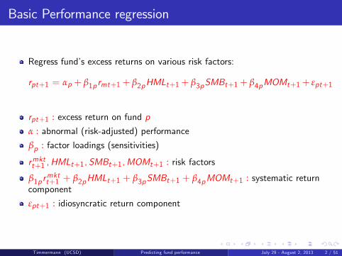
Basic Performance regression
Regress fund’s excess returns on various risk factors:
rpt+1 = αp + β1p rmt+1+ β2pHMLt+1+ β3pSMBt+1+ β4pMOMt+1+ εpt+1
rpt+1 : excess return on fund pα : abnormal (risk-adjusted) performanceβp : factor loadings (sensitivities)
rmktt+1 ,HMLt+1, SMBt+1,MOMt+1 : risk factors
β1p rmktt+1 + β2pHMLt+1 + β3pSMBt+1 + β4pMOMt+1 : systematic return
component
εpt+1 : idiosyncratic return component
Timmermann (UCSD) Predicting fund performance July 29 - August 2, 2013 2 / 51
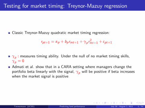
Testing for market timing: Treynor-Mazuy regression
Classic Treynor-Mazuy quadratic market timing regression:
rpt+1 = αp + bp rmt+1 + γp r2mt+1 + εpt+1
γp : measures timing ability. Under the null of no market timing skills,γp = 0
Admati et al. show that in a CARA setting where managers change theportfolio beta linearly with the signal, γp will be positive if beta increaseswhen the market signal is positive
Timmermann (UCSD) Predicting fund performance July 29 - August 2, 2013 3 / 51
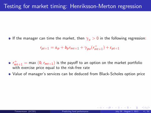
Testing for market timing: Henriksson-Merton regression
If the manager can time the market, then γu > 0 in the following regression:
rpt+1 = αp + bp rmt+1 + γpu(r+mt+1) + εpt+1
r+mt+1 = max (0, rmt+1) is the payoff to an option on the market portfoliowith exercise price equal to the risk-free rate
Value of manager’s services can be deduced from Black-Scholes option price
Timmermann (UCSD) Predicting fund performance July 29 - August 2, 2013 4 / 51
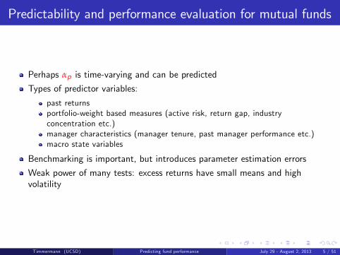
Predictability and performance evaluation for mutual funds
Perhaps αp is time-varying and can be predicted
Types of predictor variables:
past returnsportfolio-weight based measures (active risk, return gap, industryconcentration etc.)manager characteristics (manager tenure, past manager performance etc.)macro state variables
Benchmarking is important, but introduces parameter estimation errors
Weak power of many tests: excess returns have small means and highvolatility
Timmermann (UCSD) Predicting fund performance July 29 - August 2, 2013 5 / 51
Power in performance tests
Power of performance evaluation tests tends to be weak
Economic reasoning suggests that superior performance should not bepervasive across the universe of fund managers
Statistical reasoning suggests that the substantial noise in long-lived assetreturns makes it diffi cult to reliably measure performance in the best ofcircumstances
Timmermann (UCSD) Predicting fund performance July 29 - August 2, 2013 6 / 51

Power in performance tests
Suppose excess returns on a particular mutual fund are generated by theequation
rt = α+ βrmt + εt , εt ∼ N(0, σ2)
rt is the excess return on the fund, β is its beta, rmt is the excess return onthe market portfolio, and εt is the residual in period t
Suppose that α = −0.1%, β = 1, σ = 0.4%. For monthly returns data theseparameter values correspond to a fund that underperforms the index by 1.2percent per year with an annualized idiosyncratic volatility around 1.5%
How many months of data are needed to get a 10/25/50 per cent chance ofcorrectly identifying the fund as an underperformer at the 5% significancelevel (c = 0.05) using a two-sided test?
Timmermann (UCSD) Predicting fund performance July 29 - August 2, 2013 7 / 51

Power in performance tests
Reject the null hypothesis if
∣∣∣∣x − µ0σ/√n
∣∣∣∣ > z1−c/2, i .e., if
x < µ0 − z1−c/2σ/√n, or
x > µ0 + z1−c/2σ/√n
Suppose x ∼ N(µ1, σ/√n). Then
P(x < µ0 − z1−c/2σ/√n) = P(
x − µ1σ/√n<
µ0 − µ1 − z1−c/2σ/√n
σ/√n
)
= P(Z <µ0 − µ1σ/√n− z1−c/2)
= Φ(µ0 − µ1σ/√n− z1−c/2)
Z ∼ N(0, 1) and Φ(.) is the cumulative density function for ZTimmermann (UCSD) Predicting fund performance July 29 - August 2, 2013 8 / 51

Power in performance tests
Likewise
P(x > µ0 + z1−c/2σ/√n) = P(Z >
µ0 − µ1σ/√n+ z1−c/2)
= Φ(µ1 − µ0σ/√n− z1−c/2)
If µ0 = 0, µ1 = −0.1, σ = 0.4, the statistical power becomes
P(reject|µ1, µ0, σ, n) = Power(µ1, µ0, σ, n) = Φ(µ0 − µ1σ/√n− z1−c/2)
+Φ(µ1 − µ0σ/√n− z1−c/2)
= P(Z < −2+ .25√n) + P(Z < −2− .25
√n)
Timmermann (UCSD) Predicting fund performance July 29 - August 2, 2013 9 / 51

Power in performance tests
Using the above parameters, we get
Power required sample size25% 27 (2.25 years)50% 62 (5 years)90% 168 (14 years)
Fund return data is so noisy that it can take very long to detect abnormalperformance with much statistical precision
Performance measurement and evaluation needs to use other data (i.e.portfolio weights) in addition to returns data
Timmermann (UCSD) Predicting fund performance July 29 - August 2, 2013 10 / 51
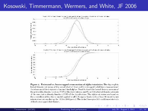
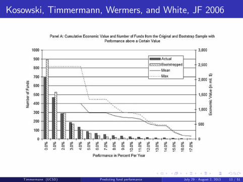
Kosowski, Timmermann, Wermers, and White, JF 2006
Proposes a new bootstrap technique to examine the performance of the U.S.domestic equity mutual fund industry
Bootstrap approach is necessary because the cross section of mutual fundalphas has a complex nonnormal distribution due to heterogeneous risk-takingby funds as well as nonnormalities in individual fund alpha distributions.
Evidence that a sizable minority of managers pick stocks well enough to morethan cover their costs
The superior alphas of these managers persist through time
Timmermann (UCSD) Predicting fund performance July 29 - August 2, 2013 11 / 51
Kosowski, Timmermann, Wermers, and White, JF 2006
Timmermann (UCSD) Predicting fund performance July 29 - August 2, 2013 12 / 51
Kosowski, Timmermann, Wermers, and White, JF 2006
Timmermann (UCSD) Predicting fund performance July 29 - August 2, 2013 13 / 51

Kosowski, Timmermann, Wermers, and White, JF 2006
Timmermann (UCSD) Predicting fund performance July 29 - August 2, 2013 14 / 51
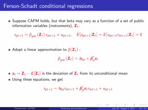
Ferson-Schadt conditional regressions
Suppose CAPM holds, but that beta may vary as a function of a set of publicinformation variables (instruments), Zt :
rpt+1 = βpm (Zt ) rmt+1 + upt+1, E [upt+1 |Zt ] = E [upt+1rmt+1 |Zt ] = 0
Adopt a linear approximation to β(Zt ) :
βpm (Zt ) = b0p + β′pzt
zt = Zt − E [Zt ] is the deviation of Zt from its unconditional mean
Using these equations, we get
rpt+1 = b0p rmt+1 + β′pzt rmt+1 + upt+1
Timmermann (UCSD) Predicting fund performance July 29 - August 2, 2013 15 / 51
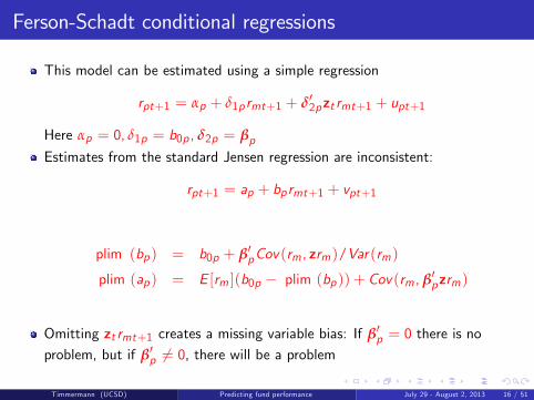
Ferson-Schadt conditional regressions
This model can be estimated using a simple regression
rpt+1 = αp + δ1p rmt+1 + δ′2pzt rmt+1 + upt+1
Here αp = 0, δ1p = b0p , δ2p = βpEstimates from the standard Jensen regression are inconsistent:
rpt+1 = ap + bp rmt+1 + vpt+1
plim (bp) = b0p + β′pCov(rm , zrm)/Var(rm)
plim (ap) = E [rm ](b0p − plim (bp)) + Cov(rm , β′pzrm)
Omitting zt rmt+1 creates a missing variable bias: If β′p = 0 there is noproblem, but if β′p 6= 0, there will be a problem
Timmermann (UCSD) Predicting fund performance July 29 - August 2, 2013 16 / 51
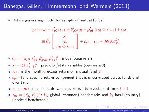
Banegas, Gillen, Timmermann, and Wermers (2013)
Return generating model for sample of mutual funds:
rpt =αp0 + α′p1zt−1 + β′p0rBt + β′p1 (rBt ⊗ zt−1) + εpt
≡ θ′p
xtrBt
rBt ⊗ zt−1
+ εpt , εpt ∼ N(0, σ2p)
θp = (αp0 α′p1 β′p0B β′p1)′ : model parameters
xt = (1 z ′t−1)′ : predictor/state variables (de-meaned)
rpt : is the month-t excess return on mutual fund pεpt : fund-specific return component that is uncorrelated across funds andover time
zt−1 : m demeaned state variables known to investors at time t − 1rBt = (r ′Gt r
′Lt )′ : kG global (common) benchmarks and kL local (country)
unpriced benchmarks
Timmermann (UCSD) Predicting fund performance July 29 - August 2, 2013 17 / 51
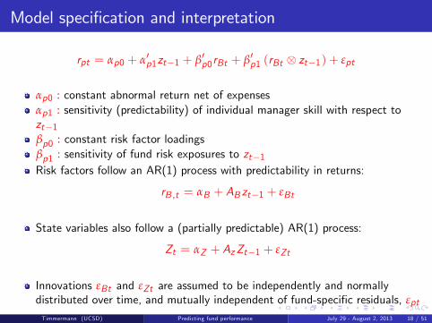
Model specification and interpretation
rpt = αp0 + α′p1zt−1 + β′p0rBt + β′p1 (rBt ⊗ zt−1) + εpt
αp0 : constant abnormal return net of expensesαp1 : sensitivity (predictability) of individual manager skill with respect tozt−1βp0 : constant risk factor loadingsβp1 : sensitivity of fund risk exposures to zt−1Risk factors follow an AR(1) process with predictability in returns:
rB ,t = αB + AB zt−1 + εBt
State variables also follow a (partially predictable) AR(1) process:
Zt = αZ + AzZt−1 + εZt
Innovations εBt and εZt are assumed to be independently and normallydistributed over time, and mutually independent of fund-specific residuals, εpt
Timmermann (UCSD) Predicting fund performance July 29 - August 2, 2013 18 / 51

Restrictions and Beliefs from asset pricing models
Bayesian framework provides a flexible approach to modeling the portfolioimplications of asset pricing models either through dogmatic restrictions onparameter values or prior beliefs on those parameter valuesm state variables and k benchmarks ⇒ 1+m+ k + km location parametersRepresent d dogmatic restrictions on these parameters through thed × (1+m+ k + km) matrix FRPriors follow the standard Normal-Gamma model:
FR θp |σ2p ∼ N(0, σ2p0(d×d )
); σ−2p ∼ G
(s−1, t
)Diffuse beliefs about idiosyncratic variance: s is a constant with degrees offreedom, t, approaching zeroExpress l informative priors through the l × (1+m+ k + km) matrix, FI :
FI θp |σ2p ∼ N(f I ,p , σ
2pΩI
); σ−2p ∼ G
(s−2, t
)ΩI : reflects the tightness of the prior beliefsStandard deviation of prior beliefs on manager skill, αp0 + α′p1zt−1, isdenoted σα
Timmermann (UCSD) Predicting fund performance July 29 - August 2, 2013 19 / 51

Restrictions and Beliefs from asset pricing models
Augment the linear combinations of parameters for which we have dogmaticrestrictions or informative priors with additional uninformative priors overindependent linear combinations of parameters to span the parameter spaceEffectively, we construct a set of uninformative priors, FU , so that thecomplete set of priors is represented by a(1+m+ k + km)× (1+m+ k + km) matrix, F , and the parameters f , Ω:
F =
FRFIFU
; fi =
0(d×1)f I ,p
0(1+m+k+km−d−l )
F θp |σ2p ∼ N
f i , σ2p 0(d×d ) 0 0
0 ΩI 00 0 cI(1+m+k+km−d−l )
≡ N (f p , σ2pΩ)
Express the priors in the form
θp |σ2p ∼ N(F−1f p , σ
2pF−1ΩF ′−1
), σ−2p ∼ G
(s−2, t
)Timmermann (UCSD) Predicting fund performance July 29 - August 2, 2013 20 / 51
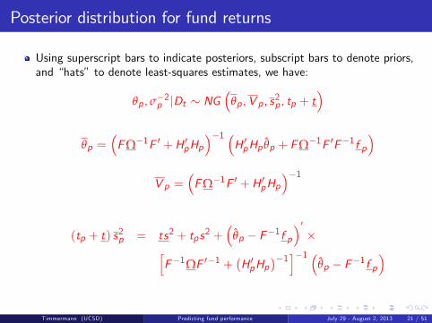
Posterior distribution for fund returns
Using superscript bars to indicate posteriors, subscript bars to denote priors,and “hats” to denote least-squares estimates, we have:
θp , σ−2p |Dt ∼ NG
(θp ,V p , s2p , tp + t
)
θp =(FΩ−1F ′ +H ′pHp
)−1 (H ′pHp θp + FΩ−1F ′F−1f p
)V p =
(FΩ−1F ′ +H ′pHp
)−1
(tp + t) s2p = ts2 + tps2 +(
θp − F−1f p)′×[
F−1ΩF ′−1 +(H ′pHp
)−1]−1 (θp − F−1f p
)
Timmermann (UCSD) Predicting fund performance July 29 - August 2, 2013 21 / 51
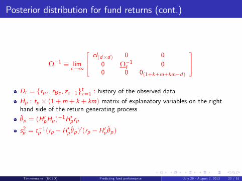
Posterior distribution for fund returns (cont.)
Ω−1 ≡ limc→∞
cI(d×d ) 0 00 Ω−1I 00 0 0(1+k+m+km−d )
Dt = rpτ, rBτ, zτ−1tτ=1 : history of the observed dataHp : tp × (1+m+ k + km) matrix of explanatory variables on the righthand side of the return generating process
θp = (H ′pHp)−1H ′p rp
s2p = t−1p (rp −H ′p θp)′(rp −H ′p θp)
Timmermann (UCSD) Predicting fund performance July 29 - August 2, 2013 22 / 51

Predictive moments for portfolio selection
E [rt |Dt−1 ] = α0 + α1zt−1 + β0A′F xt−1 + β1 (IK ⊗ zt−1) A′F xt−1
≡ α0 + α1zt−1 + βt−1A′F xt−1
V [rt |Dt−1 ] = (1+ δt−1) βt−1ΣB β′t−1 +Ψt−1
Denoting the time-series average of the macro-variables in Dt−1 by z , theremaining variables are defined as:
δt−1 =1
t − 11+ (zt−1 − z) V−1z (zt−1 − z)
Vz =
1t − 1
t−1∑
τ=1(zτ−1 − z) (zτ−1 − z)′
ΣB =1
τB
t−1∑
τ=1εBτ ε′Bτ; εBτ = rBτ − αB − AB zτ−1
Timmermann (UCSD) Predicting fund performance July 29 - August 2, 2013 23 / 51
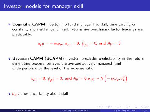
Investor models for manager skill
Dogmatic CAPM investor: no fund manager has skill, time-varying orconstant, and neither benchmark returns nor benchmark factor loadings arepredictable.
αp0 = − expp , αp1 = 0, βp1 = 0, and AB = 0
Bayesian CAPM (BCAPM) investor: precludes predictability in the returngenerating process, believes the average actively managed fundunderperforms by the level of the expense ratio
αp1 = 0, βp1 = 0, and AB = 0, αp0 ∼ N(− expp , σ2α
)
σα : prior uncertainty about skill
Timmermann (UCSD) Predicting fund performance July 29 - August 2, 2013 24 / 51
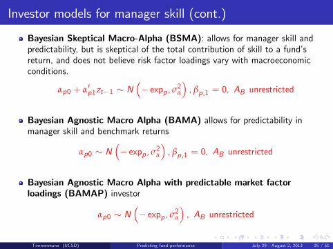
Investor models for manager skill (cont.)
Bayesian Skeptical Macro-Alpha (BSMA): allows for manager skill andpredictability, but is skeptical of the total contribution of skill to a fund’sreturn, and does not believe risk factor loadings vary with macroeconomicconditions.
αp0 + α′p1zt−1 ∼ N(− expp , σ2α
), βp,1 = 0, AB unrestricted
Bayesian Agnostic Macro Alpha (BAMA) allows for predictability inmanager skill and benchmark returns
αp0 ∼ N(− expp , σ2α
), βp,1 = 0, AB unrestricted
Bayesian Agnostic Macro Alpha with predictable market factorloadings (BAMAP) investor
αp0 ∼ N(− expp , σ2α
), AB unrestricted
Timmermann (UCSD) Predicting fund performance July 29 - August 2, 2013 25 / 51
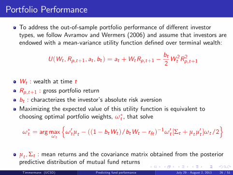
Portfolio Performance
To address the out-of-sample portfolio performance of different investortypes, we follow Avramov and Wermers (2006) and assume that investors areendowed with a mean-variance utility function defined over terminal wealth:
U(Wt ,Rp,t+1, at , bt ) = at +WtRp,t+1 −bt2W 2t R
2p,t+1
Wt : wealth at time tRp,t+1 : gross portfolio returnbt : characterizes the investor’s absolute risk aversionMaximizing the expected value of this utility function is equivalent tochoosing optimal portfolio weights, ω∗t , that solve
ω∗t = argmaxωt
ω′tµt − ((1− btWt )/btWt − rft )−1ω′t [Σt + µtµ
′t ]ωt/2
µt ,Σt : mean returns and the covariance matrix obtained from the posteriorpredictive distribution of mutual fund returns
Timmermann (UCSD) Predicting fund performance July 29 - August 2, 2013 26 / 51
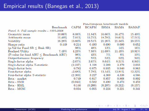
Empirical results (Banegas et al., 2013)
Timmermann (UCSD) Predicting fund performance July 29 - August 2, 2013 27 / 51

Portfolio, country and sector rotation
Timmermann (UCSD) Predicting fund performance July 29 - August 2, 2013 28 / 51
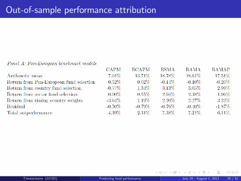
Out-of-sample performance attribution
Timmermann (UCSD) Predicting fund performance July 29 - August 2, 2013 29 / 51
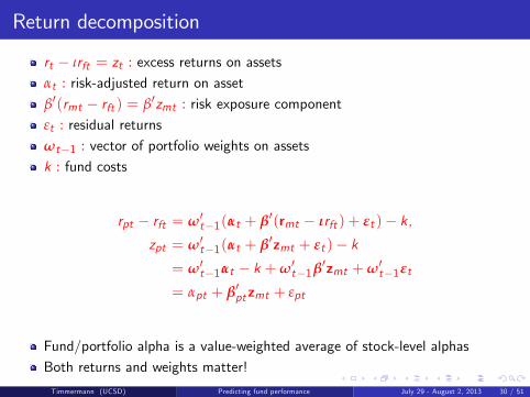
Return decomposition
rt − ιrft = zt : excess returns on assetsαt : risk-adjusted return on assetβ′(rmt − rft ) = β′zmt : risk exposure componentεt : residual returnsωt−1 : vector of portfolio weights on assetsk : fund costs
rpt − rft = ω′t−1(αt + β′(rmt − ιrft ) + εt )− k,zpt = ω′t−1(αt + β′zmt + εt )− k
= ω′t−1αt − k +ω′t−1β′zmt +ω′t−1εt
= αpt + β′ptzmt + εpt
Fund/portfolio alpha is a value-weighted average of stock-level alphasBoth returns and weights matter!
Timmermann (UCSD) Predicting fund performance July 29 - August 2, 2013 30 / 51
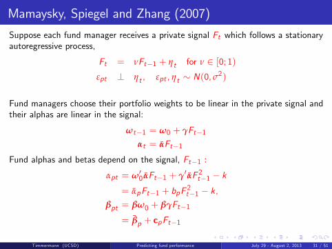
Mamaysky, Spiegel and Zhang (2007)
Suppose each fund manager receives a private signal Ft which follows a stationaryautoregressive process,
Ft = νFt−1 + ηt for ν ∈ [0; 1)εpt ⊥ ηt , εpt , ηt ∼ N(0, σ2)
Fund managers choose their portfolio weights to be linear in the private signal andtheir alphas are linear in the signal:
ωt−1 = ω0 + γFt−1αt = αFt−1
Fund alphas and betas depend on the signal, Ft−1 :
αpt = ω′0 αFt−1 + γ′αF 2t−1 − k= αpFt−1 + bpF
2t−1 − k,
βpt = βω0 + βγFt−1
= βp + cpFt−1
Timmermann (UCSD) Predicting fund performance July 29 - August 2, 2013 31 / 51

The model in state space form
Ft−1 is unobserved, but the model can be put into state space form
zpt = αpFt−1 + bpF2t−1 − k + (β
′p + c
′pFt−1)zmt + εpt
Ft = νFt−1 + ηt
The parameters of this MSZ model can be estimated using the extended KalmanFilter to account for the presence of the squared factor, F 2t−1
Timmermann (UCSD) Predicting fund performance July 29 - August 2, 2013 32 / 51
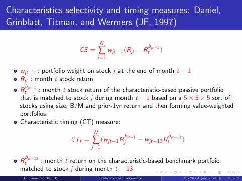
Characteristics selectivity and timing measures: Daniel,Grinblatt, Titman, and Wermers (JF, 1997)
CS =N
∑j=1
wjt−1(Rjt − Rbjt−1t )
wjt−1 : portfolio weight on stock j at the end of month t − 1Rjt : month t stock return
Rbjt−1t : month t stock return of the characteristic-based passive portfoliothat is matched to stock j during month t − 1 based on a 5× 5× 5 sort ofstocks using size, B/M and prior-1yr return and then forming value-weightedportfoliosCharacteristic timing (CT) measure:
CTt =N
∑j=1(wjt−1R
bjt−1j − wjt−13R
bjt−13t )
Rbjt−13t : month t return on the characteristic-based benchmark portfoiomatched to stock j during month t − 13Timmermann (UCSD) Predicting fund performance July 29 - August 2, 2013 33 / 51

MSZ-CS model
Include a second measurement equation in the state space representation whichuses the characteristic selectivity measure CSt in Daniels et al. (1997):
CSt = ω′t−1(zt − zbt ),
zbt : excess returns on characteristic selectivity portfolios chosen to match thecharacteristics of the individual stocks
CSt = ω′t−1(αt + β′zmt + εt −
(αbt + β′bzmt + εbt
))= ω′t−1(αt − αbt ) +ω′t−1(β− βb)
′zmt +ω′t−1(εt − εbt )
= αpt + k −ω′t−1αbt + (βpt − βbt )′zmt + εpt − εbt
= αpFt−1 + bpF2t−1 + εpt − εbt
αbt = 0 because the characteristic-matched stocks are chosen mechanically,βb = β because the exposure to risk factors is matched
Timmermann (UCSD) Predicting fund performance July 29 - August 2, 2013 34 / 51

MSZ-CS and MSZ-CS4 models
Write the state space form of the generalized MSZ-CS and MSZ-CS4 models as(zptCSt
)=
(αpFt−1 + bpF 2t−1 − k
αpFt−1 + bpF 2t−1
)+
(βp + cpFt−1
0
)zmt +
(εpt
εpt − εbt
)Ft = νFt−1 + ηt
Timmermann (UCSD) Predicting fund performance July 29 - August 2, 2013 35 / 51

Conditional models
Ferson and Schadt (1996) time-varying beta
βpm(Xt−1) = ω(Xt−1)′βm(Xt−1)
Xt : l observable information variablesLinearize the beta around E (X) with xt−1 = Xt−1 − E (X).
βpm ≈ bop +B′pxt−1
For appropriately specified b0p and Bp , the fund-level excess return is then
zpt = αpt + b0pzmt +B′pzt−1zmt + εpt
Timmermann (UCSD) Predicting fund performance July 29 - August 2, 2013 36 / 51

Time-varying alpha and beta
Introduce a signal with a linear effect on both the alpha and the portfolio weights:
αt = αFt−1ω(Xt−1) = ω0 + γFt−1 +D′Xt−1
This implies that the fund’s alpha takes the form
αpt = (ω0 + γFt−1 +D′Xt−1)′αFt−1 − k= αpFt−1 + bpF
2t−1 + β′xXt−1Ft−1 − k.
Similarly
b0p =(ω0 + γFt−1 +D′E (X)
)′βm(E (X))
= βp + cpFt−1,
andB′pt−1 = B0p + dpFt−1,
meaning that the beta becomes time-varying
βpm = βp + cpFt−1 +B′pxt−1
Timmermann (UCSD) Predicting fund performance July 29 - August 2, 2013 37 / 51
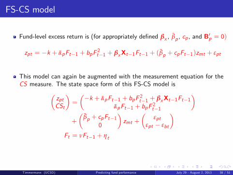
FS-CS model
Fund-level excess return is (for appropriately defined βx , βp , cp , and B′p = 0)
zpt = −k + αpFt−1 + bpF2t−1 + βxXt−1Ft−1 + (βp + cpFt−1)zmt + εpt
This model can again be augmented with the measurement equation for theCS measure. The state space form of this FS-CS model is(
zptCSt
)=
(−k + αpFt−1 + bpF 2t−1 + βxXt−1Ft−1
αpFt−1 + bpF 2t−1
)+
(βp + cpFt−1
0
)zmt +
(εpt
εpt − εbt
)Ft = νFt−1 + ηt
Timmermann (UCSD) Predicting fund performance July 29 - August 2, 2013 38 / 51

Local level models
Local level CS LLcs model uses a state space representation to explore anypersistence in the CS measure:
CS = αpt + εpt = Ft−1 + εpt
Ft = νFt−1 + ηt
This model can be estimated by the standard Kalman Filter, see Durbin andKoopman (2012)
Restricted version, LLcsR imposes ν = 1
Timmermann (UCSD) Predicting fund performance July 29 - August 2, 2013 39 / 51
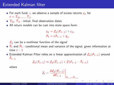
Extended Kalman filter
For each fund, i , we observe a sample of excess returns zit fort = Ti0, . . . ,Ti1Ti0, Ti1 : initial, final observation datesAll return models can be cast into state space form:
zit = Zit (Ft−1) + εit ,
Ft = νFt−1 + ηt ,
Zit can be a nonlinear function of the signalFt and Pt : conditional mean and variance of the signal, given information attime t − 1Extended Kalman Filter relies on a linear approximation of Zit (Ft−1) aroundFt−1
Zit (Ft−1) ≈ Zit (Ft−1) + Z (Ft−1 − Ft−1)where
Zt =∂Zit (Ft−1)
∂Ft−1
∣∣∣∣∣Ft−1=Ft−1
Timmermann (UCSD) Predicting fund performance July 29 - August 2, 2013 40 / 51

Forecast recursions
Given starting values for F0 and P0, the following recursions constitute theextended Kalman Filter:
vt = zit − Zit (Ft−1) Kt = Zt Pt−1Z′t + ε2it
Ft−1|t−1 = Ft−1 + Pt−1Z′tK−1t vt Pt−1|t−1 = Pt−1(I − Z ′tK−1t Zt Pt−1)
Ft = νFt−1|t−1 Pt = ν2Pt−1|t−1 + η2t
ψt : parameter estimates based on time t informationUse Kalman filter to forecast the signal h steps ahead:
Ft+h = Ft+h(ψt ),
αi ,τ+h = αi ,τ+h(Ft−1+h)
Forecast of alpha at time τ + h is a function of the forecast of the signal and theparameter estimates available at time τ.
Timmermann (UCSD) Predicting fund performance July 29 - August 2, 2013 41 / 51
Portfolio Performance
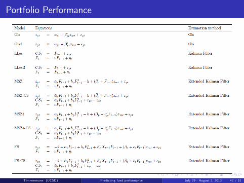
Timmermann (UCSD) Predicting fund performance July 29 - August 2, 2013 42 / 51
Portfolio Performance
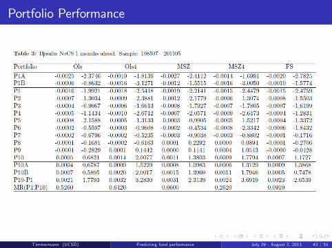
Timmermann (UCSD) Predicting fund performance July 29 - August 2, 2013 43 / 51
Portfolio Performance
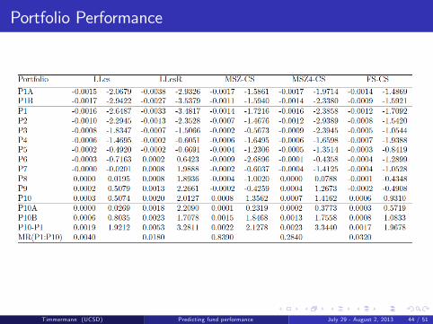
Timmermann (UCSD) Predicting fund performance July 29 - August 2, 2013 44 / 51
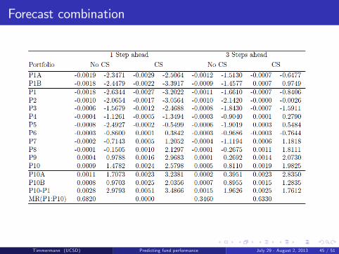
Forecast combination
Timmermann (UCSD) Predicting fund performance July 29 - August 2, 2013 45 / 51
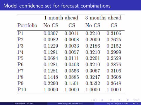
Model confidence set for forecast combinations
Timmermann (UCSD) Predicting fund performance July 29 - August 2, 2013 46 / 51
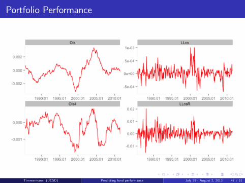
Portfolio Performance
Timmermann (UCSD) Predicting fund performance July 29 - August 2, 2013 47 / 51
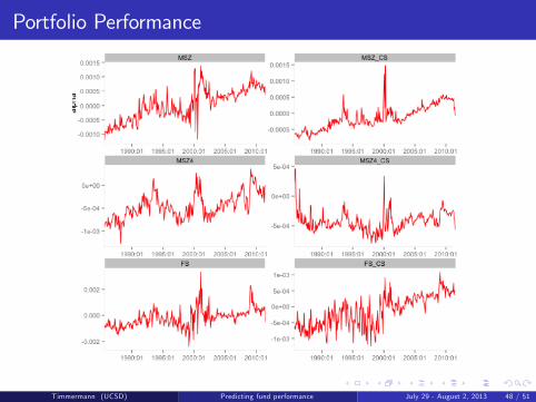
Portfolio Performance
Timmermann (UCSD) Predicting fund performance July 29 - August 2, 2013 48 / 51
Portfolio Performance
Timmermann (UCSD) Predicting fund performance July 29 - August 2, 2013 49 / 51
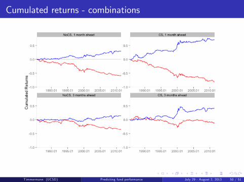
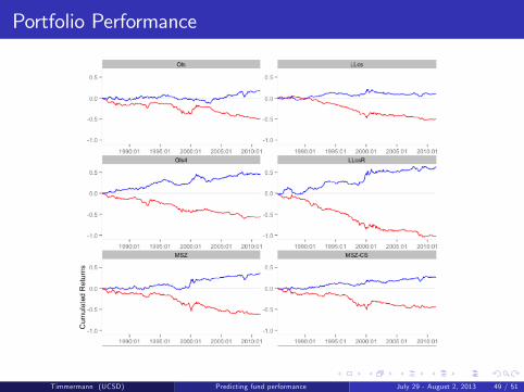
Cumulated returns - combinations
Timmermann (UCSD) Predicting fund performance July 29 - August 2, 2013 50 / 51
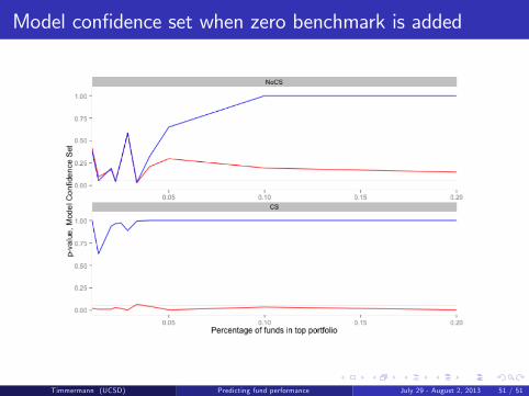
Model confidence set when zero benchmark is added
Timmermann (UCSD) Predicting fund performance July 29 - August 2, 2013 51 / 51